Confronting mass-varying neutrinos with MiniBooNE

Abstract

We study the proposal that mass-varying neutrinos could provide an explanation for the LSND signal for $\bar{\nu}_{\mu}\to\bar{\nu}_{e}$ oscillations. We first point out that all positive oscillation signals occur in matter and that three active mass-varying neutrinos are insufficient to describe all existing neutrino data including LSND. We then examine the possibility that a model with four mass-varying neutrinos (three active and one sterile) can explain the LSND effect and remain consistent with all other neutrino data. We find that such models with a 3 + 1 mass structure in the neutrino sector may explain the LSND data and a null MiniBooNE result for $0.10\mathrel{\raise 1.29167pt\hbox{$<$\kern-7.5pt\lower 4.30554pt\hbox{$\sim$}}}\sin^{2}2\theta_{x}\mathrel{\raise 1.29167pt\hbox{$<$\kern-7.5pt\lower 4.30554pt\hbox{$\sim$}}}0.30$. Predictions of the model include a null result at Double-CHOOZ, but positive signals for underground reactor experiments and for $\nu_{\mu}\to\nu_{e}$ oscillations in long-baseline experiments.

1 Introduction

The LSND experiment has found evidence for $\bar{\nu}_{\mu}\to\bar{\nu}_{e}$ oscillations at the $3.3\sigma$ level [1, 2], with indications for $\nu_{\mu}\to\nu_{e}$ oscillations at lesser significance [2, 3]. The combination of the LSND data with the compelling evidence for oscillations in solar [4, 5, 6, 7], atmospheric [8, 9, 10, 11, 12], accelerator [13], and reactor [14] neutrino experiments cannot be adequately explained in the standard three-neutrino picture [15]. Extensions to models with four light neutrinos (with the extra neutrino being sterile) [16] or $CPT$ violation with three neutrinos [17, 18] have been proposed to accommodate all neutrino data. However, in both cases, recent analyses indicate that neither scenario provides a good description of the complete data set [19, 20]. The addition of a second sterile neutrino improves the fit substantially [22] in some models with more than three neutrinos, especially if there is $CP$ violation [23]. Another possible solution is to have $CPT$ violation in a four-neutrino model [24]. Neutrino decay has also been proposed [25] as a means of explaining the LSND data.

Mass-varying neutrinos [26] (MaVaNs) have been discussed as a means for generating dark energy [27], explaining the LSND results [28] and have been shown to improve the neutrino oscillation fit to solar neutrino data [29]. It is a relevant fact that for all positive oscillation signals (solar, atmospheric, K2K, KamLAND, and LSND) the detected neutrino travels through matter for some or all of its path length. In all but solar neutrino oscillations the path lengths are nearly all through Earth matter, while in the solar case the important matter effects occur in the sun. Therefore if MaVaNs exist, it is possible (although not required) that the masses and mixing angles indicated by the data could differ substantially from their vacuum values.

There are three positive oscillation signals in which the neutrino path is primarily in the Earth’s crust: KamLAND, K2K and LSND. The latest data from K2K [13] now yield an allowed region for the mass-squared difference which is roughly similar to that obtained for the oscillations of atmospheric neutrinos and is inconsistent with the mass scales indicated by KamLAND and LSND neutrino oscillations. The usual argument used to exclude three-neutrino models from solar, atmospheric and LSND data [15] is that there are only two independent mass-squared differences for three neutrinos. This argument applies in the MaVaN scenario to the combination of KamLAND, K2K and LSND experiments, all of which were conducted in Earth matter with similar density (and which therefore should be subject to similar mixings and mass scales). Thus a three-MaVaN model is insufficient to explain all of the data.

In this paper we explore the possibility that oscillations of three active and one sterile MaVaN can explain all neutrino data including LSND and MiniBooNE. Since neutrinos in the KamLAND, K2K and LSND experiments all pass primarily through Earth matter of approximately the same density (Earth crust), they should be consistent with the same set of mixing angles and mass-squared differences. If a set of oscillation parameters cannot be found that is consistent with these three experiments, then a four-MaVaN model is not possible. If such a set can be found, consistency with the solar, atmospheric and vacuum neutrino data must also be realized for the model to be viable. We study only 3 + 1 models, in which there is one mass eigenstate well-separated from the other three, since the constraints on 2 + 2 models are much stronger [19, 30].

For simplicity we examine a minimal 3 + 1 MaVaN scenario in which substantial MaVaN effects occur only for the $\nu_{3}$ and $\nu_{4}$ states and there is no vacuum mixing between active and sterile neutrinos, so that MaVaN effects are solely responsible for active-sterile mixing. We study the feasibility of such a model in describing current data. The MiniBooNE experiment [31] is now taking data that will test the LSND oscillation parameters in the $\nu_{\mu}\to\nu_{e}$ channel; we examine the consequences of this 3 + 1 MaVaN model for both positive and negative MiniBooNE results. We find that viable solutions exist if MiniBooNE sees no oscillations. Furthermore, in those solutions both the vacuum neutrino masses in the active sector and the MaVaN mass terms need not exhibit a hierarchy, and the mass scales for the oscillations of both atmospheric and LSND neutrinos are generated by MaVaN effects. Solar neutrino and KamLAND data are explained primarily by vacuum masses and mixings. Finally, we discuss the implications of this model for future experiments.

2 A 3 + 1 MaVaN model

2.1 Masses and mixings

An element of the mass-squared matrix for MaVaNs in the vacuum eigenstate basis can be written as

$$(M^{2})_{ij}=(m_{i}\delta_{ij}-M_{ij})^{2}\,,$$ (1)

where the $m_{i}$ are the masses in an environment dominated by the cosmic microwave background and the $M_{ij}$ are the density-dependent mass terms generated by acceleron couplings to matter fields. We will assume that the heaviest neutrinos have masses of ${\cal{O}}(0.01)$ eV in the present epoch, and that as a result of their non-negligible velocities, the neutrino overdensity in the Milky Way from gravitational clustering can be neglected [32]. The $m_{i}$ (which we will refer to as vacuum masses) represent the masses of terrestrial neutrinos in laboratory experiments like those measuring tritium beta decay [33]. We note that cosmological bounds on the sum of neutrino masses of ${\cal{O}}(1)$ eV [34] are inapplicable to MaVaNs. Consequently, the usual relationship between neutrino dark matter and neutrinoless double beta decay [35] is also rendered inapplicable. In Ref. [36], it was pointed out that so long as the acceleron does not couple to nonrelativistic neutrino eigenstates (which is the case under consideration), neutrino dark energy is stable. However, the stability of neutrino dark energy with the acceleron also coupled to matter has not been studied so far.

We adopt a matter dependence of the form [29]

$$M_{ij}(n_{e})=M_{ij}^{0}\left(n_{e}\over n_{e}^{0}\right)^{k}\,,$$ (2)

where $n_{e}$ is the electron number density in units of $N_{A}/$cm³, $M_{ij}^{0}$ are the values at some reference density $n_{e}^{0}$ and $k$ parametrizes a power law dependence of the neutrino mass on density. In principle, $M_{ij}$ is expected to depend linearly on $n_{e}$ since the acceleron is assumed to evolve adiabatically and remain at the minimum of its potential. We allow $k$ to deviate from unity to emphasize that a wider range of $k$ is allowed by oscillation data. The choice of reference density is arbitrary; we will take it to be that of the Earth’s crust, $n_{e}^{0}\simeq 1.5$. Implicit in the form of Eq. (2) is the assumption that the neutrino number density has a negligible effect on neutrino masses. Thus, it applies only in the current epoch when the cosmic neutrino background number density (${\cal{O}}(10^{-12})$ eV³) is tiny. At earlier epochs, the neutrino number density is orders of magnitude larger and must be taken into account. For example, in the era of Big Bang Nucleosynthesis, the neutrino number density is ${\cal{O}}(10^{30})$ eV³. Moreover, we have no reason to expect the $M_{ij}^{0}$ to be unaltered at earlier epochs since the acceleron-matter couplings may vary with redshift.

For simplicity we will study a MaVaN model in which MaVaN effects occur only for $\nu_{3}$ and $\nu_{4}$ and there is no vacuum mixing between active and sterile neutrinos. The rationale for this choice is that if MaVaN effects are to be responsible for generating the LSND mass-squared difference and for mixing between active and sterile neutrinos in the Earth, then if they also involve the two lightest neutrinos it would be difficult to obtain the proper mass-squared difference for solar neutrinos. Then the evolution equations in the flavor basis for MaVaN oscillations in matter at the reference density is given by

$$i{d\over dL}\pmatrix{\nu_{e}\cr\nu_{\mu}\cr\nu_{\tau}\cr\nu_{s}}={1\over 2E_{\nu}}\left[UM^{2}U^{\dagger}+A\pmatrix{1&0&0&0\cr 0&0&0&0\cr 0&0&0&0\cr 0&0&0&r}\right]\pmatrix{\nu_{e}\cr\nu_{\mu}\cr\nu_{\tau}\cr\nu_{s}}\,,$$ (3)

where

$$M^{2}=\pmatrix{m_{1}^{2}&0&0&0\cr 0&m_{2}^{2}&0&0\cr 0&0&(m_{3}-M_{33})^{2}&M_{34}^{2}\cr 0&0&M_{34}^{2}&(m_{4}-M_{44})^{2}}\,,$$ (4)

$U$ is the neutrino mixing matrix that connects the flavor eigenstates with the mass eigenstates in vacuum, given by

$$U=\pmatrix{U_{e1}&U_{e2}&U_{e3}&0\cr U_{\mu 1}&U_{\mu 2}&U_{\mu 3}&0\cr U_{\tau 1}&U_{\tau 2}&U_{\tau 3}&0\cr 0&0&0&1}=\pmatrix{c_{x}c_{s}&c_{x}s_{s}&s_{x}&0\cr-c_{a}s_{s}-s_{a}c_{s}s_{x}&c_{a}c_{s}-s_{a}s_{s}s_{x}&c_{x}s_{a}&0\cr s_{a}s_{s}-c_{a}c_{s}s_{x}&-s_{a}c_{s}-c_{a}s_{s}s_{x}&c_{x}c_{a}&0\cr 0&0&0&1}\,,$$ (5)

and $s_{j}$ and $c_{j}$ denote $\sin\theta_{j}$ and $\cos\theta_{j}$, respectively, for $j=s,a,x$. The angle $\theta_{s}$ represents the usual mixing for solar neutrinos, $\theta_{a}$ the mixing for atmospheric neutrinos, and $\theta_{x}$ the mixing of $\nu_{e}$ with $\nu_{\mu}$ in atmospheric and long-baseline experiments. The charged-current amplitude for $\nu_{e}-e$ forward scattering in matter is [37]

$$A=2\sqrt{2}G_{F}n_{e}E_{\nu}=1.52\times 10^{-7}{\rm eV}^{2}\,n_{e}E_{\nu}({\rm MeV})\,.$$ (6)

There is also a $\nu-e$ neutral-current forward scattering contribution for all active neutrinos given by $-Ar$, where $r=n_{n}/(2n_{e})$ and $n_{n}$ is the neutron number density in units of $N_{A}/$cm³, which is equivalent to a $+Ar$ term for the sterile neutrino (see Eq. 3).

It is convenient to parametrize the mass-squared matrix in matter in terms of its eigenvalues $M_{i}^{2}$ and the mixing angle $\theta$ that diagonalizes it,

$$M^{2}=\pmatrix{1&0&0&0\cr 0&1&0&0\cr 0&0&\cos\theta&-\sin\theta\cr 0&0&\sin\theta&\cos\theta}\pmatrix{M_{1}^{2}&0&0&0\cr 0&M_{2}^{2}&0&0\cr 0&0&M_{3}^{2}&0\cr 0&0&0&M_{4}^{2}}\pmatrix{1&0&0&0\cr 0&1&0&0\cr 0&0&\cos\theta&\sin\theta\cr 0&0&-\sin\theta&\cos\theta}\,;$$ (7)

then the mass-squared differences are $\delta M_{ij}^{2}=M_{i}^{2}-M_{j}^{2}$. If the ordinary matter term can be ignored (which will be approximately true for all but solar neutrinos), the neutrino mixing between the mass eigenstates in matter and the flavor eigenstates is

$$V=U\pmatrix{1&0&0&0\cr 0&1&0&0\cr 0&0&\cos\theta&-\sin\theta\cr 0&0&\sin\theta&\cos\theta}=\pmatrix{U_{e1}&U_{e2}&cU_{e3}&-sU_{e3}\cr U_{\mu 1}&U_{\mu 2}&cU_{\mu 3}&-sU_{\mu 3}\cr U_{\tau 1}&U_{\tau 2}&cU_{\tau 3}&-sU_{\tau 3}\cr 0&0&s&c}\,,$$ (8)

where $s\equiv\sin\theta$ and $c\equiv\cos\theta$. For solar neutrinos, where the ordinary matter terms are important, $V$ cannot easily be written in closed form. Since the MaVaN terms do not affect the first and second generations, $M_{1}=m_{1}$ and $M_{2}=m_{2}$.

In 3 + 1 models there is one neutrino mass well-separated from the others by the LSND mass-squared difference ($\delta m^{2}_{L}$), and the sterile neutrino couples strongly only to the isolated state. The atmospheric and solar mass-squared differences will be denoted by $\delta m^{2}_{a}$ and $\delta m^{2}_{s}$, respectively. There are four possible mass spectra in 3 + 1 models, depending on whether the isolated state is above or below the others, and whether the other three neutrino states have a normal ($\delta m^{2}_{a}>0$) or inverted ($\delta m^{2}_{a}<0$) mass hierarchy. We only consider the case with $M_{4}>M_{1},M_{2},M_{3}$ and normal hierarchy, which implies $\delta M^{2}_{43}\simeq\delta M^{2}_{42}\simeq\delta M^{2}_{41}=\delta m^{2}_{L}\gg\delta M^{2}_{32}\simeq\delta M^{2}_{31}=\delta m^{2}_{a}\gg\delta M^{2}_{21}=\delta m^{2}_{s}$.

For now we take $m_{1}=M_{1}=0$, so that $m_{2}^{2}=M_{2}^{2}=\delta m^{2}_{s}$, $M_{3}^{2}=\delta m^{2}_{a}$ and $M_{4}^{2}=\delta m^{2}_{L}$ (we discuss the case $m_{1}\neq 0$ in Sec. 4). We will also set $m_{4}=0$, i.e., the sterile neutrino is massless in vacuum. In our illustration we take $\sin^{2}2\theta_{s}=0.80$ and $\sin^{2}2\theta_{a}=1.00$, and allow $\theta_{x}$ to vary. For the remaining parameters ($m_{3},M_{33},M_{34},M_{44}$) we have the following relations that follow from the diagonalization of $M^{2}$ (Eqs. 4 and 7):

$$(m_{3}-M_{33})^{2}=c^{2}M_{3}^{2}+s^{2}M_{4}^{2}\,,$$ (9)

$$M_{44}^{2}=s^{2}M_{3}^{2}+c^{2}M_{4}^{2}\,,$$ (10)

$$M_{34}^{2}=sc(M_{3}^{2}-M_{4}^{2})\,.$$ (11)

We will also assume that the vacuum masses $m_{2}$ and $m_{3}$ are much smaller than the MaVaN parameters in the Earth’s crust ($M_{33}$, $M_{44}$ and $M_{34}$), which will be justified by our numerical results in Sec. 3.

In order to determine the allowed MaVaN parameters, we will use the positive oscillation results from KamLAND, K2K and LSND. Since these experiments were conducted in the Earth’s crust, the mixing matrix $V$ for all of them should be nearly the same; we will consider it as the same matrix for all three experiments and attempt to determine the parameters from the combined data. Since the baselines for these experiments are all 250 km or less, ordinary matter effects due to coherent forward scattering are small and the $A$ term in Eq. (3) can be ignored to a good approximation. Therefore the mass-squared differences relevant for oscillations in these experiments are $\delta M^{2}_{ij}$ and the mixing matrix is $V$ in Eq. (8).

There are also constraints from other experiments, but only those experiments which were conducted primarily in Earth matter are relevant for the matrix that describes the results of KamLAND, K2K and LSND. The CHOOZ [38] reactor constraint on $\bar{\nu}_{e}\to\bar{\nu}_{e}$ oscillations at the $\delta m^{2}_{a}$ scale ($L/E_{\nu}\simeq 250$ m/MeV) does not apply since the neutrino path in the CHOOZ experiment was primarily in air; it is instead replaced by the weaker Palo Verde [39] constraint at a somewhat smaller $L/E_{\nu}$ value. Similarly, bounds from the Bugey reactor experiment [40] at the $\delta m^{2}_{L}$ scale ($L/E_{\nu}\simeq 25$ m/MeV) must be replaced by the considerably weaker bounds from Gosgen [41] and Krasnoyarsk [42]. The CDHSW [43] bound on $\nu_{\mu}\to\nu_{\mu}$ oscillations at the $\delta m^{2}_{L}$ scale applies to the Earth matter case, as the neutrino path was approximately 90% in matter in this experiment [44]. Once the MaVaN parameters have been determined from the Earth crust data, consistency with the atmospheric, solar and vacuum data can be checked.

2.2 Oscillation formulas

In this section we list the oscillation probabilities in the limit that the ordinary matter effect can be ignored, except for solar neutrino oscillations. The relevant oscillation probabilities in the leading oscillation are approximately

$$P(\bar{\nu}_{\mu}\to\bar{\nu}_{e})_{\rm LSND} \simeq 4s^{4}|U_{\mu 3}|^{2}|U_{e3}|^{2}\sin^{2}\Delta_{L}\,,$$ (12)

$$P(\nu_{\mu}\to\nu_{\mu})_{\rm CDHSW} \simeq 1-4s^{2}|U_{\mu 3}|^{2}(1-s^{2}|U_{\mu 3}|^{2})\sin^{2}\Delta_{L}\,,$$ (13)

$$\bar{P}(\bar{\nu}_{e}\to\bar{\nu}_{e})_{\rm Gosgen} \simeq 1-4s^{2}|U_{e3}|^{2}(1-s^{2}|U_{e3}|^{2})\sin^{2}\Delta_{L}\,,$$ (14)

where $\Delta_{L}$ is the largest of the usual oscillation arguments $\Delta_{j}=\delta m^{2}_{j}L/(4E_{\nu})$ for $j=L$, $s$, $a$.

The relevant oscillation probabilities at the first subleading scale ($\delta m^{2}_{a}$) are approximately

$$P(\nu_{\mu}\to\nu_{\mu})_{\rm K2K} \simeq 1-2s^{2}|U_{\mu 3}|^{2}(1-s^{2}|U_{\mu 3}|^{2})-4c^{2}|U_{\mu 3}|^{2}(1-|U_{\mu 3}|^{2})\sin^{2}\Delta_{a}$$ (15)

$$P(\nu_{\mu}\to\nu_{e})_{\rm K2K} \simeq 2s^{4}|U_{e3}|^{2}|U_{\mu 3}|^{2}+4c^{2}|U_{e3}|^{2}|U_{\mu 3}|^{2}\sin^{2}\Delta_{a}\,,$$ (16)

$$P(\nu_{\mu}\to\nu_{s})_{\rm K2K} \simeq 2s^{2}c^{2}|U_{\mu 3}|^{2}\,,$$ (17)

$$P(\bar{\nu}_{e}\to\bar{\nu}_{e})_{\rm PaloVerde} \simeq \sin^{2}2\theta_{x}\left[{1\over 2}s^{4}+c^{2}\sin^{2}\Delta_{a}\right]\,,$$ (18)

where we have averaged over the leading oscillation scale. We do not consider $CP$ violation, so the oscillation probabilities for neutrinos and anti-neutrinos are the same.

At the smallest scale ($\delta m^{2}_{s}$) we have

$$P(\bar{\nu}_{e}\to\bar{\nu}_{e})_{\rm KamLAND} \simeq 1-2|U_{e3}|^{2}(1-|U_{e3}|^{2})-2s^{2}c^{2}|U_{e3}|^{4}-4|U_{e1}|^{2}|U_{e2}|^{2}\sin^{2}\Delta_{s}\,,$$ (19)

where we have averaged over the oscillations of the two higher $\delta m^{2}$ scales. For solar neutrinos, for the large mixing angle (LMA) solution with adiabatic propagation we have

$$P(\nu_{e}\to\nu_{e})=\sum_{j=1}^{4}|U_{ej}|^{2}|V_{ej}^{0}|^{2}\,,$$ (20)

where $V^{0}$ is the corresponding value of $V$ at the point in the sun where the neutrino is created ($n_{e}\simeq 80$). The fraction of solar neutrinos that oscillate to sterile neutrinos is given by

$$P(\nu_{e}\to\nu_{s})=\sum_{j=1}^{4}|U_{ej}|^{2}|V_{sj}^{0}|^{2}\,.$$ (21)

3 Model constraints

3.1 Fits to Earth crust data

As discussed above, KamLAND, K2K and LSND should all be described with the $\delta M^{2}_{ij}$ and mixing $V$ that exist in the Earth’s crust ($n_{e}\simeq 1.5$). KamLAND data [14] give $\delta m^{2}_{s}\simeq 8\times 10^{-5}$ eV² with oscillation amplitude 0.8 and the K2K results [13] imply $\delta m^{2}_{a}\simeq 2.8\times 10^{-3}$ eV² with maximal mixing (both in two-neutrino fits). In a three-neutrino model, if the mixing angle $\theta_{x}$ vanishes, then these two oscillations decouple from one another [45] and the two-neutrino fits may be used directly. However, the amplitude of the LSND oscillation is (from Eq. 12)

$$\sin^{2}2\theta_{L}=s^{4}s_{a}^{2}\sin^{2}2\theta_{x}\,,$$ (22)

so a non-zero $\theta_{x}$ is required to generate an LSND signal. We will examine solutions with small sterile mixing ($\sin^{2}\theta\ll 1$), so that reactor constraints at the $\delta m^{2}_{a}$ scale are similar to the usual three-neutrino case (see Eq. 18). Similarly, the oscillation probabilities for KamLAND and solar neutrinos are approximately the same as in the three-neutrino case (see Eq. 19 and Section 3.3). There are upper bounds on $\theta_{x}$ from three-neutrino fits [46]: $\sin^{2}2\theta_{x}\leq 0.19~{}(0.28)$ from solar and KamLAND data and $\sin^{2}2\theta_{x}\leq 0.16~{}(0.23)$ from CHOOZ, atmospheric and K2K data, where the bounds are at the $2\sigma$ ($3\sigma$) level. However, for MaVaNs traveling through the Earth’s crust the CHOOZ bound is no longer applicable and must be replaced by the Palo Verde constraint, which is less restrictive by approximately a factor of two at the $\delta m^{2}_{a}$ indicated by K2K and atmospheric neutrinos ($\approx 2-3\times 10^{-3}$ eV²). Therefore, a value of $\sin^{2}2\theta_{x}$ as large as $\simeq 0.3$ would appear to be allowed at the $3\sigma$ level with the CHOOZ constraint removed.

Finally, it is well-known that a combination of reactor and accelerator constraints disfavor the standard 3 + 1 model [19, 47]. In our 3 + 1 MaVaN model, the strong bounds from the Bugey reactor are replaced by the considerably weaker bounds (by approximately a factor of three) from Gosgen and Krasnoyarsk. In the region of interest ($\delta m^{2}_{L}\simeq 1$ eV²) the upper bound on the $\nu_{\mu}\to\nu_{\mu}$ oscillation amplitude from CDHSW is about 0.1; the corresponding bound on the $\bar{\nu}_{e}\to\bar{\nu}_{e}$ oscillation amplitude from Gosgen/Krasnoyarsk is also about 0.1. From Eqs. (13) and (14) we see that in this model the oscillation amplitude for Gosgen/Krasnoyarsk is smaller than that for CDHSW by a factor $|U_{e3}/U_{\mu 3}|^{2}=\tan^{2}\theta_{x}/s_{a}^{2}$ (for small $\theta$), which for $\sin^{2}2\theta_{x}\leq 0.3$ and $\theta_{a}=\pi/4$ is of order 0.15 or less. Therefore if the CDHSW bound is satisfied, then the Gosgen/Krasnoyarsk constraints are automatically satisified, and we need to consider only the effect of the CDHSW bound on the model parameters.

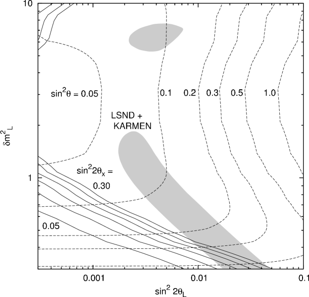
Figure 1: Regions in $\delta m^{2}_{L}$-$\sin^{2}2\theta_{L}$ space accessible to the 3 + 1 MaVaN model discussed in this paper. The solid (dashed) curves show the upper bound on the LSND amplitude $\sin^{2}2\theta_{L}$ from CDHSW for given values of $\sin^{2}2\theta_{x}$ ($\sin^{2}\theta$, the mixing between the third and fourth mass eigenstates due to MaVaN effects). The intersections of the dashed curves with the solid curves show the values of $\sin^{2}\theta$ and $\sin^{2}2\theta_{x}$ required to achieve the maximum LSND amplitudes allowed by CDHSW. The shaded regions show the current 99% C.L. region allowed by a joint analysis [48] of LSND and KARMEN data.

In Fig. 1 we show regions in LSND amplitude $\sin^{2}2\theta_{L}$ and mass-squared difference $\delta m^{2}_{L}$ accessible to the model and the constraints from data. The solid curves are the upper bounds on $\sin^{2}2\theta_{L}$ allowed by the 90% C.L. CDHSW constraint for several values of $\theta_{x}$. The intersections of the dashed curves with the solid curves show the values of $\sin^{2}\theta$ required to achieve those upper bounds; i.e., $s^{4}=2\sin^{2}2\theta_{L}/\sin^{2}2\theta_{x}$ from Eq. (22). The shaded regions show the current 99% C.L. allowed region from a joint analysis [48] of LSND and KARMEN [49] data. For $\sin^{2}2\theta_{x}\leq 0.30$, $\sin^{2}\theta\mathrel{\raise 1.29167pt\hbox{$>$\kern-7.5pt\lower 4.30554pt\hbox{$\sim$}}}0.23$ is required to be consistent with the LSND/KARMEN 99% C.L. allowed region. However, as we will show in the next section, such large values of $\theta$ are not compatible with atmospheric neutrino data.

3.2 Atmospheric neutrinos

Expressions for the oscillation probabilities for atmospheric neutrinos are similar to those for K2K (Eqs. 15-17), except that the values for $\delta M^{2}$ and $V$ vary as the electron number density along the neutrino path varies (there is also an additional matter effect for $\nu_{\mu}\to\nu_{e},\nu_{s}$ oscillations for the higher-energy atmospheric neutrinos, which we ignore). We will call the varying mass and mixing parameters for atmospheric neutrinos $\tilde{M}_{3}^{2}$, $\tilde{M}_{4}^{2}$ and $\tilde{\theta}$. These quantities obey relations similar to Eqs. (9)-(11)

$$(m_{3}-M_{33}r^{k})^{2}=\tilde{c}^{2}\tilde{M}_{3}^{2}+\tilde{s}^{2}\tilde{M}_{4}^{2}\,,$$ (23)

$$M_{44}^{2}r^{2k}=\tilde{s}^{2}\tilde{M}_{3}^{2}+\tilde{c}^{2}\tilde{M}_{4}^{2}\,,$$ (24)

$$M_{34}^{2}r^{2k}=\tilde{s}\tilde{c}(\tilde{M}_{3}^{2}-\tilde{M}_{4}^{2})\,.$$ (25)

with $M_{3}$, $M_{4}$ and $\theta$ replaced by their tilde counterparts and with the MaVaN parameters $M_{33}$, $M_{34}$ and $M_{44}$ multiplied by the factor $r^{k}$, where $r$ is the ratio of the average matter density for a given path compared to the density of the Earth’s crust; e.g., for a path through the center of the Earth, $r\sim 3$. For small $m_{3}$ (the solutions we are investigating) the value of the varying sterile mixing in the Earth, $\tilde{\theta}$, is very similar to the sterile mixing in the crust, $\theta$; this can be seen by comparing the expressions for $\theta$ and $\tilde{\theta}$

$$\tan 2\theta={2M_{34}^{2}\over(m_{3}-M_{33})^{2}-M_{44}^{2}}\qquad,\qquad\tan 2\tilde{\theta}={2M_{34}^{2}r^{2k}\over(m_{3}-M_{33}r^{k})^{2}-M_{44}^{2}r^{2k}}\,.$$ (26)

In the limit that $|m_{3}|\ll|M_{33}|$, it is evident that $\tilde{\theta}\simeq\theta$. Therefore if $\theta$ is small then $\tilde{\theta}$ will also be small, and sterile mixing will not upset the atmospheric neutrino fits. In this same limit the size of $\tilde{M}^{2}_{4}$, i.e., the largest varying oscillation mass scale in the Earth, is approximately $r^{2k}\delta m^{2}_{L}$.

For $\theta_{a}=\pi/4$, the amplitude for oscillation to sterile neutrinos is given approximately by $\tilde{s}^{2}c_{x}^{2}$ (from the tilde equivalent to Eq. 17); these oscillations occur at the leading mass scale ($\mathrel{\raise 1.29167pt\hbox{$>$\kern-7.5pt\lower 4.30554pt\hbox{$\sim$}}}1$ eV²) and oscillations with amplitude of order $\tilde{s}^{2}c_{x}^{2}$ are seen for downward as well as upward neutrinos. Since no large suppression of downward events is observed [10], a value of $\sin^{2}\tilde{\theta}$ (and hence also $\sin^{2}\theta$) greater than about 0.10 is disfavored. As noted in the previous section, if $\sin^{2}2\theta_{x}\leq 0.30$, then the sterile mixing angle must satisfy $\sin^{2}\theta\mathrel{\raise 1.29167pt\hbox{$>$\kern-7.5pt\lower 4.30554pt\hbox{$\sim$}}}0.23$ to obtain a value for the LSND amplitude consistent with the 99% C.L. allowed region from LSND and KARMEN. Therefore, if MiniBooNE (in which the neutrino path is primarily in Earth crust) were to confirm the LSND/KARMEN 99% C.L. allowed region, our 3 + 1 MaVaN model would be disfavored.

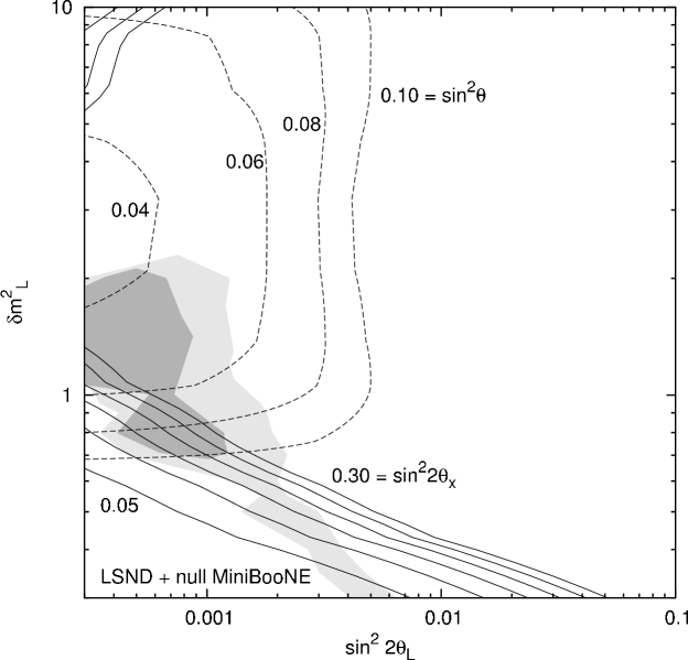
Figure 2: Same as Fig. 1, except that the lighter (darker) shaded region shows the region that would be allowed at 99.5% CL if MiniBooNE sees no signal after running with $5\times 10^{20}$ ($10^{21}$) P.O.T.

The situation changes if MiniBooNE reports a null result. The lighter shaded region in Fig. 2 shows the region that would be allowed (at 99.5% C.L.) by a combination of LSND and a null MiniBooNE result with $5\times 10^{20}$ protons on target (P.O.T.) [50]. This LSND/null-MiniBooNE region is shifted to smaller $\sin^{2}2\theta_{L}$ compared to the LSND/KARMEN region in Fig. 1. This shift occurs because a null MiniBooNE result would be in conflict with LSND, and a combined fit to the two experiments essentially results in a weighted average of the two oscillation probabilities (0.25% from LSND and 0% from MiniBooNE, respectively). Since LSND and MiniBooNE would be in conflict, no region is allowed below the 98% C.L. [50]. As is evident from Fig. 2, this new allowed region could comfortably be explained by our 3 + 1 MaVaN model with both $\sin^{2}2\theta_{x}\mathrel{\raise 1.29167pt\hbox{$<$\kern-7.5pt\lower 4.30554pt\hbox{$\sim$}}}0.30$ and $\sin^{2}\theta\mathrel{\raise 1.29167pt\hbox{$<$\kern-7.5pt\lower 4.30554pt\hbox{$\sim$}}}0.10$, in the region near $\delta m^{2}_{L}\sim 1$ eV² and $\sin^{2}2\theta_{L}\simeq 0.0003-0.001$. An increase to $10^{21}$ P.O.T. in MiniBooNE decreases the size of the combined allowed region but does not eliminate it (see the darker shaded region in Fig. 2); there is no region below the 98.8% C.L. with $10^{21}$ P.O.T. [50]. The smallest value of $\sin^{2}2\theta_{x}$ consistent with the LSND/null-MiniBooNE region is about 0.10 if $\sin^{2}\theta$ is not allowed to be larger than about 0.10, and $\sin^{2}\theta$ must be larger than about 0.04; see Fig. 2.

So far we have considered only the effects of sterile mixing on atmospheric neutrino oscillations, which are more or less independent of the exact neutrino masses in matter, since the effects primarily depend on the size of $\tilde{\theta}$ and not the actual mass-squared differences. However, the mass-varying mass-squared difference that drives the oscillations of atmospheric neutrinos ($\tilde{M}_{3}$) will be different for different neutrino paths through the Earth. We need to show that the model can simultaneously give the correct $\delta m^{2}$ for K2K in the crust and for atmospheric neutrinos.

Although a detailed analysis of atmospheric neutrinos would be required to determine the precise effects of the density profiles on the allowed regions of the parameters, some semi-quantitative statements can be made. Since the largest oscillation signal occurs for upward events, which pass through the core, as a first approximation we consider a path through the center of the Earth as representative of the atmospheric data; the average matter density for these events is $r\simeq 3$ times the density in the Earth’s crust. There are then a total of six potential observables from Eqs. (9)-(11) and (23)-(25): $M_{3}^{2},M_{4}^{2}$ and $\theta$ (from K2K and LSND), and $\tilde{M}_{3}^{2},\tilde{M}_{4}^{2}$ and $\tilde{\theta}$ (from atmospheric neutrinos).

Since the sterile mixing angle $\tilde{\theta}$ for atmospheric neutrinos which pass through the core is very similar to $\theta$ in the crust, its exact value is unimportant, as long as it is small. Furthermore, the value of the largest mass scale for atmospheric neutrinos which pass through the core, $\tilde{M}_{4}^{2}$, is not determined by data since no such oscillations are observed. Therefore the only relevant observable from the upward atmospheric data is the effective mass-squared difference $\tilde{M}_{3}^{2}$; we can rewrite Eqs. (23)-(25) in terms of $\tilde{M}_{3}^{2}$ as

$$M_{34}^{4}r^{4k}+\tilde{M}_{3}^{2}[(m_{3}-M_{33}r^{k})^{2}+M_{44}^{2}r^{2k}]=(m_{3}-M_{33}r^{k})^{2}M_{44}^{2}r^{2k}+\tilde{M}_{3}^{4}\,.$$ (27)

There are four free parameters in Eq. (4): $m_{3}$, $M_{33}$, $M_{34}$ and $M_{44}$. Equations (9)-(11) and (27) can be used to determine these four parameters using the oscillation data as follows: $M_{3}^{2}=\tilde{M}_{3}^{2}=\delta m^{2}_{a}$ (assuming K2K and upward atmospheric neutrinos have the same $\delta m^{2}$) and $M_{4}^{2}=\delta m^{2}_{L}$, where particular values for the vacuum mixing $U$ and sterile mixing angle in the crust $\theta$ are also used as inputs. Once $m_{3},M_{33},M_{44}$ and $M_{34}$ are determined, the size of the LSND amplitude in Eq. (22) can be checked for consistency with the LSND result.

Using $\delta m^{2}_{a}=2.0\times 10^{-3}$ eV² for both K2K and atmospheric neutrinos, Table 1 shows the maximum value of $\sin^{2}\theta$ allowed by CDHSW, the corresponding LSND amplitude $\sin^{2}2\theta_{L}$, and the MaVaN parameters $m_{3},M_{33},M_{34}$ and $M_{44}$ for given values of $\delta m^{2}_{L}$ and $\sin^{2}2\theta_{x}$ with $k=1$ and $r=3$. We see that the $\sin^{2}2\theta_{L}$ values are in the range allowed by the combined LSND/null-MiniBooNE fit (see Fig. 2). The value of $m_{3}$ is small, about 0.006 eV, which confirms our assumption that $|m_{3}|\ll|M_{33}|$. Since the value of $m_{2}$ is $\sqrt{\delta m^{2}_{s}}\simeq 0.009$ eV, then $m_{3}\sim m_{2}$, i.e., all of the non-zero vacuum masses have similar size. Likewise, all the MaVaN parameters $M_{33},M_{34}$ and $M_{44}$ have similar size, of ${\cal O}(1)$ eV. Therefore no hierarchies in either the vacuum masses of the active neutrinos or MaVaN parameters are required to achieve the appropriate masses and mixings.

Table 1: Maximum value of $\sin^{2}\theta$ allowed by CDHSW, the corresponding LSND amplitude $\sin^{2}2\theta_{L}$, and the mass parameters $m_{3},M_{33},M_{34}$ and $M_{44}$, for several sets of values for $\delta m^{2}_{L}$ and $\sin^{2}2\theta_{x}$. The density exponent factor used in Eq. (2) is $k=1$, and the ratio of core path density to crust path density used in Eq. (27) is $r=3$.

$\delta m^{2}_{L}$	$\sin^{2}2\theta_{x}$	$(\sin^{2}\theta)_{max}$	$\sin^{2}2\theta_{L}$	$m_{3}$	$M_{33}$	$M_{34}$	$M_{44}$
(eV2)				(eV)	(eV)	(eV)	(eV)
1.0	0.30	0.063	5.9$\times 10^{-4}$	0.0056	$-$0.249	0.492	0.968
1.0	0.20	0.061	3.7$\times 10^{-4}$	0.0057	$-$0.245	0.489	0.969
0.9	0.30	0.074	8.2$\times 10^{-4}$	0.0055	$-$0.256	0.485	0.913
0.9	0.15	0.071	3.8$\times 10^{-4}$	0.0056	$-$0.251	0.480	0.914
0.8	0.30	0.085	1.1$\times 10^{-3}$	0.0056	$-$0.259	0.472	0.856
0.8	0.15	0.081	4.9$\times 10^{-4}$	0.0057	$-$0.252	0.467	0.858
0.7	0.20	0.100	1.0$\times 10^{-3}$	0.0056	$-$0.262	0.458	0.794
0.7	0.10	0.098	4.8$\times 10^{-4}$	0.0056	$-$0.260	0.456	0.795

Figure 3: Variation of $\tilde{M}_{3}^{2}$ (which determines the $\delta m^{2}$ for atmospheric and long-baseline neutrinos) with electron number density for the first example listed in Table 1. Similar behavior is exhibited for the other examples.

We note that there is some fine tuning required so that the K2K and atmospheric neutrino mass-squared differences are small compared to the LSND scale. This amounts to requiring $|m_{3}-M_{33}|M_{44}\simeq M_{34}^{2}$; since $|m_{3}|\ll|M_{33}|$, this is approximately equivalent to requiring $|M_{33}M_{44}|\simeq M_{34}^{2}$. Since the MaVaN parameters scale similarly with density, this fine tuning is not greatly upset by changes in density, e.g., from the Earth’s crust to its core. This is confirmed by Fig. 3, which shows the value of $\tilde{M}_{3}^{2}$ for the first example in Table 1 as $r$ is increased from 1 to 3. Since $\tilde{M}_{3}^{2}$ and $\tilde{\theta}$ do not vary greatly over the entire range of Earth densities, the oscillation formulas in Sec. 2.2 should provide a good approximation to the actual oscillation probabilities. Furthermore, the model should provide good fits to the atmospheric neutrino data over all zenith angles in which the neutrino path is mostly in the Earth. The parameters $M_{33},M_{34}$ and $M_{44}$ are also changed very little by changes to the input values for $k$ (the power that determines the density dependence of the MaVaN parameters); $m_{3}$ increases by about 10% if $k$ is decreased to $1/2$. Therefore the general features of the model are insensitive to the exact density dependence of the MaVaN effects, to changes in the matter density as the neutrinos traverse the Earth, or to the precise value of the core/crust density ratio.

The pathlength in Earth matter for atmospheric neutrinos is given by

$$L_{m}=\sqrt{R^{2}\cos^{2}\Theta+\sin^{2}\Theta(2R\epsilon-\epsilon^{2})}-(R-\epsilon)\cos\Theta\,,$$ (28)

where $\Theta$ is the zenith angle (zero for downward events), $R$ is the Earth’s radius and $\epsilon$ is the detector depth (of order 1 km). For comparison, the total path length is

$$L=\sqrt{R^{2}\cos^{2}\Theta+\sin^{2}\Theta(2R\epsilon-\epsilon^{2})+2R\delta+\delta^{2}}-(R-\epsilon)\cos\Theta\,,$$ (29)

where $\delta$ is the height above the Earth’s surface at which the neutrino is created (of order 20 km). If $L_{m}$ is a few oscillation lengths or more, the oscillations average and the distinction between $L_{m}$ and $L$ is inconsequential. However, when $L_{m}$ is significantly different from $L$ and the oscillations do not average, the matter mixing angles no longer accurately describe the oscillations. For example, for horizontal events ($\Theta=\pi/2$) the total distance is less than an oscillation length for the atmospheric $\delta m^{2}$ and $L_{m}/L\simeq\sqrt{\epsilon/(\delta+\epsilon)}\simeq\sqrt{1/20}\simeq 0.22$. For events with $\Theta$ near $\pi/2$, the difference between $L_{m}$ and $L$ changes rapidly with $\Theta$; a detailed analysis of atmospheric data is required to determine the precise constraints on the MaVaN parameters.

If $\theta_{a}\neq\pi/4$, i.e., the atmospheric neutrino mixing is not maximal, then the maximum LSND amplitude for a given value of $\theta_{x}$ can be larger, as given by the formula

$$\sin^{2}2\theta_{L}^{max}={(\sin^{2}2\theta_{L}^{max})_{\theta_{a}=\pi/4}\over 1-\cos 2\theta_{a}}.$$ (30)

For example, for $\sin^{2}2\theta_{a}=0.9$ the maximum LSND amplitude increases by about 50%. This has the effect of shifting the solid curves to the right in Figs. 1 and 2 by the same factor. Current data still excludes the model, and the allowed parameters shift somewhat in the scenario where MiniBooNE sees a null result, but the general features remain the same.

3.3 Solar neutrinos

The matter density in the sun is much higher than in the Earth, but since in our model MaVaN effects only occur for $\nu_{3}$ and $\nu_{4}$, $\delta M^{2}_{21}$ has approximately the same value as in the standard MSW scenario for all densities. The effects of sterile mixing are also small since $\nu_{s}$ couples only indirectly to the two lightest states. We have checked numerically that the MSW probability in Eq. (20) including all MaVaN and sterile mixing effects gives the usual result to within about a percent or less for the same values of $\theta_{s}$, $\theta_{a}$ and $\theta_{x}$. Also, we found that the fraction of solar neutrinos that oscillate to steriles (Eq. 21) is less than 1%, which is easily within the range allowed by current data [51]. Therefore the MaVaN mass terms and sterile neutrino mixing have a negligible effect on solar neutrino oscillations in our model.

A non-zero $\theta_{x}$ improves the fit to the intermediate-energy solar neutrinos (compared to the two-neutrino case), at the expense of a slightly worse fit to the low and high-energy solar neutrinos [52]. As noted previously, a value for $\sin^{2}2\theta_{x}$ as large as $\simeq 0.30$ is consistent with combined fits to solar and KamLAND data [46] and does not appear to be ruled out. The range $0.10\mathrel{\raise 1.29167pt\hbox{$<$\kern-7.5pt\lower 4.30554pt\hbox{$\sim$}}}\sin^{2}2\theta_{x}\mathrel{\raise 1.29167pt\hbox{$<$\kern-7.5pt\lower 4.30554pt\hbox{$\sim$}}}0.30$ that would be consistent with LSND and a null MiniBooNE result is also consistent with the solar data.

3.4 Vacuum constraints

The constraints which apply to the experiments primarily in vacuum (Bugey and CHOOZ) must also be checked for consistency with the model. Since the vacuum $m_{3}^{2}$ is of order $\delta m^{2}_{s}$ and the vacuum $m_{4}^{2}=0$, all of the oscillations in vacuum occur with $\delta m^{2}$ values of order $\delta m^{2}_{s}$, not accessible in short baseline experiments. Therefore both the Bugey and CHOOZ bounds are avoided in this model.

We note that there are solutions to Eqs. (9)-(11) and (27) with $m_{4}=0$ other than those listed in Table 1. They have the same sign for $m_{3}$ and $M_{33}$, with $m_{3}\sim M_{ij}$, i.e., all parameters involving $\nu_{3}$ and $\nu_{4}$ are of ${\cal O}(1)$ eV. In that case, there are vacuum oscillations at short baseline due to $m_{3}^{2}\sim 1$ eV². However, such solutions would have $\bar{\nu}_{e}\to\bar{\nu}_{e}$ oscillations at short baseline with approximate amplitude $\sin^{2}2\theta_{x}$ which are ruled out by the Bugey reactor experiment.

4 Discussion

We conclude by discussing some of the main features of our MaVaN model with three active neutrinos and one sterile neutrino designed to explain the LSND data and a null MiniBooNE result:

• The sterile mixing angle in the Earth’s crust ($\theta$) is approximately the same as the sterile mixing angle in the Earth’s core ($\tilde{\theta}$); these angles must obey $\sin^{2}\theta\simeq\sin^{2}\tilde{\theta}\mathrel{\raise 1.29167pt\hbox{$<$\kern-7.5pt\lower 4.30554pt\hbox{$\sim$}}}0.10$ to agree with atmospheric neutrino oscillation data.

• A large part of the region in $\delta m^{2}_{L}$-$\sin^{2}2\theta_{L}$ space consistent with the LSND/null-MiniBooNE region, can be reproduced in this MaVaN model with $0.10\mathrel{\raise 1.29167pt\hbox{$<$\kern-7.5pt\lower 4.30554pt\hbox{$\sim$}}}\sin^{2}2\theta_{x}\mathrel{\raise 1.29167pt\hbox{$<$\kern-7.5pt\lower 4.30554pt\hbox{$\sim$}}}0.30$ and $0.04\mathrel{\raise 1.29167pt\hbox{$<$\kern-7.5pt\lower 4.30554pt\hbox{$\sim$}}}\sin^{2}\theta\mathrel{\raise 1.29167pt\hbox{$<$\kern-7.5pt\lower 4.30554pt\hbox{$\sim$}}}0.10$. The significant size of $\theta_{x}$ means that it should be detectable in proposed reactor experiments with expected sensitivity $\sin^{2}2\theta_{x}\geq 0.01$ where most of the neutrino path is in Earth matter, such as Angra, Braidwood, Daya Bay [53], or KASKA [54]. However, Double-CHOOZ [55], which should be sensitive to $\sin^{2}2\theta_{x}\geq 0.03$, would see a null result since most of the neutrino path is in air (where the $\delta m^{2}$ values are all of order $\delta m^{2}_{s}$). The planned long-baseline experiments MINOS [56] and ICARUS [57], sensitive to $\sin^{2}2\theta_{x}\geq 0.05$ at the 90% C.L.[58], should also see a positive signal in the $\nu_{\mu}\to\nu_{e}$ appearance channel. The large value for $\theta_{x}$ might also be detectable in future measurements of solar neutrinos [52].

• The generic features of the model are relatively insensitive to the precise density dependence of the MaVaN parameters. There is a certain amount of fine tuning between vacuum and MaVaN parameters required to achieve the relation $\delta m^{2}_{a}\ll\delta m^{2}_{L}$ in the Earth, but the mass-squared differences for atmospheric neutrinos are fairly stable under variations in the Earth density.

• The vacuum neutrino masses of the active states are given by $m_{1}=0$, $m_{2}=\sqrt{\delta m^{2}_{s}}\simeq 0.009$ eV and $m_{3}\simeq 0.006$ eV. If we allow $m_{1}=M_{1}$ to be non-zero, it can be of order $m_{2}$ and $m_{3}$ if there is a small upward shift in the eigenvalues $M_{3}^{2}$, $M_{4}^{2}$ and $\tilde{M}_{3}^{2}$ by the non-zero value of $m_{1}^{2}$. This shift does not make an appreciable difference to the parameters in Table 1. In this case there would be neither a hierarchy nor a zero value required in either the vacuum masses of the active neutrinos or in the MaVaN couplings.

• The values of $\delta m^{2}_{a}$ measured in the K2K and atmospheric neutrino experiments do not have to be the same, since they are separate inputs in determining the model parameters. The central value in K2K is about 40% higher than for atmospheric neutrinos (with 90% C.L. uncertainties of order 50%). Although currently not significant, if the discrepancy between $\delta m^{2}$ values for K2K and atmospheric neutrinos persists, it could easily be accommodated in this model.

• It has been shown that MaVaN terms that involve only $\nu_{1}$ and $\nu_{2}$ can improve the fit to solar neutrino data [29]. Diagonal and off-diagonal MaVaN couplings must be introduced for $\nu_{1}$ and $\nu_{2}$; if there are no MaVaN terms coupling $\nu_{1}$ or $\nu_{2}$ with $\nu_{3}$ or $\nu_{4}$, then the phenomenology at the $\delta m^{2}_{a}$ and $\delta m^{2}_{L}$ scales discussed in this paper is unaffected. The MaVaN couplings involving $\nu_{1}$ and $\nu_{2}$ would need to be about three orders of magnitude smaller than those for $\nu_{3}$ and $\nu_{4}$.

• We have chosen to consider only MaVaN couplings that involve the third and fourth generations, so that they do not impact the solar neutrino $\delta m^{2}$ scale for Earth matter densities. Introducing MaVaN terms that couple $\nu_{1}$ or $\nu_{2}$ to $\nu_{3}$ or $\nu_{4}$ can also induce $\nu_{\mu}\to\nu_{e}$ oscillations at the LSND scale, but then at solar densities this mixing upsets the value of the solar $\delta m^{2}$. Although we have not performed an exhaustive parameter search, MaVaN terms that lead to the appropriate LSND amplitude and that also couple appreciably to $\nu_{1}$ and $\nu_{2}$ at Earth matter densities appear to be problematic.

• The MINOS experiment has recently found evidence for $\nu_{\mu}\to\nu_{\mu}$ oscillations at a baseline of 735 km [59] with a $\delta m^{2}$ that is consistent with K2K and atmospheric data. Since the neutrino path in the MINOS experiment traverses matter of similar density as that in the K2K experiment, our model also explains MINOS data.

In summary, we have presented a MaVaN model that can explain all neutrino oscillation results, including LSND, and a null result for $\nu_{\mu}\to\nu_{e}$ oscillations in MiniBooNE. There is no hierarchy required in the vacuum masses of the active neutrinos, which are of ${\cal O}(10^{-2})$ eV, and the density-dependent MaVaN parameters are all of ${\cal O}(1)$ eV for the matter density of the Earth’s crust. Active-sterile mixing is small and is generated solely by MaVaN effects. Due to the large value required for $\theta_{x}$, the model predicts visible oscillation effects in underground reactor neutrino experiments such as Daya Bay and Braidwood, but a null result in the mostly above ground Double-CHOOZ experiment. Long-baseline experiments such as MINOS and ICARUS should see sizeable $\nu_{\mu}\to\nu_{e}$ oscillations.

References

- [1] C. Athanassopoulos et al. [LSND Collaboration], Phys. Rev. C 54, 2685 (1996) [arXiv:nucl-ex/9605001]; Phys. Rev. Lett. 77, 3082 (1996) [arXiv:nucl-ex/9605003].
- [2] A. Aguilar et al., Phys. Rev. D 64, 112007 (2001) [arXiv:hep-ex/0104049].
- [3] C. Athanassopoulos et al. [LSND Collaboration], Phys. Rev. C 58, 2489 (1998) [arXiv:nucl-ex/9706006]; Phys. Rev. Lett. 81, 1774 (1998) [arXiv:nucl-ex/9709006].
- [4] B. T. Cleveland et al., Astrophys. J. 496, 505 (1998).
- [5] J. Hosaka et al. [Super-Kamiokande Collaboration], arXiv:hep-ex/0508053.
- [6] J. N. Abdurashitov et al. [SAGE Collaboration], J. Exp. Theor. Phys. 95, 181 (2002) [Zh. Eksp. Teor. Fiz. 122, 211 (2002)] [arXiv:astro-ph/0204245]; W. Hampel et al. [GALLEX Collaboration], Phys. Lett. B 447, 127 (1999); M. Altmann et al. [GNO Collaboration], Phys. Lett. B 490, 16 (2000) [arXiv:hep-ex/0006034].
- [7] B. Aharmim et al. [SNO Collaboration], arXiv:nucl-ex/0502021.
- [8] K. S. Hirata et al. [KAMIOKANDE-II Collaboration], Phys. Lett. B 205, 416 (1988); Phys. Lett. B 280, 146 (1992).
- [9] D. Casper et al., Phys. Rev. Lett. 66, 2561 (1991); R. Becker-Szendy et al., Phys. Rev. Lett. 69, 1010 (1992).
- [10] Y. Ashie et al. [Super-Kamiokande Collaboration], Phys. Rev. D 71, 112005 (2005) [arXiv:hep-ex/0501064].
- [11] W. W. Allison et al. [Soudan-2 Collaboration], Phys. Lett. B 391, 491 (1997) [arXiv:hep-ex/9611007]; Phys. Lett. B 449, 137 (1999) [arXiv:hep-ex/9901024].
- [12] M. Ambrosio et al. [MACRO Collaboration], Phys. Lett. B 434, 451 (1998) [arXiv:hep-ex/9807005]; Phys. Lett. B 478, 5 (2000) [arXiv:hep-ex/0001044]; Phys. Lett. B 517, 59 (2001) [arXiv:hep-ex/0106049]; arXiv:hep-ex/0304037.
- [13] E. Aliu et al. [K2K Collaboration], Phys. Rev. Lett. 94, 081802 (2005) [arXiv:hep-ex/0411038].
- [14] T. Araki et al. [KamLAND Collaboration], Phys. Rev. Lett. 94, 081801 (2005) [arXiv:hep-ex/0406035].
- [15] O. Yasuda and H. Minakata, arXiv:hep-ph/9602386; C. Y. Cardall and G. M. Fuller, Phys. Rev. D 53, 4421 (1996) [arXiv:astro-ph/9602104].
- [16] D. O. Caldwell and R. N. Mohapatra, Phys. Rev. D 48, 3259 (1993); J. T. Peltoniemi and J. W. Valle, Nucl. Phys. B 406, 409 (1993) [arXiv:hep-ph/9302316]; J. J. Gomez-Cadenas and M. C. Gonzalez-Garcia, Z. Phys. C 71, 443 (1996) [arXiv:hep-ph/9504246]; E. Ma and P. Roy, Phys. Rev. D 52, 4780 (1995) [arXiv:hep-ph/9504342]; E. J. Chun, A. S. Joshipura and A. Y. Smirnov, Phys. Lett. B 357, 608 (1995) [arXiv:hep-ph/9505275]; Phys. Rev. D 54, 4654 (1996) [arXiv:hep-ph/9507371]; R. Foot and R. R. Volkas, Phys. Rev. D 52, 6595 (1995) [arXiv:hep-ph/9505359]; Z. G. Berezhiani and R. N. Mohapatra, Phys. Rev. D 52, 6607 (1995) [arXiv:hep-ph/9505385]; N. Okada and O. Yasuda, Int. J. Mod. Phys. A 12, 3669 (1997) [arXiv:hep-ph/9606411]; S. M. Bilenky, C. Giunti and W. Grimus, Eur. Phys. J. C 1, 247 (1998) [arXiv:hep-ph/9607372]; K. Benakli and A. Y. Smirnov, Phys. Rev. Lett. 79, 4314 (1997) [arXiv:hep-ph/9703465]; V. D. Barger, T. J. Weiler and K. Whisnant, Phys. Lett. B 427, 97 (1998) [arXiv:hep-ph/9712495]; S. C. Gibbons, R. N. Mohapatra, S. Nandi and A. Raychaudhuri, Phys. Lett. B 430, 296 (1998) [arXiv:hep-ph/9803299]; N. Gaur, A. Ghosal, E. Ma and P. Roy, Phys. Rev. D 58, 071301 (1998) [arXiv:hep-ph/9806272]; V. D. Barger, S. Pakvasa, T. J. Weiler and K. Whisnant, Phys. Rev. D 58, 093016 (1998) [arXiv:hep-ph/9806328]; S. M. Bilenky, C. Giunti, W. Grimus and T. Schwetz, Phys. Rev. D 60, 073007 (1999) [arXiv:hep-ph/9903454]; V. D. Barger, B. Kayser, J. Learned, T. J. Weiler and K. Whisnant, Phys. Lett. B 489, 345 (2000) [arXiv:hep-ph/0008019].
- [17] H. Murayama and T. Yanagida, Phys. Lett. B 520, 263 (2001) [arXiv:hep-ph/0010178]; G. Barenboim, L. Borissov, J. Lykken and A. Y. Smirnov, JHEP 0210, 001 (2002) [arXiv:hep-ph/0108199]; G. Barenboim, L. Borissov and J. Lykken, Phys. Lett. B 534, 106 (2002) [arXiv:hep-ph/0201080]; G. Barenboim, J. F. Beacom, L. Borissov and B. Kayser, Phys. Lett. B 537, 227 (2002) [arXiv:hep-ph/0203261].
- [18] G. Barenboim, L. Borissov and J. Lykken, arXiv:hep-ph/0212116.
- [19] M. Maltoni, T. Schwetz, M. A. Tortola and J. W. Valle, arXiv:hep-ph/0405172.
- [20] A. Strumia, Phys. Lett. B 539, 91 (2002) [arXiv:hep-ph/0201134]; M. C. Gonzalez-Garcia, M. Maltoni and T. Schwetz, arXiv:hep-ph/0306226.
- [21] H. Pas, L. G. Song and T. J. Weiler, Phys. Rev. D 67, 073019 (2003) [arXiv:hep-ph/0209373]; see also O. Yasuda, arXiv:hep-ph/0006319.
- [22] M. Sorel, J. Conrad and M. Shaevitz, arXiv:hep-ph/0305255.
- [23] V. Barger, J. Conrad, M. Sorel and K. Whisnant, in preparation.
- [24] V. Barger, D. Marfatia and K. Whisnant, Phys. Lett. B 576, 303 (2003) [arXiv:hep-ph/0308299].
- [25] S. Palomares-Ruiz, S. Pascoli and T. Schwetz, arXiv:hep-ph/0505216.
- [26] M. Kawasaki, H. Murayama and T. Yanagida, Mod. Phys. Lett. A 7, 563 (1992); G. J. Stephenson Jr., T. Goldman and B. H. J. McKellar, Int. J. Mod. Phys. A 13, 2765 (1998) [arXiv:hep-ph/9603392]; Mod. Phys. Lett. A 12, 2391 (1997) [arXiv:hep-ph/9610317]; R. Horvat, Phys. Rev. D 58, 125020 (1998) [arXiv:hep-ph/9802377]; R. F. Sawyer, Phys. Lett. B 448, 174 (1999) [arXiv:hep-ph/9809348]; R. Horvat, JHEP 0208, 031 (2002) [arXiv:hep-ph/0007168]; X. J. Bi, P. h. Gu, X. l. Wang and X. m. Zhang, Phys. Rev. D 69, 113007 (2004) [arXiv:hep-ph/0311022]; P. Q. Hung and H. Pas, Mod. Phys. Lett. A 20, 1209 (2005) [arXiv:astro-ph/0311131]; R. D. Peccei, Phys. Rev. D 71, 023527 (2005) [arXiv:hep-ph/0411137]; E. I. Guendelman and A. B. Kaganovich, arXiv:hep-th/0411188; H. Li, Z. g. Dai and X. m. Zhang, Phys. Rev. D 71, 113003 (2005) [arXiv:hep-ph/0411228]; M. Cirelli, M. C. Gonzalez-Garcia and C. Pena-Garay, Nucl. Phys. B 719, 219 (2005) [arXiv:hep-ph/0503028]; P. h. Gu, X. J. Bi, Z. H. Lin and X. m. Zhang, arXiv:hep-ph/0503120; A. W. Brookfield, C. van de Bruck, D. F. Mota and D. Tocchini-Valentini, arXiv:astro-ph/0503349; R. Horvat, arXiv:astro-ph/0505507; R. Takahashi and M. Tanimoto, arXiv:hep-ph/0507142; R. Fardon, A. E. Nelson and N. Weiner, arXiv:hep-ph/0507235; H. Li, B. Feng, J.-Q. Xia and X. m. Zhang, arXiv:astro-ph/0509272.
- [27] P. Q. Hung, arXiv:hep-ph/0010126; P. Gu, X. Wang and X. Zhang, Phys. Rev. D 68, 087301 (2003) [arXiv:hep-ph/0307148]; R. Fardon, A. E. Nelson and N. Weiner, arXiv:astro-ph/0309800.
- [28] D. B. Kaplan, A. E. Nelson and N. Weiner, Phys. Rev. Lett. 93, 091801 (2004) [arXiv:hep-ph/0401099]; K. M. Zurek, JHEP 0410, 058 (2004) [arXiv:hep-ph/0405141].
- [29] V. Barger, P. Huber and D. Marfatia, Phys. Rev. Lett. 95, 211802 (2005) [arXiv:hep-ph/0502196].
- [30] For a review of models with more than three neutrinos, see V. Barger, D. Marfatia and K. Whisnant, Int. J. Mod. Phys. E 12, 569 (2003) [arXiv:hep-ph/0308123].
- [31] I. Stancu et al. [MiniBooNE collaboration], FERMILAB-TM-2207
- [32] S. Singh and C. P. Ma, Phys. Rev. D 67, 023506 (2003) [arXiv:astro-ph/0208419]; A. Ringwald and Y. Y. Y. Wong, JCAP 0412, 005 (2004) [arXiv:hep-ph/0408241].
- [33] C. Weinheimer, arXiv:hep-ex/0210050; V. M. Lobashev et al., Nucl. Phys. Proc. Suppl. 91, 280 (2001); A. Osipowicz et al. [KATRIN Collaboration], arXiv:hep-ex/0109033.
- [34] See e.g., V. Barger, D. Marfatia and A. Tregre, Phys. Lett. B 595, 55 (2004) [arXiv:hep-ph/0312065]; P. Crotty, J. Lesgourgues and S. Pastor, Phys. Rev. D 69, 123007 (2004) [arXiv:hep-ph/0402049]; U. Seljak et al., arXiv:astro-ph/0407372; O. Elgaroy and O. Lahav, New J. Phys. 7, 61 (2005) [arXiv:hep-ph/0412075]; S. Hannestad, arXiv:hep-ph/0412181.
- [35] V. Barger, S. L. Glashow, D. Marfatia and K. Whisnant, Phys. Lett. B 532, 15 (2002) [arXiv:hep-ph/0201262].
- [36] N. Afshordi, M. Zaldarriaga and K. Kohri, arXiv:astro-ph/0506663.
- [37] L. Wolfenstein, Phys. Rev. D 17, 2369 (1978); V. D. Barger, K. Whisnant, S. Pakvasa and R. J. Phillips, Phys. Rev. D 22, 2718 (1980); P. Langacker, J. P. Leveille and J. Sheiman, Phys. Rev. D 27, 1228 (1983).
- [38] M. Apollonio et al., Eur. Phys. J. C 27, 331 (2003) [arXiv:hep-ex/0301017].
- [39] F. Boehm et al., Phys. Rev. D 64, 112001 (2001) [arXiv:hep-ex/0107009].
- [40] Y. Declais et al., Nucl. Phys. B 434, 503 (1995).
- [41] G. Zacek et al. [CALTECH-SIN-TUM Collaboration], Phys. Rev. D 34, 2621 (1986).
- [42] G. S. Vidyakin et al., JETP Lett. 59, 390 (1994) [Pisma Zh. Eksp. Teor. Fiz. 59, 364 (1994)].
- [43] F. Dydak et al., Phys. Lett. B 134, 281 (1984).
- [44] J. Steinberger, private communication.
- [45] This was discussed in the context of solar and atmospheric neutrino oscillations in V. D. Barger and K. Whisnant, Phys. Rev. D 59, 093007 (1999) [arXiv:hep-ph/9812273].
- [46] G. L. Fogli, E. Lisi, A. Marrone and A. Palazzo, arXiv:hep-ph/0506083.
- [47] N. Okada and O. Yasuda, Int. J. Mod. Phys. A 12, 3669 (1997) [arXiv:hep-ph/9606411]; S. M. Bilenky, C. Giunti and W. Grimus, Eur. Phys. J. C 1, 247 (1998) [arXiv:hep-ph/9607372]; V. D. Barger, S. Pakvasa, T. J. Weiler and K. Whisnant, Phys. Rev. D 58, 093016 (1998) [arXiv:hep-ph/9806328]; V. D. Barger, B. Kayser, J. Learned, T. J. Weiler and K. Whisnant, Phys. Lett. B 489, 345 (2000) [arXiv:hep-ph/0008019].
- [48] The 99% C.L. allowed region for LSND plus KARMEN data can be found in Ref. [25]; see also E. D. Church, K. Eitel, G. B. Mills and M. Steidl, Phys. Rev. D 66, 013001 (2002) [arXiv:hep-ex/0203023].
- [49] B. Armbruster et al. [KARMEN Collaboration], Phys. Rev. C 57, 3414 (1998) [arXiv:hep-ex/9801007]; Phys. Rev. D 65, 112001 (2002) [arXiv:hep-ex/0203021].
- [50] A.A. Aguilar-Arevalo et al., MiniBooNE Phase II Letter of Intent, November 2, 2004.
- [51] A. B. Balantekin, V. Barger, D. Marfatia, S. Pakvasa and H. Yuksel, Phys. Lett. B 613, 61 (2005) [arXiv:hep-ph/0405019].
- [52] V. Barger, D. Marfatia and K. Whisnant, Phys. Lett. B 617, 78 (2005) [arXiv:hep-ph/0501247].
- [53] Descriptions of the proposed Angra, Braidwood and Daya Bay projects can be found in K. Anderson et al., arXiv:hep-ex/0402041.
- [54] F. Suekane, K. Inoue, T. Araki and K. Jongok, arXiv:hep-ex/0306029.
- [55] F. Ardellier et al., arXiv:hep-ex/0405032; S. Berridge et al., arXiv:hep-ex/0410081.
- [56] MINOS Collaboration, Fermilab Report No. NuMI-L-375 (1998).
- [57] P. Aprili et al. [ICARUS Collaboration], CERN-SPSC-2002-027.
- [58] V. D. Barger, A. M. Gago, D. Marfatia, W. J. C. Teves, B. P. Wood and R. Zukanovich Funchal, Phys. Rev. D 65, 053016 (2002) [arXiv:hep-ph/0110393].
- [59] N. Tagg [MINOS Collaboration], arXiv:hep-ex/0605058.