Some properties of the newly observed $X(1835)$ state at BES

Abstract

Recently the BES collaboration has announced observation of a resonant state in the $\pi^{+}\pi^{-}\eta^{\prime}$ spectrum in $J/\psi\to\gamma\pi^{+}\pi^{-}\eta^{\prime}$ decay. Fitting the data with a $0^{-+}$ state, the mass is determined to be 1833.7 MeV with $7.7\sigma$ statistic significance. This state is consistent with the one extracted from previously reported $p\bar{p}$ threshold enhancement data in $J/\psi\to\gamma p\bar{p}$. We study the properties of this state using QCD anomaly and QCD sum rules assuming $X(1835)$ to be a pseudoscalar and show that it is consistent with data. We find that this state has a sizeable matrix element $<0|G\tilde{G}|G_{p}>$ leading to branching ratios of $(2.61\sim 7.37)\times 10^{-3}$ and $(2.21\sim 10.61)\times 10^{-2}$ for $J/\psi\to\gamma G_{p}$ and for $G_{p}\to\pi^{+}\pi^{-}\eta^{\prime}$, respectively. Combining the calculated branching ratio of $J/\psi\to\gamma G_{p}$ and data on threshold enhancement in $J/\psi\to\gamma p\bar{p}$, we determine the coupling for $G_{p}-p-\bar{p}$ interaction. We finally study branching ratios of other $J/\psi\to\gamma+\mbox{three mesons}$ decay modes. We find that $J/\psi\to\gamma G_{p}\to\gamma(\pi^{+}\pi^{-}\eta,KK\pi^{0})$ can provide useful tests for the mechanism proposed.

Recently the BES collaboration has announced observation of a resonant state in the $\pi^{+}\pi^{-}\eta^{\prime}$ spectrumetap in $J/\psi\to\gamma\pi^{+}\pi^{-}\eta^{\prime}$. A fit for a $0^{-+}$ resonant state with a Breit-Wigner function yields a mass $M=1833.7\pm 6.5(stat)\pm 2.7(syst)$ MeV, a width $\Gamma=67.7\pm 20.3(stat)\pm 7.7(syst)$ MeV and a production branching ratio $B(J/\psi\to\gamma X)B(X\to\pi^{+}\pi^{-}\eta^{\prime})=(2.2\pm 0.4(stat)\pm 0.4(syst))\times 10^{-4}$ with a $7.7\sigma$ statistic significance. The mass of this state is consistent with that extracted from the enhanced threshold $p\bar{p}$ events inpp $J/\psi\to\gamma p\bar{p}$. The properties of this state cannot be explained by known particles. Various models have been proposed to explain the possible resonancenewwork0 ; newwork1 ; newwork2 . Further experimental confirmation of this state is needed.

There are some hypothetic candidate particles which may fit in the picture. Some of the possibilities include a $p\bar{p}$ bound statenewwork0 ; newwork1 , and a pseudoscalar glueball statenewwork0 ; newwork2 . The existence of glueballs is a natural prediction of QCD. The prediction for the glueball masses is, however, a non-trivial task. QCD sum rulesgmass ; hhh and lattice QCDlattice calculations obtain the lowest pseudoscalar glueball mass to be in the range of 1800 to 2600 MeV with lattice calculations giving a mass in the upper range. One cannot rule out the possibility that the resonant state $X(1835)$ is a glueball based on our present understanding of the glueball masses alone. At this stage there is no compelling reasons to believe that the resonance is a $p\bar{p}$ bound state eithernewwork1 . These speculative particle states, although attractive, their existences are far from being established. More theoretical and experimental efforts are needed to go further. At a more modest level, even to know whether the data from BES can be consistently explained by a specific resonance and to further test the mechanism, more information about properties of the resonance is needed, such as how it is produced in radiative $J/\psi$ decays and how it decays into other particles.

In this work we study the properties of the $X(1835)$ resonance using QCD anomaly and QCD sum rules assuming that this state is a pseudoscalar $G_{p}$ which couples strongly with two gluons which may or may not be a glueball or a $p\bar{p}$ bound state depending on whether this state has large mixing. We find that the matrix element $<0|G\tilde{G}|G_{p}>$ is larger than $<0|G\tilde{G}|\eta(\eta^{\prime})>$ indicating a large glue content in $G_{p}$ which is usually referred to as a glueball in the literature. This leads to large branching ratios of $(2.61\sim 7.37)\times 10^{-3}$ for $J/\psi\to\gamma G_{p}$ and $(2.21\sim 10.61)\times 10^{-2}$ for $G_{p}\to\pi^{+}\pi^{-}\eta^{\prime}$. The coupling for $G_{p}-p-\bar{p}$ interaction can also be determined. We finally discuss how other $G_{p}$ decay modes can be used to test the mechanism.

There have been considerable amount of literatures on production of a pseudoscalar in radiative $J/\psi$ decays, in terms of QCD sum rulesshifman and perturbative QCD calculationspqcd ; close . We follow the QCD sum rule approach in Ref.shifman such that we can treat radiative $J/\psi$ decays into $\eta$, $\eta^{\prime}$ and $G_{p}$ in the same framework with QCD anomaly. In this framework, the radiative $J/\psi$ decay amplitudes are determined as follows: one first evaluates the internal charm quark loop contribution to the interaction of two-photon $\to$ two-gluon, and then saturates the $c\bar{c}$ pair which couples to one of the external photons by $J/\psi$ and other resonant states using the standard procedure of the QCD sum rules. The two gluons are then converted into the related pseudoscalar states. This approach works the best when the final pseudoscalar has a mass-squared much smaller than $4m^{2}_{c}\sim m^{2}_{J/\psi}$. For a pseudoscalar of mass 1833.7 MeV, there may be large corrections from significant two-photon to multi-gluon couplings since the factor $m^{2}_{G_{p}}/m^{2}_{J/\psi}$ may not be sufficient to suppress higher order contributions. However, one expects that the matrix elements of operators converting multi-gluon to a pseudoscalar $G_{p}$ must be smaller compared with that from the leading two gluon operator. The situation may not be too severe to damage the whole picture of the two gluon scenario. Also in our later discussions we will only use the ratios of two different $J/\psi\to\gamma X_{i}$ branching fractions, a large part of the uncertainty is expected to be cancelled out. One expects that the error range can be controlled to be within a factor of two.

In this calculation the two-gluon operator with appropriate quantum numbers is, $G_{\mu\nu}\tilde{G}^{\mu\nu}$. The matrix elements converting the two gluons into a pseudoscalar $X_{i}$ is usually parameterized as: $f_{i}m^{2}_{i}=\langle 0|(3\alpha_{s}/4\pi)G_{\mu\nu}\tilde{G}^{\mu\nu}|X_{i}\rangle$. Since the rest of the decay amplitude for $J/\psi\to\gamma X_{i}$ is independent of the final pseudoscalar state, the ratio of radiative branching fractions for $X_{i}$ and $X_{j}$ states is simply given byshifman

$$R_{ij}={B(J/\psi\to\gamma X_{i})\over B(J/\psi\to\gamma X_{j})}={|f_{i}m^{2}_{i}|^{2}\over|f_{j}m^{2}_{j}|^{2}}{(1-m^{2}_{i}/m^{2}_{J/\psi})^{3}\over(1-m^{2}_{j}/m^{2}_{J/\psi})^{3}}.$$ (1)

The parameters $f_{\eta,\eta^{\prime},G_{p}}$ play a crucial role in determination of $J/\psi\to\gamma G_{p}$ in QCD sum rule approach. The parameters $f_{\eta,\eta^{\prime}}$ can be easily obtained from the QCD anomaly relations in the limit that the strange quark mass is much larger than the up and down quark masses. One hasanomaly

$$\langle 0|{3\alpha_{s}\over 4\pi}G_{\mu\nu}\tilde{G}^{\mu\nu}|\eta\rangle=\sqrt{3\over 2}(\cos\theta f_{8}-\sqrt{2}\sin\theta f_{0})m^{2}_{\eta},$$

$$\langle 0|{3\alpha_{s}\over 4\pi}G_{\mu\nu}\tilde{G}^{\mu\nu}|\eta^{\prime}\rangle=\sqrt{3\over 2}(\sin\theta f_{8}+\sqrt{2}\cos\theta f_{0})m^{2}_{\eta^{\prime}},$$ (2)

where $\theta$ is the $\eta$-$\eta^{\prime}$ mixing angle with $\eta=\eta_{8}\cos\theta-\eta_{0}\sin\theta$ and $\eta^{\prime}=\eta_{8}\sin\theta+\eta_{0}\cos\theta$. $f_{8,0}$ are decay constants of the SU(3) octet $\eta_{8}$ and singlet $\eta_{0}$.

There are many theoretical studies on the values of $\theta$ and $f_{8,0}$. In our study since only $\eta$, $\eta^{\prime}$ and $J/\psi$ are involved, we will use related processes to determine $f_{8,0}$ and $\theta$. These processes include $\eta\to\gamma\gamma$, $\eta^{\prime}\to\gamma\gamma$ and $R_{\eta^{\prime}\eta}=B(J/\psi\to\gamma\eta^{\prime})/B(J/\psi\to\gamma\eta)$. We have

$$\Gamma(\eta\to\gamma\gamma)={m^{3}_{\eta}\over 96\pi^{3}}\alpha^{3}_{em}\left({\cos\theta\over f_{8}}-2\sqrt{2}{\sin\theta\over f_{0}}\right)^{2},$$

$$\Gamma(\eta^{\prime}\to\gamma\gamma)={m^{3}_{\eta^{\prime}}\over 96\pi^{3}}\alpha^{3}_{em}\left({\sin\theta\over f_{8}}+2\sqrt{2}{\cos\theta\over f_{0}}\right)^{2},$$ (3)

$$R_{\eta^{\prime}\eta}=\left|{(\sin\theta f_{8}+\sqrt{2}\cos\theta f_{0})m^{2}_{\eta^{\prime}}\over(\cos\theta f_{8}-\sqrt{2}\sin\theta f_{0})m^{2}_{\eta}}\right|^{2}{(1-m^{2}_{\eta^{\prime}}/m^{2}_{J/\psi})^{3}\over(1-m^{2}_{\eta}/m^{2}_{J/\psi})^{3}}.$$

Using experimental values $B(\eta\to\gamma\gamma)=(39.43\pm 0.26)\%$, $B(\eta^{\prime}\to\gamma\gamma)=(2.12\pm 0.14)\%$, $B(J/\psi\to\gamma\eta)=(8.6\pm 0.8)\times 10^{-4}$ and $B(J/\psi\to\gamma\eta^{\prime})=(4.31\pm 0.30)\times 10^{-3}$ PDG , we obtain the ranges (central values) for the parameters as: $\theta=-16.88^{\circ}\sim-18.60^{\circ}$$(-17.72^{\circ})$, $f_{8}=0.98f_{\pi}\sim 1.04f_{\pi}$ $(1.01f_{\pi})$ and $f_{0}=1.06f_{\pi}\sim 1.21f_{\pi}$ $(1.08f_{\pi})$ with $f_{\pi}=132$ MeV being the pion decay constant. The correlations of these parameters are shown in Fig. 1. These values are consistent with the values determined from other considerationsother for $\theta$ and $f_{8,0}$. This gives us some confidence in using the QCD sum rule results for $J/\psi\to\gamma\eta$, $J/\psi\to\gamma\eta^{\prime}$, and as well as for $J/\psi\to\gamma G_{p}$. We will use the above values for $\theta$ and $f_{8,0}$ in our later discussions.

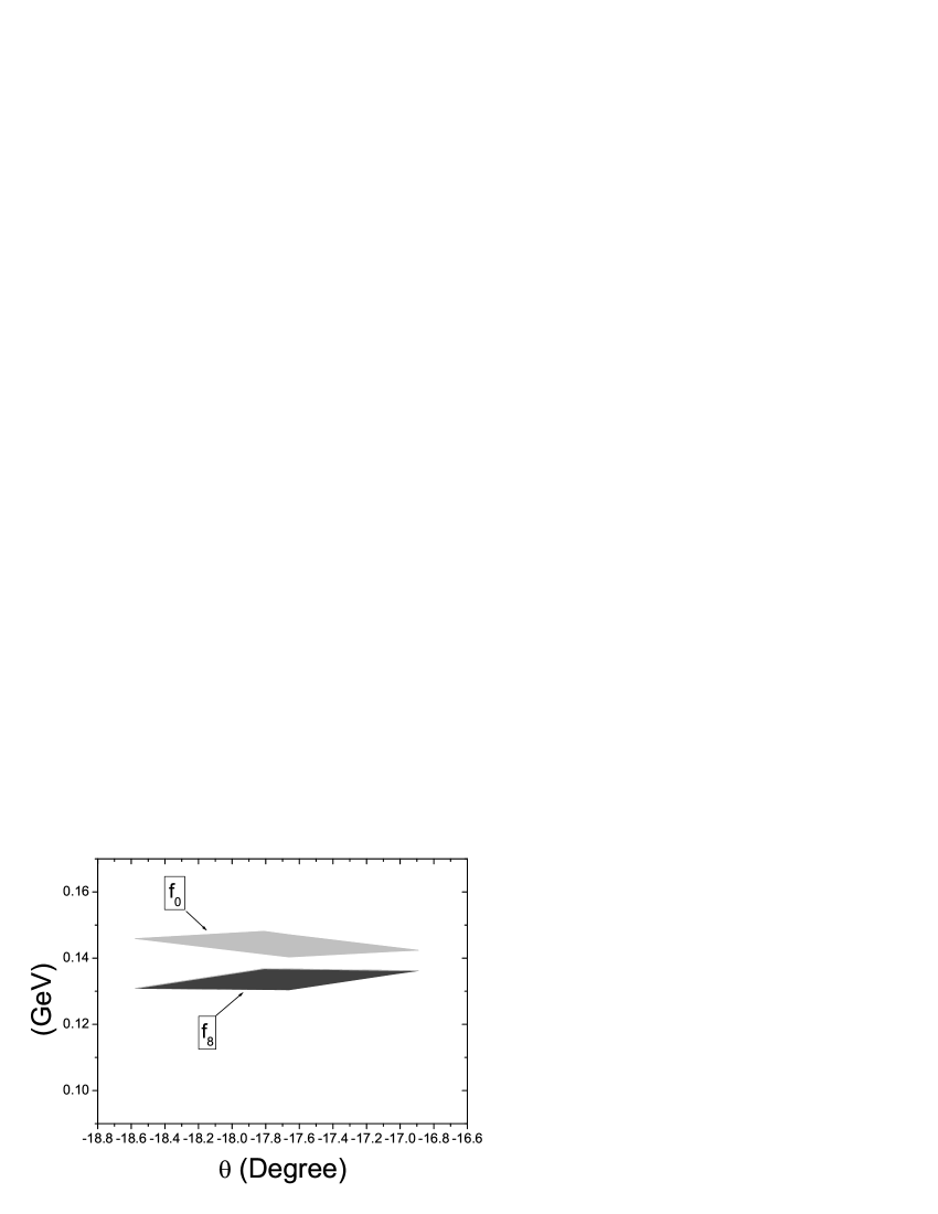
Figure 1: The dependence of $f_{0}$ and $f_{8}$ on $\theta$. The ranges are due to one $\sigma$ errors of data points.

So far the parameter $f_{G_{p}}$ is not well understood. To obtain some information, we use the QCD sum rules to calculate it. The basic idea of QCD sum rule analysis in the present case is to match the dispersion relation involving the hadronic spectral density $\rho(s)$ to the vacuum topological susceptibility $T(-q^{2})=i\int d^{4}xe^{iq\cdot x}\langle 0|T[j_{ps}(x)j_{ps}(0)]|0\rangle$ with the result found by using the operator product expansion. We follow Ref.hhh by making a Borel transformation on $T(s)$ with $\int^{\infty}_{0}Im(T(s)e^{-s/M^{2}}ds/s$ and $\int^{\infty}_{0}Im(T(s))e^{-s/M^{2}}ds$, and including the two ground pseudoscalar states $\eta$ and $\eta^{\prime}$, and $G_{p}$ in the resonant spectral density, to obtain the leading order matching conditionshhh

$$f^{2}_{G_{p}}m^{2}_{G_{p}}e^{-m^{2}_{G_{p}}/M^{2}}+f^{2}_{\eta}m^{2}_{\eta}e^{-m^{2}_{\eta}/M^{2}}+f^{2}_{\eta^{\prime}}m^{2}_{\eta^{\prime}}e^{-m^{2}_{\eta^{\prime}}/M^{2}}$$

$$=\int^{s_{1}}_{0}bse^{-s/M^{2}}ds+\tilde{D}_{4}+O({1\over M^{2}})+inst.,$$

$$f^{2}_{G_{p}}m^{4}_{G_{p}}e^{-m^{2}_{G_{p}}/M^{2}}+f^{2}_{\eta}m^{4}_{\eta}e^{-m^{2}_{\eta}/M^{2}}+f^{4}_{\eta^{\prime}}m^{2}_{\eta^{\prime}}e^{-m^{2}_{\eta^{\prime}}/M^{2}}$$

$$=\int^{s_{1}}_{0}bs^{2}e^{-s/M^{2}}ds-\tilde{D}_{6}+O({1\over M^{2}})+inst.,$$ (4)

where “inst” indicates direct instanton effectsinstanton . $\tilde{D}_{4,6}$ are related to the gluon condensations, $D_{4}=4\langle 0|G_{\mu\nu}G^{\mu\nu}|0\rangle$, and $D_{6}=8g_{s}f_{abc}\langle 0|G^{a}_{\mu\alpha}G^{b,\alpha}_{\nu}G^{c,\nu\mu}|0\rangle$, with $\tilde{D}_{4}=\pi(3\alpha_{s}/4\pi)^{2}D_{4}$, $\tilde{D}_{6}=\pi(3\alpha_{s}/4\pi)^{2}D_{6}$. $b=(3\alpha_{s}/4\pi)^{2}(2/\pi)(1+5\alpha_{s}/\pi)$. In our numerical evaluations, we will use $\langle 0|\alpha_{s}G^{2}|0\rangle=(7.1\pm 0.9)\times 10^{-2}$ GeV⁴ and the relation $\langle 0|g^{3}f_{abc}G^{a}G^{b}G^{c}|0\rangle=1.2\;\mathrm{GeV}^{2}\langle 0|\alpha_{s}G^{2}|0\rangle$ D46 . We comment that there are other $0^{-+}$ states around 1400 MeV region which may contribute to the spectrum density if these states contain large two gluon contents. We will assume that the gluon contents are small in these states and their contributions to the spectrum density can be neglected.

To determine $f_{G_{p}}$, we take the usual practice to find the parameters $f_{G_{p}}$ and $s_{1}$ for a given Borel parameter $M$ and look for a region where the dependence of $f_{G_{p}}$ and $s_{1}$ on $M$ is insensitive. We will negelct the direct instanton effect in our calculation and will come back to comment on the effects later. Note that the analysis with a fixed $G_{p}$ mass here is different than previous onesgmass ; hhh ; D46 where the mass of $G_{p}$ is taken as one of the parameters to be determined and therefore the results is in general different. The solutions for $f_{G_{p}}$ depend on the value $\alpha_{s}$ which we take to be the value at the scale $\mu=m_{G_{p}}$ with $\alpha_{s}=0.35\pm 0.05$. We find that solutions exist only for a restricted parameter space for $\alpha_{s}$ and $\tilde{D}_{4,6}$. In certain ranges, for a given set of input values of $\alpha_{s}$ and $\tilde{D}_{4,6}$, there are two solutions. For example with $\alpha_{s}=0.39$, $\tilde{D}_{4}=1.99\times 10^{-2}\;\mathrm{GeV}^{4}$ and $\tilde{D}_{6}=3.79\times 10^{-3}\;\mathrm{GeV}^{6}$, we get the two solutions to be: a) $s_{1}=3.2$ GeV² and $f_{G_{p}}=0.081$ GeV, and b) $s_{1}=3.5$ GeV² and $f_{G_{p}}=0.091$ GeV. When $M$ is larger than $7$ GeV, the solutions are fairly stable. As long as we choose an $M$ far above $m_{G_{p}}$, the power corrections from higher dimensional operators on the right hand sides of eq. (4) can be suppressed. We note that for the solution with lower $s_{1}$, the value of $s_{1}$ is smaller than $m^{2}_{G_{p}}$ which cannot be considered to be a good solution since it implies that the continuum already starts to contribute to the sum rules in the resonant region in contradiction with the QCD sum rules assumptions. We therefore should choose the solution with the larger $s_{1}$. This solution allows a small gap between the resonances and the continuum. We show the results in Fig. 2 allowing $\alpha_{s}$ to vary from 0.3626 (where solution begins to exist) to $0.4$ (the one $\sigma$ allowed upper bound), and all other quantities, $\tilde{D}_{4,6}$, $f_{\eta,\eta^{\prime}}$ and $\theta$ to vary within one $\sigma$ error ranges. We see that the dependence on $M$ is very mild. We conclude that there are consistent solutions from QCD sum rules for a pseudoscalar of mass 1833.7 MeV, and obtain a conservative range for $f_{G_{p}}$ with

$$f_{G_{p}}=0.072\sim 0.100\;\mbox{GeV}.$$ (5)

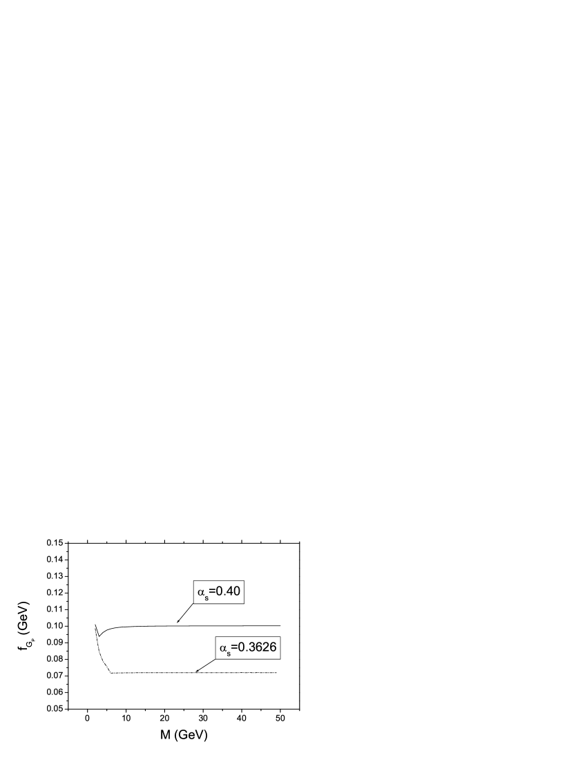
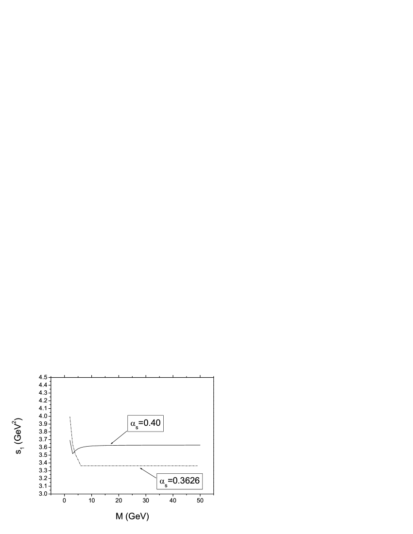
Figure 2: $f_{G_{p}}$ and $s_{1}$ as functions of $M$. The upper and lower bounds are for one $\sigma$ ranges of $\tilde{D}_{4,6}$, $f_{\eta,\eta^{\prime}}$ and $\theta$ with $\alpha_{s}=0.4$ and $\alpha_{s}=0.3626$, respectively.

When we obtained the range of $f_{G_{p}}$, the direct instanton effects were neglected. At large $Q$, the instanton effects are suppressedgmass ; newwork2 ; suppression , for example spike distribution for instanton density results in an exponential suppression when $Q^{2}$ becomes larger than a GeV² or sogmass . With the glueball mass fixed at 1835 MeV, the suppression may not be sufficient to neglect the contributions from the direct instanton. The effects of direct instanton may be substantial. However the detailed calculations depend on the instanton density and the density shape. A reliable evaluation of the instanton effects is difficult. Nevertheless model calculations show that instanton effects may be important due to modification to the normalization of the Wilson coefficients for the relevant operators. We will not go into the specific details as it is too model dependent. Some detailed discussions for direct instanton effects can be found in Ref.gmass . We emphasize that QCD sum rule results should be taken as an estimate within a factor of two. In our later discussions we will use the range for $f_{G_{p}}$ obtained the above as a reference. Should a more precise value will be determined with some method, one can easily rescale the values accordingly.

With the above range for $f_{G_{p}}$, we find that the matrix element $<0|\alpha_{s}G\tilde{G}|G_{p}>$ is larger than $<0|\alpha_{s}G\tilde{G}|\eta(\eta^{\prime})>$ indicating that $G_{p}$ contains a large gluon content. With $f_{G_{p}}$ determined, we are now able to obtain information on the range for $B(J/\psi\to\gamma G_{p})$ combining eq. (1) and experimental data on $J/\psi\to\gamma\eta(\eta^{\prime})$. We have

$$B(J/\psi\to\gamma G_{p})=(2.61\sim 7.37)\times 10^{-3}.$$ (6)

Using the BES data $B(J/\psi\to\gamma G_{p})B(G_{p}\to\pi^{+}\pi^{-}\eta^{\prime})=(2.2\pm 0.4(stat)\pm 0.4(syst))\times 10^{-4}$, we can therefore also obtain the branching ratio of $G_{p}$ to $\pi^{+}\pi^{-}\eta^{\prime}$ using our estimate of $J/\psi\to\gamma G_{p}$. We have

$$B(G_{p}\to\pi^{+}\pi^{-}\eta^{\prime})=(2.21\sim 10.61)\times 10^{-2}.$$ (7)

The branching ratio for this decay is large, but it does not contradict with known data.

If the enhanced threshold $p\bar{p}$ events in $J/\psi\to\gamma p\bar{p}$ is also due to the same $G_{p}$ state, we can obtain information about the interaction of $G_{p}$ with a proton and anti-proton pair, $L=C_{GB}\bar{p}\gamma_{5}pG_{p}$. Since the mass of $G_{p}$ is slightly below the threshold of two proton mass $2m_{p}$, one cannot simply take $B(J/\psi\to\gamma G_{p}\to\gamma p\bar{p})$ to be equal to $B(J/\psi\to\gamma G_{p})B(G_{p}\to p\bar{p})$. One must consider the off-shell effects of $G_{p}$ in terms of the Breit-Wigner approach. We have

$$B(J/\psi\to\gamma G_{p}\to\gamma p\bar{p})=C^{2}_{GB}{B(J/\psi\to\gamma G_{p})\over 8\pi^{2}}$$ (8)

$$\times\int^{m^{2}_{J/\psi}}_{4m^{2}_{p}}dq^{2}{(1-q^{2}/m^{2}_{J/\psi})^{3}q^{2}\over(1-m^{2}_{G_{p}}/m^{2}_{J/\psi})^{3}}{\sqrt{1-4m^{2}_{p}/q^{2}}\over(q^{2}-m^{2}_{G_{p}})^{2}+\Gamma_{G_{p}}^{2}m^{2}_{G_{p}}}.$$

In the above, we have assumed that $C_{GB}$ does not depend on $q^{2}$ sensitively and has been moved out from the integration sign.

Experimental data on $B(J/\psi\to\gamma G_{p}\to\gamma p\bar{p})=(7.0\pm 0.4^{+1.8}_{-0.8})\times 10^{-5}$ then implies

$$C_{GB}=0.42\sim 0.85.$$ (9)

One sees that threshold enhancement data in $J/\psi\to\gamma p\bar{p}$ can also be consistently explained.

We now discuss how the resonance $G_{p}$ may decay into other particles. As have been pointed out earlier this state has a large gluon contents, it may be a glueball which is a SU(3) singlet. Of course one needs to be more open minded that it may has sizeable mixing with other state. We will take the state $G_{p}$ to be a glueball state and study the consequences from flavor symmetry point of view. One can easily study the branching ratios for $J/\psi\to\gamma G_{p}\to\gamma B\bar{B}$ with $B\bar{B}$ a pair of octet baryons. The mixing effect can be easily implemented by introducing some mixing parameters.

The coupling of a SU(3) singlet $G_{p}$ and octet baryon can be written as $L=C_{GB}G_{p}Tr\bar{B}\gamma_{5}B$ with SU(3) flavor symmetry. In Table 1 we list the ratios of $r(B\bar{B})=B(J/\psi\to\gamma G_{p}\to\gamma B\bar{B})/B(J/\psi\to\gamma G_{p}\to\gamma p\bar{p})$ for possible decay modes. We comment that the $X(1835)$ contributions listed in Table 1 hold as long as the resonance is an SU(3) singlet and does not depend on the size of $C_{GB}$. If the resonance transforms non-trivially under the flavor SU(3) symmetry, the predictions would be differenthelima . In principle experimental measurements of these branching ratios can provide important information about the nature of the resonance. However, the branching ratios for other baryon pair decay modes are much smaller than the branching ratio with a proton and anti-proton pair except the neutron and anti-neutron pair decay mode which is then experimentally difficult to carry out. The usefulness of these decay modes depends on whether, near the resonance region, the resonance contributions dominate over the non-resonance continuum parts which we will comment on later.

$r(\Xi^{0}\bar{\Xi}^{0})$	$1.58\times 10^{-3}$
$r(\Xi^{-}\bar{\Xi}^{-})$	$1.38\times 10^{-3}$
$r(\Sigma^{+}\bar{\Sigma}^{+})$	$1.45\times 10^{-2}$
$r(\Sigma^{0}\bar{\Sigma}^{0})$	$1.38\times 10^{-2}$
$r(\Sigma^{-}\bar{\Sigma}^{-})$	$1.28\times 10^{-2}$
$r(\Lambda\bar{\Lambda})$	$4.23\times 10^{-2}$
$r(n\bar{n})$	$0.96$

Table 1: $r(B\bar{B})$ for different $J/\psi\to\gamma G_{P}\to\gamma B\bar{B}$ decays.

A better test of the mechanism may come from other three meson decay modes of $G_{p}$. To have further information on the branching ratios for $G_{p}$ decay into three meson modes, we here follow Ref. neufeld to use U(3) chiral theory to describe how it couples to known meson particles. Notice that the use of U(3) symmetry will not change our previous discussions on $G_{p}\to B\bar{B}$ results. The reason we use U(3) chiral perturbation theory for the interaction is that it can naturally include many properties of chiral anomaly which our calculations for $f_{i}$ depend on. To the leading order there are four terms which may cause $G_{p}$ to decayneufeld

$$L = ia_{1}\partial_{\mu}G_{p}Tr\left(\Sigma^{\dagger}\partial^{\mu}\Sigma\partial_{\nu}\Sigma^{\dagger}\partial^{\nu}\Sigma\right)$$ (10)

$$+ ia_{2}G_{p}Tr\left((\Sigma^{\dagger}\partial^{2}\Sigma-\partial^{2}\Sigma^{\dagger}\Sigma)\partial_{\nu}\Sigma^{\dagger}\partial^{\nu}\Sigma\right)$$

$$+ ia_{3}G_{p}Tr\left(\chi\Sigma-\Sigma^{\dagger}\chi\right)$$

$$+ ia_{4}G_{p}Tr\left(\chi\Sigma^{\dagger}\partial_{\nu}\Sigma\partial^{\nu}\Sigma^{\dagger}-\chi\Sigma\partial_{\nu}\Sigma^{\dagger}\partial^{\nu}\Sigma\right),$$

where $\Sigma=exp[-i\sqrt{2}M/f]$ with $f=f_{\pi}/\sqrt{2}$ and $M$ is the U(3) meson nonet. $\chi$ is proportional to the light quark masses and is given by $\chi=diag(m^{2}_{\pi},m^{2}_{\pi},2m^{2}_{K}-m^{2}_{\pi})$. The last two terms in eq. (10) comes from explicit U(3) (and SU(3)) breaking due to quark masses.

The two SU(3) breaking terms in eq. (10), if dominant, will lead to the main decay mode to be $G_{p}\to\pi KK$neufeld with a very suppressed rate for $G_{p}\to\pi^{+}\pi^{-}\eta^{\prime}$. The BES data indicates that the decay mode $G_{p}\to\pi^{+}\pi^{-}\eta^{\prime}$ has a large branching ratio compared with other three particle decays (yet to be discovered), therefore, these two terms may be suppressed. If the first two terms dominate, we obtain the effective Lagrangian for the decay amplitude $G_{p}\to\pi^{+}\pi^{-}\eta^{\prime}$ to be,

$$L = {4\over\sqrt{3}f^{3}}(\sqrt{2}\cos\theta+\sin\theta)\left(a_{1}\partial_{\mu}G_{p}(\partial^{\mu}\eta^{\prime}\partial_{\nu}\pi^{+}\partial^{\nu}\pi^{-}\right.$$ (11)

$$+ \left.\partial^{\mu}\pi^{-}\partial_{\nu}\pi^{+}\partial^{\nu}\eta^{\prime}+\partial^{\mu}\pi^{+}\partial_{\nu}\eta^{\prime}\partial^{\nu}\pi^{-})\right.$$

$$+ \left.a_{2}G_{p}(\partial^{2}\eta^{\prime}\partial_{\nu}\pi^{+}\partial^{\nu}\pi^{-}+\partial^{2}\pi^{-}\partial_{\nu}\pi^{+}\partial^{\nu}\eta^{\prime}\right.$$

$$+ \left.\partial^{2}\pi^{+}\partial_{\nu}\eta^{\prime}\partial^{\nu}\pi^{-})\right).$$

which leads to a decay amplitude,

$$M(G_{p}\to\pi^{+}\pi^{-}\eta^{\prime})={\sqrt{2}\cos\theta+\sin\theta\over\sqrt{3}f^{3}}$$

$$\times\left(a_{1}[(s-m^{2}_{G_{p}}-m^{2}_{\eta^{\prime}})(s-2m^{2}_{\pi})\right.$$

$$\left.+(t-m^{2}_{G_{p}}-m^{2}_{\pi})(t-m^{2}_{\eta^{\prime}}-m^{2}_{\pi})\right.$$

$$\left.+(u-m^{2}_{G_{p}}-m^{2}_{\pi})(u-m^{2}_{\eta^{\prime}}-m^{2}_{\pi})]\right.$$

$$\left.+2a_{2}[m^{2}_{\eta^{\prime}}(s-2m^{2}_{\pi})+m^{2}_{\pi}(t-m^{2}_{\eta^{\prime}}-m^{2}_{\pi})\right.$$

$$\left.+m^{2}_{\pi}(u-m^{2}_{\eta^{\prime}}-m^{2}_{\pi})]\right),$$ (12)

where $s=(p_{\pi^{+}}+p_{\pi^{-}})^{2}$, $t=(p_{\pi^{-}}+p_{\eta^{\prime}})^{2}$ and $u=(p_{\pi^{+}}+p_{\eta^{\prime}})^{2}$.

To obtain the BES result for $J/\psi\to\gamma\pi^{+}\pi^{-}\eta^{\prime}$ with the $B(J/\psi\to\gamma G_{p})$ obtained earlier, we have

$$|a_{1}|^{2}-0.376Re(a_{1}a_{2}^{*})+0.038|a_{2}|^{2}=(0.94\sim 4.52)\times 10^{-5}\mbox{GeV}^{-2}.$$ (13)

Since there are two parameters, $a_{1}$ and $a_{2}$, involved, with data from $J/\psi\to\gamma G_{p}\to\gamma\pi^{+}\pi^{-}\eta^{\prime}$ alone it is not possible to predict branching ratios for other three meson decay modes. There are several kinematically allowed decay modes which can provide more information. These additional decay modes include: $\eta^{\prime}\pi^{0}\pi^{0}$, $\eta\pi^{+}\pi^{-}$, $\eta\pi^{0}\pi^{0}$, $\eta K^{+}K^{-}$, $\eta K^{0}\bar{K}^{0}$, $\pi^{0}K^{0}\bar{K}^{0}$, $\pi^{0}K^{+}K^{-}$, $\pi^{+}K^{0}K^{-}$, $\pi^{-}\bar{K}^{0}K^{+}$, and $\eta\eta\eta$. With the assumption that the dominant contributions come from the $a_{1,2}$ terms, even with SU(3) breaking effects from the final meson mass differences, one would have the following relations between branching ratios: $B(\pi^{0}\pi^{0}\eta^{\prime}(\eta))=B(\pi^{+}\pi^{-}\eta^{\prime}(\eta))/2$, $B(K^{+}K^{-}\eta)=B(K^{0}\bar{K}^{0}\eta)$, and $B(\pi^{0}K^{+}K^{-})=B(\pi^{0}K^{0}\bar{K}^{0})=B(\pi^{-}K^{+}\bar{K}^{0})/2=B(\pi^{+}K^{-}K^{0})/2$. We list the ratios $r(p_{1}p_{2}p_{3})=B(G_{p}\to p_{1}p_{2}p_{3})/B(G_{p}\to\pi^{+}\pi^{-}\eta^{\prime})$ in Table 2. The branching ratio for $G_{p}\to\pi^{+}\pi^{-}\eta$ can be larger than that for $G_{p}\to\pi^{+}\pi^{-}\eta^{\prime}$. No observation of $J/\psi\to\gamma\pi^{+}\pi^{-}\eta$ near the resonance would imply that there may be large cancellations between terms proportional to $a_{1}$ and $a_{2}$ for this decay mode. $G_{p}\to\pi KK$ are some another modes which may have large branching ratios near the resonance. The branching ratios here are different from those predicted if the resonance transforms non-trivially under the SU(3) symmetrynewwork1 . These new decay modes can serve to test the mechanism proposed in this paper. We urge the BES collaboration to carry out an systematic analysis to obtain more information about the properties of the resonant state $X(1835)$.

$r(\pi^{+}\pi^{-}\eta)$	$11.26(|a_{1}|^{2}-0.186Re(a_{1}a_{2}^{*})+0.009|a_{2}|^{2})/b(\pi^{+}\pi^{-}\eta^{\prime})$
$r(K^{+}K^{-}\eta)$	$1.57\times 10^{-3}(|a_{1}|^{2}-0.474Re(a_{1}a_{2}^{*})+0.056|a_{2}|^{2})/b(\pi^{+}\pi^{-}\eta^{\prime})$
$r(K^{+}K^{-}\pi^{0})$	$2.47(|a_{1}|^{2}-0.291Re(a_{1}a_{2}^{*})+0.021|a_{2}|^{2})/b(\pi^{+}\pi^{-}\eta^{\prime})$
$r(\eta\eta\eta)$	$0.006(|a_{1}|^{2}-0.538Re(a_{1}a_{2}^{*})+0.073|a_{2}|^{2})/b(\pi^{+}\pi^{-}\eta^{\prime})$

Table 2: $r(p_{1}p_{2}p_{3})$ for various $G_{p}\to p_{1}p_{2}p_{3}$ decay modes. Here $b(\pi^{+}\pi^{-}\eta^{\prime})=|a_{1}|^{2}-0.376Re(a_{1}a_{2}^{*})+0.038|a_{2}|^{2}$.

In the above discussions about predictions for other decay modes, only contributions from the resonance are included. There are also non-resonance effects. To isolate the resonance contributions near the resonance region, one should remove the off-resonance contributions by extrapolating the data away the resonance to the resonance region. Theoretical study of the non-resonance contributions is more complicated. We briefly discuss how the non-resonance contributions for $J/\psi\to\gamma B\bar{B}$ and $J/\psi\to\gamma\pi^{+}\pi^{-}\eta(\eta^{\prime})$ can be parameterized using SU(3) flavor symmetry. The general form for non-resonance $J/\psi\to\gamma B\bar{B}$ has been discussed in Ref.helima . As far as the SU(3) structure is concerned, that is, neglecting Lorentz structure, we have the amplitudes for non-resonance contributions to $J/\psi\to\gamma B\bar{B}$ and $J/\psi\to p_{1}p_{2}p_{3}$ to be given by

$$M(J/\psi\to\gamma B\bar{B})\sim Tr[\bar{B}(D_{\gamma}\{Q,B\}+F_{\gamma}[Q,B])],$$

$$M(J/\psi\to\gamma p_{1}p_{2}p_{3})\sim\tilde{a}\eta_{1}Tr(QM^{2})++\tilde{b}\eta_{1}\eta_{1}Tr(QM)+\tilde{c}Tr(QM^{3}).$$ (14)

where $Q=diag(2/3,-1/3,-1/3)$ is the electric charge matrix. $D_{\gamma}$, $F_{\gamma}$, $\tilde{a}$, $\tilde{b}$ and $\tilde{c}$ are form factors.

The complications in extracting information on the form factors $D_{\gamma}$ and $F_{\gamma}$, and, $\tilde{a}$, $\tilde{b}$ and $\tilde{c}$ are two folds. One of them is that the Lorentz structure is much more complicated, that is for each of the form factors $D_{\gamma}$, $F_{\gamma}$, $\tilde{a}$ and $\tilde{b}$, there are actually several of them depending on how the Dirac matrices are inserted in the $B\bar{B}$ bi-baryon product, and how derivatives are taken on the meson and baryon fields. Another is that the form factors in general depend on combinations of the invariant masses of pairs of particles in the final state. Nevertheless, fitting data, one can obtain information about the parameters. Measurements of branching ratios of $J/\psi\to\gamma B\bar{B},\gamma p_{1}p_{2}p_{3}$ via non-resonance can also provide important information for understanding the whole physics picture.

In summary, we have studied some implications of a possible $0^{-+}$ resonance in the $\pi^{+}\pi^{-}\eta^{\prime}$ spectrum in $J/\psi\to\gamma\pi^{+}\pi^{-}\eta^{\prime}$ observed by BES. We have shown that it has a sizeable matrix element for $<0|G\tilde{G}|G_{p}>$. The branching ratios for $J/\psi\to\gamma G_{p}$ and $G_{p}\to\pi^{+}\pi^{-}\eta^{\prime}$, using QCD anomaly and QCD sum rules, are determined to be $(2.61\sim 7.37)\times 10^{-3}$ and $(2.21\sim 10.61)\times 10^{-2}$, respectively. The coupling for $G_{p}-p-\bar{p}$ interaction is also determined. We conclude that a pseudoscalar $0^{-+}$ with large gluon content can consistently explain the data. We have also studied branching ratios of other decay modes using SU(3) flavor symmetry. We find that $J/\psi\to\gamma G_{p}\to\gamma(\pi^{+}\pi^{-}\eta,KK\pi^{0})$ can provide useful tests for the mechanism proposed here.

Acknowledgments We thank N. Kochelev and S. Narison for useful discussions. X.G.H thanks B. McKellar for hospitality at the University of Melbourne while part of this work was carried out. This work was supported in part by grants from NSC and NNSFC (10421003).

References

(1) M. Ablikim et al., BES Collaboration,
Phys. Rev. Lett. 95, 262001 (2005).
(2) J. Z. Bai et al., BES Collaboration, Phys. Rev. Lett.
91, 022001 (2003).
(3) For a recent reveiw see J. Rosner,
hep-ph/0508155.
(4) J. Rosner, Phys. Rev. D 68, 014004 (2003);
A. Datta and P. O’connell, Phys. Lett. B 567, 273 (2003); B.S.
Zou and H.C. Chiang, Phys. Rev. D 69, 034004 (2004); X. Liu et
al., High Energy Phys. Nucl. Phys. 30, 1 (2006); C.H. Chang
and H.R. Pang, Commun. Theor. Phys. 43, 275 (2005); A.
Sibirtsev et al., Phys. Rev. D 71, 054010 (2005); H. Loiseau
and S. Wyceck, Phys. Rev. C 72, 011001 (2005); M.L. Yan et
al., Phys. Rev. D 72, 034027 (2005); G.J. Ding and M.L. Yan,
Phys. Rev. C 72, 015208 (2005); S.L. Zhu and C.S. Gao, Commun.
Theor. Phys. 46, 291 (2006).
(5) N. Kochelev and D.P. Min, Phys. Lett. B 633, 283 (2006).
(6) S. Narison,
Nucl. Phys. B 509, 312 (1998); H. Forkel, Phys. Rev. D71, 054008 (2005).
(7) G. Gabadadze, Phys. Rev. D 58, 055003 (1998);
X.G. He, W.S. Hou and C.S. Huang, Phys. Lett. B 429, 99
(1998).
(8) C.J. Morningstar and M. Peardon,
Phys. Rev. D 60, 034509 (1999);
A. Hart and M. Teper, Phys. Rev. D 65,
34502 (2002).
(9)
V. A. Novikov, M. A. Shifman, A. I. Vainshtein and V. I. Zakharov,
Nucl. Phys. B 165, 55 (1979).
(10) J.P. Ma, Nucl. Phys. B 605, 625 (2001), Erratum-ibid, B611, 523 (2001);
Phys. Rev. D 65, 097506 (2002); X.G. He, H.Y. Jin and J.P. Ma,
Phys. Rev. D 66, 074015 (2002).
(11) F. Close, G. Farrar and Z.P. Li, Phys. Rev. D 55, 5749 (1997).
(12) P. Ball, J.M. Frere and M. Tytgat, Phys. Lett. B
365, 367 (1996); R. Akhoury, J.M. Frere, Phys. Lett. B 220,
258 (1989); K.T. Chao, Nucl. Phys. B 317, 597 (1989).
(13) S. Eidelman et al., Particle Data Group, Phys. Lett.
B 592, 1 (2004).
(14) P. Ball, J.M. Frere and M. Tytgat in
anomaly ; A. Bramon, R. Ecribano and M.D. Scadron, Eur. Phys.
J. C 7, 271 (1999).
(15) V.A. Novikov et al., Nucl. Phys. B 191, 301 (1981).
(16)
T. Huang, H.Y. Jin and A.L. Zhang, Phys. Rev. D 59, 4026
(1999) ; S. Narison, Nucl. Phys. B 502, 312 (1998).
(17) V. A. Novikov et al., Phys. Lett. B 86, 347 (1979).
(18) X.G. He, X.Q. Li and J.P. Ma, Phys. Rev. D 71, 014031 (2005).
(19) G. Gounaris and H. Neufeld, Phys. Lett. B213, 541 (1988), Erratum-ibid. B 218, 508 (1989).