Diquark-Antidiquark with open charm in QCD sum rules

Abstract

Using the QCD sum rule approach we investigate the possible four-quark structure of the recently observed charmed scalar mesons $D_{0}^{0}(2308)$ (BELLE) and $D_{0}^{0,+}(2405)$ (FOCUS) and also of the very narrow $D_{sJ}^{+}(2317)$, firstly observed by BABAR. We use diquak-antidiquark currents and work to the order of $m_{s}$ in full QCD, without relying on $1/m_{c}$ expansion. Our results indicate that a four-quark structure is acceptable for the resonances observed by BELLE and BABAR: $D_{0}^{0}(2308)$ and $D_{sJ}^{+}(2317)$ respectively, but not for the resonances observed by FOCUS: $D_{0}^{0,+}(2405)$.

In general, the classification of mesons containing a single heavy quark is interpreted with the help of heavy-quark symmetry, i.e., the symmetry valid for the infinitely heavy mass of charm quark. Under this symmetry, the strong interaction conserves total angular momentum of the light quark, $j$. In the meanwhile, total angular momentum of the light-heavy system, $J$, should be still regarded as a good quantum number of the system, even if the heavy-quark symmetry breaks down. In this way, the classification of the charmed mesons can be explained in terms of the quantum numbers $(L,S,J,j)$, where $L$ and $S$ denote the orbital angular momentum between the light and heavy quarks and total spin of the system, respectively. The doublets with $j=1/2$ and $L=0$ have been observed over the past two decades ($\sim 1975~{}-~{}1994)$ following the discovery of open charm, because these states have relatively narrow widths. Recently the first observations of the scalar charmed mesons $(j=1/2,~{}L=1)$ have been reported. The very narrow $D_{sJ}^{+}(2317)$ was first discovered in the $D_{s}^{+}\pi^{0}$ channel by the BABAR Collaboration babar and its existence was confirmed by CLEO cleo , BELLE belle1 and FOCUS focus Collaborations. Its mass was commonly measured as $2317\nobreak\,\mbox{MeV}$, which is approximately $160\nobreak\,\mbox{MeV}$ below the prediction of the very successful quark model for the charmed mesons god . The BELLE Collaboration belle2 has also reported the observation of a rather broad scalar meson $D_{0}^{0}(2308)$, and the FOCUS Collaboration focus2 reported evidence for broad structures in both neutral and charged final states that, if interpreted as resonances in the $J^{P}=0^{+}$ channel, would be the $D_{0}^{0}(2407)$ and the $D_{0}^{+}(2403)$ mesons. While the mass of the scalar meson, $D_{0}^{0}(2308)$, observed by BELLE Collaboration is also bellow the prediction of ref. god (approximately $100\nobreak\,\mbox{MeV}$), the masses of the states observed by FOCUS Collaboration are in complete agreement with ref. god .

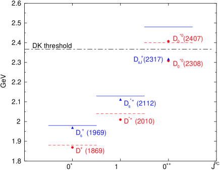
Figure 1: Spectroscopy of the pseudoscalar, vector and scalar charmed mesons.The theoretical predictions of ref. god are represented as solid lines for the $c\bar{s}$ and dashed lines for the $c\bar{q}$, and the experimental data are represented as triangles for the $c\bar{s}$ and circles for the $c\bar{q}$.

The spectroscopy of $c\bar{q}$ and $c\bar{s}$ pseudoscalar, vector and scalar mesons is drawn in Fig. 1, where the theoretical predictions of ref. god are represented as solid lines for the $c\bar{s}$ and dashed lines for the $c\bar{q}$, and the experimental data are represented as triangles for the $c\bar{s}$ and circles for the $c\bar{q}$.

Due to its low mass, the structure of the meson $D_{sJ}^{+}(2317)$ has been extensively debated. It has been interpreted as a $c\bar{s}$ state dhlz ; bali ; ukqcd ; ht ; nari , two-meson molecular state bcl ; szc , $D-K$- mixing br , four-quark states ch ; tera ; mppr or a mixture between two-meson and four-quark states bpp . The same analyses would also apply to the meson $D_{0}^{0}(2308)$.

In the light sector the idea that the light scalar mesons (the isoscalars $\sigma(500),~{}f_{0}(980)$, the isodublet $\kappa(800)$ E791 and the isovector $a_{0}(980)$) could be four-quark bound states is not new jaffe ; cloto . Indeed, in a four-quark scenario, the mass degeneracy of $f_{0}(980)$ and $a_{0}(980)$ is natural, the mass hierarchy pattern of the nonet is understandable, and it is easy to explain why $\sigma$ and $\kappa$ are broader than $f_{0}(980)$ and $a_{0}(980)$. The decays $\sigma\to\pi\pi$, $\kappa\to K\pi$ and $f_{0},~{}a_{0}\to KK$ are OZI superallowed without the need of any gluon exchange, while $f_{0}\to\pi\pi$ and $a_{0}\to\eta\pi$ are OZI allowed as it is mediated by one gluon exchange. Since $f_{0}(980)$ and $a_{0}(980)$ are very close to the $\bar{K}K$ threshold, the $f_{0}(980)$ is dominated by the $\pi\pi$ state and $a_{0}(980)$ is governed by the $\eta\pi$ state. Consequently, they are narrower than $\sigma$ and $\kappa$.

In this work we use the method of QCD sum rules (QCDSR) svz to study the two-point functions of the scalar mesons, $D_{sJ}(2317)$, $D_{0}(2308)$ and $D_{0}(2405)$ considered as four-quark states. In a recent calculation sca the light scalar mesons were considered as $S$-wave bound states of a diquark-antidiquark pair. As suggested in ref. jawil the diquark was taken to be a spin zero colour anti-triplet. We extend this prescription to the charm sector and, therefore, the corresponding interpolating fields containing zero, one and two strange quarks are:

$$j_{0} = \epsilon_{abc}\epsilon_{dec}(q_{a}^{T}C\gamma_{5}c_{b})(\bar{u}_{d}\gamma_{5}C\bar{d}_{e}^{T}),$$

$$j_{1} = {\epsilon_{abc}\epsilon_{dec}\over\sqrt{2}}\left[(u_{a}^{T}C\gamma_{5}c_{b})(\bar{u}_{d}\gamma_{5}C\bar{s}_{e}^{T})+u\leftrightarrow d\right],$$

$$j_{2} = \epsilon_{abc}\epsilon_{dec}(s_{a}^{T}C\gamma_{5}c_{b})(\bar{q}_{d}\gamma_{5}C\bar{s}_{e}^{T}),$$ (1)

where $q$ represents the quark $u$ or $d$ according to the charge of the meson. Since $D_{sJ}$ has one $\bar{s}$ quark, we choose the $j_{1}$ current to have the same quantum numbers of $D_{sJ}$, which is supposed to be an isoscalar. However, since we are working in the SU(2) limit, the isoscalar and isovector states are mass degenerate and, therefore, this particular choice has no relevance here.

The QCDSR for the charmed scalar mesons with $n$ strange quarks are constructed from the two-point correlation function

$$\Pi(q)=i\int d^{4}x~{}e^{iq.x}\langle 0|T[j_{n}(x)j^{\dagger}_{n}(0)]|0\rangle.$$ (2)

In the OPE side we work at leading order and consider condensates up to dimension six. We deal with the strange quark as a light one and consider the diagrams up to order $m_{s}$. To keep the charm quark mass finite, we use the momentum-space expression for the charm quark propagator. We calculate the light quark part of the correlation function in the coordinate-space, which is then Fourier transformed to the momentum space in $D$ dimensions. The resulting light-quark part is combined with the charm-quark part before it is dimensionally regularized at $D=4$.

We can write the correlation function in the OPE side in terms of a dispersion relation:

$$\Pi^{OPE}(q^{2})=\int_{m_{c}^{2}}^{\infty}ds{\rho(s)\over s-q^{2}}\;,$$ (3)

where the spectral density is given by the imaginary part of the correlation function: $\rho(s)={1\over\pi}\mbox{Im}[\Pi^{OPE}(s)]$.

In the phenomenological side, the coupling of the scalar meson with $n$ strange quarks, $S_{n}$, to the scalar current, $j_{n}$, can be parametrized in terms of the meson decay constant $f_{S_{n}}$ as sca : $\langle 0|j_{n}|S_{n}\rangle=\sqrt{2}f_{S_{n}}m_{S_{n}}^{4}$, therefore, the phenomenological side of Eq. (2) can be written as

$$\Pi^{phen}(q^{2})={2f_{S_{n}}^{2}m_{S_{n}}^{8}\over m_{S_{n}}^{2}-q^{2}}+\cdots\;,$$ (4)

where the dots denote higher resonance contributions that will be parametrized, as usual, through the introduction of the continuum threshold parameter $s_{0}$ io1 . After making a Borel transform on both sides, and transferring the continuum contribution to the OPE side, the sum rule for the scalar meson $S_{n}$ can be written as

$$2f_{S_{n}}^{2}m_{S_{n}}^{8}e^{-m_{S_{n}}^{2}/M^{2}}=\int_{m_{c}^{2}}^{s_{0}}ds~{}e^{-s/M^{2}}~{}\rho_{S_{n}}(s)\;,$$ (5)

where $\rho_{S_{n}}(s)=\rho^{pert}(s)+\rho^{m_{s}}(s)+\rho^{\langle\bar{q}q\rangle}(s)+\rho^{\langle G^{2}\rangle}(s)+\rho^{mix}(s)+\rho^{\langle\bar{q}q\rangle^{2}}(s)+\rho^{\langle G^{3}\rangle}(s)$, with blmnn

$$\rho^{pert}(s)={1\over 2^{10}3\pi^{6}}\int_{\Lambda}^{1}d\alpha\left({1-\alpha\over\alpha}\right)^{3}(m_{c}^{2}-s\alpha)^{4},$$ (6)

$$\rho^{\langle G^{2}\rangle}(s)={\langle g^{2}G^{2}\rangle\over 2^{10}\pi^{6}}\int_{\Lambda}^{1}d\alpha~{}(m_{c}^{2}-s\alpha)\bigg{[}{m_{c}^{2}\over 9}$$

$$\times\left({1-\alpha\over\alpha}\right)^{3}+(m_{c}^{2}-s\alpha)\left({1-\alpha\over 2\alpha}+{(1-\alpha)^{2}\over 4\alpha^{2}}\right)\bigg{]},$$ (7)

$$\rho^{\langle G^{3}\rangle}(s)={\langle g^{3}G^{3}\rangle\over 2^{12}9\pi^{6}}\int_{\Lambda}^{1}d\alpha\left({1-\alpha\over\alpha}\right)^{3}(3m_{c}^{2}-s\alpha),$$ (8)

which are common to all three resonances and where the lower limit of the integrations is given by $\Lambda=m_{c}^{2}/s$. From $j_{0}$ we get: $\rho^{m_{s}}(s)=0$,

$$\rho^{\langle\bar{q}q\rangle}(s)=-{m_{c}\langle\bar{q}q\rangle\over 2^{6}\pi^{4}}\int_{\Lambda}^{1}d\alpha\left({1-\alpha\over\alpha}\right)^{2}(m_{c}^{2}-s\alpha)^{2},$$ (9)

$$\rho^{mix}(s)={m_{c}\langle\bar{q}g\sigma.Gq\rangle\over 2^{6}\pi^{4}}\bigg{[}{1\over 2}\int_{\Lambda}^{1}d\alpha\left({1-\alpha\over\alpha}\right)^{2}$$ (10)

$$\times (m_{c}^{2}-s\alpha)-\int_{\Lambda}^{1}d\alpha{1-\alpha\over\alpha}(m_{c}^{2}-s\alpha)\bigg{]},$$

$$\rho^{\langle\bar{q}q\rangle^{2}}(s)=-{\langle\bar{q}q\rangle^{2}\over 12\pi^{2}}\int_{\Lambda}^{1}d\alpha~{}(m_{c}^{2}-s\alpha).$$ (11)

From $j_{1}$ we get: $\rho^{m_{s}}(s)=0$,

$$\rho^{\langle\bar{q}q\rangle}(s)={1\over 2^{6}\pi^{4}}\int_{\Lambda}^{1}d\alpha~{}{1-\alpha\over\alpha}(m_{c}^{2}-s\alpha)^{2}\bigg{[}$$

$$-\langle\bar{q}q\rangle\left(2m_{s}+m_{c}{1-\alpha\over\alpha}\right)+m_{s}\langle\bar{s}s\rangle\bigg{]},$$ (12)

$$\rho^{mix}(s) = {1\over 2^{6}\pi^{4}}\int_{\Lambda}^{1}d\alpha~{}(m_{c}^{2}-s\alpha)\bigg{[}-{m_{s}\langle\bar{s}g\sigma.Gs\rangle\over 6}$$ (13)

$$+ \langle\bar{q}g\sigma.Gq\rangle\bigg{(}-m_{s}(1-\ln(1-\alpha))$$

$$- m_{c}{1-\alpha\over\alpha}\left(1-{1\over 2}{1-\alpha\over\alpha}\right)\bigg{)}\bigg{]}$$

$$\rho^{\langle\bar{q}q\rangle^{2}}(s)=-{\langle\bar{q}q\rangle\langle\bar{s}s\rangle\over 12\pi^{2}}\int_{\Lambda}^{1}d\alpha~{}(m_{c}^{2}-s\alpha).$$ (14)

Finally from $j_{2}$ we get

$$\rho^{m_{s}}(s)=-{m_{s}m_{c}\over 2^{8}3\pi^{6}}\int_{\Lambda}^{1}d\alpha\left({1-\alpha\over\alpha}\right)^{3}(m_{c}^{2}-s\alpha)^{3},$$ (15)

$$\rho^{\langle\bar{q}q\rangle}(s)={1\over 2^{6}\pi^{4}}\int_{\Lambda}^{1}d\alpha{1-\alpha\over\alpha}(m_{c}^{2}-s\alpha)^{2}\bigg{[}$$

$$\langle\bar{s}s\rangle\left(2m_{s}-m_{c}{1-\alpha\over\alpha}\right)-2m_{s}\langle\bar{q}q\rangle\bigg{]},$$ (16)

$$\rho^{mix}(s)={1\over 2^{6}\pi^{4}}\int_{\Lambda}^{1}d\alpha~{}(m_{c}^{2}-s\alpha)\bigg{[}{\langle\bar{s}g\sigma.Gs\rangle\over 2}$$ (17)

$$\times \bigg{(}{m_{s}\over 3}-m_{s}{1-\alpha\over\alpha}-m_{c}{1-\alpha\over\alpha}\left(1-{1\over 2}{1-\alpha\over\alpha}\right)\bigg{)}$$

$$- m_{s}\langle\bar{q}g\sigma.Gq\rangle(1-\ln(1-\alpha))\bigg{]},$$

$$\rho^{\langle\bar{q}q\rangle^{2}}(s)=-{\langle\bar{q}q\rangle\langle\bar{s}s\rangle\over 12\pi^{2}}\int_{\Lambda}^{1}d\alpha~{}(m_{c}^{2}-s\alpha).$$ (18)

In the numerical analysis of the sum rules, the values used for the quark masses and condensates are: $m_{s}=0.13\,\nobreak\,\mbox{GeV}$, $m_{c}=1.2\,\nobreak\,\mbox{GeV}$, $\langle\bar{q}q\rangle=\,-(0.23)^{3}\,\nobreak\,\mbox{GeV}^{3}$, $\langle\overline{s}s\rangle\,=0.8\langle\bar{q}q\rangle$, $\langle\bar{q}g\sigma.Gq\rangle=m_{0}^{2}\langle\bar{q}q\rangle$ with $m_{0}^{2}=0.8\,\nobreak\,\mbox{GeV}^{2}$, $\langle g^{2}G^{2}\rangle=0.5~{}\nobreak\,\mbox{GeV}^{4}$ and $\langle g^{3}G^{3}\rangle=0.045~{}\nobreak\,\mbox{GeV}^{6}$.

We call $D_{0}^{(0s)}$, $D_{0}^{(1s)}$ and $D_{0}^{(2s)}$ the scalar charmed mesons represented by $j_{0}$, $j_{1}$ and $j_{2}$ (in Eq. (1)) respectively.

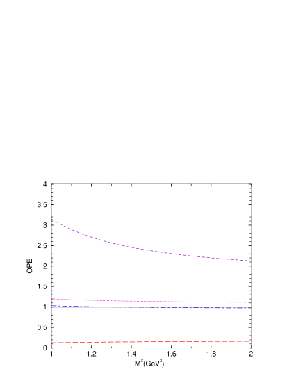
Figure 2: Borel mass dependence of the relative contributions of the OPE terms: perturbative (long-dashed line), perturbative plus quark condensate (dot-dashed line), previous plus four-quark condensate (dashed line), previous plus mixed condensate (solid line).

In Fig. 2 we show, as a function of the Borel mass, the OPE relative contribution of the: perturbative (long-dashed line), perturbative plus quark condensate (dot-dashed line), previous plus four-quark condensate (dashed line) and previous plus mixed condensate (solid line), for the $D_{0}^{(1s)}$ meson. We see that there is no good OPE convergence and that the four-quark condensate and the mixed condensate contributions are very big, as compared with the perturbative contribution, and with opposite signal, in such a way that the final result is almost the same as before adding these two contributions. One can argue that this is not a good sum rule, since there is not a good OPE convergence. We notice, however, that this is a common feature of the sum rules for currents with more than three quarks. The thre-gluon condensate contribution is negligible for all three currents and this is why we do not show it in Fig. 2. The same behaviour is obtained for $D_{0}^{(0s)}$ and $D_{0}^{(2s)}$ mesons.

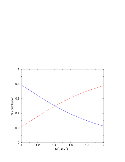
Figure 3: Borel mass dependence of the relative contributions of the pole (solid line) and continuum (dashed line) contributions.

In Fig. 3 we show, as a function of the Borel mass, the percentage of the pole and continuum contributions to the total contribution for the $D_{0}^{(1s)}$ meson. We see that in the Borel window $1.0\nobreak\,\mbox{GeV}^{2}\leq M^{2}\leq 1.4\nobreak\,\mbox{GeV}^{2}$ the pole contribution is always bigger than the continuum contribution. Therefore, this is the Borel window that we will consider.

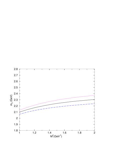
Figure 4: The $D_{0}^{(0s)}$ mass as a function of the Borel mass for different values of the continuum threshold. Dashed line: $\sqrt{s_{0}}=2.6\nobreak\,\mbox{GeV}$; solid line: $\sqrt{s_{0}}=2.7\nobreak\,\mbox{GeV}$; dotted line: $\sqrt{s_{0}}=2.8\nobreak\,\mbox{GeV}$.

In order to get rid of the meson decay constant and extract the resonance mass, $m_{S_{n}}$, we first take the derivative of Eq. (5) with respect to $1/M^{2}$ and then we divide it by Eq. (5) to get

$$m_{S_{n}}^{2}={\int_{m_{c}^{2}}^{s_{0}}ds~{}e^{-s/M^{2}}~{}s~{}\rho_{S_{n}}(s)\over\int_{m_{c}^{2}}^{s_{0}}ds~{}e^{-s/M^{2}}~{}\rho_{S_{n}}(s)}\;.$$ (19)

In Figs. 4 and 5 we show the masses of the $D_{0}^{(0s)}$ and $D_{0}^{(1s)}$ resonances, respectively, as a function of the Borel mass for different values of the continuum threshold. The results for the $D_{0}^{(2s)}$ resonance is similar to that for the $D_{0}^{(1s)}$ resonance, as shown in ref.blmnn .

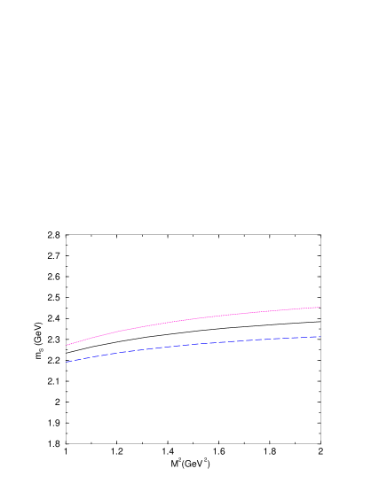
Figure 5: The $D_{0}^{(1s)}$ mass as a function of the Borel mass for different values of the continuum threshold. Dashed line: $\sqrt{s_{0}}=2.6\nobreak\,\mbox{GeV}$; solid line: $\sqrt{s_{0}}=2.7\nobreak\,\mbox{GeV}$; dotted line: $\sqrt{s_{0}}=2.8\nobreak\,\mbox{GeV}$.

Comparing these two figures we see that the mass of $D_{0}^{(0s)}$ is around $100\nobreak\,\mbox{MeV}$ smaller than the others, since the $D_{0}^{(1s)}$ and $D_{0}^{(2s)}$ resonance masses are basicaly degenerated blmnn . While it is natural to expect that the inclusion of a strange quark would increase the resonance mass by around the strange quark mass (as was the case when one goes from $D_{0}^{(0s)}$ to $D_{0}^{(1s)}$), it is really interesting to observe that this does not happen when one goes from $D_{0}^{(1s)}$ to $D_{0}^{(2s)}$. In terms of the OPE contributions, we can trace this behavior to the fact that the quark condensate term is smaller in $D_{0}^{(2s)}$ than in $D_{0}^{(1s)}$ (due to the change from $m_{c}\langle\bar{q}q\rangle$ to $m_{c}\langle\bar{s}s\rangle$), however the inclusion of the term proportional to $m_{s}m_{c}$ (which is not present in $D_{0}^{(1s)}$), compensates this decrease.

Considering the variations on the quark masses and on the continuum threshold discussed above, in the Borel window considered here our results for the ressonance masses are given in Table I.

Table I: Numerical results for the resonance masses

resonance	$D_{0}^{(0s)}$	$D_{0}^{(1s)}$	$D_{0}^{(2s)}$
mass (GeV)	$2.22\pm 0.15$	$2.32\pm 0.13$	$2.31\pm 0.14$

Comparing the results in Table I with the resonance masses given by BABAR, BELLE and FOCUS: $D_{sJ}^{+}(2317)$, $D_{0}^{0}(2308)$ and $D_{0}^{0,+}(2405)$, we see that we can identify the four-quark states represented by $D_{0}^{(1s)}$ and $D_{0}^{(2s)}$ with the BABAR and BELLE resonances respectively. However, we do not find a four-quark state whose mass is compatible with the FOCUS resonances, $D_{0}^{0,+}(2405)$. Therefore, we associate the FOCUS resonances, $D_{0}^{0,+}(2405)$, with a scalar $c\bar{q}$ state, since its mass is completly in agreement with the predictions of the quark model in ref. god . It is also interesting to point out that a mass of about $2.4~{}\nobreak\,\mbox{GeV}$ is also compatible with the the QCD sum rule calculation for a $c\bar{q}$ scalar meson ht .

One can argue that while a pole approximation is justified for the very narrow BABAR resonance, this may not be the case for the rather broad BELLE and FOCUS resonances. To check if the width of the resonances could modify the pattern observed in the masses of the four-quark states, in ref.blmnn the phenomenological side of the sum rule, in Eq. (5), was modified through the introduction of a Breit-Wigner-type resonance form do02 . It was shown that the best agreement between the right-hand and left-hand sides of the sum rule is obtained for $m_{S}\sim 2.2~{}\nobreak\,\mbox{GeV}$. Therefore our conclusion is that the inclusion of the width does not change the value of the mass obtained for the resonance.

Besides de masses, another important point to understand the nature of the charmed meson states is their corresponding decay width. One can ask how, in the present approach, it is possible to obtain a extremely narrow width for $D_{sJ}^{+}(2317)$, while the $D_{0}^{0}(2308)$ state remain fairly wide? To compute the decay width of the hadronic decay ${D_{0}^{(1s)}}\to D_{s}^{+}\pi^{0}$, for example, one has to study the three-point function

$$T_{\mu}(p,p^{\prime},q)=\int d^{4}x~{}d^{4}y~{}e^{i.p^{\prime}.x}~{}e^{iq.y}$$

$$\times\langle 0|T\{j_{D_{s}}(x)j_{5\mu}^{\pi}(y)j_{1}^{\dagger}(0)\}|0\rangle,$$ (20)

where $p=p^{\prime}+q$, and the currents for the two pseudoscalar mesons in the vertex are

$$j_{5\mu}^{\pi} = {1\over\sqrt{2}}(\bar{u}_{a}\gamma_{\mu}\gamma_{5}u_{a}-\bar{d}_{a}\gamma_{\mu}\gamma_{5}d_{a}),$$

$$j_{D_{s}} = i\bar{s}_{a}\gamma_{5}c_{a}.$$ (21)

In the phenomenological side, the three-point function in Eq. (20) is related with the vertex coupling constant, $g_{D_{0}^{(1s)}D_{s}\pi}$, which is related with the decay width through the relation:

$$\Gamma(D_{0}^{(1s)}\rightarrow D_{s}\pi)=$$

$${1\over 16\pi m_{S_{1}}^{3}}g_{D_{0}^{(1s)}D_{s}\pi}^{2}\sqrt{\lambda(m_{S_{1}}^{2},m_{D_{s}}^{2},m_{\pi}^{2})},$$ (22)

where $\lambda(a,b,c)=a^{2}+b^{2}+c^{2}-2ab-2ac-2bc$.

For the light scalar mesons considered as diquark- antidiquark states, the study of their decay width using the QCD sum rule approach was done in ref.sca . In Table II we show the results obtained for the different vertices studied in ref. sca , as well as the experimental values.

Table II: Numerical results for the coupling constants

vertex	$g(\nobreak\,\mbox{GeV})$	$g^{exp}(\nobreak\,\mbox{GeV})$
$\sigma\pi^{+}\pi^{-}$	$3.1\pm 0.5$	$2.6\pm 0.2$
$\kappa K^{+}\pi^{-}$	$3.6\pm 0.3$	$4.5\pm 0.4$
$f_{0}K^{+}K^{-}$	$1.6\pm 0.1$
$f_{0}\pi^{+}\pi^{-}$	$0.47\pm 0.05$	$1.6\pm 0.8$

From Table II we see that, although not exactly in between the experimental error bars, the hadronic couplings determined from the QCD sum rule calculation are consistent with existing experimental data. The biggest discrepancy is for $g_{f_{0}\pi^{+}\pi^{-}}$ and this can be understood since the $f_{0}\to\pi^{+}\pi^{-}$ decay is mediated by one gluon exchange and, therefore, probably in this case $\alpha_{s}$ corrections could play an important role. In the case of the decay $f_{0}(a_{0})\rightarrow K^{+}K^{-}$, the coupling can not be experimentally measured due to the lack of phase space.

In the case of the decay ${D_{0}^{(1s)}}\to D_{s}^{+}\pi^{0}$, for an isoscalar ${D_{0}^{(1s)}}$, in the QCD sum rule approach one only gets a result different from zero for the coupling constant, if one allows a break in the $SU(2)$ symmetry. In this case, the coupling is proportional to the difference of the masses of the $u$ and $d$ quarks, and the difference of the $u$ and $d$ quark condensates. In a preliminary calculation we got

$$g_{D_{0}^{(1s)}D_{s}\pi}\sim 0.06\nobreak\,\mbox{GeV},$$ (23)

which gives a decay width $\Gamma(D_{0}^{(1s)}\rightarrow D_{s}\pi)\sim 8$ KeV. It is important to notice that, if we have used a isovector current for the $D_{0}^{(1s)}$ state instead of an isoscalar current, we would get $\Gamma(D_{0}^{(1s)}\rightarrow D_{s}\pi)\sim 260~{}\nobreak\,\mbox{MeV}$. Therefore, it seems possible, in this four-quark scenario, to obtain a extremely narrow width for $D_{sJ}^{+}(2317)$, while the $D_{0}^{0}(2308)$ state remain fairly wide.

In conclusion, we have presented a QCD sum rule study of the charmed scalar mesons considered as diquark-antidiquark states. We found that the masses of the BABAR, $D_{sJ}^{+}(2317)$, and BELLE, $D_{0}^{0}(2308)$, resonances can be reproduced by the four-quark states $(cq)(\bar{q}\bar{s})$ and $(cs)(\bar{u}\bar{s})$ respectively. However, the mass of the FOCUS resonance, $D_{0}^{0,+}(2405)$ can not be reproduced in the four-quark state picture considered here. Therefore, we interpret it as a normal $c\bar{q}$ state, since its mass is in complete agreement with the predictions of the quark model in ref. god . We also obtain a mass of $\sim 2.2~{}\nobreak\,\mbox{GeV}$ for a four-quark scalar state $(cq)(\bar{u}\bar{d})$ which was not yet observed, and that should be also rather broad.

References

(1) BABAR Coll., B. Auber et al., Phys. Rev. Lett.
90, 242001 (2003); Phys. Rev. D69, 031101 (2004).
(2) CLEO Coll., D. Besson et al., Phys. Rev. D68,
032002 (2003).
(3) BELLE Coll., P. Krokovny et al., Phys. Rev. Lett.
91, 262002 (2003).
(4) FOCUS Coll., E.W. Vaandering, hep-ex/0406044.
(5) S. Godfrey and N. Isgur, Phys. Rev. D32, 189 (1985);
S. Godfrey and R. Kokoshi, Phys. Rev. D43, 1679 (1991).
(6) BELLE Coll., K. Abe et al., Phys. Rev. D69,
112002 (2004).
(7) FOCUS Coll., J.M. Link et al., Phys. Lett.
B586, 11 (2004).
(8) Y.-B. Dai, C.-S. Huang, C. Liu and S.-L. Zhu,
Phys. Rev. D68, 114011 (2003).
(9) G.S. Bali, Phys. Rev. D68, 071501(R) (2003).
(10) A. Dougall, R.D. Kenway, C.M. Maynard and C. Mc-Neile,
Phys. Lett. B569, 41 (2003).
(11) A. Hayashigaki and K. Terasaki, hep-ph/0411285.
(12) S. Narison, Phys. Lett. B605, 319 (2005).
(13) T. Barnes, F.E. Close and H.J. Lipkin, Phys. Rev. D68,
054006 (2003).
(14) A.P. Szczepaniak, Phys. Lett. B567, 23 (2003).
(15) E. van Beveren and G. Rupp, Phys. Rev. Lett. 91,
012003 (2003).
(16) H.-Y. Cheng and W.-S. Hou, Phys. Lett. B566, 193 (2003).
(17) K. Terasaki, Phys. Rev. D68, 011501(R) (2003).
(18) L. Maiani, F. Piccinini, A.D. Polosa, V. Riquer,
Phys. Rev. D71, 014028 (2005).
(19) T. Browder, S. Pakvasa and A.A. Petrov, Phys. Lett.
B578, 365 (2004).