Next-to-leading order QCD jet production with parton showers and hadronization

Abstract

We report on a method for matching the next-to-leading order calculation of QCD jet production in $e^{+}e^{-}$ annihilation with a Monte Carlo parton shower event generator (MC) to produce realistic final states. The final result is accurate to next-to-leading order (NLO) for infrared-safe one-scale quantities, such as the Durham 3-jet fraction $y_{3}$, and agrees well with parton shower results for multi-scale quantities, such as the jet mass distribution in 3-jet events. For our numerical results, the NLO calculation is matched to the event generator Pythia, though the method is more general. We compare one scale and multi-scale quantities from pure NLO, pure MC, and matched NLO-MC calculations.

I Introduction

Perturbation theory is the basic tool for deriving predictions for experiment from the standard model and its extensions. When some of the particles feel the strong interaction, a perturbative expansion in powers of the strong coupling $\alpha_{s}$ can be employed. As long as a short-distance process is involved, the reasonably small value ($\alpha_{s}\sim 1/10$) of the running strong coupling justifies such an expansion, and the leading term is a good first approximation. However, the estimated error to a leading order (LO) prediction (that is, the error that one estimates from leaving out all of the higher order terms) is often so large that one wants a next-to-leading order (NLO) calculation. In fact, next-to-leading order predictions are available in the form of computer programs for a wide variety of processes for electron-positron collisions, electron-hadron collisions, and hadron-hadron collisions. The essential limitation is on the number of partons involved in the hard interaction. Thus $p+p\to W+2\ {\it jets}+X$ is available at next-to-leading order while $p+p\to W+3\ {\it jets}+X$ is not.

A typical next-to-leading order calculation predicts the expectation value $\langle{\cal S}\rangle$ of an “infrared-safe” observable ${\cal S}$ in the style of an event generator. That is, the program generates a large number $N$ of events characterized by their final states $f_{n}$, with each event having a weight $w_{n}$. Letting the value of ${\cal S}$ for state $f_{n}$ be ${\cal S}(f_{\!n})$, the calculated expectation value of ${\cal S}$ is

$$\langle{\cal S}\rangle={1\over N}\sum_{n=1}^{N}w_{n}\,{\cal S}(f_{\!n})\;.$$ (1)

(A convenient normalization is $(1/N)\sum_{n=1}^{N}w_{n}=1$ so that $\langle{1}\rangle=1$. One could also take $\langle{1}\rangle=\sigma_{\rm tot}$.) The quantity $\langle{\cal S}\rangle$ has the perturbative expansion

$$\langle{\cal S}\rangle=C_{0}({\cal S})\,\alpha_{s}^{B}+C_{1}({\cal S})\,\alpha_{s}^{B+1}+C_{2}({\cal S})\,\alpha_{s}^{B+2}+\cdots\;,$$ (2)

where B is the power of $\alpha_{s}$ in the lowest-order graph for $\langle{\cal S}\rangle$. The numerical result of the NLO calculation is not exact, but produces the first two terms of this expansion.

Typical programs that do next-to-leading order calculations suffer from a serious deficiency: the final states $f_{n}$ are not realistic. First of all, they consist of just a few partons. In the case of $e^{+}+e^{-}\to 3\ {\it jets}$, which we consider in this paper, the final states consist of a quark, an antiquark, and one gluon or else a quark, an antiquark, and two gluons or another quark-antiquark pair. This is not the kind of state that can be used directly as input to a detector simulation.

The situation is even worse than might be deduced from the fact that the final states consist of few partons instead of (many) hadrons. At its core, an NLO calculation depends on the use of an infrared-safe inclusive observable since it depends on a cancellation of divergences associated with different numbers of on-shell partons. As a concrete example, consider the fraction of events in $e^{+}+e^{-}\to{\it hadrons}$ that contain precisely three jets as determined by the $k_{T}$ (or Durham) algorithm kTjets with $y_{\rm cut}=0.05$. Call this fraction $f_{3}$. We have

$$\langle f_{3}\rangle=C_{0}(f_{3})\,\alpha_{s}+C_{1}(f_{3})\,\alpha_{s}^{2}+C_{2}(f_{3})\,\alpha_{s}^{3}+\cdots\;.$$ (3)

A next-to-leading order program can accurately predict $C_{0}$ and $C_{1}$. Now suppose that we use the program to determine the differential three-jet fraction $df_{3}/dM$, where $M$ is the mass of one of the jets (so that each event contributes three entries for $df_{3}/dM$ and $\int\!dM\,df_{3}/dM=3f_{3}$). Even if one is ultimately interested in $f_{3}$, it is reasonable to be interested in predicting this more detailed quantity, because a realistic detector may respond differently to narrow and wide jets and we may be concerned with how much detector effects influence the measurement. Now, one can expect the NLO result to be approximately correct for $df_{3}/dM$ as long as $M$ is large, but for $M/\sqrt{s}\ll 1$, a sophisticated user will expect a pure NLO program to give an answer that is not physically realistic. We illustrate what goes wrong by simply plotting the result for $f_{3}^{-1}\,df_{3}/dM$ versus $M$ from a purely NLO program in Fig. 1. We see that $f_{3}^{-1}\,df_{3}/dM$ becomes large for small $M$ and that the fraction of events in the first bin is large and negative. As $M\to 0$, $df_{3}/dM$ according to the NLO calculation develops a $\log(M)/M$ singularity together with a term proportional to $\delta(M)$ with an infinite negative coefficient. The integral $f_{3}=(1/3)\int\!dM\,df_{3}/dM$ of this highly singular function gives an accurate estimate of the three-jet fraction $f_{3}$ but the differential distribution is completely unphysical. In fact, it requires a binning of the distribution even to get finite numbers. A much more realistic expectation for $f_{3}^{-1}\,df_{3}/dM$ can be obtained by using a parton shower Monte Carlo event generator Pythia ; Herwig ; Ariadne . Recall that the shower Monte Carlo programs add up a series of logarithmic terms, approximating the behavior of Feynman graphs near the singularities corresponding to collinear parton splitting or soft gluon emission. The prediction of the shower Monte Carlo Pythia Pythia for $f_{3}^{-1}\,df_{3}/dM$ is shown in Fig. 2 and is compared to the NLO calculation. We see that the NLO perturbative calculation agrees qualitatively with Pythia for large $M$, but fails for small $M$.

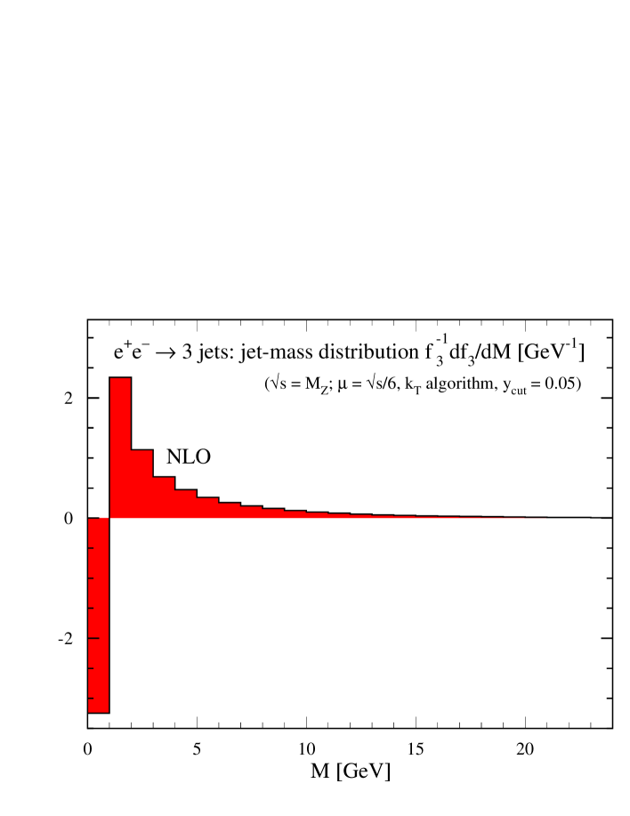
Figure 1: Jet mass distribution in three-jet events, $f_{3}^{-1}\,df_{3}/dM$, calculated at next-to-leading order for $\sqrt{s}=M_{Z}$. The three jets are identified using the $k_{T}$ algorithm with $y_{\rm cut}=0.05$. Then $M$ is the invariant mass of one of the three jets, with each event making three contributions to $df_{3}/dM$. The renormalization scale is chosen as $\mu=\sqrt{s}/6$ and $\alpha_{s}(M_{Z})=0.118$. This is a pure NLO calculation using beowulf . There is a large negative contribution in the first bin.

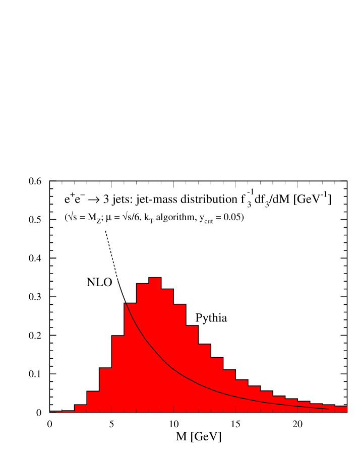
Figure 2: Jet mass distribution in three-jet events, $f_{3}^{-1}\,df_{3}/dM$, calculated according to Pythia Pythia with default parameters for $\sqrt{s}=M_{Z}$. The cross section is defined as in Fig. 1. The jet mass distribution from the perturbative NLO calculation in Fig. 1 is shown for comparison.

Clearly if one were interested in how the differential response of a detector to wide and narrow jets would affect a measurement of $f_{3}$, one would be better off using Pythia than the NLO program, even though Pythia has only leading-order accuracy for $f_{3}=(1/3)\int\!dM\,df_{3}/dM$. However, would it not be better to add parton showering and hadronization according to Pythia to the NLO calculation? That is the topic discussed in this paper.

There has been substantial recent progress in adding a parton shower and hadronization to an NLO calculation. Frixione, Nason and Webber FrixioneWebberI ; FrixioneWebberII ; FrixioneWebberIII ; Nason:2004rx have presented and implemented an algorithm that makes use of the shower Monte Carlo program Herwig Herwig to do NLO calculations for a selection of processes for which there are two hadrons in the initial state and at leading order the final state particles that carry color are massive. Processes available include the hadroproduction of single vector and Higgs bosons, vector boson pairs, heavy quark pairs, and lepton pairs. Two of the present authors have described an algorithm for a process with massless color carrying particles in the final state, namely $e^{+}+e^{-}\to 3\ {\it jets}$ nloshowersI ; nloshowersII . This algorithm was implemented with an NLO calculation coupled to a small self-contained shower generator with no hadronization.

The calculations of Refs. nloshowersI ; nloshowersII sufficed to demonstrate the principles of the algorithm, but for practical purposes one would like to have a shower algorithm that has been tested against data (as in Herwig and Pythia) and one would like to include hadronization. For this reason, we present here results from coupling the program described in Refs. nloshowersI ; nloshowersII to the standard shower Monte Carlo program Pythia, including its hadronization following the Lund string model. The code described here is available at the site beowulfcode . Other work on this general subject can be found in Refs. otherwork .

II Sketch of the algorithm

The general algorithm that we use to couple an NLO program for $e^{+}+e^{-}\to 3\ {\it jets}$ to a shower Monte Carlo is described in some detail in Refs. nloshowersI ; nloshowersII , so we present just a sketch here. Specific details about the coupling to Pythia that go beyond Refs. nloshowersI ; nloshowersII are described in the following section.

Consider first the Born graphs. A quark-antiquark-gluon state is generated with a weight proportional to one of the Born graphs times the complex conjugate of one of the Born graphs. Each of these partons splits into two with a probability described by a splitting function and a Sudakov exponential that represents the probability not to have split at a higher virtuality. This splitting is called a primary splitting and is represented by the square vertices in Fig. 3. The splitting functions have the right singularities to represent the collinear limit of QCD matrix elements and the collinear $\times$ soft limit, but they are not correct in the limit of the emission of a wide angle soft gluon. Accordingly, we generate a gluon emission with a weight that matches the matrix element for the radiation of a very soft gluon from the antenna produced by the three outgoing partons. This emission is represented by the gluon in Fig. 3, which is drawn to suggest that it is emitted from the outgoing partons as a whole but not from any particular one of them.

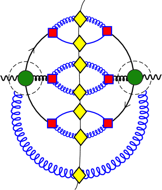
Figure 3: Parton splitting in Refs. nloshowersI ; nloshowersII . The filled circles represent graphs for the Born amplitude and complex conjugate amplitude. Each of the partons emerging from the Born amplitude splits into two partons with a vertex, represented by the squares, that includes a Sudakov suppression factor. The extra gluon coming from the circles on the right and left represents the soft gluon radiated from the three jets. Each of the seven daughter partons undergoes further, secondary, splittings according to Pythia and enters the final state as a complete shower with hadronization. The secondary splittings are represented by the diamonds.

Next, the seven parton final state thus generated is modified somewhat as described in the following section and fed to Pythia, which creates a complete shower and hadronization. We have modified Pythia slightly so that it is able to accept a partially developed shower and generate suitably narrow jets from each of the seven partons. We outline the required modifications in the following section.

The splitting incorporated in the Born graphs has two important features. First, when the virtuality $\bar{q}^{2}$ of the pair of daughter partons is small, the splitting probability is proportional to $(P(x)/\bar{q}^{2})d\bar{q}^{2}dx$ where $x$ is the share of the momentum carried by one of the daughter partons and $P(x)$ is the appropriate Altarelli-Parisi splitting function. Second, the collinear singularity at $\bar{q}^{2}\to 0$ is damped by a Sudakov factor with the behavior $\exp(-\alpha_{s}\,c\log^{2}(\bar{q}^{2}))$ for $\bar{q}^{2}\to 0$. Thus each of the three original partons makes a jet, but in the limit of small $\alpha_{s}$, each jet is usually very narrow and appears in an infrared-safe measurement like a single massless parton. There is a qualifying adverb “usually” here. A fraction $\alpha_{s}$ of the time, one of the splittings has a substantial virtuality and we get a four-jet final state. Thus there is an order $\alpha_{s}^{B+1}$ effect in which some probability is removed from the three-jet final state and given to a four-jet final state. In a purely NLO calculation, this effect is included in the $\alpha_{s}^{B+1}$ graphs. Since we do not want any part of the order $\alpha_{s}^{B+1}$ contribution to be counted twice, we need to subtract these terms from the $\alpha_{s}^{B+1}$ graphs. One of these subtraction terms is illustrated in Fig. 4. The subtraction terms have the effect of removing collinear and soft divergences from the order $\alpha_{s}^{B+1}$ graphs.

In addition to the Born graphs, there are subtracted order $\alpha_{s}^{B+1}$ graph with either three or four partons in the final state. Each of the final state partons from these graphs is fed to Pythia, which creates a complete shower and hadronization using appropriate initial conditions as described in the following section. This showering is represented by the diamonds in Fig. 4.

Figure 4: Treatment of order $\alpha_{s}^{B+1}$ graphs. One particular cut diagram is shown, in this case a cut diagram with a virtual loop. The second diagram illustrates a subtraction term, which corresponds to a contribution at order $\alpha_{s}^{B+1}$ from Fig. 3. The partonic final state is generated with a weight proportional to the difference of matrix elements, then this final state is sent to Pythia, which is represented by the diamonds.

The Sudakov suppression factors play an important role in the primary showering that takes place before the partons are passed to Pythia. In the case of quark splitting, the Sudakov factor has the form

$$\exp\left(-\int_{\bar{q}^{2}}^{\infty}\frac{d\bar{l}^{2}}{l^{2}}\int_{0}^{1}dz\ \frac{\alpha_{s}}{2\pi}\,{\cal P}_{g/q}(\bar{l}^{2},z,|\vec{q}^{\,2}|)\right)\;,$$

where $\bar{q}^{2}$ is the virtuality of the splitting and $\vec{q}$ is the momentum of the parent quark. The function ${\cal P}_{g/q}(\bar{l}^{2},z)$ represents “virtual” splittings and is derived from the one loop quark self-energy graph in the Coulomb gauge. It reduces to the usual Altarelli-Parisi splitting function in the limit $\bar{l}^{2}\to 0$ at fixed $z$. However the usual $1/z$ singularity is absent, being cut off for $z<\bar{l}^{2}/|\vec{q}^{\,2}|$, where $\vec{q}$ is the momentum of the mother quark. The integration over $z$ produces a logarithm of $\bar{l}^{2}/|\vec{q}^{\,2}|$. Then the integration over $\bar{l}^{2}$ produces a second logarithm so that splitting at very small $\bar{q}^{2}$ is suppressed by a Sudakov factor that is, in a first approximation, $\exp(-\alpha_{s}\,c\log^{2}(\bar{q}^{2}))$. In Refs. nloshowersI ; nloshowersII , the Sudakov factor is not derived as a summation of logarithms. Rather, it is derived as a useful way of expressing the effect of virtual graphs on small $\bar{q}^{2}$ splittings. Compare this to the standard perturbative treatment of small $\bar{q}^{2}$ splittings in which large positive probabilities from real parton emissions are counterbalanced by large negative probabilities from virtual parton graphs. With the Sudakov factor, we avoid the small $\bar{q}^{2}$ singularities: we suppress them with an exponential factor. When expanded in powers of $\alpha_{s}$, the result is the same as given by the standard perturbative calculation. Next, one simply notes that the Sudakov suppression factor is just what one wants as the first step in a shower Monte Carlo algorithm, where this factor appears as a way of summing logarithms.

This algorithm is based on the order $\alpha_{s}^{B}$ and $\alpha_{s}^{B+1}$ graphs for $e^{+}e^{-}\to 3\ {\it jets}$. It is designed to produce NLO calculations for infrared-safe three-jet observables while, at the same time, providing a reasonably accurate parton shower description for the inner structure of the three jets. Future NLO-MC hybrid programs will likely have a mechanism for switching from a three-jet description to a two-jet description, as in Refs. Catani:2001cc and Mrenna:2003if at lowest order and Ref. Nagy:2005aa at NLO. Such a mechanism is not built into the present program. For this reason, the present program should not be used to calculate observables that receive significant contributions from two-jet final states. In fact, in the program, events that are too close to a two-jet configuration based on the thrust of the perturbative event are simply cut from the calculation.

III Merging with Pythia

In this section, we address the issue of how to pass the perturbative events after primary showering through a standard event generator to include additional jet structure and hadronization. In this paper, we use the Pythia event generator, though there is no limitation (in principle) to using another one.

For some time now, Pythia has been able to perform parton showering and hadronization on externally-generated partonic configurations. This has become technically simpler with the adoption of a general data structure by several Monte Carlo authors lha1 . The parton shower that is added, however, is based on partons that are generated from a hard process at a single scale. We need something different since the further showering of the partonic state sent to Pythia needs to recognize several scales that were involved in generating these partons.

We begin with seven partons from a Born graph as depicted in Fig. 3, three partons from an order $\alpha_{s}^{B+1}$ graph with a virtual loop as depicted in Fig. 4, or four partons from an order $\alpha_{s}^{B+1}$ graph with no virtual loop. These final state partons are generated with flavor identifications $\{g,u,\bar{u},d,\dots\}$ and with labels indicating color connections based on the color structure of the underlying Feynman graphs. (The idea of color connections as used in parton shower Monte Carlo programs neglects terms suppressed by $1/N_{\rm c}^{2}$, where $N_{\rm c}$ is the number of colors, and neglects quantum interference graphs. Thus the assignment of color connections can only be a rough approximation in a calculation with exact color factors for the graphs and with quantum interference included. Nevertheless, an assignment of color connections is needed in order for Pythia to generate string hadronization.) We also supply the quark masses used in Pythia to the final state quarks. The momenta for final state partons were generated in the approximation that all partons are massless, but the momenta are adjusted so that final state quarks are on-shell with the proper masses.

Before the partonic final state is passed to Pythia, a certain amount of analysis is needed.

The first step is to account for the minimum virtuality of 1 ${\rm GeV}^{2}$ allowed in a Pythia shower. In contrast, there are no infrared cutoffs in the virtualities of the parton splittings in Fig. 3 or in the energy of the soft gluon there. Thus in order to generate partonic states that are sensible within the context of Pythia, the program checks whether any of the three splittings indicated in Fig. 3 had a virtuality less than the minimum. If there was an unallowed splitting, the two daughter partons are replaced by the mother parton and the parton is flagged so that it is not showered by Pythia. In addition, if the soft gluon in Fig. 3 (or any other final state gluon that did not arise from a $1\to 2$ splitting) has an energy less than 100 MeV, the gluon is erased and its momentum and color is reassigned to the other partons. This step leaves us with seven or fewer partons to be passed to Pythia.

The next step is to generate a synthetic shower history that could have resulted in the final state partons. This shower history is generated based on the $k_{T}$-algorithm modified to account for the flavors and colors of the final state partons, so that we get a shower history that is allowed in QCD at leading order in $1/N_{\rm c}^{2}$. In generating this shower history, we define the resolution variable to be the LUCLUS resolution variable that is used in Pythia:

$$k_{T,ij}=2(1-\cos\theta_{ij})\ \frac{E_{i}^{2}E_{j}^{2}}{(E_{i}+E_{j})^{2}}\;.$$ (4)

Here the energies and angles are defined in the overall center-of-mass frame of the event. The jet algorithm examines all of the $k_{T,ij}$ values for pairs $\{i,j\}$ of partons that have flavors and color connections that would allow them to be combined. The pair with the smallest $k_{T,ij}$ is combined (by adding their four-momenta). Then the algorithm repeats until, at last, we have just one remaining quark-antiquark pair. We use this synthetic shower history to define, for each final state parton $i$, a certain initial virtuality scale $Q_{i}$, a maximum transverse momentum $k_{T,i}^{\rm max}$, and a maximum angle $\theta_{i}^{\rm max}$. The first splitting generated by Pythia for parton $i$ should have $k_{T}<k_{T,i}^{\rm max}$ and $\theta<\theta_{i}^{\rm max}$.

To define $k_{T,i}^{\rm max}$, we find the $k_{T}$ of the splitting that produced parton $i$ in the synthetic shower history. We define $k_{T,i}^{\rm max}$ to be the lesser of this and a global maximum $k_{T}$, which is the largest $k_{T,ij}$ in the shower. The purpose of using this global scale is to guarantee that the hardest interaction is generated in the perturbative NLO calculation, not by Pythia.

To define $\theta_{i}^{\rm max}$, we find the one or two final state partons $j$ with which parton $i$ is color connected and define $\theta_{i}^{\rm max}=\min_{j}\theta_{ij}$.

To define the initial virtuality scale $Q_{i}$ there are a number of cases. When parton $i$ is a quark or antiquark that can be traced back to the $\gamma^{*}/Z$ vertex, we define $Q_{i}^{2}=s$. When parton $i$ is a quark or antiquark that can be traced back to a $g\to q\bar{q}$ vertex, we define $Q_{i}^{2}=p_{g}^{2}$ where $p_{g}$ is the four-momentum of the gluon at which the quark or antiquark line started. When parton $i$ is a gluon that originated at a $q\to qg$ or $\bar{q}\to\bar{q}g$ vertex, we define $Q_{i}^{2}=p_{\rm m}^{2}$ where $p_{\rm m}$ is the four-momentum of the quark or antiquark that is the mother for the gluon. When parton $i$ is a gluon that originated at a $g\to gg$ vertex and is the less energetic of the two sister gluons, we define $Q_{i}^{2}=p_{\rm m}^{2}$ where $p_{\rm m}$ is the four-momentum of the mother gluon. When parton $i$ is a gluon that originated at a $g\to gg$ vertex and is the more energetic of the two sister gluons, we define $Q_{i}^{2}=p_{\rm mm}$ where $p_{\rm mm}$ is the four-momentum of the grandmother of the gluon.

The idea now is to ask Pythia to generate further showering for each final state parton $i$ according to the standard Pythia splitting kernels, but with the first splitting limited by the requirements $k_{T}<k_{T,i}^{\rm max}$ and $\theta<\theta_{i}^{\rm max}$. In order to incorporate the $k_{T}$ restriction into a shower based on the initial virtuality scale $Q_{i}$, we follow the procedure of Mrenna:2003if , based on the suggestion of Catani:2001cc . The shower for each parton $i$ is started at scale $Q_{i}$ but splittings that do not satisfy $k_{T}<k_{T,i}^{\rm max}$ are ignored (“vetoed”), where $k_{T}$ is the parton shower definition of this quantity, ${k_{T}^{2}}=z(1-z)m^{2}$, using $z$ as the energy fraction of one daughter with respect to the mother of virtuality $m$. Splittings that do not satisfy $\theta<\theta_{i}^{\rm max}$ are also vetoed, as is standard in Pythia. Once a first allowed splitting has been generated, the rest of the shower from parton $i$ is generated according to the normal algorithms of Pythia. After parton showering, Pythia generates hadrons by string fragmentation.

IV Results

In this section, we test the program that combines the NLO calculation with showers and hadronization as sketched in Secs. I and II. We shall refer to this program as NLO+PS+Had. If we use just the Born graphs with showers and hadronization, leaving out the contributions from order $\alpha_{s}^{2}$ graphs, we shall refer to the program as LO+PS+Had. For comparison, we also display results from a pure lowest order perturbative calculation, LO, a pure next-to-leading order perturbative calculation, NLO, and just the Pythia program (version 6.221 with default parameters unless specially noted). Our standard choice for the c.m. energy is $\sqrt{s}=M_{Z}$ with $\alpha_{s}(M_{Z})=0.118$. In the perturbative calculations, we need to choose a renormalization scale. Our default choice is $\mu=\sqrt{s}/6$, based on the observation that in jet production for hadron physics the choice $\mu=E_{T}/2$ works well and in the $e^{+}e^{-}$ case each jet has a typical energy $E\approx\sqrt{s}/3$.

We will first examine the three-jet fraction $f_{3}$ as a function of the jet resolution parameter $y_{\rm cut}$. Here the hope is that $f_{3}[\mbox{\tt NLO+PS+Had}]$ will match $f_{3}[{\tt NLO}]$ reasonably well since $f_{3}[\mbox{\tt NLO+PS+Had}]$ is supposed to be correct to next-to-leading order. Then we will examine $f_{3}^{-1}\,df_{3}/dM$ at a fixed choice for $y_{\rm cut}$, which we take as $y_{\rm cut}=0.05$ (chosen because at this value $f_{3}$ is approximately $1\times\alpha_{s}$). For $f_{3}^{-1}\,df_{3}/dM$ we recall that the pure NLO result is completely unrealistic. The hope is that $f_{3}^{-1}\,df_{3}[\mbox{\tt NLO+PS+Had}]/dM$ will match $f_{3}^{-1}\,df_{3}[{\tt Pythia}]/dM$ reasonably well since Pythia is generally known to give a pretty realistic match to data.

We begin with $f_{3}$ as a function of the jet resolution parameter $y_{\rm cut}$, which we display in Fig. 5. We first note that with our choice of renormalization scale, $f_{3}[{\tt LO}]$ is rather close to $f_{3}[{\tt NLO}]$. This agreement can be taken as a sign that the choice or renormalization scale was sensible.

Next, we note that $f_{3}[\mbox{\tt LO+PS+Had}]$ is quite a lot smaller than $f_{3}[{\tt NLO}]$ or $f_{3}[{\tt LO}]$. What has happened is that the first stage of showering in the algorithm used here changes the normalization by an amount proportional to $\alpha_{s}$. This change is not as alarming as it might seem. For $y_{\rm cut}=0.05$ we have $f_{3}[\mbox{\tt LO+PS+Had}]/f_{3}[{\tt LO}]\approx 0.5$. If we write this as one factor for each jet,

$$\frac{f_{3}[\mbox{\tt LO+PS+Had}]}{f_{3}[{\tt LO}]}=\Big{[}1-X\,\alpha_{s}(\sqrt{s}/6)\Big{]}^{3}$$ (5)

with $\alpha_{s}(\sqrt{s}/6)\approx 0.16$, then the coefficient $X$ is not large, $X\approx 1.5$. One could make $X$ closer to zero by modifying the functions used in the primary showering, as discussed in the last paragraph of Sec. IV of Ref. nloshowersI . For instance one could make the Sudakov exponent smaller. However, we do not attempt such an adjustment in this paper.

We are now ready to look at $f_{3}[\mbox{\tt NLO+PS+Had}]$, for which the correction terms based on order $\alpha_{s}^{2}$ graphs are designed to produce a result that is correct to order $\alpha_{s}^{2}$. Indeed, we see that $f_{3}[\mbox{\tt NLO+PS+Had}]$ matches $f_{3}[{\tt NLO}]$ to about 10%, which is within the error that one expects for a next-to-leading order calculation.

Finally in Fig. 5 we show $f_{3}[{\tt Pythia}]$. We see that $f_{3}[{\tt Pythia}]$ matches $f_{3}[{\tt NLO}]$ quite well, even though Pythia does not contain all the terms needed for next-to-leading order accuracy. On the other hand, Pythia does contain some next-to-leading order terms in the form of its choice of scale and in the generation of showers. Evidently, these terms do quite a good job of approximating the full next-to-leading order result. In fact, one might be inclined to rely entirely on Pythia if it were not for the fact that one cannot really tell how accurate its approximations are without having a full next-to-leading order calculation with which to compare it.

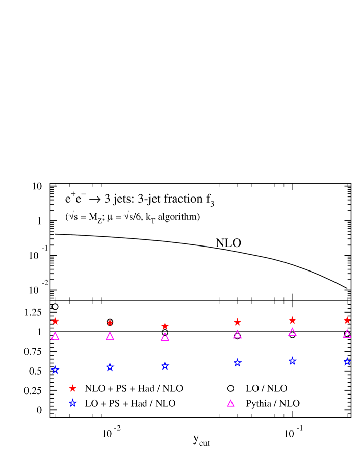
Figure 5: Three-jet fraction, $f_{3}$, versus $y_{\rm cut}$. The top panel shows $f_{3}[{\tt NLO}]$. The bottom panel shows the ratios of $f_{3}[{\tt NLO+PS+Had}]$, $f_{3}[{\tt LO+PS+Had}]$, $f_{3}[{\tt LO}]$, and $f_{3}[{\tt Pythia}]$ to $f_{3}[{\tt NLO}]$. The parameters are as in Figs. 1 and 2.

A more rigorous perturbative test of whether NLO+PS, without hadronization in this case, is indeed correct to next-to-leading order can be obtained by studying the ratio

$$R[\mbox{\tt NLO+PS}]=\frac{f_{3}[\mbox{\tt NLO+PS}]-f_{3}[\mbox{\tt NLO}]}{f_{3}[\mbox{\tt NLO}]}\;.$$ (6)

The difference between $f_{3}[\mbox{\tt NLO+PS}]$ and $f_{3}[\mbox{\tt NLO}]$ should be of order $\alpha_{s}^{3}$ so that the ratio $R$ should have a perturbative expansion that begins at order $\alpha_{s}^{2}$. We can test this by evaluating $f_{3}$ at different c.m. energies $\sqrt{s}$ and plotting the ratio $R$ against $\alpha_{s}^{2}(\sqrt{s})$. The results of this test are shown in the upper panel of Fig. 6 for the c.m. energies $\sqrt{s}=34$ GeV, $M_{Z}$, 500 GeV and 1000 GeV, corresponding to $\alpha_{s}=0.139$, 0.118, 0.0940 and 0.0868, respectively. We see the expected shape of the $R$ curve, which approaches a straight line through the origin as $\alpha_{s}^{2}\to 0$. For comparison, we show the line $R=0.22\,\alpha_{s}^{2}(\sqrt{s})/\alpha_{s}^{2}(M_{Z})$. In the lower panel of Fig. 6 we display the impact of hadronization by plotting the difference $\Delta R=R[\mbox{\tt NLO+PS+Had}]-R[\mbox{\tt NLO+PS}]$. We observe that hadronization corrections reduce $f_{3}$ by about 20% at $\sqrt{s}=34$ GeV and by about 5% at $\sqrt{s}=M_{Z}$. They are negligible for larger c.m. energies. For comparison, we show the curve $\Delta R=8\ {\rm GeV}/\sqrt{s}$. The fact that the curve is similar to the data suggests that the combined NLO-MC program gives power law hadronization effects.

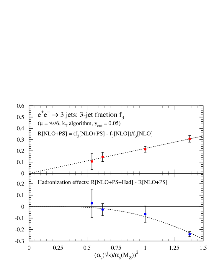
Figure 6: Comparison of the NLO calculation with showers to a pure NLO calculation. In the top panel, we plot the ratio $R[\mbox{\tt NLO+PS}]$ defined in Eq. (6). We take $y_{\rm cut}=0.05$ and $\mu=\sqrt{s}/6$. The ratio $R$ is calculated for the c.m. energies $\sqrt{s}=34$ GeV, $M_{Z}$, 500 GeV and 1000 GeV, corresponding to $\alpha_{s}=0.139$, 0.118, 0.0940 and 0.0868, respectively, and is plotted versus $\alpha_{s}^{2}(\sqrt{s})/\alpha_{s}^{2}(M_{Z})$. For comparison, the curve $R=0.22\,\alpha_{s}^{2}(\sqrt{s})/\alpha_{s}^{2}(M_{Z})$ is shown. In the bottom panel, we show the difference between $R$ calculated with hadronization and $R$ calculated without hadronization. For comparison, we show the curve $\Delta R=8\ {\rm GeV}/\sqrt{s}$.

A next-to-leading order calculation is supposed to do better than a leading order calculation because of its reduced uncertainty from uncalculated terms in the perturbative expansion. Some of the uncalculated terms contain logarithms of the renormalization scale. Thus one way to crudely estimate this uncertainty is to vary the renormalization scale by, say, a factor of two and see how the calculated quantity responds. In Fig. 7, we try this for $f_{3}[\mbox{\tt NLO+PS+Had}]$ at $y_{\rm cut}=0.05$. We vary the renormalization scale $\mu$ in the perturbative part of the calculation while keeping the Pythia parameters unchanged. We see that $f_{3}[\mbox{\tt NLO+PS+Had}]$ changes by about 5% when we increase or decrease $\mu$ by a factor 2. This is quite a small change that, we suspect, underestimates the uncertainty, since the difference between $f_{3}[\mbox{\tt NLO+PS+Had}]$ and $f_{3}[\mbox{\tt NLO}]$ is 10% . The $\mu$ dependence of the NLO calculation is even smaller. By way of comparison, we vary by a factor 2 the parameter in Pythia that controls the scale (PARJ(81)). As shown in Fig. 7, the result changes by about 15%, consistent with the scale variation of the pure LO result.

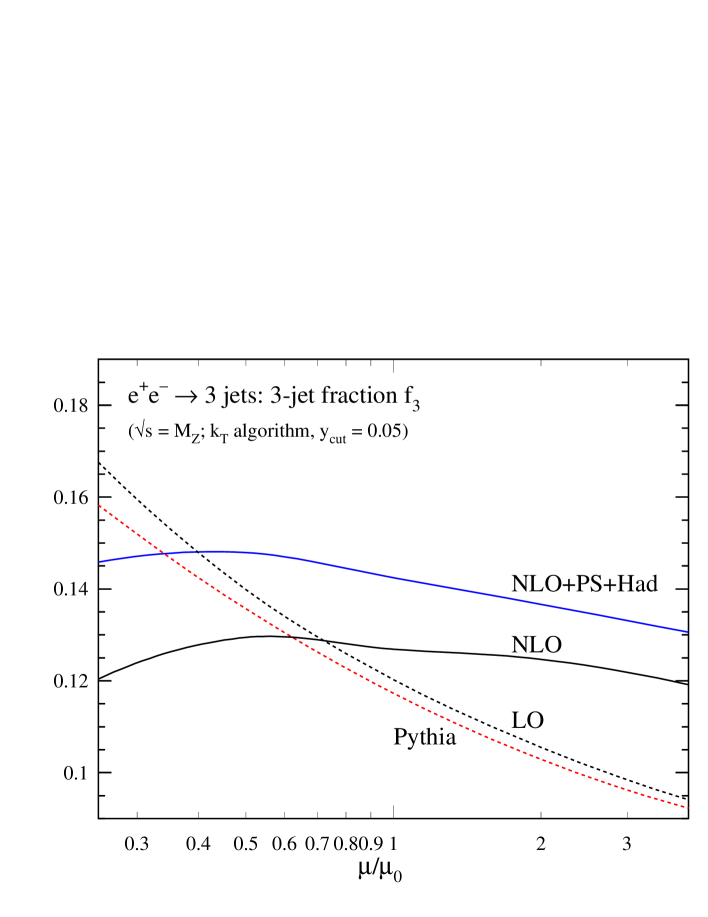
Figure 7: Three-jet fraction, $f_{3}$ versus $\mu/\mu_{0}$, where $\mu$ is the renormalization scale and $\mu_{0}$ is its default value. We show the result of the full NLO+PS+Had calculation and for the pure NLO calculation. In these calculations the default scale is $\mu_{0}=\sqrt{s}/6$. For comparison, we also show the result of varying the scale in plain Pythia. In this case, the default value, $\mu_{0}$ of the scale $\mu$ in $\alpha_{s}(\mu)$ is the transverse momentum in the parton splitting. The ratio $\mu/\mu_{0}$ is the inverse of the Pythia parameter PARJ(81). We choose default parameters as in Fig. 1.

Now we turn to the distribution of jet masses in three jet events, $f_{3}^{-1}\,df_{3}/dM$. We recall from Fig. 1 that $f_{3}^{-1}\,df_{3}[{\tt NLO}]/dM$ is completely unrealistic in the small mass region. In Fig. 9, we plot $f_{3}^{-1}\,df_{3}[\mbox{\tt NLO+PS+Had}]/dM$ versus $M$. Both the unbounded increase in the cross section as $M\to 0$ and the large negative contribution at $M=0$ are gone. In fact, the distribution looks a lot like the distribution produced by Pythia, Fig. 2, as can be seen from the direct comparison between $f_{3}^{-1}\,df_{3}[\mbox{\tt NLO+PS+Had}]/dM$ and $f_{3}^{-1}\,df_{3}[{\tt Pythia}]/dM$ in Fig. 9. It is worthy of notice in Fig. 9 that Pythia gets a result for $f_{3}^{-1}\,df_{3}/dM$ that is in good agreement with $df_{3}[\mbox{\tt NLO+PS+Had}]/dM$ without using next-to-leading order corrections.

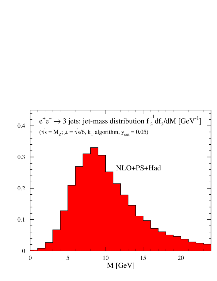
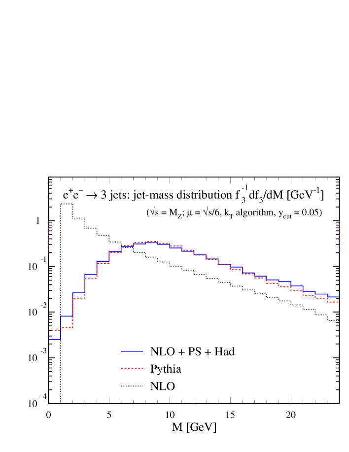
Figure 8: Distribution of jet masses in three jet events, $f_{3}^{-1}\,df_{3}/dM$, in the full NLO+PS+Had calculation using $y_{\rm cut}=0.05$. The result is substantially changed from Fig. 1 and is much closer to the result in Fig. 2. The calculation is defined as in Fig. 1.

Figure 9: Distribution of jet masses in three jet events, $f_{3}^{-1}\,df_{3}/dM$, in the full NLO+PS+Had calculation, in the Pythia calculation and in the pure NLO calculation. The calculations are defined as in Figs. 1 and 2. The NLO distribution is negative in the first mass bin, although this is not visible in a semilog plot.

Finally, in Fig. 10 we investigate the effect of hadronization by comparing $f_{3}^{-1}\,df_{3}[\mbox{\tt NLO+PS+Had}]/dM$ to the same quantity with hadronization turned off, $df_{3}[\mbox{\tt NLO+PS}]/dM$. We see that without hadronization, both the unbounded increase in the NLO cross section as $M\to 0$ and the large negative contribution at $M=0$ are gone. However, there is still a substantial probability to produce a jet with very small mass. With hadronization, it is no longer probable to produce a jet with mass less than 5 GeV. On the other hand, some 2 GeV is added to the mass of typical large mass jets, thus boosting the cross section at any fixed value of the jet mass above about 5 GeV. This effect explains most of the difference between $f_{3}^{-1}\,df_{3}[\mbox{\tt NLO+PS+Had}]/dM$ and $f_{3}^{-1}\,df_{3}[\mbox{\tt NLO}]/dM$ at large jet masses.

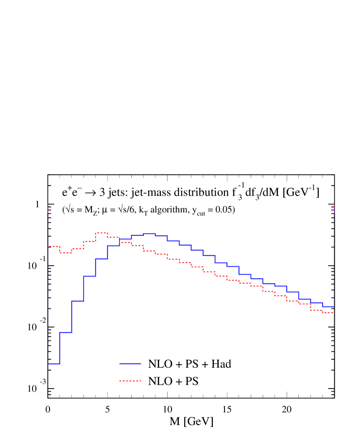
Figure 10: Comparison of $f_{3}^{-1}\,df_{3}[\mbox{\tt NLO+PS+Had}]/dM$ to the same quantity not including hadronization, $f_{3}^{-1}\,df_{3}[\mbox{\tt NLO+PS}]/dM$. Hadronization increases the masses of jets. The calculation is defined as in Fig. 1.

V Parameter dependence

The algorithm for combining an NLO calculation with showers described in Refs. nloshowersI ; nloshowersII incorporates some adjustable parameters, most notably the two denoted as $\lambda_{V}$ and $\lambda_{\rm soft}$. The calculated value of an observable like the three-jet fraction is supposed to be correct to next-to-leading order independent of the choices of values of these parameters. Thus $f_{3}$ should be relatively insensitive $\lambda_{V}$ and $\lambda_{\rm soft}$. In this section we check whether this is so.

We begin with $\lambda_{V}$, which we can treat adequately with just two paragraphs. Consider the splitting of one of the partons from a Born graph, as represented by one of the square vertices in Fig. 3. We call this a primary splitting. In a primary splitting, there is an integration over the virtuality $\bar{q}^{2}$ of the pair of daughter partons. In principle it is possible to use an integration range $0<\bar{q}^{2}<\infty$, since there is an automatic cutoff imposed by the kinematics of the calculation. However, one can impose a cut $\bar{q}^{2}<\lambda_{V}\,\vec{q}^{\,2}$, where $\vec{q}$ is the three-momentum carried by the pair of daughter partons. Taking $\lambda_{V}<\infty$ changes the result from the Born graphs, but there is a compensating adjustment in the order $\alpha_{s}^{B+1}$ terms. One might imagine that taking $\lambda_{V}<\infty$ is worthwhile because the parton splitting approximation with its Sudakov suppression, which is sensible at small virtualities, is then used only at small or moderate virtuality, while we use ordinary fixed order perturbation theory in the large virtuality region. The default value in the program is $\lambda_{V}=1$. We have calculated $f_{3}$ at $y_{\rm cut}=0.05$ and $\sqrt{s}=M_{Z}$ for a range of values of $\lambda_{V}$. We find that taking $\lambda_{V}<0.5$ makes $f_{3}[\mbox{\tt NLO+PS+Had}]$ too big. However, in the range $0.5<\lambda_{V}<\infty$, $f_{3}$ is independent of $\lambda_{V}$ to within 10%. One might simply set $\lambda_{V}\to\infty$, thus eliminating it from the algorithm, except that very large values of $\lambda_{V}$ allow contributions from the region of finite $\bar{q}^{2}$ with $\vec{q}^{\,2}\to 0$. There is a singularity here (an artifact of the use of Coulomb gauge in the Feynman diagrams), producing undesirable fluctuations in the results.

We examine next the parameter denoted as $\lambda_{\rm soft}$ in Refs. nloshowersI ; nloshowersII . Consider the soft gluon emitted from the antenna produced by the three partons emitted in a Born graph, which is represented in Fig. 3 as a gluon emitted from the outgoing partons as a whole. The approximations used for the gluon emission are valid only when the gluon momentum is small. For this reason we impose a limit on the energy of the emitted gluon,

$$E<M_{\rm soft}\equiv\lambda_{\rm soft}\sqrt{s}_{0}\,(1-t_{0})\;,$$ (7)

where $\sqrt{s}_{0}$ is the c.m. energy of the three parton final state at the Born level (before showering) and $t_{0}$ is the thrust value associated with this state. The default value of $\lambda_{\rm soft}$ is 1/3. Changing $\lambda_{\rm soft}$ changes the contribution from the Born graphs, but there is a compensating change in the order $\alpha_{s}^{B+1}$ graphs, so that the net change is of order $\alpha_{s}^{B+2}$.

In Fig. 11 we show how the calculated three-jet fraction depends on $\lambda_{\rm soft}$.

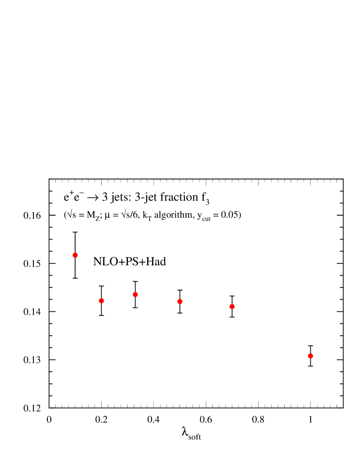
Figure 11: Dependence of $f_{3}[\mbox{\tt NLO+PS+Had}]$ on the soft gluon cutoff parameter $\lambda_{\rm soft}$. The calculation is defined as in Fig. 1.

We see that varying $\lambda_{\rm soft}$ over a substantial range, $0.1<\lambda_{\rm soft}<1$, results in only a 10% change in the answer. We also see that, if we make $\lambda_{\rm soft}$ much smaller than 1/3, the statistical uncertainty in the numerical integration increases. The reason is that in the $\alpha_{s}^{B+1}$ graphs there are subtraction terms that remove the leading soft gluon singularities and the integration range covered by these subtraction is $|\vec{k}|<M_{\rm soft}$. Effectively this inserts a cutoff $|\vec{k}|>M_{\rm soft}$ in the integrations over gluon momenta in the $\alpha_{s}^{B+1}$ graphs. With a very small value of $\lambda_{\rm soft}$, the cutoff is removed. Then real emission graphs cancel virtual loop graphs after integration, but we encounter large positive and negative values point by point in the integration.

There is another approach that one might have taken. One might leave the subtraction terms in the order $\alpha_{s}^{B+1}$ graphs but simply omit the soft gluon emission from the Born graphs. This is not valid at next-to-leading order when $\lambda_{\rm soft}$ is finite, but it is allowed if $\lambda_{\rm soft}$ is small enough. The reason is that the soft gluon emission from the Born graphs does not affect the measurement function as long as the gluon momentum is very small and the measurement function is infrared safe. Thus leaving out the soft gluon emission from the Born graphs is allowed if we check the dependence of the calculated quantity on $\lambda_{\rm soft}$ in order to see how small is “small enough.” This is similar to the procedure adopted in Refs. FrixioneWebberI ; FrixioneWebberII ; FrixioneWebberIII , where the corresponding cutoff parameter is called $\beta$. We have tried this for the three-jet fraction and show the results in Fig. 12. What we find is that even $\lambda_{\rm soft}=1$ is “small enough.” That is, we need the subtraction terms, or some other soft gluon cutoff, in the $\alpha_{s}^{B+1}$ graphs in order for the numerical integrations to work, but the three-jet fraction is so insensitive to soft gluons that one could do without the soft gluon emission that compensates for the net effect of the subtraction terms. This finding helps to justify the approach in Refs. FrixioneWebberI ; FrixioneWebberII ; FrixioneWebberIII .

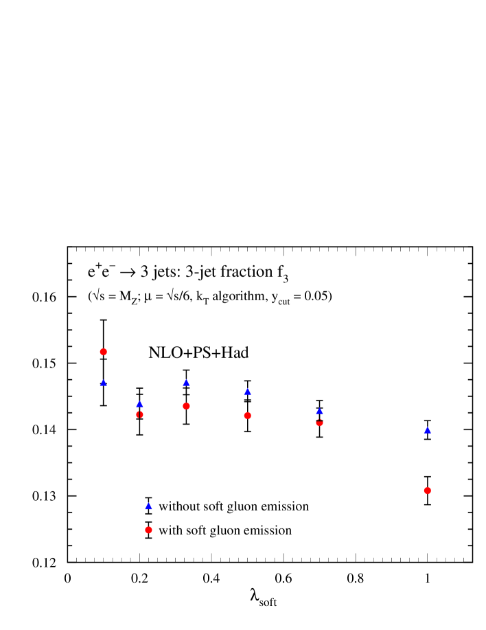
Figure 12: Dependence of $f_{3}$ on the soft gluon cutoff parameter $\lambda_{\rm soft}$ if the soft gluon emission from Born graphs is omitted. Also shown is $f_{3}[\mbox{\tt NLO+PS+Had}]$ from Fig. 11. The calculation is defined as in Fig. 1.

VI Conclusions

We have presented results from a method for adding parton showers to next-to-leading order calculations in QCD when the Born process involves massless strongly interacting partons. Specifically, the process investigated is $e^{+}e^{-}\to 3\ {\it jets}$. We start with an algorithm nloshowersI ; nloshowersII for coupling the NLO calculation to the first, hardest step in showering. Here the problem is to include the parton splittings that are part of the NLO calculation and the parton splittings that are part of the first step of showering without double counting. For our numerical results we have matched the NLO calculation to the standard Monte Carlo event generator Pythia, although the method is more general and there is no limitation in principle to using another event generator. We have arranged for Pythia to be able to accept the partly developed shower and perform the rest of the showering plus hadronization. With an NLO program working together with Pythia, one can accomplish two things at once: calculate infrared-safe three jet quantities like the three jet fraction $f_{3}$ with the reduced theoretical error characteristic of a NLO calculation and get a sensible description of the inner structure of the three jets.

Future NLO-MC hybrid programs will likely be more sophisticated than this one and less tied to a particular Monte Carlo program than that of Ref. FrixioneWebberI ; FrixioneWebberII ; FrixioneWebberIII . They may employ the refined and simplified version of the matching algorithm presented in Ref. Nagy:2005aa . This newer algorithm is based on a commonly used subtraction formalism for performing NLO calculations, and it provides more flexibility by allowing to switch from a three-jet description to a two-jet description for events that are close to a two-jet configuration.

- (1) Y.L. Dokshitzer, in Workshop on jet studies at LEP and HERA, Durham, 1990, reported in W. J. Stirling, J. Phys. G 17 (1991) 1567; S. Catani, Y. L. Dokshitzer, M. Olsson, G. Turnock and B. R. Webber, Phys. Lett. B 269 (1991) 432; see also S. Bethke, Z. Kunszt, D. E. Soper and W. J. Stirling, Nucl. Phys. B 370 (1992) 310 [Erratum-ibid. B 523 (1998) 681].
- (2) T. Sjöstrand, Comput. Phys. Commun. 39 (1986) 347; T. Sjöstrand, P. Eden, C. Friberg, L. Lönnblad, G. Miu, S. Mrenna and E. Norrbin, Comput. Phys. Commun. 135, 238 (2001) [arXiv:hep-ph/0010017].
- (3) G. Marchesini, B. R. Webber, G. Abbiendi, I. G. Knowles, M. H. Seymour and L. Stanco, Comput. Phys. Commun. 67, 465 (1992); G. Corcella et al., JHEP 0101 010 (2001) [arXiv:hep-ph/0011363].
- (4) L. Lönnblad, Comput. Phys. Commun. 71, 15 (1992).
- (5) D. E. Soper, Phys. Rev. Lett. 81, 2638 (1998) [arXiv:hep-ph/9804454]; Phys. Rev. D 62, 014009 (2000) [arXiv:hep-ph/9910292]; Phys. Rev. D 64, 034018 (2001) [arXiv:hep-ph/0103262]; M. Krämer and D. E. Soper, Phys. Rev. D 66 (2002) 054017 [arXiv:hep-ph/0204113].
- (6) S. Frixione and B. R. Webber, JHEP 0206, 029 (2002) [arXiv:hep-ph/0204244].
- (7) S. Frixione, P. Nason and B. R. Webber, JHEP 0308, 007 (2003) [arXiv:hep-ph/0305252].
- (8) S. Frixione and B. R. Webber, arXiv:hep-ph/0402116.
- (9) P. Nason, JHEP 0411 (2004) 040 [arXiv:hep-ph/0409146].
- (10) M. Krämer and D. E. Soper, Phys. Rev. D 69, 054019 (2004) [arXiv:hep-ph/0306222].
- (11) D. E. Soper, Phys. Rev. D 69, 054020 (2004) [arXiv:hep-ph/0306268].
- (12) D. E. Soper, beowulf website, http://physics.uoregon.edu/∼soper/beowulf/.
- (13) S. Mrenna, [arXiv:hep-ph/9902471]; B. Pötter, Phys. Rev. D 63, 114017 (2001) [arXiv:hep-ph/0007172]; M. Dobbs, Phys. Rev. D 64, 034016 (2001) [arXiv:hep-ph/0103174]; B. Pötter and T. Schörner, Phys. Lett. B 517, 86 (2001) [arXiv:hep-ph/0104261]; M. Dobbs, Phys. Rev. D 65, 094011 (2002) [arXiv:hep-ph/0111234]; Y. Kurihara, J. Fujimoto, T. Ishikawa, K. Kato, S. Kawabata, T. Munehisa and H. Tanaka, Nucl. Phys. B 654 (2003) 301 [arXiv:hep-ph/0212216]; J. C. Collins, JHEP 0005, 004 (2000) [arXiv:hep-ph/0001040]; J. C. Collins and F. Hautmann, JHEP 0103, 016 (2001) [arXiv:hep-ph/0009286]; Y. Chen, J. C. Collins and N. Tkachuk, JHEP 0106, 015 (2001) [arXiv:hep-ph/0105291]; J. C. Collins and X. Zu, JHEP 0206, 018 (2002) [arXiv:hep-ph/0204127].
- (14) S. Catani, F. Krauss, R. Kuhn and B. R. Webber, JHEP 0111, 063 (2001) [arXiv:hep-ph/0109231].
- (15) S. Mrenna and P. Richardson, JHEP 0405, 040 (2004) [arXiv:hep-ph/0312274].
- (16) Z. Nagy and D. E. Soper, arXiv:hep-ph/0503053.
- (17) E. Boos et al., arXiv:hep-ph/0109068.