Fermion self-energies and pole masses at two-loop order in a general renormalizable theory with massless gauge bosons

Abstract

I present the two-loop self-energy functions and pole masses for fermions in an arbitrary renormalizable field theory, in the approximation that vector bosons are treated as massless. The calculations are done simultaneously in the mass-independent $\overline{\rm MS}$, $\overline{\rm DR}$, and $\overline{\rm DR}^{\prime}$ renormalization schemes, with a general covariant gauge fixing, and treating Majorana and Dirac fermions in a unified way. As examples, I discuss the two-loop strong interaction corrections to the gluino, neutralino, chargino, and quark pole masses in minimal supersymmetry. All other two-loop contributions to the fermion pole masses in softly-broken supersymmetry can also be obtained as special cases of the results given here, neglecting only the electroweak symmetry breaking scale compared to larger mass scales in two-loop diagrams that involve $W$ or $Z$ bosons.

I Introduction

The CERN Large Hadron Collider and a future electron-positron linear collider should discover and, together, thoroughly explore LHCILC the mechanism behind electroweak symmetry breaking. The small ratio of the scale of electroweak symmetry breaking to the Planck mass scale suggests that supersymmetric particles will also be found at these next-generation experiments. If so, then a primary goal of both experimental and theoretical research will be to unravel the mechanism behind supersymmetry breaking. The most important clues will be the masses of the superpartners and the Higgs scalar bosons. Therefore it is important to be able to compute the physical masses accurately in terms of the underlying Lagrangian parameters, including at least the leading two-loop effects.

In this paper, I will present results for the two-loop contributions to fermion self-energy functions and physical pole masses in a general renormalizable field theory, in terms of the running renormalized couplings and masses. The approach used is intended to be as flexible as possible, so that a common framework of calculation can be used to treat both Majorana and Dirac fermions, including chiral interactions, in both supersymmetric and non-supersymmetric theories. As a simplifying approximation, vector bosons will be treated as massless in the two-loop parts in this paper. In the Standard Model and extensions of it that do not enlarge the gauge group, this amounts to neglecting the effects of electroweak symmetry breaking compared to the masses of heavier particles in two-loop diagrams that have $W$ and/or $Z$ boson propagators. (The effects of non-zero $W$ and $Z$ boson masses can be included as usual in the one-loop part.) This will likely be a good approximation for the pole masses of the top quark and most of the supersymmetric particles, because of the exclusions of light squarks, sleptons, and gluinos already achieved by the CERN LEP $e^{+}e^{-}$ collider LEPSUSY and the Fermilab Tevatron $p\overline{p}$ collider squarksDzero ; squarksCDF .

The mass defined by the position of the complex pole in the propagator is a gauge-invariant and renormalization scale-invariant quantity Tarrach:1980up -Gambino:1999ai . The pole mass in principle does suffer from ambiguities poleambiguities due to infrared physics associated with the QCD confinement scale, but these are probably relatively too small to cause a practical problem for strongly-interacting superpartners. The pole mass should be closely related in a calculable way to the kinematic observable mass reported by experiments massdefs . In recent years, many important higher-order calculations of self-energy functions and pole masses in the Standard Model have been performed, including two-loop Gray:1990yh -Jegerlehner:2003py and three-loop Chetyrkin:1999qi -Melnikov:2000qh contributions for quarks, and two-loop results for electroweak vector bosons Chang:1981qq -Jegerlehner:2001fb . In addition, there are important two-loop results for top and bottom quarks quarkpoleSUSYa ; quarkpoleSUSYb ; Bednyakov:2005kt and the gluino Yamada:2005ua in low-energy supersymmetry. The general treatment of the present paper will confirm and extend the results of those papers.

The notation and strategy used here are very similar to those found in my previous papers on scalar self-energy functions and pole masses at two-loop order in a general theory Martin:2003it ; Martin:2005eg . In the next section, I review the conventions used, discuss the formalism for self-energy functions and pole masses for fermions in a two-component notation, and review the methods used for numerical evaluation of the required two-loop integrals.

II Notations and setup

II.1 Notations for fields, interactions, and indices

In this paper, the spacetime metric tensor is

$$\eta^{\mu\nu}=\mbox{diag}(-1,+1,+1,+1).$$ (2.1)

I use a two-component notation for fermions, as in ref. Martin:1997ns and similar to that found in ref. WessBaggerbook . Left-handed spinor fields $\psi_{\alpha}$ always carry undotted spinor indices $\alpha,\beta,\ldots=1,2$, and right-handed spinor fields $\psi^{\dagger}_{\dot{\alpha}}$ always carry daggers and dotted spinor indices $\dot{\alpha},\dot{\beta},\ldots=1,2$, with

$$\psi^{\dagger}_{\dot{\alpha}}\equiv(\psi_{\alpha})^{\dagger}.$$ (2.2)

However, the spinor indices are most often suppressed, as described below. The spinor indices are raised and lowered with the two-index antisymmetric symbol with components $\epsilon^{12}=-\epsilon^{21}=\epsilon_{21}=-\epsilon_{12}=1$, and the same set of sign conventions for the corresponding dotted spinor indices. Thus

$$\psi_{\alpha}=\epsilon_{\alpha\beta}\psi^{\beta}\,,\qquad\psi^{\alpha}=\epsilon^{\alpha\beta}\psi_{\beta}\,,$$ (2.3)

$$\psi^{\dagger}_{\dot{\alpha}}=\epsilon_{\dot{\alpha}\dot{\beta}}\psi^{\dagger\dot{\beta}}\,,\qquad\psi^{\dagger\dot{\alpha}}=\epsilon^{\dot{\alpha}\dot{\beta}}\psi^{\dagger}_{\dot{\beta}}\,.$$ (2.4)

Spinor bilinears can be combined to form vector quantities using the matrices $\sigma_{\mu\,\alpha{\dot{\beta}}}$ and $\overline{\sigma}_{\mu}^{\dot{\alpha}\beta}$ defined by

$$\!\!\!\!\!\!\!\!\!\!\overline{\sigma}_{0}=\sigma_{0}=\begin{pmatrix}1&0\\ 0&1\end{pmatrix},\qquad\overline{\sigma}_{1}=-\sigma_{1}=\begin{pmatrix}0&1\\ 1&0\end{pmatrix},$$

$$\!\!\!\!\!\!\!\!\!\!\overline{\sigma}_{2}=-\sigma_{2}=\begin{pmatrix}0&-i\\ i&0\end{pmatrix},\quad\overline{\sigma}_{3}=-\sigma_{3}=\begin{pmatrix}1&0\\ 0&-1\end{pmatrix}.\phantom{x}$$ (2.5)

When constructing Lorentz tensors from fermion fields, the heights of spinor indices must be consistent in the sense that lowered indices must only be contracted with raised indices. As a convention, indices contracted like ${}^{\alpha}{}_{\alpha}$ and ${}_{\dot{\alpha}}{}^{\dot{\alpha}},$ can be suppressed. For example,

$$\xi\chi \equiv \xi^{\alpha}\chi_{\alpha},$$ (2.6)

$$\xi^{\dagger}\chi^{\dagger} \equiv \xi^{\dagger}_{\dot{\alpha}}\chi^{\dagger\dot{\alpha}},$$ (2.7)

$$\xi^{\dagger}\overline{\sigma}^{\mu}\chi \equiv \xi^{\dagger}_{\dot{\alpha}}\overline{\sigma}^{\mu\dot{\alpha}\beta}\chi_{\beta},$$ (2.8)

$$\xi\sigma^{\mu}\chi^{\dagger} \equiv \xi^{{\alpha}}\sigma^{\mu}_{\alpha\dot{\beta}}\chi^{\dagger\dot{\beta}}.$$ (2.9)

The behavior of the spinor products under hermitian conjugation (for quantum field operators) or complex conjugation (for classical fields) is as follows:

$$(\xi\chi)^{\dagger}=\chi^{\dagger}\xi^{\dagger},$$ (2.10)

$$(\xi\sigma^{\mu}\chi^{\dagger})^{\dagger}=\chi\sigma^{\mu}\xi^{\dagger},$$ (2.11)

$$(\xi^{\dagger}\overline{\sigma}^{\mu}\chi)^{\dagger}=\chi^{\dagger}\overline{\sigma}^{\mu}\xi.$$ (2.12)

The following identities also hold:

$${[\sigma^{\mu}\overline{\sigma}^{\nu}+\sigma^{\nu}\overline{\sigma}^{\mu}]_{\alpha}}^{\beta}=-2\eta^{\mu\nu}\delta_{\alpha}^{\beta},$$ (2.13)

$$[\overline{\sigma}^{\mu}\sigma^{\nu}+\overline{\sigma}^{\nu}\sigma^{\mu}]^{\dot{\alpha}}{}_{\dot{\beta}}=-2\eta^{\mu\nu}\delta^{\dot{\alpha}}_{\dot{\beta}},$$ (2.14)

$${\rm Tr}[\sigma^{\mu}\overline{\sigma}^{\nu}]={\rm Tr}[\overline{\sigma}^{\mu}\sigma^{\nu}]=-2\eta^{\mu\nu}.$$ (2.15)

In terms of two-component fermion notation, a single Dirac fermion is given in the chiral representation by

$$\Psi=\begin{pmatrix}\xi_{\alpha}\\ \chi^{\dagger\dot{\alpha}}\end{pmatrix},$$ (2.16)

where $\xi$ is the two-component fermion that describes the left-handed part of $\Psi$ and $\chi$ is the two-component fermion that describes the conjugate of the right-handed part of $\Psi$. The Dirac matrices are

$$\gamma_{\mu}=\begin{pmatrix}0&\sigma_{\mu}\\ \overline{\sigma}_{\mu}&0\end{pmatrix}.$$ (2.17)

In this paper, I consider a general renormalizable field theory, containing a set of real scalars $R_{i}$, two-component Weyl fermions $\psi_{I}$, and vector bosons $V^{\mu}_{a}$. Scalar field indices are $i,j,k,\ldots$, fermion flavor indices are $I,J,K,\ldots$, and $a,b,c,\ldots$ run over the adjoint representation of the gauge group, while $\mu,\nu,\ldots$ are space-time vector indices. Repeated indices of all types are summed over unless otherwise noted.

The masses and couplings are evaluated by taking the fields in the Lagrangian in a squared-mass eigenstate basis, after the Higgs fields are assumed to have been expanded around their vacuum expectation values as determined by the loop-corrected effective potential (so that tadpole graphs do not contribute). The kinetic part of the renormalized tree-level Lagrangian is then written as:

$${\cal L}_{\rm kin} = -\frac{1}{2}\partial_{\mu}R_{i}\partial^{\mu}R_{i}-\frac{1}{2}m^{2}_{i}R_{i}^{2}$$ (2.18)

$$-i\psi^{\dagger I}\overline{\sigma}^{\mu}\partial_{\mu}\psi_{I}-\frac{1}{2}(m^{IJ}\psi_{I}\psi_{J}+{\rm c.c.})$$

$$-\frac{1}{2}(\partial_{\mu}V_{\nu}^{a}-\partial_{\nu}V_{\mu}^{a})\partial^{\mu}V^{\nu}_{a}-\frac{1}{2}m^{2}_{a}V_{\mu}^{a}V^{\mu}_{a}.\phantom{xxx}$$

The non-gauge interactions of the scalar and fermion fields are given by the renormalized Lagrangian:

$${\cal L}_{\rm int} = -\frac{1}{6}\lambda^{ijk}R_{i}R_{j}R_{k}-\frac{1}{24}\lambda^{ijkm}R_{i}R_{j}R_{k}R_{m}$$ (2.19)

$$-\frac{1}{2}(y^{JKi}\psi_{J}\psi_{K}R_{i}+{\rm c.c.}).$$

where $\lambda^{ijk}$ and $\lambda^{ijkm}$ are real couplings and the Yukawa couplings $y^{JKi}$ are symmetric complex matrices on the indices $J,K$, for each $i$. Raising or lowering of fermion indices implies complex conjugation of the Lagrangian parameters, so

$$m_{IJ}\equiv(m^{IJ})^{*},\qquad y_{JKi}\equiv(y^{JKi})^{*}.$$ (2.20)

Actually, without loss of generality, $m^{IJ}$ can be taken to have only real and non-negative entries, but the index height convention is maintained for clarity. The heights of real scalar and vector indices have no significance, and in any given equation are chosen for convenience.

The scalar squared masses $m_{i}^{2}$ and the fermion squared masses $m_{IK}m^{KJ}=m^{2}_{I}\delta_{I}^{J}$ are taken to have been diagonalized (by an appropriate rotation of the fields if necessary). However, the fermion mass matrix $m^{IJ}$ is not necessarily diagonal; instead it must have non-zero entries only when $I$ and $J$ label two-component fermions with the same squared mass and in conjugate representations of the unbroken gauge group. In particular, when dealing with Dirac fermions, it is most useful to work in a basis in which the corresponding matrix $m^{IJ}$ contains $2\times 2$ blocks of the form $\begin{pmatrix}0&m\cr m&0\end{pmatrix}$ on the diagonal.

Next consider the gauge interactions of the theory. Let $T^{a}$ be the Hermitian generator matrices of the gauge group for a (possibly reducible) representation $R$. They are labeled by an adjoint representation index $a$ corresponding to the vector bosons of the theory, $V_{a}^{\mu}$. They satisfy $[T^{a},T^{b}]=if^{abc}T^{c}$, where $f^{abc}$ are the totally antisymmetric structure constants of the gauge group. Then results below are written in terms of the invariants:

$${(T^{a}T^{a})_{i}}^{j} = C(i)\delta_{i}^{j},$$ (2.21)

$${\rm Tr}[T^{a}T^{b}] = I(R)\delta^{ab},$$ (2.22)

$$f^{acd}f^{bcd} = C(G)\delta^{ab},$$ (2.23)

which define the quadratic Casimir invariant for the representation carrying the index $i$, the total Dynkin index summed over the representation $R$, and the Casimir invariant of the adjoint representation of the group, respectively. When the gauge group contains several simple or $U(1)$ factors with distinct gauge couplings $g_{a}$, the corresponding invariants are written $C_{a}(i)$, $I_{a}(R)$, and $C_{a}(G)$. The normalization is such that for $SU(N)$, $C(G)=N$ and each fundamental representation has $C(i)=(N^{2}-1)/2N$ and contributes $1/2$ to $I(R)$ for each Weyl fermion or complex scalar. For a $U(1)$ gauge group, $C(G)=0$ and a representation with charge $q$ has $C(i)=q^{2}$ and contributes $q^{2}$ to $I(R)$. The two-loop results given below will be presented in terms of these group theory invariants for the representations carried by the scalar and fermion degrees of freedom.

The preceding paragraph applies to the two-loop parts, in which the gauge group is treated as unbroken and $m_{a}^{2}=0$. In the one-loop parts of the self-energy functions and the fermion pole masses, the effects of non-zero vector boson masses will be retained. This means that the gauge group cannot be treated as unbroken, and the interactions of the vector bosons with the fermions have a more general form. They can be written as:

$${\cal L}_{\rm gauge}=-g^{aJ}_{I}V_{\mu}^{a}\psi^{\dagger I}\overline{\sigma}^{\mu}\psi_{J}$$ (2.24)

where $g^{aJ}_{I}$ are couplings obtained by going to the tree-level mass eigenstate basis for the fermions and vector bosons. In the special case of an unbroken gauge symmetry, one has $g^{aJ}_{I}=g_{a}[T^{a}]_{I}{}^{J}$.

The computations in this paper are performed with a vector boson propagator obtained by covariant gauge fixing in the usual way:

$$-i\delta_{ab}\bigl{(}\eta^{\mu\nu}+k^{\mu}k^{\nu}{\cal L}_{m_{a}^{2}}\bigr{)}\left[1/(k^{2}+m_{a}^{2})\right],\phantom{xx}$$ (2.25)

where for later convenience I use the notation

$${\cal L}_{x}f(x)\equiv[f(x)-f(\xi x)]/x,$$ (2.26)

with the appropriate limit for massless vectors:

$$\lim_{x\rightarrow 0}\left[{\cal L}_{x}f(x)\right]=(1-\xi)f^{\prime}(0).$$ (2.27)

Here $\xi=0,1,$ and $3$ correspond to the Landau, Feynman, and Fried-Yennie gauge-fixing choices, respectively. The self-energy functions depend on $\xi$, but the pole masses do not. For the two-loop computations below, the vector bosons are treated as massless, so the propagators are

$$-i\delta_{ab}[\eta^{\mu\nu}/k^{2}-(1-\xi)k^{\mu}k^{\nu}/(k^{2})^{2}].$$ (2.28)

Infrared divergences are dealt with by first computing with a finite vector boson mass, and later taking the massless vector limit. All contributions involving gauge boson loops implicitly include the corresponding contributions of ghost loops.

II.2 Regularization and renormalization

For each Feynman diagram, the integrations over internal momenta are regulated by continuing to $d=4-2\epsilon$ dimensions, according to

$$\int d^{4}k\rightarrow(2\pi\mu)^{2\epsilon}\int d^{d}k.$$ (2.29)

In the dimensional regularization scheme, the vector bosons also have $d$ components, while in the dimensional reduction scheme they have $d$ ordinary components and $2\epsilon$ additional components known as epsilon scalars. This means that the 4-dimensional metric in the vector propagator of eq. (2.25) is replaced by

$$\eta^{\mu\nu}/(k^{2}+m_{a}^{2}) \rightarrow g^{\mu\nu}/(k^{2}+m_{a}^{2})$$ (2.30)

$$+\hat{g}^{\mu\nu}/(k^{2}+m_{a}^{2}+m_{\epsilon}^{2}),$$

where $g^{\mu\nu}$ is projected onto a formal $d$–dimensional subspace, and $\hat{g}^{\mu\nu}$ onto the complementary $2\epsilon$–dimensional subspace, and $m_{\epsilon}^{2}$ is the epsilon scalar squared mass parameter. (In general, there should be a different $m_{\epsilon}^{2}$ for each $a$, but it should cause no confusion to omit the additional subscript in this paper.) Counterterms for the one-loop sub-divergences and the remaining two-loop divergences are added, according to the rules of minimal subtraction, to give finite results, which then depend on the renormalization scale $Q$ given by

$$Q^{2}=4\pi e^{-\gamma}\mu^{2}.$$ (2.31)

Logarithms of dimensionful quantities are always written in terms of

$${\overline{\rm ln}}X\equiv\ln(X/Q^{2}).$$ (2.32)

The resulting renormalization schemes are known as $\overline{\rm MS}$ MSbar and $\overline{\rm DR}$ DRbar , respectively, for the cases in which $\hat{g}^{\mu\nu}$ is not and is included.

The epsilon-scalar squared mass parameter $m_{\epsilon}^{2}$ appearing in the $\overline{\rm DR}$ scheme is unphysical. One could set $m_{\epsilon}^{2}$ equal to zero at any fixed renormalization scale, but then it will be non-zero at other renormalization scales, since it has a non-homogeneous beta function Jack:1994kd . Furthermore, under renormalization group evolution it will feed into the ordinary scalar squared masses in the $\overline{\rm DR}$ scheme. Fortunately, a redefinition (given in DRbarprime at one-loop order, and at two-loop order in effpot ) of the ordinary scalar squared masses completely removes the dependence on the unphysical epsilon scalar squared mass $m_{\epsilon}^{2}$ from the renormalization group equations and the equations relating tree-level parameters to physical observables in softly-broken supersymmetric theories. The resulting $\overline{\rm DR}^{\prime}$ scheme DRbarprime is therefore an appropriate one for realistic models based on supersymmetry, such as the Minimal Supersymmetric Standard Model (MSSM). In this paper, calculations will be presented simultaneously in all three schemes, using the following two notational devices. First,

$$\delta_{\overline{\rm MS}}\equiv\begin{cases}1&\text{for}\quad\overline{\rm MS}\\ 0&\text{for}\quad\overline{\rm DR},\>\overline{\rm DR}^{\prime}.\end{cases}$$ (2.33)

Second, terms that involve the unphysical parameter $m_{\epsilon}^{2}$ should be construed below to apply only to the $\overline{\rm DR}$ scheme, not the $\overline{\rm DR}^{\prime}$ or $\overline{\rm MS}$ schemes.

II.3 Self-energy functions and pole masses for fermions using two-component notation

The full, loop-corrected Feynman propagators with four-momentum $p^{\mu}$ are denoted as shown in Fig. 1, which defines $C_{I}^{J}$, $D^{IJ}$, and $D_{IJ}$ as functions of the masses and couplings of the theory and of the external momentum invariant

$$s\equiv-p^{2}.$$ (2.34)

They are given, starting from tree level, as

$$D^{IJ} = {m}^{IJ}/(p^{2}+m_{I}^{2})+\mbox{\ldots}$$ (2.35)

$$D_{IJ} = {m}_{IJ}/(p^{2}+m_{I}^{2})+\mbox{\ldots}$$ (2.36)

$$C^{J}_{I} = \delta^{J}_{I}/(p^{2}+m_{I}^{2})+\mbox{\ldots}$$ (2.37)

with no sum on $I$ in each case. In general, ${D}^{IJ}$ is a complex symmetric matrix, and ${D}_{IJ}$ is obtained from it by taking the complex conjugate of all Lagrangian parameters appearing in its calculation, but not taking the complex conjugates of loop integral functions, whose imaginary (absorptive) parts correspond to fermion decay widths to multi-particle intermediate states.

The computation of the full propagators can be organized, as usual in quantum field theory, in terms of one-particle irreducible self-energy functions. These are defined in Fig. 2. (The same remark applies for the relationship between the functions $\Omega^{IJ}$, $\Omega_{IJ}$ as for $D^{IJ}$, $D_{IJ}$.) Then one has the matrix diagrammatic identity shown in fig. 3.

Figure 1: The full loop-corrected propagators for fermions in two-component notation are associated with functions $C_{I}^{J}(s)$, $D^{IJ}(s)$, and $D_{IJ}(s)$, as shown. Here $s=-p^{2}$ is the external momentum invariant. The shaded boxes represent the sum of all connected Feynman diagrams, and the external legs are included.

Figure 2: The self-energies for fermions in two-component notation are associated with functions $\Sigma^{I}_{J}(s)$ (for chirality-preserving propagation), and $\Omega^{IJ}(s)$ and $\Omega_{IJ}(s)$ (for chirality-violating propagation), defined as shown. Here $s=-p^{2}$ is the external momentum invariant. The shaded circles represent the sum of all one-particle irreducible, connected Feynman diagrams, and the external legs are not included.

$$\begin{pmatrix}\mbox{\begin{picture}(35.0,21.0)(0.0,10.5)\SetScale{0.7} \ArrowLine(0,25)(17.5,25) \ArrowLine(32.5,25)(50,25) \GBox(17.5,17.5)(32.5,32.5){0.85} \end{picture}}&\,\,\,\,\mbox{\begin{picture}(35.0,21.0)(0.0,10.5)\SetScale{0.7} \ArrowLine(0,25)(17.5,25) \ArrowLine(50,25)(32.5,25) \GBox(17.5,17.5)(32.5,32.5){0.85} \end{picture}}\\ \mbox{\begin{picture}(35.0,21.0)(0.0,10.5)\SetScale{0.7} \ArrowLine(17.5,25)(0,25) \ArrowLine(32.5,25)(50,25) \GBox(17.5,17.5)(32.5,32.5){0.85} \end{picture}}&\,\,\,\,\mbox{\begin{picture}(35.0,21.0)(0.0,10.5)\SetScale{0.7} \ArrowLine(17.5,25)(0,25) \ArrowLine(50,25)(32.5,25) \GBox(17.5,17.5)(32.5,32.5){0.85} \end{picture}}\end{pmatrix}\> = \>\begin{pmatrix}\mbox{\begin{picture}(17.5,21.0)(0.0,10.5)\SetScale{0.7} \ArrowLine(0,25)(30,25) \end{picture}}&\,\,\,\,\mbox{\begin{picture}(20.0,21.0)(0.0,10.5)\SetScale{0.7} \ArrowLine(0,25)(15,25) \ArrowLine(30,25)(15,25) \end{picture}}\\ \mbox{\begin{picture}(17.5,21.0)(0.0,10.5)\SetScale{0.7} \ArrowLine(15,25)(0,25) \ArrowLine(15,25)(30,25) \end{picture}}&\,\,\,\,\,\mbox{\begin{picture}(20.0,21.0)(0.0,10.5)\SetScale{0.7} \ArrowLine(27,25)(0,25) \end{picture}}\end{pmatrix}\left[\begin{pmatrix}\mbox{\begin{picture}(9.8,21.0)(0.0,0.0)\Text(4.9,10.5)[c]{$\bf 1$} \end{picture}}&\,\,\,\,\mbox{\begin{picture}(9.8,21.0)(0.0,0.0)\Text(4.9,10.5)[c]{$\bf 0$} \end{picture}}\\ \mbox{\begin{picture}(9.8,21.0)(0.0,0.0)\Text(4.9,10.5)[c]{$\bf 0$} \end{picture}}&\,\,\,\,\mbox{\begin{picture}(9.8,21.0)(0.0,0.0)\Text(4.9,10.5)[c]{$\bf 1$} \end{picture}}\end{pmatrix}-\begin{pmatrix}\mbox{\begin{picture}(35.0,21.0)(0.0,10.5)\SetScale{0.7} \ArrowLine(0,25)(17.5,25) \ArrowLine(32.5,25)(50,25) \GCirc(25,25){7.5}{0.85} \end{picture}}&\,\,\,\,\mbox{\begin{picture}(35.0,21.0)(0.0,10.5)\SetScale{0.7} \ArrowLine(0,25)(17.5,25) \ArrowLine(50,25)(32.5,25) \GCirc(25,25){7.5}{0.85} \end{picture}}\\ \mbox{\begin{picture}(35.0,21.0)(0.0,10.5)\SetScale{0.7} \ArrowLine(17.5,25)(0,25) \ArrowLine(32.5,25)(50,25) \GCirc(25,25){7.5}{0.85} \end{picture}}&\,\,\,\,\mbox{\begin{picture}(35.0,21.0)(0.0,10.5)\SetScale{0.7} \ArrowLine(17.5,25)(0,25) \ArrowLine(50,25)(32.5,25) \GCirc(25,25){7.5}{0.85} \end{picture}}\end{pmatrix}\begin{pmatrix}\mbox{\begin{picture}(17.5,21.0)(0.0,10.5)\SetScale{0.7} \ArrowLine(0,25)(30,25) \end{picture}}&\,\,\,\,\mbox{\begin{picture}(20.0,21.0)(0.0,10.5)\SetScale{0.7} \ArrowLine(0,25)(15,25) \ArrowLine(30,25)(15,25) \end{picture}}\\ \mbox{\begin{picture}(17.5,21.0)(0.0,10.5)\SetScale{0.7} \ArrowLine(15,25)(0,25) \ArrowLine(15,25)(30,25) \end{picture}}&\,\,\,\,\mbox{\begin{picture}(20.0,21.0)(0.0,10.5)\SetScale{0.7} \ArrowLine(27.5,25)(0,25) \end{picture}}\end{pmatrix}\right]^{-1}$$

$$\>=\> \,\left[\begin{pmatrix}\mbox{\begin{picture}(17.5,21.0)(0.0,10.5)\SetScale{0.7} \ArrowLine(0,25)(30,25) \end{picture}}&\,\,\,\,\mbox{\begin{picture}(20.0,21.0)(0.0,10.5)\SetScale{0.7} \ArrowLine(0,25)(15,25) \ArrowLine(30,25)(15,25) \end{picture}}\\ \mbox{\begin{picture}(17.5,21.0)(0.0,10.5)\SetScale{0.7} \ArrowLine(15,25)(0,25) \ArrowLine(15,25)(30,25) \end{picture}}&\,\,\,\,\mbox{\begin{picture}(20.0,21.0)(0.0,10.5)\SetScale{0.7} \ArrowLine(28,25)(0,25) \end{picture}}\end{pmatrix}^{-1}-\,\begin{pmatrix}\mbox{\begin{picture}(35.0,21.0)(0.0,10.5)\SetScale{0.7} \ArrowLine(0,25)(17.5,25) \ArrowLine(32.5,25)(50,25) \GCirc(25,25){7.5}{0.85} \end{picture}}&\,\,\,\,\mbox{\begin{picture}(35.0,21.0)(0.0,10.5)\SetScale{0.7} \ArrowLine(0,25)(17.5,25) \ArrowLine(50,25)(32.5,25) \GCirc(25,25){7.5}{0.85} \end{picture}}\\ \mbox{\begin{picture}(35.0,21.0)(0.0,10.5)\SetScale{0.7} \ArrowLine(17.5,25)(0,25) \ArrowLine(32.5,25)(50,25) \GCirc(25,25){7.5}{0.85} \end{picture}}&\,\,\,\,\mbox{\begin{picture}(35.0,21.0)(0.0,10.5)\SetScale{0.7} \ArrowLine(17.5,25)(0,25) \ArrowLine(50,25)(32.5,25) \GCirc(25,25){7.5}{0.85} \end{picture}}\end{pmatrix}\right]^{-1}$$

Figure 3: The diagrammatic version of the fermion self-energy identity in eq. (2.43).

To write this in terms of the self-energy functions, denote $N\times N$ matrices (where $N$ is the number of two-component left-handed fermion degrees of freedom, so that $I,J=1,2,\ldots N$):

$${\bf C}_{I}{}^{J}=({\bf C}^{T})^{J}{}_{I}\equiv C_{I}^{J},$$ (2.38)

$${\bf D}^{IJ}\equiv D^{IJ},\qquad\qquad\quad\overline{\bf D}_{IJ}\equiv D_{IJ},$$ (2.39)

$${\bf\Sigma}_{I}{}^{J}=({\bf\Sigma}^{T})^{J}{}_{I}\equiv\Sigma_{I}^{J},$$ (2.40)

$${\bf\Omega}^{IJ}\equiv\Omega^{IJ},\qquad\qquad\>\overline{\bf\Omega}_{IJ}\equiv\Omega_{IJ},$$ (2.41)

$${\bf m}^{IJ}\equiv m^{IJ},\qquad\qquad\quad\overline{\bf m}_{IJ}\equiv m_{IJ},\phantom{xxxx}$$ (2.42)

Then fig. 3 implies that the propagator functions obey the $4N\times 4N$ matrix equation:

$$\begin{pmatrix}ip\kern 0.59998pt{\cdot}\kern 0.59998pt\overline{\sigma}\,{\bf C}^{T}\phantom{x}&-i{\bf D}\\[4.0pt] -i\overline{{\bf D}}\phantom{x}&ip\kern 0.59998pt{\cdot}\kern 0.59998pt\sigma\,{\bf C}\end{pmatrix} = \begin{pmatrix}ip\kern 0.59998pt{\cdot}\kern 0.59998pt\sigma\,[{\bf 1}-{\bf\Sigma}^{T}/s]\phantom{x}&i[{\bf m}+{\bf\Omega}]\\[4.0pt] i[\overline{\bf m}+\overline{\bf\Omega}]&ip\kern 0.59998pt{\cdot}\kern 0.59998pt\overline{\sigma}\,[{\bf 1}-{\bf\Sigma}/s]\end{pmatrix}^{-1}.$$ (2.43)

The pole mass can be found most easily by considering the rest frame of the fermion, in which the space components of the external momentum $p^{\mu}$ vanish. This reduces the spinor-index dependence to a triviality. It follows from eq. (2.43) that the (complex, if the fermion is unstable) poles of the full propagator are the solutions for $s$ of the non-linear $N\times N$ matrix eigenvalue equation:

$${\rm Det}\bigl{[}s{\bf 1}-({\bf 1}-{{\bf\Sigma}}/{s})^{-1}(\overline{\bf m}+\overline{\bf\Omega})({\bf 1}-{{\bf\Sigma}^{T}}/{s})^{-1}({\bf m}+{\bf\Omega})\bigr{]}=0.$$ (2.44)

This can be solved iteratively by first expanding each of the self-energy functions in a Taylor series in $s$ about the tree-level squared masses $m_{I}^{2}$. Write the one- and two-loop contributions to the self-energy functions as:

$$\Sigma_{I}^{J} = \frac{1}{16\pi^{2}}\Sigma_{I}^{(1)J}+\frac{1}{(16\pi^{2})^{2}}\Sigma_{I}^{(2)J}+\ldots$$ (2.45)

$$\Omega^{IJ} = \frac{1}{16\pi^{2}}\Omega^{(1)IJ}+\frac{1}{(16\pi^{2})^{2}}\Omega^{(2)IJ}+\ldots$$ (2.46)

$$\Omega_{IJ} = \frac{1}{16\pi^{2}}\Omega^{(1)}_{IJ}+\frac{1}{(16\pi^{2})^{2}}\Omega^{(2)}_{IJ}+\ldots$$ (2.47)

where the superscripts $(1)$ and $(2)$ refer to the one- and two-loop contributions respectively. Then define the quantities (with sums on $I^{\prime}$, $J^{\prime}$, $K$, and $K^{\prime}$, but not on $I$ or $J$):

$$\Pi^{(1)J}_{I} = \Sigma^{(1)J}_{I}m_{J}^{2}/s+m_{II^{\prime}}\Sigma^{(1)I^{\prime}}_{J^{\prime}}m^{JJ^{\prime}}/s+m_{II^{\prime}}\Omega^{(1)JI^{\prime}}+\Omega^{(1)}_{IJ^{\prime}}m^{JJ^{\prime}},$$ (2.48)

$$\Pi^{(2)J}_{I} = \Sigma^{(2)J}_{I}m_{J}^{2}/s+m_{II^{\prime}}\Sigma^{(2)I^{\prime}}_{J^{\prime}}m^{JJ^{\prime}}/s+m_{II^{\prime}}\Omega^{(2)JI^{\prime}}+\Omega^{(2)}_{IJ^{\prime}}m^{JJ^{\prime}}$$ (2.49)

$$+\Bigl{\{}\Sigma^{(1)K}_{I}\Sigma^{(1)J}_{K}m_{J}^{2}+m_{II^{\prime}}\Sigma^{(1)I^{\prime}}_{K}\Sigma^{(1)K}_{J^{\prime}}m^{JJ^{\prime}}+\Sigma^{(1)K}_{I}m_{KK^{\prime}}\Sigma^{(1)K^{\prime}}_{J^{\prime}}m^{JJ^{\prime}}\Bigr{\}}/s^{2}+\Omega^{(1)}_{IK}\Omega^{(1)JK}$$

$$+\Bigl{\{}\Sigma^{(1)K}_{I}\Omega^{(1)}_{KJ^{\prime}}m^{JJ^{\prime}}+\Sigma^{(1)K}_{I}m_{KK^{\prime}}\Omega^{(1)JK^{\prime}}+m_{II^{\prime}}\Sigma^{(1)I^{\prime}}_{K}\Omega^{(1)JK}+\Omega^{(1)}_{IK}\Sigma^{(1)K}_{J^{\prime}}m^{JJ^{\prime}}\Bigr{\}}/s,$$

which play a role analogous to the self-energy functions of scalar or vector bosons, with eq. (2.44) taking the form

$${\rm Det}\Bigl{[}s\delta_{I}^{J}-\Bigl{(}m_{I}^{2}\delta_{I}^{J}+\frac{1}{16\pi^{2}}\Pi^{(1)J}_{I}+\frac{1}{(16\pi^{2})^{2}}\Pi^{(2)J}_{I}\Bigr{)}\Bigr{]}=0.$$ (2.50)

It follows that the pole squared masses for the fermions are given by (with no sum on the index $I$):

$$s_{{\rm pole},I}\equiv M_{I}^{2}-i\Gamma_{I}M_{I}=m_{I}^{2}+\frac{1}{16\pi^{2}}\Pi^{(1)I}_{I}+\frac{1}{(16\pi^{2})^{2}}\Bigl{[}\Pi^{(2)I}_{I}+\Pi^{(1)I}_{I}\Bigl{(}\frac{\partial\Pi^{(1)I}_{I}}{\partial s}\Bigr{)}+\sum_{J\not=I}\Pi^{(1)J}_{I}\Pi^{(1)I}_{J}/(m_{I}^{2}-m_{J}^{2})\Bigr{]},\phantom{xx}$$ (2.51)

where one must put $s=m_{I}^{2}+i\varepsilon$ (note with an infinitesimal positive imaginary part; this is necessary to give the correct negative imaginary part to the pole mass) everywhere on the right-hand side. Terms that are of three-loop order have been dropped.

In writing eq. (2.51), it is assumed that the fermions that mix with each other are not degenerate, so that the last term is part of a well-defined perturbative expansion. If (nearly) degenerate fermions do mix, then the appropriate version of (nearly) degenerate perturbation theory should be used instead to solve eq. (2.50). One can also obtain a solution iteratively, by first taking $s=m_{I}^{2}$ as the argument of the self-energy functions in eq. (2.50), solving for $s$ to obtain the next value for the argument Re$(s)$ of the self-energy functions, and repeating until sufficient numerical convergence is obtained. However, despite the formal gauge invariance of the pole mass, this iterated procedure does not give a gauge-invariant result at two-loop order when massless gauge bosons are present, because of the branch cut in the one-loop self-energy that is present except in the Fried-Yennie gauge $\xi=3$. This is because the pole mass result obtained by the iterative procedure is not formally analytic in the gauge coupling for $\xi\not=3$, as explained in more detail in the analogous case for scalars in ref. Martin:2005eg .

For taking the limit $s\rightarrow m_{I}^{2}$ in eq. (2.51), it is convenient to define (again with no sum on $I$):

$$\widetilde{\Pi}^{(2)}_{I}\equiv\lim_{s\rightarrow m_{I}^{2}}\Bigl{[}\Pi^{(2)I}_{I}+\Pi^{(1)I}_{I}\Bigl{(}\frac{\partial\Pi^{(1)I}_{I}}{\partial s}\Bigr{)}\Bigr{]},$$ (2.52)

since this combination is independent of the gauge-fixing parameter $\xi$, and free of logarithmic divergences of the form $\ln(1-s/m_{I}^{2})$ that do appear in the individual terms when there are massless gauge bosons. The results for one-loop self-energy functions and pole squared mass contributions $\Sigma_{I}^{(1)J}$, $\Omega^{(1)IJ}$, $\Omega^{(1)}_{IJ}$, and $\Pi_{I}^{(1)J}$, will be reviewed in section III. The two-loop contributions to $\Sigma_{I}^{(2)J}$, $\Omega^{(2)IJ}$, $\Omega^{(2)}_{IJ}$, and $\widetilde{\Pi}_{I}^{(2)}$ are presented in section IV.

II.4 The Feynman diagrams

The one-loop and two-loop Feynman diagrams needed for the results just mentioned are shown in fig. 4. They are labeled according to a system described in ref. Martin:2003it .

Figure 4: The one-loop and two-loop Feynman diagrams for fermion self-energies in the approximation of this paper. Dashed lines stand for scalars, solid lines for fermions, and wavy lines for massless vector bosons. Diagrams involving vector boson loops also include the corresponding ghost loop diagrams. The label for each diagram refers to a corresponding function obtained as the result of the two-loop integration. All counterterm diagrams for each diagram are included in these functions, rendering them ultraviolet finite. For each diagram, fermion mass insertions (indicated by adding a bar to the corresponding subscript $F$ in the name) are to be made in all possible ways. Diagrams indicated by $(*)$ vanish identically in the $\overline{\rm MS}$ scheme with massless vector bosons, but not in the $\overline{\rm DR}$ scheme with non-zero epsilon-scalar masses.

II.5 Two-loop basis integrals

The results below will be written in terms of two-loop integral basis functions, following the notation given in evaluation ; TSIL . The one-loop and two-loop integral functions are reduced using Tarasov’s algorithm Tarasov:1997kx ; Mertig:1998vk to a set of basis integrals $A(x)$, $B(x,y)$, $I(x,y,z)$, $S(x,y,z)$, $T(x,y,z)$, $U(x,y,z,u)$, and $M(x,y,z,u,v)$, corresponding to the Feynman diagram topologies shown in fig. 5.

Figure 5: Feynman diagram topologies for the one- and two-loop self-energy basis integrals used in this paper. The letters $x,y,z,u,v$ refer to the squared masses of the corresponding propagators. The dot on the $T$ diagram means that $T(x,y,z)=-\partial S(x,y,z)/\partial x$. The precise definitions of these Euclideanized scalar integral functions, and methods for their evaluation, are described in evaluation ; TSIL .

Here $x,y,z,u,v$ are squared mass arguments. The additional arguments $s$ and $Q^{2}$ are not shown explicitly, because they are the same for all functions in a given equation. The functions $A(x)$ and $I(x,y,z)$ do not depend on the external momentum at all, with $A(x)=x({\overline{\rm ln}}x-1)$ and $I(x,y,z)=S(x,y,z)|_{s=0}$. Each of the basis integral functions contains counterterms that render them ultraviolet finite. The precise definitions, and the calculation of these functions and a publicly available computer code (TSIL) for that purpose, are described in evaluation ; TSIL .

Several shorthand notations will be used. As explained in refs. evaluation ; TSIL , it is convenient to define:

$${\overline{T}}(0,y,z) \equiv \lim_{x\rightarrow 0}[T(x,y,z)+B(y,z){\overline{\rm ln}}x],\phantom{xxx}$$ (2.53)

$$V(x,y,z,u) \equiv -\partial U(x,y,z,u)/\partial y.$$ (2.54)

A prime on a squared-mass argument of a function is used to denote a derivative with respect to that argument, so:

$$B(x,y^{\prime}) \equiv \partial B(x,y)/\partial y,$$ (2.55)

$$I(x^{\prime},y,z) \equiv \partial I(x,y,z)/\partial x.$$ (2.56)

A prime on a function itself indicates a derivative with respect to the external momentum invariant $s$, so:

$$B^{\prime}(x,y) \equiv \partial B(x,y)/\partial s$$ (2.57)

$$U^{\prime}(x,y,z,u) \equiv \partial U(x,y,z,u)/\partial s.$$ (2.58)

But, note that below primes also appear on fermion indices, where they are used for a completely different purpose; fermions are labeled by indices $I$ and $I^{\prime}$ if they combine to have a common squared mass $m_{I}^{2}$.

Each of the functions in eqs. (2.53)-(2.58) can be reduced to combinations of other basis functions; see eqs. (3.1), (3.22), (4.14), (4.26), (5.3), and (6.18) of ref. evaluation for formulas in the notation of the present paper. However, this explicit reduction is not done below in cases where it would needlessly complicate the expressions.

III Fermion self-energy functions and pole masses at one-loop order

In this section, I review the results at one-loop order. The chirality-preserving and chirality-violating parts of the fermion self-energy function are respectively:

$$\Sigma^{(1)J}_{I} = y_{IKi}y^{JKi}{\rm B}_{FS}(m_{K}^{2},m_{i}^{2})+g^{aK}_{I}g^{aJ}_{K}{\rm B}_{FV}(m_{K}^{2},m_{a}^{2}),$$ (3.1)

$$\Omega^{(1)IJ} = y^{IKi}y^{JK^{\prime}i}m_{KK^{\prime}}{\rm B}_{{\overline{F}}S}(m_{K}^{2},m_{i}^{2})-g^{aI}_{K}g^{aJ}_{K^{\prime}}m^{KK^{\prime}}{\rm B}_{{\overline{F}}V}(m_{K}^{2},m_{a}^{2}),$$ (3.2)

where

$${\rm B}_{FS}(x,y) = [(y-x-s)B(x,y)-A(x)+A(y)]/2,\phantom{xxxx}$$ (3.3)

$${\rm B}_{{\overline{F}}S}(x,y) = -B(x,y),$$ (3.4)

$${\rm B}_{FV}(x,v) = (v-x-s)B(x,v)+A(v)-A(x)+s\delta_{\overline{\rm MS}}+{\cal L}_{v}\bigl{[}\{v(s+x)-(x-s)^{2}\}B(x,v)+(x-s)A(v)\bigr{]}/2,\phantom{xxx}$$ (3.5)

$${\rm B}_{{\overline{F}}V}(x,v) = 3B(x,v)+\xi B(x,\xi v)-2\delta_{\overline{\rm MS}}.$$ (3.6)

These follow from direct evaluation of the first two Feynman diagrams, with and without mass insertions, in fig. 4. [The result for $\Omega^{(1)}_{IJ}$ follows from eq. (3.2) by replacing the coupling parameters by their complex conjugates.] Here I have allowed for the possibility of general fermion-fermion-vector interactions and vector masses arising from spontaneous breaking of gauge symmetries. In the following, I will also make use of:

$${\rm B}_{FS}^{\prime}(x,y) = [(y-x-s)B^{\prime}(x,y)-B(x,y)]/2,\phantom{xxxx}$$ (3.7)

$${\rm B}_{{\overline{F}}S}^{\prime}(x,y) = -B^{\prime}(x,y),$$ (3.8)

where the prime means a derivative with respect to $s$.

In the special case of massless vectors corresponding to unbroken gauge symmetries, one makes the simplifications:

$$g^{aK}_{I}g^{aJ}_{K}{\rm B}_{FV}(m_{K}^{2},m_{a}^{2}) \rightarrow g_{a}^{2}C_{a}(I)\delta_{I}^{J}{\rm B}_{FV}(m_{I}^{2},0),$$ (3.9)

$$-g^{aI}_{K}g^{aJ}_{K^{\prime}}m^{KK^{\prime}}{\rm B}_{{\overline{F}}V}(m_{K}^{2},m_{a}^{2}) \rightarrow g_{a}^{2}C_{a}(I)m^{IJ}{\rm B}_{{\overline{F}}V}(m_{I}^{2},0),$$ (3.10)

where

$${\rm B}_{FV}(x,0) = \xi[s-(x+s)B(0,x)-A(x)]-s+s\delta_{\overline{\rm MS}},$$ (3.11)

$${\rm B}_{{\overline{F}}V}(x,0) = (3+\xi)B(0,x)-2\delta_{\overline{\rm MS}}.$$ (3.12)

It follows that the quantity defined in eq. (2.48) is

$$\Pi_{I}^{(1)J}=\Pi_{I}^{(1,0)J}+\Pi_{I}^{(1,1)J},$$ (3.13)

where the contribution from scalar exchange is:

$$\Pi^{(1,0)J}_{I} = (y_{IKi}y^{JKi}m_{J}^{2}+m_{II^{\prime}}y^{I^{\prime}Ki}y_{J^{\prime}Ki}m^{JJ^{\prime}}){\rm B}_{FS}(m_{K}^{2},m_{i}^{2})/s$$ (3.14)

$$+(m_{II^{\prime}}y^{I^{\prime}Ki}y^{JK^{\prime}i}m_{KK^{\prime}}+y_{IKi}y_{J^{\prime}K^{\prime}i}m^{KK^{\prime}}m^{JJ^{\prime}}){\rm B}_{{\overline{F}}S}(m_{K}^{2},m_{i}^{2}),$$

and the contribution from vector exchange is:

$$\Pi^{(1,1)J}_{I} = (g_{I}^{aK}g_{K}^{aJ}m_{J}^{2}+m_{II^{\prime}}g_{K}^{aI^{\prime}}g_{J^{\prime}}^{aK}){\rm B}_{FV}(m_{K}^{2},m_{a}^{2})/s$$ (3.15)

$$-(m_{II^{\prime}}g_{K}^{aI^{\prime}}g_{K^{\prime}}^{aJ}m^{KK^{\prime}}+g_{I}^{aK}g_{J^{\prime}}^{aK^{\prime}}m_{KK^{\prime}}m^{JJ^{\prime}}){\rm B}_{{\overline{F}}V}(m_{K}^{2},m_{a}^{2}).$$

In the special case of massless vector bosons, the latter expression reduces to:

$$\Pi^{(1,1)J}_{I} = 2g_{a}^{2}C_{a}(I)\delta_{I}^{J}m_{I}^{2}[{\rm B}_{FV}(m_{I}^{2},0)/s+{\rm B}_{{\overline{F}}V}(m_{I}^{2},0)],$$ (3.16)

with the well-known limit:

$$\lim_{s\rightarrow m_{I}^{2}}\Pi^{(1,1)J}_{I}=2g_{a}^{2}C_{a}(I)\delta_{I}^{J}m_{I}^{2}[5-\delta_{\overline{\rm MS}}-3{\overline{\rm ln}}m_{I}^{2}].$$ (3.17)

The above expressions can be inserted in the formula eq. (2.51) to obtain the one-loop contribution (and part of the two-loop contribution) to the pole squared mass.

IV Fermion self-energy functions and pole masses at two-loop order

In this section I present the results for the two-loop contributions to the self-energy functions and pole squared masses of fermions as defined in fig. 2. The results are divided into parts due to diagrams with no vector propagators, one vector propagator, and two vector propagators, with superscripts $(2,0)$, $(2,1)$ and $(2,2)$ respectively:

$$\Sigma^{(2)J}_{I} = \Sigma^{(2,0)J}_{I}+\Sigma^{(2,1)J}_{I}+\Sigma^{(2,2)J}_{I},$$ (4.1)

$$\Omega^{(2)IJ} = \Omega^{(2,0)IJ}+\Omega^{(2,1)IJ}+\Omega^{(2,2)IJ},$$ (4.2)

$$\widetilde{\Pi}^{(2)}_{I} = \widetilde{\Pi}^{(2,0)}_{I}+\widetilde{\Pi}^{(2,1)}_{I}+\widetilde{\Pi}^{(2,2)}_{I}.$$ (4.3)

In the next three subsections, these results are expressed in terms of the basis integrals. The two-loop fermion pole squared masses then follow by plugging eq. (4.3) and the results of section III into eq. (2.51).

IV.1 Contributions from diagrams with no vector propagators

The fermion self-energy functions following from the two-loop diagrams of fig. 4 without vector or ghost propagators are:

$$\Sigma^{(2,0)J}_{I} = y_{ILi}y^{JKj}\Bigl{[}y_{KNi}y^{LNj}{\rm M}_{SFFSF}(m_{i}^{2},m_{K}^{2},m_{L}^{2},m_{j}^{2},m_{N}^{2})$$ (4.4)

$$+y^{K^{\prime}Ni}y_{L^{\prime}Nj}m_{KK^{\prime}}m^{LL^{\prime}}{\rm M}_{S{\overline{F}}{\overline{F}}SF}(m_{i}^{2},m_{K}^{2},m_{L}^{2},m_{j}^{2},m_{N}^{2})$$

$$+y_{KNi}y_{L^{\prime}N^{\prime}j}m^{LL^{\prime}}m^{NN^{\prime}}{\rm M}_{SF{\overline{F}}S{\overline{F}}}(m_{i}^{2},m_{K}^{2},m_{L}^{2},m_{j}^{2},m_{N}^{2})$$

$$+y^{K^{\prime}Ni}y^{LN^{\prime}j}m_{KK^{\prime}}m_{NN^{\prime}}{\rm M}_{SF{\overline{F}}S{\overline{F}}}(m_{j}^{2},m_{L}^{2},m_{K}^{2},m_{i}^{2},m_{N}^{2})$$

$$+\lambda^{ijk}y_{KL^{\prime}k}m^{LL^{\prime}}{\rm M}_{SSF{\overline{F}}S}(m_{j}^{2},m_{i}^{2},m_{K}^{2},m_{L}^{2},m_{k}^{2})+\lambda^{ijk}y^{K^{\prime}Lk}m_{KK^{\prime}}{\rm M}_{SSF{\overline{F}}S}(m_{i}^{2},m_{j}^{2},m_{L}^{2},m_{K}^{2},m_{k}^{2})\Bigr{]}$$

$$+y_{IKi}y^{JKj}\Bigl{\{}\frac{1}{2}\lambda^{ijkk}{\rm Y}_{FSSS}(m_{K}^{2},m_{i}^{2},m_{j}^{2},m_{k}^{2})+\frac{1}{2}\lambda^{ikn}\lambda^{jkn}{\rm V}_{FSSSS}(m_{K}^{2},m_{i}^{2},m_{j}^{2},m_{k}^{2},m_{n}^{2})$$

$$+{\rm Re}[y^{LNi}y_{LNj}]{\rm V}_{FSSFF}(m_{K}^{2},m_{i}^{2},m_{j}^{2},m_{L}^{2},m_{N}^{2})$$

$$+{\rm Re}[y^{LNi}y^{L^{\prime}N^{\prime}j}m_{LL^{\prime}}m_{NN^{\prime}}]{\rm V}_{FSS{\overline{F}}{\overline{F}}}(m_{K}^{2},m_{i}^{2},m_{j}^{2},m_{L}^{2},m_{N}^{2})\Bigr{\}}$$

$$+y_{IKi}y^{JLi}\Bigl{[}y^{KNj}y_{LNj}{\rm V}_{SFFFS}(m_{i}^{2},m_{K}^{2},m_{L}^{2},m_{N}^{2},m_{j}^{2})$$

$$+y_{K^{\prime}Nj}y^{L^{\prime}Nj}m^{KK^{\prime}}m_{LL^{\prime}}{\rm V}_{S{\overline{F}}{\overline{F}}FS}(m_{i}^{2},m_{K}^{2},m_{L}^{2},m_{N}^{2},m_{j}^{2})$$

$$+y^{KNj}y^{L^{\prime}N^{\prime}j}m_{LL^{\prime}}m_{NN^{\prime}}{\rm V}_{SF{\overline{F}}{\overline{F}}S}(m_{i}^{2},m_{K}^{2},m_{L}^{2},m_{N}^{2},m_{j}^{2})$$

$$+y_{K^{\prime}Nj}y_{LN^{\prime}j}m^{KK^{\prime}}m^{NN^{\prime}}{\rm V}_{SF{\overline{F}}{\overline{F}}S}(m_{i}^{2},m_{L}^{2},m_{K}^{2},m_{N}^{2},m_{j}^{2})\Bigr{]},$$

$$\Omega^{(2,0)IJ} = y^{ILi}y^{JKj}\Bigl{[}y_{KNi}y_{LN^{\prime}j}m^{NN^{\prime}}{\rm M}_{SFFS{\overline{F}}}(m_{i}^{2},m_{K}^{2},m_{L}^{2},m_{j}^{2},m_{N}^{2})$$ (4.5)

$$+y_{KNi}y^{L^{\prime}Nj}m_{LL^{\prime}}{\rm M}_{SF{\overline{F}}SF}(m_{i}^{2},m_{K}^{2},m_{L}^{2},m_{j}^{2},m_{N}^{2})+y^{K^{\prime}Ni}y_{LNj}m_{KK^{\prime}}{\rm M}_{SF{\overline{F}}SF}(m_{j}^{2},m_{L}^{2},m_{K}^{2},m_{i}^{2},m_{N}^{2})$$

$$+y^{K^{\prime}Ni}y^{L^{\prime}N^{\prime}j}m_{KK^{\prime}}m_{LL^{\prime}}m_{NN^{\prime}}{\rm M}_{S{\overline{F}}{\overline{F}}S{\overline{F}}}(m_{i}^{2},m_{K}^{2},m_{L}^{2},m_{j}^{2},m_{N}^{2})$$

$$+\lambda^{ijk}y_{KLk}{\rm M}_{SSFFS}(m_{i}^{2},m_{j}^{2},m_{L}^{2},m_{K}^{2},m_{k}^{2})+\lambda^{ijk}y^{K^{\prime}L^{\prime}k}m_{KK^{\prime}}m_{LL^{\prime}}{\rm M}_{SS{\overline{F}}{\overline{F}}S}(m_{i}^{2},m_{j}^{2},m_{L}^{2},m_{K}^{2},m_{k}^{2})\Bigr{]}$$

$$+y^{IKi}y^{JK^{\prime}j}m_{KK^{\prime}}\Bigl{\{}\frac{1}{2}\lambda^{ijkk}{\rm Y}_{{\overline{F}}SSS}(m_{K}^{2},m_{i}^{2},m_{j}^{2},m_{k}^{2})+\frac{1}{2}\lambda^{ikn}\lambda^{jkn}{\rm V}_{{\overline{F}}SSSS}(m_{K}^{2},m_{i}^{2},m_{j}^{2},m_{k}^{2},m_{n}^{2})$$

$$+{\rm Re}[y^{LNi}y_{LNj}]{\rm V}_{{\overline{F}}SSFF}(m_{K}^{2},m_{i}^{2},m_{j}^{2},m_{L}^{2},m_{N}^{2})$$

$$+{\rm Re}[y^{LNi}y^{L^{\prime}N^{\prime}j}m_{LL^{\prime}}m_{NN^{\prime}}]{\rm V}_{{\overline{F}}SS{\overline{F}}{\overline{F}}}(m_{K}^{2},m_{i}^{2},m_{j}^{2},m_{L}^{2},m_{N}^{2})\Bigr{\}}{}$$

$$+y^{IKi}y^{JLi}\Bigl{[}y_{KNj}y_{LN^{\prime}j}m^{NN^{\prime}}{\rm V}_{SFF{\overline{F}}S}(m_{i}^{2},m_{K}^{2},m_{L}^{2},m_{N}^{2},m_{j}^{2})$$

$$+y_{KNj}y^{L^{\prime}Nj}m_{LL^{\prime}}{\rm V}_{SF{\overline{F}}FS}(m_{i}^{2},m_{K}^{2},m_{L}^{2},m_{N}^{2},m_{j}^{2})$$

$$+y^{K^{\prime}Nj}y_{LNj}m_{KK^{\prime}}{\rm V}_{SF{\overline{F}}FS}(m_{i}^{2},m_{L}^{2},m_{K}^{2},m_{N}^{2},m_{j}^{2})$$

$$+y^{K^{\prime}Nj}y^{L^{\prime}N^{\prime}j}m_{KK^{\prime}}m_{LL^{\prime}}m_{NN^{\prime}}{\rm V}_{S{\overline{F}}{\overline{F}}{\overline{F}}S}(m_{i}^{2},m_{K}^{2},m_{L}^{2},m_{N}^{2},m_{j}^{2})\Bigr{]},$$

where the functions corresponding to each diagram are:

$${\rm M}_{SFFSF}(x,y,z,u,v) = \bigl{[}(ux-yz-sv)M(x,y,z,u,v)+yU(u,y,x,v)+zU(x,z,u,v)-uU(y,u,z,v)$$ (4.6)

$$-xU(z,x,y,v)-S(x,u,v)+S(y,z,v)+sB(x,z)B(y,u)\bigr{]}/2,$$

$${\rm M}_{SFFS{\overline{F}}}(x,y,z,u,v) = \bigl{[}(x+u-v-s)M(x,y,z,u,v)-U(y,u,z,v)-U(z,x,y,v)+B(x,z)B(y,u)\bigr{]}/2,\phantom{xxx}$$ (4.7)

$${\rm M}_{SF{\overline{F}}SF}(x,y,z,u,v) = \bigl{[}(x-y-v)M(x,y,z,u,v)+U(x,z,u,v)-U(y,u,z,v)+B(x,z)B(y,u)\bigr{]}/2,$$ (4.8)

$${\rm M}_{SF{\overline{F}}S{\overline{F}}}(x,y,z,u,v) = \bigl{[}(u-y-s)M(x,y,z,u,v)+U(x,z,u,v)-U(z,x,y,v)\bigr{]}/2,$$ (4.9)

$${\rm M}_{S{\overline{F}}{\overline{F}}SF}(x,y,z,u,v) = \bigl{[}(x-y-z+u)M(x,y,z,u,v)+U(x,z,u,v)+U(u,y,x,v)-U(y,u,z,v)$$ (4.10)

$$-U(z,x,y,v)\bigr{]}/2,$$

$${\rm M}_{S{\overline{F}}{\overline{F}}S{\overline{F}}}(x,y,z,u,v) = -M(x,y,z,u,v),$$ (4.11)

and

$${\rm M}_{SSFFS}(x,y,z,u,v) = \bigl{[}(v-z-u)M(x,y,z,u,v)+U(z,x,y,v)+U(u,y,x,v)-B(x,z)B(y,u)\bigr{]}/2,\phantom{xxx}$$ (4.12)

$${\rm M}_{SSF{\overline{F}}S}(x,y,z,u,v) = \bigl{[}(x-z-s)M(x,y,z,u,v)-U(y,u,z,v)+U(u,y,x,v)\bigr{]}/2,$$ (4.13)

$${\rm M}_{SS{\overline{F}}{\overline{F}}S}(x,y,z,u,v) = -M(x,y,z,u,v),$$ (4.14)

and

$${\rm Y}_{FSSS}(x,y,z,u) = A(u)\left[A(y)-A(z)+(y-x-s)B(x,y)-(z-x-s)B(x,z)\right]/2(y-z),$$ (4.15)

$${\rm Y}_{FSSS}(x,y,y,u) = A(u)\left[1+A(y)/y+B(x,y)+(y-x-s)B(x,y^{\prime})\right]/2,$$ (4.16)

$${\rm Y}_{{\overline{F}}SSS}(x,y,z,u) = A(u)\left[B(x,z)-B(x,y)\right]/(y-z),$$ (4.17)

$${\rm Y}_{{\overline{F}}SSS}(x,y,y,u) = -A(u)B(x,y^{\prime}),$$ (4.18)

and

$${\rm V}_{FSSSS}(x,y,z,u,v) = \bigl{[}(s+x-y)U(x,y,u,v)-(s+x-z)U(x,z,u,v)-I(y,u,v)+I(z,u,v)\bigr{]}/2(y-z),\phantom{xxx}$$ (4.19)

$${\rm V}_{FSSSS}(x,y,y,u,v) = \bigl{[}(y-x-s)V(x,y,u,v)-U(x,y,u,v)-I(y^{\prime},u,v)\bigr{]}/2,$$ (4.20)

$${\rm V}_{{\overline{F}}SSSS}(x,y,z,u,v) = \bigl{[}U(x,y,u,v)-U(x,z,u,v)\bigr{]}/(y-z),$$ (4.21)

$${\rm V}_{{\overline{F}}SSSS}(x,y,y,u,v) = -V(x,y,u,v),$$ (4.22)

and

$${\rm V}_{SFFFS}(x,y,z,u,v) = \bigl{[}(s-x+y)(y+u-v)U(x,y,u,v)-yS(x,u,v)+(y+u-v)I(y,u,v)$$ (4.23)

$$+[A(u)-A(v)][(s-x+y)B(x,y)+A(y)]\bigr{]}/4(y-z)+(y\leftrightarrow z),\phantom{xxx}$$

$${\rm V}_{SFFFS}(x,y,y,u,v) = \bigl{[}(s-x+y)(v-y-u)V(x,y,u,v)+(s-x+2y+u-v)U(x,y,u,v)$$ (4.24)

$$-S(x,u,v)+(y+u-v)I(y^{\prime},u,v)+I(y,u,v)$$

$$+[A(u)-A(v)][(s-x+y)B(x,y^{\prime})+B(x,y)+1+A(y)/y]\bigr{]}/4,$$

$${\rm V}_{SFF{\overline{F}}S}(x,y,z,u,v) = \bigl{[}yU(x,y,u,v)-zU(x,z,u,v)\bigr{]}/(y-z),$$ (4.25)

$${\rm V}_{SFF{\overline{F}}S}(x,y,y,u,v) = U(x,y,u,v)-yV(x,y,u,v),$$ (4.26)

$${\rm V}_{SF{\overline{F}}FS}(x,y,z,u,v) = \bigl{[}(y+u-v)U(x,y,u,v)+[A(u)-A(v)]B(x,y)\bigr{]}/2(y-z)+(y\leftrightarrow z),$$ (4.27)

$${\rm V}_{SF{\overline{F}}FS}(x,y,y,u,v) = [U(x,y,u,v)+(v-y-u)V(x,y,u,v)+[A(u)-A(v)]B(x,y^{\prime})]/2,$$ (4.28)

$${\rm V}_{SF{\overline{F}}{\overline{F}}S}(x,y,z,u,v) = \bigl{[}(s-x+y)U(x,y,u,v)-(s-x+z)U(x,z,u,v)+I(y,u,v)-I(z,u,v)\bigr{]}/2(y-z),$$ (4.29)

$${\rm V}_{SF{\overline{F}}{\overline{F}}S}(x,y,y,u,v) = [U(x,y,u,v)+(x-y-s)V(x,y,u,v)+I(y^{\prime},u,v)]/2,$$ (4.30)

$${\rm V}_{S{\overline{F}}{\overline{F}}FS}(x,y,z,u,v) = \bigl{\{}(s-x+y)(y+u-v)U(x,y,u,v)+(u-v+y)I(y,u,v)$$ (4.31)

$$+[A(u)-A(v)][(s-x+y)B(x,y)+A(y)]\bigr{\}}/4y(y-z)+(y\leftrightarrow z)$$

$$+\{2(u-v)[S(x,u,v)+xT(x,u,v)]+u(x+u-v-s)T(u,x,v)$$

$$+v(s+u-v-x)T(v,x,u)+(v-u)[A(x)+A(u)+A(v)-x-u-v+s/4]\}/4yz,\phantom{xxxx}$$

$${\rm V}_{S{\overline{F}}{\overline{F}}FS}(x,y,y,u,v) = \Bigl{[}y(y+u-v)(x-y-s)V(x,y,u,v)+(sv-su+xu-xv+y^{2})U(x,y,u,v)$$ (4.32)

$$+2(u-v)[S(x,u,v)+xT(x,u,v)]+u(x+u-v-s)T(u,x,v)$$

$$+v(s+u-v-x)T(v,x,u)+y(y+u-v)I(y^{\prime},u,v)$$

$$+(v-u)[I(y,u,v)+A(x)+2A(v)-x-u-v+s/4]$$

$$+[A(u)-A(v)][y(s-x+y)B(x,y^{\prime})+(x-s)B(x,y)+y-u+v]\Bigr{]}/4y^{2},$$

$${\rm V}_{S{\overline{F}}{\overline{F}}{\overline{F}}S}(x,y,z,u,v) = \bigl{[}U(x,y,u,v)-U(x,z,u,v)\bigr{]}/(y-z),$$ (4.33)

$${\rm V}_{S{\overline{F}}{\overline{F}}{\overline{F}}S}(x,y,y,u,v) = -V(x,y,u,v),$$ (4.34)

and

$${\rm V}_{FSSFF}(x,y,z,u,v) = \bigl{[}(x-y+s)(y-u-v)U(x,y,u,v)+yS(x,u,v)+(u+v-y)I(y,u,v)$$ (4.35)

$$+[A(u)+A(v)][(s+x-y)B(x,y)-A(y)]\bigr{]}/2(y-z)+(y\leftrightarrow z),$$

$${\rm V}_{FSSFF}(x,y,y,u,v) = \bigl{[}(x-y+s)(u+v-y)V(x,y,u,v)+(x-2y+u+v+s)U(x,y,u,v)$$ (4.36)

$$+S(x,u,v)+(u+v-y)I(y^{\prime},u,v)-I(y,u,v)$$

$$+[A(u)+A(v)][(s+x-y)B(x,y^{\prime})-B(x,y)-A(y)/y-1]\bigr{]}/2,$$

$${\rm V}_{FSS{\overline{F}}{\overline{F}}}(x,y,z,u,v) = \bigl{[}(y-x-s)U(x,y,u,v)+I(y,u,v)\bigr{]}/(y-z)+(y\leftrightarrow z),$$ (4.37)

$${\rm V}_{FSS{\overline{F}}{\overline{F}}}(x,y,y,u,v) = (x-y+s)V(x,y,u,v)+U(x,y,u,v)+I(y^{\prime},u,v),$$ (4.38)

$${\rm V}_{{\overline{F}}SSFF}(x,y,z,u,v) = \bigl{[}(y-u-v)U(x,y,u,v)+[A(u)+A(v)]B(x,y)\bigr{]}/(y-z)+(y\leftrightarrow z),$$ (4.39)

$${\rm V}_{{\overline{F}}SSFF}(x,y,y,u,v) = (u+v-y)V(x,y,u,v)+U(x,y,u,v)+[A(u)+A(v)]B(x,y^{\prime}),$$ (4.40)

$${\rm V}_{{\overline{F}}SS{\overline{F}}{\overline{F}}}(x,y,z,u,v) = 2\bigl{[}U(x,z,u,v)-U(x,y,u,v)\bigr{]}/(y-z),$$ (4.41)

$${\rm V}_{{\overline{F}}SS{\overline{F}}{\overline{F}}}(x,y,y,u,v) = 2V(x,y,u,v).$$ (4.42)

Note that for diagrams with the ${\rm V}$ or ${\rm Y}$ topology, the limits of identical (or degenerate) squared masses in the second and third arguments required separate expressions to avoid the threats of vanishing denominators. Also, the limit $y\rightarrow 0$ appropriate for massless fermions is only needed when the corresponding propagator has no mass insertion. For the case ${\rm V}_{SFF{\overline{F}}S}$, this limit is trivial, since $yV(x,y,u,v)$ vanishes as $y\rightarrow 0$. The remaining non-trivial case involving a massless internal fermion is

$${\rm V}_{SFFFS}(x,0,0,u,v) = \bigl{[}(s-x)(v-u)\overline{V}(x,0,u,v)+(s-x+u-v)U(x,0,u,v)-S(x,u,v)$$ (4.43)

$$+I(0,u,v)+2[A(u)-A(v)][s-A(x)-xB(0,x)]/(s-x)\bigr{]}/4,$$

where the function $\overline{V}(x,0,u,v)$ is defined in eq. (2.20) of ref. Martin:2003it and given in terms of the basis integral functions in eqs. (A.11)-(A.13) of that paper. Two useful special cases are:

$${\rm V}_{SFFFS}(x,0,0,u,u) = \bigl{[}(s-x)U(x,0,u,u)-S(x,u,u)+I(0,u,u)\bigr{]}/4,$$ (4.44)

and for $s=x$ with $u\not=v$,

$${\rm V}_{SFFFS}(x,0,0,u,v)|_{s=x} = \{[A(u)-u][A(v)-v]+uv+(u+v)I(0,u,v)/2\}/2(u-v)$$ (4.45)

$$+\{2(u-v+x)T(x,u,v)-3vT(v,u,x)+5uT(u,x,v)+I(0,u,v)$$

$$-3A(u)+A(v)-A(x)+3u-v+2[A(v)-A(u)]A(x)/x+3x/4\}/8.$$

The corresponding contribution to the two-loop pole masses [see eqs. (2.51), (2.52), and (4.3)] is given in terms of the above results by:

$$\widetilde{\Pi}^{(2,0)}_{I} = \Sigma^{(2,0)I}_{I}+\Sigma^{(2,0)I^{\prime}}_{I^{\prime\prime}}m_{II^{\prime}}m^{II^{\prime\prime}}/m_{I}^{2}+m_{II^{\prime}}\Omega^{(2,0)II^{\prime}}+\Omega^{(2,0)}_{II^{\prime}}m^{II^{\prime}}+\Bigl{(}y_{IKi}y^{JKi}y_{JLj}y^{ILj}m_{I}^{2}$$ (4.46)

$$+y^{I^{\prime}Ki}y_{JKi}y^{JLj}y_{I^{\prime\prime}Lj}m_{II^{\prime}}m^{II^{\prime\prime}}+y_{IKi}y^{JKi}y^{J^{\prime}Lj}y_{I^{\prime}Lj}m_{JJ^{\prime}}m^{II^{\prime}}\Bigr{)}{\rm B}_{FS}(m_{K}^{2},m_{i}^{2}){\rm B}_{FS}(m_{L}^{2},m_{j}^{2})/m_{I}^{4}$$

$$+y_{IKi}y_{JK^{\prime}i}y^{JLj}y^{IL^{\prime}j}m^{KK^{\prime}}m_{LL^{\prime}}{\rm B}_{{\overline{F}}S}(m_{K}^{2},m_{i}^{2}){\rm B}_{{\overline{F}}S}(m_{L}^{2},m_{j}^{2})+\Bigl{(}2{\rm Re}[y^{I^{\prime}Ki}y_{JKi}y^{JLj}y^{IL^{\prime}j}m_{II^{\prime}}m_{LL^{\prime}}]$$

$$+y_{IKi}y^{JKi}\bigl{[}y_{JLj}y_{I^{\prime}L^{\prime}j}m^{II^{\prime}}m^{LL^{\prime}}+y^{J^{\prime}Lj}y^{IL^{\prime}j}m_{JJ^{\prime}}m_{LL^{\prime}}\bigr{]}\Bigr{)}{\rm B}_{FS}(m_{K}^{2},m_{i}^{2}){\rm B}_{{\overline{F}}S}(m_{L}^{2},m_{j}^{2})/m_{I}^{2}$$

$$+\Bigl{(}\bigl{[}|y^{IKi}|^{2}+|m^{II^{\prime}}y_{I^{\prime}Ki}|^{2}/m_{I}^{2}\bigr{]}{\rm B}_{FS}(m_{K}^{2},m_{i}^{2})+2{\rm Re}\bigl{[}m_{II^{\prime}}y^{I^{\prime}Ki}y^{IK^{\prime}i}m_{KK^{\prime}}\bigr{]}{\rm B}_{{\overline{F}}S}(m_{K}^{2},m_{i}^{2})\Bigr{)}$$

$$\Bigl{(}\bigl{[}|y^{ILj}|^{2}+|m^{II^{\prime\prime}}y_{I^{\prime\prime}Lj}|^{2}/m_{I}^{2}\bigr{]}\bigl{[}{\rm B}_{FS}^{\prime}(m_{L}^{2},m_{j}^{2})-{\rm B}_{FS}(m_{L}^{2},m_{j}^{2})/m_{I}^{2}\bigr{]}$$

$$+2{\rm Re}\bigl{[}m_{II^{\prime\prime}}y^{I^{\prime\prime}Lj}y^{IL^{\prime}j}m_{LL^{\prime}}\bigr{]}{\rm B}_{{\overline{F}}S}^{\prime}(m_{L}^{2},m_{j}^{2})\Bigr{)},$$

where $s=m_{I}^{2}+i\varepsilon$ is taken everywhere on the right side. There is no sum on the index $I$, but all other indices (including $I^{\prime}$ and $I^{\prime\prime}$) are summed over as usual.

IV.2 Contributions from diagrams with one vector propagator

Next we consider the contributions coming from the two-loop diagrams in fig. 4 that involve exactly one vector line. It is convenient to organize these in terms of certain linear combinations of the quadratic Casimir group theory invariants for the fermions and scalars appearing in the diagrams, as follows:

$$\Sigma^{(2,1)J}_{I} = y_{IKi}y^{JKi}g_{a}^{2}\Bigl{\{}\frac{1}{2}[C_{a}(K)+C_{a}(i)-C_{a}(I)]G_{FS}(m_{K}^{2},m_{i}^{2})$$ (4.47)

$$+[C_{a}(K)-C_{a}(i)]G_{FFS}(m_{I}^{2},m_{K}^{2},m_{i}^{2})+C_{a}(I)H_{FFS}(m_{I}^{2},m_{K}^{2},m_{i}^{2})\Bigr{\}}$$

$$+\left(y_{IKi}y_{J^{\prime}K^{\prime}i}m^{JJ^{\prime}}m^{KK^{\prime}}+y^{I^{\prime}Ki}y^{JK^{\prime}i}m_{II^{\prime}}m_{KK^{\prime}}\right)g_{a}^{2}\Bigl{\{}[C_{a}(K)-C_{a}(i)]G_{{\overline{F}}{\overline{F}}S}(m_{I}^{2},m_{K}^{2},m_{i}^{2})$$

$$+C_{a}(I)H_{{\overline{F}}{\overline{F}}S}(m_{I}^{2},m_{K}^{2},m_{i}^{2})\Bigr{\}},$$

$${}\Omega^{(2,1)IJ} = y^{IKi}y^{JK^{\prime}i}m_{KK^{\prime}}g_{a}^{2}\Bigl{\{}\frac{1}{2}[C_{a}(K)+C_{a}(i)-C_{a}(I)]G_{{\overline{F}}S}(m_{K}^{2},m_{i}^{2})$$ (4.48)

$$+[C_{a}(K)-C_{a}(i)]G_{F{\overline{F}}S}(m_{I}^{2},m_{K}^{2},m_{i}^{2})+C_{a}(I)H_{F{\overline{F}}S}(m_{I}^{2},m_{K}^{2},m_{i}^{2})\Bigr{\}}$$

$$(y^{IKi}y_{J^{\prime}Ki}m^{JJ^{\prime}}+y_{I^{\prime}Ki}y^{JKi}m^{II^{\prime}})g_{a}^{2}\Bigl{\{}[C_{a}(K)-C_{a}(i)]G_{{\overline{F}}FS}(m_{I}^{2},m_{K}^{2},m_{i}^{2})$$

$$+C_{a}(I)H_{{\overline{F}}FS}(m_{I}^{2},m_{K}^{2},m_{i}^{2})\Bigr{\}}.$$

The loop integral functions appearing here are:

$$G_{FS}(y,z) = [y^{2}-(z-s)^{2}]M(y,y,z,z,0)+S(0,y,z)/2+(3y-z+s)T(y,0,z)/2+(y+s)T(z,0,y)$$ (4.49)

$$+2(y-z+s){\overline{T}}(0,y,z)+sB(y,z)^{2}+[3(s-y+z)A(y)+3(s+y-z)A(z)/2+2(y-z)^{2}$$

$$-2s(y+z)]B(y,z^{\prime})+[(s+3y-z)A(y)/2y+(y+s-z/2)A(z)/z+6(z-y-s)]B(y,z)$$

$$-33s/8-3y/2+5z/2+A(y)/2-A(y)^{2}/2y+2A(z)-2yA(z)/z+3A(y)A(z)/z-3A(z)^{2}/2z$$

$$+\delta_{\overline{\rm MS}}[y(z-y+s)B(y,z^{\prime})+(z+y-s)B(y,z)/2+(1/2+y/z)A(z)-A(y)/2+y-s/8]$$

$$+m_{\epsilon}^{2}[(y-z+s)B(y,z^{\prime})-B(y,z)-A(z)/z-1],$$

$$G_{{\overline{F}}S}(y,z) = 2(y+z-s)M(y,y,z,z,0)+2T(y,0,z)+2T(z,0,y)+4{\overline{T}}(0,y,z)+B(y,z)^{2}+[2y-2z-2s$$ (4.50)

$$+3(s-y-z)A(y)/y+3A(z)]B(y,z^{\prime})+[5A(y)/y+2A(z)/z-14]B(y,z)+3A(y)A(z)/yz$$

$$-3A(y)/y-2A(z)/z-6+\delta_{\overline{\rm MS}}[(s-y-z)B(y,z^{\prime})+B(y,z)+A(z)/z-1]+2m_{\epsilon}^{2}B(y,z^{\prime}),$$

and

$$G_{FFS}(x,y,z) = [(y-z)^{2}-xz+sx-sz]M(0,y,x,z,y)+[(y-z)^{2}-(s+x)(y+z)/2]M(0,z,x,y,z)$$ (4.51)

$$-xU(0,x,y,z)/2+(y-z+s/2+x/2)U(x,0,y,y)+(z-y)U(x,0,z,z)-yU(y,z,x,y)$$

$$-yU(z,y,x,z)+5S(0,y,z)/4+S(x,z,z)/2-S(x,y,y)/2+(z-y/2)T(z,0,y)$$

$$+(s-z+3y)T(y,0,z)/4+[(y+z-s)(y-z)-3(s-z+y)A(z)/4$$

$$+3(s+z-y)A(y)/2]B(y,z^{\prime})+[(z/4-y/2)A(z)/z+(s+3y-z)A(y)/4y-s/2B(0,x)$$

$$-s/2]B(y,z)+(x+s)B(0,x)+3A(z)^{2}/4z+3A(y)A(z)/2z-A(y)^{2}/4y+A(x)$$

$$+A(y)/4-(3/2+y/z)A(z)+5(y+z)/4-9s/16$$

$$+\delta_{\overline{\rm MS}}[(z-y+s)yB(y,z^{\prime})+(5y-3z+3s)B(y,z)/2+3A(y)/2+(y/z-3/2)A(z)+y-s/8]/2$$

$$+m_{\epsilon}^{2}[1+B(y,z)+(z-y-s)B(y,z^{\prime})+A(z)/z]/2,$$

$$G_{{\overline{F}}FS}(x,y,z) = \{4yM(0,y,x,z,y)+(2y+2z-x-s)M(0,z,x,y,z)+U(0,x,y,z)-2U(x,0,z,z)$$ (4.52)

$$-2U(y,z,x,y)-T(z,0,y)+[B(0,x)+1-A(z)/z]B(y,z)-4B(0,x)+1\}/4,$$

$$G_{F{\overline{F}}S}(x,y,z) = (2x+y-z-s)M(0,y,x,z,y)+(2y-2z-x-s)M(0,z,x,y,z)/2+U(x,0,y,y)$$ (4.53)

$$-U(x,0,z,z)-U(y,z,x,y)-U(z,y,x,z)/2+2T(y,0,z)-T(z,0,y)/2$$

$$+[3(s-y-z)A(y)/2y-3A(z)/2+y+3z-s]B(y,z^{\prime})+[7A(y)/2y-A(z)/2z$$

$$-5/2]B(y,z)+3A(y)A(z)/2yz-3A(y)/2y-A(z)/z-1/2$$

$$+\delta_{\overline{\rm MS}}[(s-y-z)B(y,z^{\prime})+5B(y,z)+A(z)/z+1]/2-m^{2}_{\epsilon}B(y,z^{\prime}),$$

$$G_{{\overline{F}}{\overline{F}}S}(x,y,z) = \{2(2s-x+y-z)M(0,y,x,z,y)+(2y-2z-x-s)M(0,z,x,y,z)+2U(x,0,y,y)$$ (4.54)

$$-2U(x,0,z,z)-2U(y,z,x,y)-U(z,y,x,z)-2T(y,0,z)-T(z,0,y)$$

$$+[3-2A(y)/y-A(z)/z]B(y,z)+3\}/4,$$

and

$$H_{FFS}(x,y,z)=[(y-z)^{2}-xz+sx-sz]M(0,y,x,z,y)+[(x+s)(y+z)/2-(y-z)^{2}]M(0,z,x,y,z)$$

$$\qquad+(x+s)(z-x-y)V(0,x,y,z)+[(3+s/x)(z-y)+s]U(0,x,y,z)/2+(x/2+y-z+s/2)U(x,0,y,y)$$

$$\qquad+(y-z)U(x,0,z,z)-yU(y,z,x,y)+yU(z,y,x,z)+[sx-2sy+3xy+2y^{2}-xz-2yz]T(y,0,z)/4x$$

$$\qquad+(y-z+s)\overline{T}(0,y,z)+(xy+yz-z^{2}+zs)T(z,0,y)/2x+(3/4+y/x-z/x)S(0,y,z)-S(x,y,y)/2$$

$$\qquad-S(x,z,z)/2+(x+y-z)I(x^{\prime},y,z)+(x-y+z)I(x,y,z)/2x+[(y-z)^{2}-s(y+z)$$

$$\qquad+3(z-y+s)A(y)/2+3(y-z+s)A(z)/4]B(y,z^{\prime})+[(2z-2y-3s/2)B(0,x)+(s+3y-z)A(y)/4y$$

$$\qquad+(y/2z-1/4)A(z)-5s/2-3y+3z]B(y,z)+[A(y)-A(z)][2sB(0,x^{\prime})-(1+s/x)B(0,x)/2]$$

$$\qquad-A(y)^{2}/4y-3A(z)^{2}/4z+3[A(y)-A(z)]A(x)/2x+3A(y)A(z)/2z+(z/2x-y/2x+1/4)A(y)$$

$$\qquad+(1-y/z)(1+z/2x)A(z)-25s/16-3y/4-sy/8x+y^{2}/2x+5z/4+sz/8x-z^{2}/2x$$

$$\qquad+\delta_{\overline{\rm MS}}[2y(z-y+s)B(y,z^{\prime})+(5y-3z+3s)B(y,z)+(2y/z-3)A(z)+3A(y)+2y-3s/4]/4$$

$$\qquad+m^{2}_{\epsilon}[(y-z+s)B(y,z^{\prime})-B(y,z)-A(z)/z-1]/2+(1-\xi)\{(sy-sx-3x^{2}-xy-sz+xz)U(0,x,y,z)$$

$$\qquad+2(s+x)(x+y-z)xV(0,x,y,z)-2sx(x+y-z)U^{\prime}(0,x,y,z)+(s+2x-y+z)yT(y,0,z)$$

$$\qquad+(z-y-s)zT(z,0,y)+(s+y-z)x\overline{T}(0,y,z)+2(x-y+z)S(0,y,z)+(y-x-z)I(x,y,z)$$

$$\qquad+2(z-x-y)xI(x^{\prime},y,z)+2xs[(y-z+s)B(y,z)+2A(y)-2A(z)]B^{\prime}(0,x)$$

$$\qquad+2x(s+y-z)B(0,x)B(y,z)+[A(x)+(s+3x)B(0,x)][A(y)-A(z)]+(y-z)A(y)$$

$$\qquad+(y-2x-z)A(z)+(x-y+z)(y+z-s/4)\}/2x,$$ (4.55)

$$H_{F{\overline{F}}S}(x,y,z)=(2x+y-z-s)M(0,y,x,z,y)+(x/2+s/2-y+z)M(0,z,x,y,z)+U(x,0,y,y)+U(x,0,z,z)$$

$$\qquad-4U(0,x,y,z)-U(y,z,x,y)+U(z,y,x,z)/2+8xV(0,x,y,z)+2T(y,0,z)+T(z,0,y)/2+2\overline{T}(0,y,z)$$

$$\qquad+[3(s-y-z)A(y)/2y+3A(z)/2-s+y-z]B(y,z^{\prime})+[7A(y)/2y+A(z)/2z-2B(0,x)-15/2]B(y,z)$$

$$\qquad+3[A(z)/z-1]A(y)/2y-A(z)/z-7/2+\delta_{\overline{\rm MS}}[3+A(z)/z+5B(y,z)+(s-y-z)B(y,z^{\prime})]/2+m^{2}_{\epsilon}B(y,z^{\prime})$$

$$\qquad+(1-\xi)\{\overline{T}(0,y,z)-2sU^{\prime}(0,x,y,z)-2xV(0,x,y,z)-U(0,x,y,z)+2[B(0,x)+sB^{\prime}(0,x)]B(y,z)\},$$ (4.56)

$$H_{{\overline{F}}FS}(x,y,z)=\{4yM(0,y,x,z,y)+(x-2y-2z+s)M(0,z,x,y,z)-5U(0,x,y,z)+2U(x,0,z,z)-2U(y,z,x,y)$$

$$\qquad+8(x+y-z)V(0,x,y,z)+T(z,0,y)+[3B(0,x)+A(z)/z-1]B(y,z)+8[A(z)-A(y)]B(0,x^{\prime})-1\}/4$$

$$\qquad+\delta_{\overline{\rm MS}}/2+(1-\xi)\{(z-x-y)[xV(0,x,y,z)+sU^{\prime}(0,x,y,z)]+(z-y)U(0,x,y,z)-yT(y,0,z)+zT(z,0,y)$$

$$\qquad+[(s+y-z)B(y,z)-A(y)+A(z)]xB^{\prime}(0,x)+[A(z)-A(y)][(1+2x/s)B(0,x)+2A(x)/s]\}/2x,$$ (4.57)

$$H_{{\overline{F}}{\overline{F}}S}(x,y,z)=\{2(2s-x+y-z)M(0,y,x,z,y)+(s+x-2y+2z)M(0,z,x,y,z)+2U(x,0,y,y)$$

$$\qquad+2U(x,0,z,z)+U(z,y,x,z)-2U(y,z,x,y)-4(s+x)V(0,x,y,z)-2T(y,0,z)+T(z,0,y)+4I(x^{\prime},y,z)$$

$$\qquad+[1-2A(y)/y+A(z)/z]B(y,z)+1\}/4+(1-\xi)[(s+x)V(0,x,y,z)-U(0,x,y,z)-sU^{\prime}(0,x,y,z)$$

$$\qquad-I(x^{\prime},y,z)+sB(y,z)B^{\prime}(0,x)].$$ (4.58)

Note that the terms involving functions $G_{FS}$ and $G_{{\overline{F}}S}$ are the only parts that contribute when the external fermion is neutral; they and the functions $G_{FFS}$, $G_{F{\overline{F}}S}$, $G_{{\overline{F}}FS}$ and $G_{{\overline{F}}{\overline{F}}S}$ are each gauge-invariant and finite in the limit $s\rightarrow m_{I}^{2}$. In contrast, the functions $H_{FFS}$, $H_{F{\overline{F}}S}$, $H_{{\overline{F}}FS}$ and $H_{{\overline{F}}{\overline{F}}S}$ are not by themselves gauge-invariant and have logarithmic divergences as $s\rightarrow m_{I}^{2}$, but they combine with one-loop parts to give a finite, gauge-invariant pole mass. This cancellation provides a nice check on the calculations. The resulting contribution to the pole squared mass [see eqs. (2.51), (2.52), and (4.3)] is:

$$\widetilde{\Pi}^{(2,1)}_{I} = \left[|y^{IKi}|^{2}+|m^{II^{\prime}}y_{I^{\prime}Ki}|^{2}/m_{I}^{2}\right]g_{a}^{2}\Bigl{\{}\frac{1}{2}[C_{a}(K)+C_{a}(i)-C_{a}(I)]f_{1}(m_{I}^{2},m_{K}^{2},m_{i}^{2})$$ (4.59)

$$+[C_{a}(K)-C_{a}(i)]f_{2}(m_{I}^{2},m_{K}^{2},m_{i}^{2})+C_{a}(I)f_{3}(m_{I}^{2},m_{K}^{2},m_{i}^{2})\Bigr{\}}$$

$$+2{\rm Re}\left[y^{IKi}y^{I^{\prime}K^{\prime}i}m_{II^{\prime}}m_{KK^{\prime}}\right]g_{a}^{2}\Bigl{\{}\frac{1}{2}[C_{a}(K)+C_{a}(i)-C_{a}(I)]f_{4}(m_{I}^{2},m_{K}^{2},m_{i}^{2})$$

$$+[C_{a}(K)-C_{a}(i)]f_{5}(m_{I}^{2},m_{K}^{2},m_{i}^{2})+C_{a}(I)f_{6}(m_{I}^{2},m_{K}^{2},m_{i}^{2})\Bigr{\}},$$

where:

$$f_{1}(x,y,z) = \lim_{s\rightarrow x}G_{FS}(y,z)$$ (4.61)

$$= [y^{2}-(x-z)^{2}]M(y,y,z,z,0)+S(0,y,z)/2+2(x+y-z)\overline{T}(0,y,z)+(x+3y-z)T(y,0,z)/2$$

$$+(x+y)T(z,0,y)+B(y,z^{\prime})\{3(x-y+z)A(y)+3(x+y-z)A(z)/2+2[(y-z)^{2}-x(y+z)]\}$$

$$+xB(y,z)^{2}+B(y,z)[(x+3y-z)A(y)/2y+(2x+2y-z)A(z)/2z+6(z-x-y)]$$

$$+[1-A(y)/y]A(y)/2+[2z-2y+3A(y)-3A(z)/2]A(z)/z-33x/8-3y/2+5z/2$$

$$+\delta_{\overline{\rm MS}}[y(x-y+z)B(y,z^{\prime})+(y+z-x)B(y,z)/2+(1/2+y/z)A(z)-A(y)/2+y-x/8]$$

$$+m^{2}_{\epsilon}[(x+y-z)B(y,z^{\prime})-B(y,z)-A(z)/z-1],$$

$$f_{2}(x,y,z) = \lim_{s\rightarrow x}[G_{FFS}(x,y,z)+2xG_{{\overline{F}}FS}(x,y,z)]$$ (4.63)

$$= (x+y-z)^{2}M(0,y,x,z,y)+[(y-z)^{2}-x^{2}]M(0,z,x,y,z)+(x+y-z)U(x,0,y,y)$$

$$+(z-x-y)U(x,0,z,z)-(x+y)U(y,z,x,y)-yU(z,y,x,z)+5S(0,y,z)/4-S(x,y,y)/2$$

$$+S(x,z,z)/2+(x+3y-z)T(y,0,z)/4+(2z-x-y)T(z,0,y)/2$$

$$+[3(x-y+z)A(y)/2+3(z-x-y)A(z)/4+(z-y)(x-y-z)]B(y,z^{\prime})$$

$$+[(x+3y-z)A(y)/4y+(z-2x-2y)A(z)/4z]B(y,z)-A(y)^{2}/4y+3A(y)A(z)/2z$$

$$+3A(z)^{2}/4z+A(x)+A(y)/4-(3/2+y/z)A(z)+5(y+z)/4-x/16$$

$$+\delta_{\overline{\rm MS}}[2y(x-y+z)B(y,z^{\prime})+(3x+5y-3z)B(y,z)+(2y/z-3)A(z)+3A(y)+2y-x/4]/4$$

$$+m^{2}_{\epsilon}[(z-x-y)B(y,z^{\prime})+B(y,z)+A(z)/z+1]/2,$$

$$f_{3}(x,y,z) = \lim_{s\rightarrow x}\Bigl{\{}H_{FFS}(x,y,z)+2xH_{{\overline{F}}FS}(x,y,z)+2[{\rm B}_{FV}(x,0)+x{\rm B}_{{\overline{F}}V}(x,0)]{\rm B}^{\prime}_{FS}(y,z)$$ (4.65)

$$+2[{\rm B}^{\prime}_{FV}(x,0)+x{\rm B}^{\prime}_{{\overline{F}}V}(x,0)]{\rm B}_{FS}(y,z)-{\rm B}_{FV}(x,0){\rm B}_{FS}(y,z)/x\Bigr{\}}$$

$$= (x+y-z)^{2}M(0,y,x,z,y)+[x^{2}-(y-z)^{2}]M(0,z,x,y,z)+(x+y-z)U(x,0,y,y)$$

$$+(x+y-z)U(x,0,z,z)-(x+y)U(y,z,x,y)+yU(z,y,x,z)+[(z-y)/x-5/4]S(0,y,z)$$

$$-S(x,y,y)/2-S(x,z,z)/2+2(x+y-z)\overline{T}(0,y,z)+(x^{2}+xy-xz-yz+z^{2})T(z,0,y)/2x$$

$$+(x^{2}-2y^{2}+2yz-3xy-xz)T(y,0,z)/4x+(3x+y-z)I(x,y,z)/2x+3(x+y-z)I(x^{\prime},y,z)$$

$$+[(5z-3x-5y)A(x)/2x+(x+3y-z)A(y)/4y+(2x+2y-z)A(z)/4z+6(z-x-y)]B(y,z)$$

$$+[x(y+z)-(y-z)^{2}+3(y+z-x)A(x)+3(x-y+z)A(y)/2+3(x+y-z)A(z)/4]B(y,z^{\prime})$$

$$-A(x)A(y)/x-A(y)^{2}/4y+(1/x-3/z)A(x)A(z)+3A(y)A(z)/2z+(x+2y-2z)A(y)/4x$$

$$-3A(z)^{2}/4z+(2xy+2xz+yz-z^{2})A(z)/2xz+3x/16+3y/8-y^{2}/2x-15z/8+z^{2}/2x$$

$$+\delta_{\overline{\rm MS}}[2(y^{2}-3yz+2z^{2}-xy-2xz)B(y,z^{\prime})+(5x+3y-z)B(y,z)-(1+2y/z)A(z)+5A(y)$$

$$+4z-2y-3x/4]/4\,+m^{2}_{\epsilon}[(x+y-z)B(y,z^{\prime})-B(y,z)-A(z)/z-1]/2,$$

$$f_{4}(x,y,z) = \lim_{s\rightarrow x}G_{{\overline{F}}S}(y,z)$$ (4.67)

$$= 2(y+z-x)M(y,y,z,z,0)+2T(y,0,z)+2T(z,0,y)+4\overline{T}(0,y,z)+B(y,z)[B(y,z)+5A(y)/y$$

$$+2A(z)/z-14]+[2(y-x-z)+3(x-y-z)A(y)/y+3A(z)]B(y,z^{\prime})+3A(y)A(z)/yz$$

$$-3A(y)/y-2A(z)/z-6+\delta_{\overline{\rm MS}}[(x-y-z)B(y,z^{\prime})+B(y,z)+A(z)/z-1]+m^{2}_{\epsilon}2B(y,z^{\prime}),$$

$$f_{5}(x,y,z) = \lim_{s\rightarrow x}[G_{F{\overline{F}}S}(x,y,z)+2G_{{\overline{F}}{\overline{F}}S}(x,y,z)]$$ (4.69)

$$= 2(x+y-z)M(0,y,x,z,y)+2(y-x-z)M(0,z,x,y,z)+2U(x,0,y,y)-2U(x,0,z,z)$$

$$-2U(y,z,x,y)-U(z,y,x,z)+T(y,0,z)-T(z,0,y)+[1-A(z)/z][1-3A(y)/2y]$$

$$+[3(x-y-z)A(y)/2y-3A(z)/2-x+y+3z]B(y,z^{\prime})+[5A(y)/2y-A(z)/z-1]B(y,z)$$

$$+\delta_{\overline{\rm MS}}[(x-y-z)B(y,z^{\prime})+5B(y,z)+A(z)/z+1]/2-m^{2}_{\epsilon}B(y,z^{\prime}),$$

$$f_{6}(x,y,z) = \lim_{s\rightarrow x}\Bigl{\{}H_{F{\overline{F}}S}(x,y,z)+2H_{{\overline{F}}{\overline{F}}S}(x,y,z)+2[{\rm B}_{FV}(x,0)+x{\rm B}_{{\overline{F}}V}(x,0)]{\rm B}^{\prime}_{{\overline{F}}S}(y,z)$$ (4.71)

$$+2[{\rm B}^{\prime}_{FV}(x,0)+x{\rm B}^{\prime}_{{\overline{F}}V}(x,0)]{\rm B}_{{\overline{F}}S}(y,z)+{\rm B}_{{\overline{F}}V}(x,0){\rm B}_{{\overline{F}}S}(y,z)\Bigr{\}}$$

$$= 2(x+y-z)M(0,y,x,z,y)+2(x-y+z)M(0,z,x,y,z)+2U(x,0,y,y)+2U(x,0,z,z)$$

$$-2U(y,z,x,y)+U(z,y,x,z)-4S(0,y,z)/x+(1-2y/x)T(y,0,z)+(1-2z/x)T(z,0,y)$$

$$+4\overline{T}(0,y,z)+2I(x,y,z)/x+6I(x^{\prime},y,z)+[3(y-x-z)A(x)/x+3(x-y-z)A(y)/2y$$

$$+3A(z)/2+x-y+z]B(y,z^{\prime})+[5A(y)/2y+A(z)/z-A(x)/x-11]B(y,z)$$

$$-[1+A(z)/z]3A(x)/x+3A(y)A(z)/2yz+(2/x-3/2y)A(y)+(2/x+1/z)A(z)$$

$$-2(y+z)/x-1/2+\delta_{\overline{\rm MS}}[(y-x-3z)B(y,z^{\prime})+3B(y,z)-A(z)/z+1]/2+m^{2}_{\epsilon}B(y,z^{\prime}).$$

The limits $y\rightarrow 0$ (for massless internal fermions) can be important when there is no corresponding mass insertion:

$$f_{1}(x,0,z) = -(x-z)^{2}M(0,0,z,z,0)-5(x-z)U(z,0,0,0)/2+S(0,0,z)/2+xT(z,0,0)+xB(0,z)^{2}$$ (4.72)

$$+[(x/z-2)A(z)+7z/2-3x/2]B(0,z)-3A(z)^{2}/z+11A(z)/2-13x/8-2z$$

$$+\delta_{\overline{\rm MS}}[(z-x)B(0,z)/2+A(z)/2-x/8]-m^{2}_{\epsilon}[2A(z)/z+2B(0,z)],$$

$$f_{2}(x,0,z) = (x-z)^{2}M(0,0,x,z,0)+(z^{2}-x^{2})M(0,z,x,0,z)-xU(0,z,0,x)+(x-z)[U(x,0,0,0)$$ (4.73)

$$-U(x,0,z,z)-U(z,0,0,0)/4]+(z-x/2)T(z,0,0)-S(0,0,x)/2+5S(0,0,z)/4$$

$$+S(x,z,z)/2+[(1-x/2z)A(z)+x/4-5z/4]B(0,z)+3A(z)^{2}/2z+A(x)-13A(z)/4$$

$$+3x/16+2z+\delta_{\overline{\rm MS}}[3(x-z)B(0,z)/4-3A(z)/4-x/16]+m^{2}_{\epsilon}[A(z)/z+B(0,z)],$$

$$f_{3}(x,0,z) = (x-z)^{2}M(0,0,x,z,0)+(x^{2}-z^{2})M(0,z,x,0,z)-xU(0,z,0,x)+(x-z)[U(x,0,0,0)$$ (4.74)

$$+U(x,0,z,z)-9U(z,0,0,0)/4]+(x-z+z^{2}/x)T(z,0,0)/2-S(0,0,x)/2-S(x,z,z)/2$$

$$+(z/x-5/4)S(0,0,z)+(9/2-z/2x)I(0,x,z)+[(x/2z-1)A(z)+(3/2+5z/2x)A(x)$$

$$-7x/4+3z/4]B(0,z)+A(z)[4A(x)/x-3A(z)/2z-9/4-z/2x]-6A(x)+z^{2}/2x-z/8$$

$$+87x/16+\delta_{\overline{\rm MS}}[(5x+3z)B(0,z)/4+3A(z)/4-3x/16]-m^{2}_{\epsilon}[A(z)/z+B(0,z)].$$

IV.3 Contributions from diagrams with two or more vector propagators

We finally turn to the contributions from two-loop diagrams that contain more than one vector (or ghost) propagator. Again it is useful to organize the results in terms of common group theory factors. The results for the self-energy functions are:

$$\Sigma^{(2,2)J}_{I} = \delta_{I}^{J}g_{a}^{2}C_{a}(I)\left[g_{b}^{2}C_{b}(I)H_{1}(m_{I}^{2})+g_{a}^{2}C_{a}(G)H_{2}(m_{I}^{2})+g_{a}^{2}I_{a}(K)H_{3}(m_{I}^{2},m_{K}^{2})+g_{a}^{2}I_{a}(i)H_{4}(m_{I}^{2},m_{i}^{2})\right],$$ (4.75)

$${}\Omega^{(2,2)IJ} = m^{IJ}g_{a}^{2}C_{a}(I)\left[g_{b}^{2}C_{b}(I)\overline{H}_{1}(m_{I}^{2})+g_{a}^{2}C_{a}(G)\overline{H}_{2}(m_{I}^{2})+g_{a}^{2}I_{a}(K)\overline{H}_{3}(m_{I}^{2},m_{K}^{2})+g_{a}^{2}I_{a}(i)\overline{H}_{4}(m_{I}^{2},m_{i}^{2})\right],\phantom{xxx}$$ (4.76)

where the required loop integral functions are:

$$H_{1}(x) = -4x^{2}M(0,x,x,0,x)+2S(x,x,x)-(s+4x)T(x,0,0)+2(s-x)U(x,0,x,x)+(10x^{2}/s-2s$$ (4.77)

$$-4x-4x^{3}/s^{2})\ln^{2}(1-s/x)+[11s/2+x-29x^{2}/2s+(4-3s/x+11x/s)A(x)]\ln(1-s/x)$$

$$-73s/8-5x/2+(3+9s/2x)A(x)+(6/x-s/x^{2})A(x)^{2}+\delta_{\overline{\rm MS}}[(5x^{2}/s-s)\ln(1-s/x)$$

$$+5x-s/2-sA(x)/x]+(1-\xi)\bigl{\{}4sT(x,0,0)+(3s-11x^{2}/s+8x^{3}/s^{2})\ln^{2}(1-s/x)$$

$$+[(2s/x-14x/s)A(x)-5s-6x+19x^{2}/s]\ln(1-s/x)+3s+11x-(s/x+14)A(x)-sA(x)^{2}/x^{2}$$

$$+\delta_{\overline{\rm MS}}[(s-5x^{2}/s)\ln(1-s/x)+sA(x)/x-5x]\bigr{\}}+(1-\xi)^{2}\bigl{\{}sT(x,0,0)+(s-x)x^{2}/s^{2}\ln^{2}(1-s/x)$$

$$+[3x-s-2x^{2}/s+(x/s-s/x)A(x)]\ln(1-s/x)+3s/2-x+A(x)-sA(x)^{2}/x^{2}\bigr{\}},$$

$$\overline{H}_{1}(x) = -2(s+x)M(0,x,x,0,x)+4T(x,0,0)-8U(x,0,x,x)+42-32A(x)/x+10A(x)^{2}/x^{2}$$ (4.78)

$$+(14-6x/s)(1-x/s)\ln^{2}(1-s/x)+[24(1/x-2/s)A(x)-36+52x/s]\ln(1-s/x)$$

$$+\delta_{\overline{\rm MS}}8[A(x)/x-1+(1-2x/s)\ln(1-s/x)]+(1-\xi)\{-4T(x,0,0)+8A(x)/x$$

$$-2A(x)^{2}/x^{2}-6-2x/s+(8x/s-6-2x^{3}/s^{3})\ln^{2}(1-s/x)+[(14/s-8/x)A(x)+12$$

$$-12x/s-4x^{2}/s^{2}]\ln(1-s/x)+\delta_{\overline{\rm MS}}2[1-A(x)/x+(2x/s-1)\ln(1-s/x)]\}$$

$$+(1-\xi)^{2}\{-T(x,0,0)+A(x)^{2}/x^{2}-A(x)/x+x/s-3/2+[(1/x-1/s)A(x)-2x/s$$

$$+2x^{2}/s^{2}]\ln(1-s/x)+(x^{3}/s^{3}-x/s)\ln^{2}(1-s/x)\},$$

$$H_{2}(x) = (x-s)(s+2x)M(0,0,x,x,0)+2x^{2}M(0,x,x,0,x)+(x-s)U(x,0,x,x)-(s+2x)T(x,0,0)$$ (4.79)

$$-S(x,x,x)-A(x)^{2}/x+(7+6s/x)A(x)-16x-17s/2+(1+2x/s)(x-s)\ln^{2}(1-s/x)$$

$$+(x-s)[(3/s+1/x)A(x)-12x/s-7]\ln(1-s/x)+\delta_{\overline{\rm MS}}13s/4+(1-\xi)\{s(s-x)M(0,0,x,x,0)$$

$$+sT(x,0,0)+2sA(x)^{2}/x^{2}-5(1+s/x)A(x)+5x+11s+(1-x/s)[(4x+3s)\ln(1-s/x)$$

$$+5(1+s/x)A(x)-5x-6s]\ln(1-s/x)\}/2+(1-\xi)^{2}\{-sT(x,0,0)+(1+s/2x)A(x)-9s/4-x/2$$

$$+(1-x/s)[(3s+x)/2-(x+s)\ln(1-s/x)-(1+s/x)A(x)]\ln(1-s/x)\}/2,$$

$$\overline{H}_{2}(x) = 3(s-x)M(0,0,x,x,0)+(s+x)M(0,x,x,0,x)+7T(x,0,0)+4U(x,0,x,x)+A(x)^{2}/x^{2}$$ (4.80)

$$-64A(x)/3x+112/3+(1-x/s)[8\ln(1-s/x)+9A(x)/x-85/3]\ln(1-s/x)$$

$$+\delta_{\overline{\rm MS}}[(x/s-1)\ln(1-s/x)-A(x)/x-7/2]+(1-\xi)\{(x-s)M(0,0,x,x,0)-T(x,0,0)$$

$$-2A(x)^{2}/x^{2}+10A(x)/x-16+(1-x/s)[(x/s-3)\ln(1-s/x)+11-5A(x)/x]\ln(1-s/x)\}/2$$

$$+(1-\xi)^{2}\{T(x,0,0)-3A(x)/2x+11/4+(1-x/s)[\ln(1-s/x)+A(x)/x-5/2]\ln(1-s/x)\}/2,\phantom{xxxxx}$$

$$H_{3}(x,y) = \bigl{\{}[-4s(s-x)^{2}+40s^{2}y+4sxy+4x^{2}y+48(x-2s)y^{2}]yT(y,y,x)+2x(s-x)[9y(s+x)$$ (4.81)

$$-(s-x)^{2}-36y^{2}]T(x,y,y)+[-2(s-x)^{3}+22s^{2}y-8sxy-14x^{2}y+48(x-2s)y^{2}]S(x,y,y)$$

$$+(s-x)^{4}B(0,x)+[2s^{2}+2sx-4x^{2}+24(x-2s)y]A(y)^{2}+[4(s-x)^{2}-24(s+x)y]A(x)A(y)$$

$$+[112sxy-4x(s-x)^{2}-92s^{2}y+28x^{2}y+96(2s-x)y^{2}]A(y)+[(s-x)^{3}-4s^{2}y-10sxy$$

$$+14x^{2}y+24(s-2x)y^{2}]A(x)+(5s/4-2x)(s-x)^{3}-35s^{3}y/2+77s^{2}xy/2-11sx^{2}y-10x^{3}y$$

$$+8s^{2}y^{2}+50sxy^{2}+20x^{2}y^{2}+96(x-2s)y^{3}\bigr{\}}/15y(s-x)^{2}+\delta_{\overline{\rm MS}}3s/4,$$

$$\overline{H}_{3}(x,y) = \bigl{\{}[6(s-x)^{2}+12xy+16y^{2}-28sy]T(y,y,x)+20x(x-s)T(x,y,y)+(20x-20s+16y)S(x,y,y)$$ (4.82)

$$+(8+6x/y-6s/y)A(y)^{2}+16A(x)A(y)+(10s-10x+8y)A(x)+(48s-64x-32y)A(y)$$

$$+19s^{2}/2-53sx/2+17x^{2}-34sy+8xy+32y^{2}\bigr{\}}/3(s-x)^{2}+2(1+A(y)/y)B(0,x)-\delta_{\overline{\rm MS}},$$

$$H_{4}(x,y) = \bigl{\{}[48(2s-x)y^{2}-s(s-x)^{2}-20s^{2}y+16sxy-44x^{2}y]yT(y,y,x)+x(x-s)[(s-x)^{2}/2$$ (4.83)

$$-12y(s+x+6y)]T(x,y,y)+[y(13s^{2}-2sx-11x^{2}+96sy-48xy)-(s-x)^{3}/2]S(x,y,y)$$

$$+[23s^{2}-22sx-x^{2}+48sy-24xy]A(y)^{2}+[(s-x)^{2}+24(s+x)y]A(x)A(y)+[(s-x)^{3}/4$$

$$+(x-s)y(s+11x)+24(2x-s)y^{2}]A(x)+[-x(s-x)^{2}+96(x-2s)y^{2}+22s^{2}y-92sxy$$

$$+22x^{2}y]A(y)+(5s/16-x/2)(s-x)^{3}+96(2s-x)y^{3}-70xy^{2}(s+x)-25s^{3}y/4+23s^{2}xy/2$$

$$+19sx^{2}y/4-10x^{3}y+62s^{2}y^{2}\bigr{\}}/15y(s-x)^{2}+(s-x)^{2}B(0,x)/60y,$$

$$\overline{H}_{4}(x,y) = \bigl{\{}[3(s-x)^{2}-8sy+24xy-16y^{2}]T(y,y,x)+16x(x-s)T(x,y,y)+16(x-y-s)S(x,y,y)$$ (4.84)

$$+(12x/y-12s/y-8)A(y)^{2}-16A(x)A(y)+8(s-x-y)A(x)+8(3s-x+4y)A(y)+7s^{2}$$

$$-20sx+13x^{2}-38sy+64xy-32y^{2}\bigr{\}}/3(s-x)^{2}+[1+A(y)/y]B(0,x).$$

The corresponding contributions to the pole squared mass are therefore:

$$\widetilde{\Pi}^{(2,2)}_{I}=g_{a}^{2}C_{a}(I)\left[g_{b}^{2}C_{b}(I)F_{1}(m_{I}^{2})+g_{a}^{2}C_{a}(G)F_{2}(m_{I}^{2})+g_{a}^{2}I_{a}(K)F_{3}(m_{I}^{2},m_{K}^{2})+g_{a}^{2}I_{a}(i)F_{4}(m_{I}^{2},m_{i}^{2})\right],$$ (4.85)

where the required functions can be written compactly in terms of logarithms and dilogarithms:

$$F_{1}(x) = \lim_{s\rightarrow x}\Bigl{\{}2H_{1}(x)+2x\overline{H}_{1}(x)+4[{\rm B}_{FV}(x,0)+x{\rm B}_{{\overline{F}}V}(x,0)][{\rm B}_{FV}^{\prime}(x,0)+x{\rm B}_{{\overline{F}}V}^{\prime}(x,0)]$$ (4.86)

$$-[{\rm B}_{FV}(x,0)]^{2}/x+x[{\rm B}_{{\overline{F}}V}(x,0)]^{2}\Bigr{\}}$$

$$= x\left[41/4+10\pi^{2}-27{\overline{\rm ln}}x+18{\overline{\rm ln}}^{2}x+24\zeta(3)-16\pi^{2}\ln 2+\delta_{\overline{\rm MS}}12({\overline{\rm ln}}x-1)\right],$$ (4.87)

$$F_{2}(x) = \lim_{s\rightarrow x}\left[2H_{2}(x)+2x\overline{H}_{2}(x)\right]$$ (4.88)

$$= x\left[1093/12-8\pi^{2}/3-(179/3){\overline{\rm ln}}x+11{\overline{\rm ln}}^{2}x-12\zeta(3)+8\pi^{2}\ln 2+\delta_{\overline{\rm MS}}(3/2-2{\overline{\rm ln}}x)\right],$$ (4.89)

$$F_{3}(x,y) = \lim_{s\rightarrow x}\left[2H_{3}(x)+2x\overline{H}_{3}(x)\right]$$ (4.91)

$$= -37x/3-12y+(26x/3){\overline{\rm ln}}x-2x{\overline{\rm ln}}^{2}x+4y\ln(x/y)-2(y^{2}/x)\ln^{2}(x/y)$$

$$+8(x+y)f(\sqrt{y/x})-4(x+y^{2}/x)[{\rm Li}_{2}(1-y/x)+\pi^{2}/6]+\delta_{\overline{\rm MS}}x/2,$$

$$F_{4}(x,y) = \lim_{s\rightarrow x}\left[2H_{4}(x)+2x\overline{H}_{4}(x)\right]$$ (4.93)

$$= -125x/12+14y+(19x/3){\overline{\rm ln}}x-x{\overline{\rm ln}}^{2}x-6y\ln(x/y)+(y^{2}/x)\ln^{2}(x/y)$$

$$+8(x-y)f(\sqrt{y/x})+2(y^{2}/x-x)[{\rm Li}_{2}(1-y/x)+\pi^{2}/6],$$

with

$$f(r) = r\{{\rm Li}_{2}([1-r]/[1+r])$$ (4.94)

$$-{\rm Li}_{2}([r-1]/[1+r])+\pi^{2}/4\}.$$

Here are some useful special cases:

$$F_{3}(x,0) = x\Bigl{(}\frac{26}{3}{\overline{\rm ln}}x-2{\overline{\rm ln}}^{2}x-\frac{37}{3}-\frac{4\pi^{2}}{3}$$ (4.95)

$$+\frac{\delta_{\overline{\rm MS}}}{2}\Bigr{)},$$

$$F_{3}(x,x) = x\Bigl{(}\frac{26}{3}{\overline{\rm ln}}x-2{\overline{\rm ln}}^{2}x-\frac{73}{3}+\frac{8\pi^{2}}{3}$$ (4.96)

$$+\frac{\delta_{\overline{\rm MS}}}{2}\Bigr{)},$$

$$F_{4}(x,x) = x\Bigl{(}\frac{43}{12}+\frac{19}{3}{\overline{\rm ln}}x-{\overline{\rm ln}}^{2}x\Bigr{)},$$ (4.97)

$$F_{4}(x,0) = x\Bigl{(}\frac{19}{3}{\overline{\rm ln}}x-{\overline{\rm ln}}^{2}x-\frac{125}{12}-\frac{2\pi^{2}}{3}\Bigr{)},$$ (4.98)

$$F_{3}(0,y) = F_{4}(0,y)=0.$$ (4.99)

In the $\overline{\rm MS}$ scheme with $\delta_{\overline{\rm MS}}=1$, the expressions of eqs. (4.87) above agree with those found originally in Gray:1990yh (see also Fleischer:1998dw ). In the $\overline{\rm DR}$ scheme with $\delta_{\overline{\rm MS}}=0$, the same equations are in agreement with the results of ref. Avdeev:1997sz . In particular, the function $F_{3}(x,y)/2x$ found here was given in three different mass expansions in eqs. (18)-(20) of Avdeev:1997sz .

V Examples and Applications

In this section, I present some applications of the preceding general results. These are all taken from the minimal supersymmetric standard model (MSSM), and include all effects at one-loop order, but only terms that involve the strong gauge coupling constant in the two-loop part. All of the couplings and masses appearing below are tree-level running $\overline{\rm DR}^{\prime}$ parameters in the MSSM with no particles decoupled. (This means that contributions listed above containing $\delta_{\overline{\rm MS}}$ and $m^{2}_{\epsilon}$ are not present.) The conventions used here for these couplings and masses are identical to those found in section II of ref. effpotMSSM and section II of ref. Martin:2004kr , and will not be repeated here for the sake of brevity. Note that the formalism allows for arbitrary CP violation within the MSSM, and takes into account sfermion mixing within each generation, but for simplicity the effects of possible sfermion mixing between generations is neglected. Throughout the following, each index that appears on the right-hand side of an equation but not on the left-hand side is implicitly summed over. The name of a particle is used in place of its renormalized, tree-level squared mass when appearing as the argument of a loop integral function.

V.1 SUSYQCD corrections to the gluino mass

In this section, I will study the specialization of the above results to the case of the gluino mass. (The results below partly overlap with recent independent results of Y. Yamada in Yamada:2005ua .) Applying the formulas of sections III and IV, I find that the two-loop gluino pole mass, including all SUSYQCD effects, can be written as:

$$M^{2}_{\tilde{g}}-i\Gamma_{\tilde{g}}M_{\tilde{g}} = m^{2}_{\tilde{g}}+\frac{g_{3}^{2}}{16\pi^{2}}\widetilde{\Pi}^{(1)}_{\tilde{g}}+\frac{g_{3}^{4}}{(16\pi^{2})^{2}}\widetilde{\Pi}^{(2)}_{\tilde{g}},$$ (5.1)

where $m_{\tilde{g}}$ is the tree-level running gluino mass (often seen as $M_{3}$ in the literature), and

$$\widetilde{\Pi}^{(1)}_{\tilde{g}} = C_{G}m_{\tilde{g}}^{2}\bigl{[}10-6{\overline{\rm ln}}(m_{\tilde{g}}^{2})\bigr{]}+4I_{q}\bigl{\{}{\rm B}_{FS}(q,\tilde{q}_{j})-2{\rm Re}[L_{\tilde{q}_{j}}R_{\tilde{q}_{j}}^{*}]m_{q}m_{\tilde{g}}{\rm B}_{{\overline{F}}S}(q,\tilde{q}_{j})\bigr{\}},$$ (5.2)

$$\widetilde{\Pi}^{(2)}_{\tilde{g}} = 8I_{q}(2C_{q}-C_{G})\Bigl{\{}L_{\tilde{q}_{j}}R_{\tilde{q}_{j}}^{*}L_{\tilde{q}_{k}}^{*}R_{\tilde{q}_{k}}{\rm M}_{SFFSF}(\tilde{q}_{j},q,q,\tilde{q}_{k},\tilde{g})-{\rm Re}[L_{\tilde{q}_{k}}R_{\tilde{q}_{k}}^{*}]m_{q}m_{\tilde{g}}{\rm M}_{SF{\overline{F}}SF}(\tilde{q}_{j},q,q,\tilde{q}_{k},\tilde{g})$$ (5.3)

$$+\frac{1}{2}(|L_{\tilde{q}_{j}}L_{\tilde{q}_{k}}|^{2}+|R_{\tilde{q}_{j}}R_{\tilde{q}_{k}}|^{2})m_{\tilde{g}}^{2}{\rm M}_{SFFS{\overline{F}}}(\tilde{q}_{j},q,q,\tilde{q}_{k},\tilde{g})+|L_{\tilde{q}_{j}}R_{\tilde{q}_{k}}|^{2}m_{q}^{2}{\rm M}_{S{\overline{F}}{\overline{F}}SF}(\tilde{q}_{j},q,q,\tilde{q}_{k},\tilde{g})$$

$$-{\rm Re}[L_{\tilde{q}_{j}}R_{\tilde{q}_{j}}^{*}]m_{q}m_{\tilde{g}}{\rm M}_{SF{\overline{F}}S{\overline{F}}}(\tilde{q}_{j},q,q,\tilde{q}_{k},\tilde{g})+{\rm Re}[L_{\tilde{q}_{j}}R_{\tilde{q}_{j}}^{*}L_{\tilde{q}_{k}}R_{\tilde{q}_{k}}^{*}]m_{q}^{2}m_{\tilde{g}}^{2}{\rm M}_{S{\overline{F}}{\overline{F}}S{\overline{F}}}(\tilde{q}_{j},q,q,\tilde{q}_{k},\tilde{g})\Bigr{\}}$$

$$+8I_{q}C_{q}\Bigl{\{}(|L_{\tilde{q}_{j}}L_{\tilde{q}_{k}}|^{2}+|R_{\tilde{q}_{j}}R_{\tilde{q}_{k}}|^{2}){\rm V}_{SFFFS}(\tilde{q}_{j},q,q,\tilde{g},\tilde{q}_{k})-2{\rm Re}[L_{\tilde{q}_{j}}R_{\tilde{q}_{j}}^{*}]m_{q}m_{\tilde{g}}{\rm V}_{SF{\overline{F}}FS}(\tilde{q}_{j},q,q,\tilde{g},\tilde{q}_{k})$$

$$+2{\rm Re}[L_{\tilde{q}_{j}}R_{\tilde{q}_{j}}^{*}L_{\tilde{q}_{k}}^{*}R_{\tilde{q}_{k}}]m_{\tilde{g}}^{2}{\rm V}_{SFF{\overline{F}}S}(\tilde{q}_{j},q,q,\tilde{g},\tilde{q}_{k})+(|L_{\tilde{q}_{j}}R_{\tilde{q}_{k}}|^{2}+|R_{\tilde{q}_{j}}L_{\tilde{q}_{k}}|^{2})m_{q}^{2}{\rm V}_{S{\overline{F}}{\overline{F}}FS}(\tilde{q}_{j},q,q,\tilde{g},\tilde{q}_{k})$$

$$-2{\rm Re}[L_{\tilde{q}_{k}}R_{\tilde{q}_{k}}^{*}]m_{q}m_{\tilde{g}}{\rm V}_{SF{\overline{F}}{\overline{F}}S}(\tilde{q}_{j},q,q,\tilde{g},\tilde{q}_{k})+2{\rm Re}[L_{\tilde{q}_{j}}R_{\tilde{q}_{j}}^{*}L_{\tilde{q}_{k}}R_{\tilde{q}_{k}}^{*}]m_{q}^{2}m_{\tilde{g}}^{2}{\rm V}_{S{\overline{F}}{\overline{F}}{\overline{F}}S}(\tilde{q}_{j},q,q,\tilde{g},\tilde{q}_{k})$$

$$+{\rm V}_{FSSFF}(q,\tilde{q}_{j},\tilde{q}_{j},q,\tilde{g})+2{\rm Re}[L_{\tilde{q}_{j}}R_{\tilde{q}_{k}}^{*}(R_{\tilde{q}_{j}}^{*}L_{\tilde{q}_{k}}+L_{\tilde{q}_{j}}^{*}R_{\tilde{q}_{k}})]m_{q}^{2}m_{\tilde{g}}^{2}{\rm V}_{{\overline{F}}SS{\overline{F}}{\overline{F}}}(q,\tilde{q}_{j},\tilde{q}_{k},q,\tilde{g})$$

$$-2{\rm Re}[L_{\tilde{q}_{j}}R_{\tilde{q}_{j}}^{*}]m_{q}m_{\tilde{g}}{\rm V}_{{\overline{F}}SSFF}(q,\tilde{q}_{j},\tilde{q}_{j},q,\tilde{g})-2{\rm Re}[L_{\tilde{q}_{j}}R_{\tilde{q}_{j}}^{*}]m_{q}m_{\tilde{g}}{\rm V}_{FSS{\overline{F}}{\overline{F}}}(q,\tilde{q}_{j},\tilde{q}_{k},q,\tilde{g})$$

$$+\frac{1}{2}|L_{\tilde{q}_{j}}L_{\tilde{q}_{k}}^{*}-R_{\tilde{q}_{j}}R_{\tilde{q}_{k}}^{*}|^{2}{\rm Y}_{FSSS}(q,\tilde{q}_{j},\tilde{q}_{j},\tilde{q}_{k})$$

$$-{\rm Re}[L_{\tilde{q}_{j}}^{*}R_{\tilde{q}_{k}}(L_{\tilde{q}_{j}}L_{\tilde{q}_{n}}^{*}-R_{\tilde{q}_{j}}R_{\tilde{q}_{n}}^{*})(L_{\tilde{q}_{k}}^{*}L_{\tilde{q}_{n}}-R_{\tilde{q}_{k}}^{*}R_{\tilde{q}_{n}})]m_{q}m_{\tilde{g}}{\rm Y}_{{\overline{F}}SSS}(q,\tilde{q}_{j},\tilde{q}_{k},\tilde{q}_{n})\Bigr{\}}$$

$$+4I_{q}^{2}\Bigl{[}4\{{\rm B}_{FS}(q,\tilde{q}_{j})-2{\rm Re}[L_{\tilde{q}_{j}}R_{\tilde{q}_{j}}^{*}]m_{q}m_{\tilde{g}}{\rm B}_{{\overline{F}}S}(q,\tilde{q}_{j})\}\{{\rm B}^{\prime}_{FS}(Q,\tilde{Q}_{k})-2{\rm Re}[L_{\tilde{Q}_{k}}R_{\tilde{Q}_{k}}^{*}]m_{Q}m_{\tilde{g}}{\rm B}^{\prime}_{{\overline{F}}S}(Q,\tilde{Q}_{k})\}$$

$$-{\rm B}_{FS}(q,\tilde{q}_{j}){\rm B}_{FS}(Q,\tilde{Q}_{k})/m_{\tilde{g}}^{2}+4m_{q}m_{Q}{\rm Re}[L_{\tilde{q}_{j}}R_{\tilde{q}_{j}}^{*}]{\rm Re}[L_{\tilde{Q}_{k}}R_{\tilde{Q}_{k}}^{*}]{\rm B}_{{\overline{F}}S}(q,\tilde{q}_{j}){\rm B}_{{\overline{F}}S}(Q,\tilde{Q}_{k})\Bigr{]}$$

$$+(4C_{q}-2C_{G})I_{q}\bigl{\{}f_{1}(\tilde{g},q,\tilde{q}_{j})-2{\rm Re}[L_{\tilde{q}_{j}}R_{\tilde{q}_{j}}^{*}]m_{q}m_{\tilde{g}}f_{4}(\tilde{g},q,\tilde{q}_{j})\bigr{\}}$$

$$+4C_{G}I_{q}\bigl{\{}f_{3}(\tilde{g},q,\tilde{q}_{j})-2{\rm Re}[L_{\tilde{q}_{j}}R_{\tilde{q}_{j}}^{*}]m_{q}m_{\tilde{g}}f_{6}(\tilde{g},q,\tilde{q}_{j})\bigr{\}}$$

$$+C_{G}^{2}\bigl{[}F_{1}(\tilde{g})+F_{2}(\tilde{g})+F_{3}(\tilde{g},\tilde{g})\bigr{]}+C_{G}I_{q}\bigl{[}2F_{3}(\tilde{g},q)+F_{4}(\tilde{g},\tilde{q}_{j})\bigr{]}.$$

Here $C_{q}=4/3$, $C_{G}=3$, and $I_{q}=1/2$. The symbol $q$ is summed over the 6 symbols $(u,d,c,s,t,b)$, and the squark squared-mass eigenstate labels $j,k,n$ are summed over $1,2$. In terms where $Q$ appears, it is also independently summed over $(u,d,c,s,t,b)$. The symbols $L_{\tilde{q}_{j}}$ and $R_{\tilde{q}_{j}}$ describe the squark mixing and CP violation; they denote the left-handed and right-handed squark content amplitudes of each squark mass eigenstate, as defined in ref. effpotMSSM . The loop integral functions were listed in sections III and IV above, in terms of basis functions that can be evaluated numerically using TSIL . Each of them should be evaluated with $s=m_{\tilde{g}}^{2}$ (the tree-level squared mass), with an infinitesimal positive imaginary part. A computer program implementing this result is available from the author on request.

As a non-trivial check, I have verified that this result for the gluino pole mass is invariant under changes in the renormalization scale governed by the two-loop SUSYQCD renormalization group equation for the running gluino mass Martin:1993yx ; Yamada:1994id , Jack:1994kd , up to consistently neglected terms at three-loop order in SUSYQCD and two-loop order in the other couplings.

In the limit that squark mixing and quark masses are neglected, the expressions above simplify and can be given analytically in terms of polylogarithms polylogs . The result for the pole squared mass is then:

$$M^{2}_{\tilde{g}}-i\Gamma_{\tilde{g}}M_{\tilde{g}} = m^{2}_{\tilde{g}}+\frac{g_{3}^{2}}{16\pi^{2}}[C_{G}\widetilde{\Pi}^{(1,a)}_{\tilde{g}}(\tilde{g})+I_{q}\widetilde{\Pi}^{(1,b)}_{\tilde{g}}(\tilde{g},\tilde{q}_{j})]$$ (5.4)

$$+\frac{g_{3}^{4}}{(16\pi^{2})^{2}}\Bigl{[}C_{G}^{2}\widetilde{\Pi}^{(2,a)}_{\tilde{g}}(\tilde{g})+C_{G}I_{q}\widetilde{\Pi}^{(2,b)}_{\tilde{g}}(\tilde{g},\tilde{q}_{j})+C_{q}I_{q}\widetilde{\Pi}^{(2,c)}_{\tilde{g}}(\tilde{g},\tilde{q}_{j})+I_{q}^{2}\widetilde{\Pi}^{(2,d)}_{\tilde{g}}(\tilde{g},\tilde{q}_{j},\tilde{Q}_{k})\Bigr{]},$$

where

$$\widetilde{\Pi}^{(1,a)}_{\tilde{g}}(x) = x[10-6{\overline{\rm ln}}x],$$ (5.5)

$$\widetilde{\Pi}^{(1,b)}_{\tilde{g}}(x,y) = 2x\bigl{[}(1-y/x)^{2}\ln(1-x/y)+{\overline{\rm ln}}y-2+y/x\bigr{]},$$ (5.6)

$$\widetilde{\Pi}^{(2,a)}_{\tilde{g}}(x) = x[77+10\pi^{2}+12\zeta(3)-8\pi^{2}\ln 2-78{\overline{\rm ln}}x+27{\overline{\rm ln}}^{2}x],$$ (5.7)

$$\widetilde{\Pi}^{(2,b)}_{\tilde{g}}(x,y) = (24y-18x-4y^{2}/x){\rm Li}_{2}(1-y/x)+4x(x-y)M(0,y,y,0,x)+4(x^{2}-y^{2})M(0,x,y,0,y)$$ (5.8)

$$+2(x-y)^{2}[M(0,0,y,y,0)+2M(0,0,x,y,0)-(4/x)\ln^{2}(1-x/y)]+8(y-x)f(\sqrt{y/x})$$

$$+[(12y^{2}/x-12y-2x){\overline{\rm ln}}x+(24y-16x-6y^{2}/x){\overline{\rm ln}}y+41x-40y-y^{2}/x]\ln(1-x/y)$$

$$+(10y-8x-2y^{2}/x)\ln^{2}(x/y)-18x{\overline{\rm ln}}x{\overline{\rm ln}}y+(41x-14y){\overline{\rm ln}}y+(9x+20y){\overline{\rm ln}}x$$

$$+2y(1-y/x)\pi^{2}/3-41x-9y,$$

$$\widetilde{\Pi}^{(2,c)}_{\tilde{g}}(x,y) = 8x(y-x)M(0,y,y,0,x)-4(x-y)^{2}M(0,0,y,y,0)+(4x-24y+24y^{2}/x){\rm Li}_{2}(1-y/x)$$ (5.9)

$$-2(x-y)^{2}(x/y^{2}-2/x)\ln^{2}(1-x/y)+[(12x-8y+4x^{3}/y^{2}-8x^{2}/y){\overline{\rm ln}}x$$

$$+(4x-8y-4x^{3}/y^{2}+8x^{2}/y){\overline{\rm ln}}y+4(y-x)(x/y+7y/x)]\ln(1-x/y)$$

$$+[12y^{2}/x-12y+4x^{2}/y-2x^{3}/y^{2}+2x]\ln^{2}(x/y)+(4x^{2}/y-20x+24y)\ln(x/y)$$

$$+(4x^{2}/y-2x^{3}/y^{2}-4x/3-8y/3+4y^{2}/x)\pi^{2}-22x+4y,$$

$$\widetilde{\Pi}^{(2,d)}_{\tilde{g}}(x,y,z) = \widetilde{\Pi}^{(1,b)}_{\tilde{g}}(x,y)\bigl{[}(3+5z/x)(1-z/x)\ln(1-x/z)+3{\overline{\rm ln}}z-5z/x-2\bigr{]}/2.$$ (5.10)

The integral $M(0,x,y,0,y)|_{s=x}$ can be reduced using recurrence relations to results found in refs. Fleischer:1998dw ; Jegerlehner:2003py , and was given in the present notation in TSIL . The analytic formulas for the master integral cases $M(0,0,x,y,0)$ and $M(0,y,y,0,x)|_{s=x}$ were also given in terms of polylogarithms in TSIL . The integral $M(0,0,y,y,0)$ was originally found in Broadhurst:1987ei , and listed in the present notation in evaluation . The function $f$ appearing in eq. (5.8) was defined in eq. (4.94) above.

To illustrate the numerical significance of the two-loop correction, in fig. 6 I show the fractional difference between the real part of the gluino pole mass and the running renormalized mass (evaluated at a renormalization scale equal to itself) as a function of the ratio of the squark masses (assumed degenerate) to the tree-level gluino mass.

 

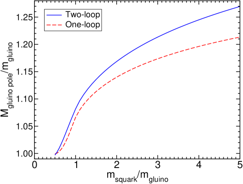
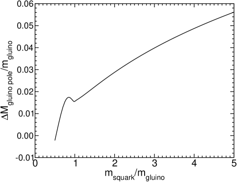
Figure 6: The SUSYQCD corrections to the gluino pole mass $M_{\tilde{g}}$, in the simplifying approximation of degenerate squarks, with no squark mixing or quark masses and Yukawa and electroweak effects neglected for simplicity. Here $m_{\rm squark}\equiv m_{\tilde{q}}$ and $m_{\rm gluino}\equiv m_{\tilde{g}}$ (often seen in the literature as $M_{3}$) are the tree-level running $\overline{\rm DR}^{\prime}$ squark and gluino mass parameters, all evaluated at a renormalization scale $Q=m_{\tilde{g}}(Q)$, and $M_{{\rm gluino}\,{\rm pole}}\equiv M_{\tilde{g}}$ is the square root of the real part of the pole mass. In the first panel, the dashed line is the one-loop result, and the solid line is the two-loop result, for the ratio of the gluino pole mass to the running gluino mass evaluated at itself. The second panel shows the difference between the two-loop and one-loop results. The computations were done by specializing eqs. (5.4)-(5.10) in the text, using $\alpha_{S}(Q)=g_{3}^{2}/4\pi=0.095$.

Also for simplicity, the top quark mass is neglected. In most realistic models of supersymmetry breaking, most of the squark masses are larger than about $0.8m_{\tilde{g}}$. Then the two-loop contribution to the gluino pole mass is positive, and from 1% to 2% for comparable gluino and squark masses, but it is larger when $m_{\tilde{q}}\gg m_{\tilde{g}}$.

The scale-dependence of the calculated pole mass is shown in fig. 7.

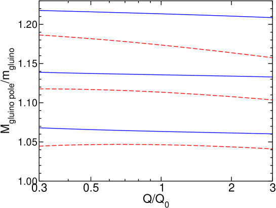
Figure 7: The scale-dependence of the computed gluino pole mass $M_{{\rm gluino}\,{\rm pole}}\equiv M_{\tilde{g}}$, in the simplifying approximation of degenerate squarks with no squark mixing or quark masses and Yukawa and electroweak effects. Here the top pair of lines are for $m_{\tilde{q}}(Q_{0})/m_{\tilde{g}}(Q_{0})=3$, the middle pair for $m_{\tilde{q}}(Q_{0})/m_{\tilde{g}}(Q_{0})=1.5$, and the bottom pair for $m_{\tilde{q}}(Q_{0})/m_{\tilde{g}}(Q_{0})=0.9$, where $m_{\tilde{g}}$ and $m_{\tilde{q}}$ are the running gluino and squark mass parameters evaluated at a reference renormalization scale $Q_{0}=m_{\tilde{g}}(Q_{0})$, with $\alpha_{S}(Q_{0})=g_{3}^{2}/4\pi=0.095$. In each case, the solid line is the two-loop result, and the dashed line is the one-loop result. The parameters $m_{\tilde{g}}$, $m_{\tilde{q}}$, and $\alpha_{S}$ are each run from the reference scale $Q_{0}$ to the scale $Q$ using two-loop renormalization group equations, and the gluino pole mass is then recomputed. The computations were done by specializing eqs. (5.4)-(5.10) in the text.

To make this graph, a reference renormalization scale $Q_{0}$ is chosen such that the running gluino mass evaluated there is equal to it, i.e. $Q_{0}=m_{\tilde{g}}(Q_{0})$. Then, for three different values of the ratio $m_{\tilde{q}}/m_{\tilde{g}}$ at the scale $Q_{0}$, namely 0.9, 1.5 and 3.0, the one-loop and two-loop gluino pole masses are computed as a function of $Q$. To do this, the relevant running parameters $m_{\tilde{g}}$, $m_{\tilde{q}}$, and $\alpha_{S}=g_{3}^{2}/4\pi$ are evolved using their two-loop renormalization group equations from $Q_{0}$ to $Q$, and then the pole mass is recomputed using eqs. (5.4)-(5.10). In the ideal case, the lines shown would be exactly horizontal. The scale dependence of the one-loop and two-loop results is about the same if the gluino mass is less than or about equal to the squark masses (as for example in gaugino-mass dominated or “no-scale” models). For heavier squark masses, it is significantly improved by going to two-loop order. Note that as usual, the scale-dependence of the one-loop approximation is considerably less than the difference between the two-loop and one-loop results. This strongly suggests that the scale-dependence should not be used as an indicator of the accuracy of the two-loop approximation either. A naive estimate of the size of the three-loop SUSYQCD contribution to the gluino pole mass can be obtained by considering the cube of the one-loop fractional contribution, and so is perhaps of the order of a few tenths of a per cent.

As mentioned above, results equivalent to those above in the limit of no squark mixing have previously been obtained independently by Y. Yamada in Yamada:2005ua , where numerical results were given and the analytical form for the pole mass of the gluino was shown explicitly in the limit $m_{\tilde{q}}\gg m_{\tilde{g}}$. I have checked that the results found here do agree with those in ref. Yamada:2005ua . (When comparing the numerical results, it is useful to note that small differences, formally of three-loop order, arise due to the fact that the present paper works in terms of perturbative corrections to the pole squared mass, while ref. Yamada:2005ua computed results for the pole mass.)

Further accuracy can be obtained by including the contributions of Feynman diagrams that are of order $\alpha_{S}$ times Yukawa or electroweak couplings squared. Such corrections could be particularly important if the gluino is relatively light, since we are working in a non-decoupling scheme. These results are implicitly contained above in section IV; obtaining their explicit form is only a matter of plugging in the couplings and masses of the MSSM. I will not do that here, because this paper already contains plenty of lengthy formulas, but only note that it can be done straightforwardly by use of a symbolic manipulation program, for example.

V.2 SUSYQCD corrections to quark masses in minimal supersymmetry

As another application of the general results above, consider the relation between the running and pole masses of the quarks in the MSSM, found earlier in quarkpoleSUSYa ; quarkpoleSUSYb ; Bednyakov:2005kt . Using the results of the present paper, I find for the top quark:

$$M^{2}_{t}-i\Gamma_{t}M_{t} = m^{2}_{t}+\frac{1}{16\pi^{2}}\widetilde{\Pi}^{(1)}_{t}+\frac{g_{3}^{4}}{(16\pi^{2})^{2}}\widetilde{\Pi}^{(2)}_{t}$$ (5.11)

where:

$$\widetilde{\Pi}^{(1)}_{t} = g_{3}^{2}C_{q}\bigl{\{}m_{t}^{2}(10-6{\overline{\rm ln}}m_{t}^{2})+2{\rm B}_{FS}(\tilde{g},\tilde{t}_{j})-4{\rm Re}[L_{\tilde{t}_{j}}R_{\tilde{t}_{j}}^{*}]m_{t}m_{\tilde{g}}{\rm B}_{{\overline{F}}S}(\tilde{g},\tilde{t}_{j})\bigr{\}}+2|Y_{t\overline{t}\phi_{j}^{0}}|^{2}{\rm B}_{FS}(t,\phi_{j}^{0})$$ (5.12)

$$+2{\rm Re}[(Y_{t\overline{t}\phi_{j}^{0}})^{2}]{\rm B}_{{\overline{F}}S}(t,\phi_{j}^{0})+(|Y_{\overline{t}b\phi_{j}^{+}}|^{2}+|Y_{\overline{b}t\phi_{j}^{-}}|^{2}){\rm B}_{FS}(b,\phi_{j}^{+})+2{\rm Re}[Y_{\overline{t}b\phi_{j}^{+}}Y_{\overline{b}t\phi_{j}^{-}}]m_{b}m_{t}{\rm B}_{{\overline{F}}S}(b,\phi_{j}^{+})$$

$$+(|Y_{t\tilde{N}_{i}\tilde{t}_{j}^{*}}|^{2}+|Y_{\overline{t}\tilde{N}_{i}\tilde{t}_{j}}|^{2}){\rm B}_{FS}(\tilde{N}_{i},\tilde{t}_{j})+2{\rm Re}[Y_{t\tilde{N}_{i}\tilde{t}_{j}^{*}}Y_{\overline{t}\tilde{N}_{i}\tilde{t}_{j}}]m_{t}m_{\tilde{N}_{i}}{\rm B}_{{\overline{F}}S}(\tilde{N}_{i},\tilde{t}_{j})$$

$$+(|Y_{t\tilde{C}_{i}\tilde{b}_{j}^{*}}|^{2}+|Y_{\overline{t}\tilde{C}_{i}\tilde{b}_{j}}|^{2}){\rm B}_{FS}(\tilde{C}_{i},\tilde{b}_{j})+2{\rm Re}[Y_{t\tilde{C}_{i}\tilde{b}_{j}^{*}}Y_{\overline{t}\tilde{C}_{i}\tilde{b}_{j}}]m_{t}m_{\tilde{C}_{i}}{\rm B}_{{\overline{F}}S}(\tilde{C}_{i},\tilde{b}_{j})$$

$$+\frac{4}{9}e^{2}m_{t}^{2}[10-6{\overline{\rm ln}}m_{t}^{2}]+\bigl{[}(g^{2}+g^{\prime 2})/4-2Q_{t}T_{3}^{t}g^{\prime 2}+2Q_{t}^{2}g^{\prime 4}/(g^{2}+g^{\prime 2})\bigr{]}{\rm B}_{FV}(t,Z)$$

$$+2Q_{t}g^{\prime 2}\bigl{[}Q_{t}g^{\prime 2}/(g^{2}+g^{\prime 2})-T_{3}^{t}\bigr{]}{\rm B}_{{\overline{F}}V}(t,Z)+g^{2}{\rm B}_{FV}(b,W)/2,$$

$$\widetilde{\Pi}^{(2)}_{t} = C_{q}(8C_{q}-4C_{G})\Bigl{\{}L_{\tilde{t}_{j}}R_{\tilde{t}_{j}}^{*}L_{\tilde{t}_{k}}^{*}R_{\tilde{t}_{k}}{\rm M}_{SFFSF}(\tilde{t}_{j},\tilde{g},\tilde{g},\tilde{t}_{k},t)+|L_{\tilde{t}_{j}}R_{\tilde{t}_{k}}|^{2}m_{t}^{2}{\rm M}_{SFFS{\overline{F}}}(\tilde{t}_{j},\tilde{g},\tilde{g},\tilde{t}_{k},t)$$ (5.13)

$$-{\rm Re}[L_{\tilde{t}_{k}}R_{\tilde{t}_{k}}^{*}]m_{t}m_{\tilde{g}}{\rm M}_{SF{\overline{F}}SF}(\tilde{t}_{j},\tilde{g},\tilde{g},\tilde{t}_{k},t)+\frac{1}{2}(|L_{\tilde{t}_{j}}L_{\tilde{t}_{k}}|^{2}+|R_{\tilde{t}_{j}}R_{\tilde{t}_{k}}|^{2})m_{\tilde{g}}^{2}{\rm M}_{S{\overline{F}}{\overline{F}}SF}(\tilde{t}_{j},\tilde{g},\tilde{g},\tilde{t}_{k},t)$$

$$-{\rm Re}[L_{\tilde{t}_{j}}R_{\tilde{t}_{j}}^{*}]m_{t}m_{\tilde{g}}{\rm M}_{SF{\overline{F}}S{\overline{F}}}(\tilde{t}_{j},\tilde{g},\tilde{g},\tilde{t}_{k},t)+{\rm Re}[L_{\tilde{t}_{j}}R_{\tilde{t}_{j}}^{*}L_{\tilde{t}_{k}}R_{\tilde{t}_{k}}^{*}]m_{t}^{2}m_{\tilde{g}}^{2}{\rm M}_{S{\overline{F}}{\overline{F}}S{\overline{F}}}(\tilde{t}_{j},\tilde{g},\tilde{g},\tilde{t}_{k},t)\Bigr{\}}$$

$$+8C_{q}I_{q}\Bigl{\{}\frac{1}{2}{\rm V}_{SFFFS}(\tilde{t}_{j},\tilde{g},\tilde{g},q,\tilde{q}_{k})+2{\rm Re}[L_{\tilde{t}_{j}}R_{\tilde{t}_{j}}^{*}L_{\tilde{q}_{k}}^{*}R_{\tilde{q}_{k}}]m_{t}m_{q}{\rm V}_{SFF{\overline{F}}S}(\tilde{t}_{j},\tilde{g},\tilde{g},q,\tilde{q}_{k})$$

$$-2{\rm Re}[L_{\tilde{t}_{j}}R_{\tilde{t}_{j}}^{*}]m_{t}m_{\tilde{g}}{\rm V}_{SF{\overline{F}}FS}(\tilde{t}_{j},\tilde{g},\tilde{g},q,\tilde{q}_{k})+\frac{1}{2}m_{\tilde{g}}^{2}{\rm V}_{S{\overline{F}}{\overline{F}}FS}(\tilde{t}_{j},\tilde{g},\tilde{g},q,\tilde{q}_{k})$$

$$-2{\rm Re}[L_{\tilde{q}_{k}}R_{\tilde{q}_{k}}^{*}]m_{q}m_{\tilde{g}}{\rm V}_{SF{\overline{F}}{\overline{F}}S}(\tilde{t}_{j},\tilde{g},\tilde{g},q,\tilde{q}_{k})+2{\rm Re}[L_{\tilde{t}_{j}}R_{\tilde{t}_{j}}^{*}L_{\tilde{q}_{k}}R_{\tilde{q}_{k}}^{*}]m_{q}m_{t}m^{2}_{\tilde{g}}{\rm V}_{S{\overline{F}}{\overline{F}}{\overline{F}}S}(\tilde{t}_{j},\tilde{g},\tilde{g},q,\tilde{q}_{k})\Bigr{\}}$$

$$+4C_{q}^{2}\Bigl{\{}{\rm V}_{FSSFF}(\tilde{g},\tilde{t}_{j},\tilde{t}_{j},t,\tilde{g})-2{\rm Re}[L_{\tilde{t}_{j}}R_{\tilde{t}_{j}}^{*}]m_{t}m_{\tilde{g}}[{\rm V}_{{\overline{F}}SSFF}(\tilde{g},\tilde{t}_{j},\tilde{t}_{j},t,\tilde{g})+{\rm V}_{FSS{\overline{F}}{\overline{F}}}(\tilde{g},\tilde{t}_{j},\tilde{t}_{j},t,\tilde{g})]$$

$$+2({\rm Re}[L_{\tilde{t}_{j}}R_{\tilde{t}_{j}}^{*}L_{\tilde{t}_{k}}R_{\tilde{t}_{k}}^{*}]+|L_{\tilde{t}_{j}}R_{\tilde{t}_{k}}|^{2})m_{t}^{2}m_{\tilde{g}}^{2}{\rm V}_{{\overline{F}}SS{\overline{F}}{\overline{F}}}(\tilde{g},\tilde{t}_{j},\tilde{t}_{k},t,\tilde{g})]+\frac{1}{2}|L_{\tilde{t}_{j}}L_{\tilde{t}_{k}}^{*}-R_{\tilde{t}_{j}}R_{\tilde{t}_{k}}^{*}|^{2}{\rm Y}_{FSSS}(\tilde{g},\tilde{t}_{j},\tilde{t}_{j},\tilde{t}_{k})$$

$$-{\rm Re}[L_{\tilde{t}_{j}}^{*}R_{\tilde{t}_{k}}(L_{\tilde{t}_{j}}L_{\tilde{t}_{n}}^{*}-R_{\tilde{t}_{j}}R_{\tilde{t}_{n}}^{*})(L_{\tilde{t}_{n}}L_{\tilde{t}_{k}}^{*}-R_{\tilde{t}_{n}}R_{\tilde{t}_{k}}^{*})]m_{t}m_{\tilde{g}}{\rm Y}_{{\overline{F}}SSS}(\tilde{g},\tilde{t}_{j},\tilde{t}_{k},\tilde{t}_{n})$$

$$+\bigl{\{}{\rm B}_{FS}(\tilde{g},\tilde{t}_{j})-2{\rm Re}[L_{\tilde{t}_{j}}R_{\tilde{t}_{j}}^{*}]m_{t}m_{\tilde{g}}{\rm B}_{{\overline{F}}S}(\tilde{g},\tilde{t}_{j})\bigr{\}}\bigl{\{}{\rm B}^{\prime}_{FS}(\tilde{g},\tilde{t}_{k})-2{\rm Re}[L_{\tilde{t}_{k}}R_{\tilde{t}_{k}}^{*}]m_{t}m_{\tilde{g}}{\rm B}^{\prime}_{{\overline{F}}S}(\tilde{g},\tilde{t}_{k})\bigr{\}}$$

$$+{\rm Re}[L_{\tilde{t}_{j}}R_{\tilde{t}_{j}}^{*}]{\rm Re}[L_{\tilde{t}_{k}}R_{\tilde{t}_{k}}^{*}]m_{\tilde{g}}^{2}{\rm B}_{{\overline{F}}S}(\tilde{g},\tilde{t}_{j}){\rm B}_{{\overline{F}}S}(\tilde{g},\tilde{t}_{k})-|L_{\tilde{t}_{j}}R_{\tilde{t}_{k}}|^{2}{\rm B}_{FS}(\tilde{g},\tilde{t}_{j}){\rm B}_{FS}(\tilde{g},\tilde{t}_{k})/m_{t}^{2}\Bigr{\}}$$

$$+C_{G}C_{q}f_{1}(t,\tilde{g},\tilde{t}_{j})+2(C_{G}-C_{q})C_{q}f_{2}(t,\tilde{g},\tilde{t}_{j})+2C_{q}^{2}f_{3}(t,\tilde{g},\tilde{t}_{j})$$

$$-2C_{q}{\rm Re}[L_{\tilde{t}_{j}}R_{\tilde{t}_{j}}^{*}]m_{t}m_{\tilde{g}}\bigl{\{}C_{G}f_{4}(t,\tilde{g},\tilde{t}_{j})+2(C_{G}-C_{q})f_{5}(t,\tilde{g},\tilde{t}_{j})+2C_{q}f_{6}(t,\tilde{g},\tilde{t}_{j})\bigr{\}}$$

$$+C_{q}^{2}F_{1}(t)+C_{G}C_{q}\bigl{[}F_{2}(t)+F_{3}(t,\tilde{g})\bigr{]}+C_{q}I_{q}\bigl{[}2F_{3}(t,q)+F_{4}(t,\tilde{q}_{j})\bigr{]}.$$

The gauge group constants are $C_{q}=4/3$, $C_{G}=3$, $I_{q}=1/2$, $Q_{t}=2/3$ and $T_{3}^{t}=1/2$. The results for the bottom quark can be obtained by taking $t\leftrightarrow b$ everywhere, with $Q_{t}\rightarrow Q_{b}=-1/3$ and $T_{3}^{t}\rightarrow T_{3}^{b}=-1/2$. The one-loop part given by eq. (5.12) was given in a different notation in PBMZ . It includes all effects, including those due to the exchange of virtual neutral Higgs scalars [$\phi^{0}_{j}=(h^{0},H^{0},G^{0},A^{0})$ for $j=1,2,3,4$] charged Higgs scalars [$\phi^{\pm}_{j}=(G^{\pm},H^{\pm})$ for $j=1,2$], neutralinos [$\tilde{N}_{j}$ for $j=1,2,3,4$], and charginos [$\tilde{C}_{j}$ for $j=1,2$] and top and bottom squarks. In each of the loop integral functions in eqs. (5.12) and (5.13), one should take $s=m_{t}^{2}$ with an infinitesimal positive imaginary part. [Here I have only listed the pure SUSYQCD corrections explicitly in the two-loop part, but the corrections involving Yukawa couplings and scalar trilinear couplings are also given implicitly by specializing the results of section IV.]

I have checked that the result given above is consistent with the two-loop renormalization group equations, in the sense that the pole mass is invariant under changes in the renormalization scale given by the two-loop SUSYQCD renormalization group equation for the top quark mass. As another non-trivial consistency check, I have verified that in the (clearly unrealistic) supersymmetric limit, the top-quark pole mass given above is precisely equal to the top-squark pole mass as found in eqs. (5.28)-(5.30) of ref. Martin:2005eg . [In the published and original preprint versions of that paper, the term in eq. (5.30) proportional to $I_{q}$ was missing a factor of 2.]

The two-loop SUSYQCD contribution and Yukawa contributions had already been found in refs. quarkpoleSUSYa ; quarkpoleSUSYb ; Bednyakov:2005kt , using a method in which loop integrals are evaluated using an expansion in small mass hierarchies. In principle, the present paper generalizes this somewhat, since here I use two-loop integral basis functions without mass expansions. However, as was recently pointed out in Bednyakov:2005kt , the actual top and bottom quark masses are such that the leading terms in the mass expansion already give an extremely good approximation throughout most of the parameter space left available to supersymmetry. I have also checked agreement with eqs. (57)-(62) in ref. quarkpoleSUSYa . References quarkpoleSUSYa ; quarkpoleSUSYb ; Bednyakov:2005kt also include an extensive study of the impact of the two-loop top and bottom quark mass corrections in the MSSM.

V.3 SUSYQCD corrections to neutralino and chargino masses

In this section, I present the two-loop corrections to neutralino and chargino masses that involve the strong coupling. These arise from gluon and gluino propagator lines added to the one-loop Feynman diagrams that involve quarks and squarks, and so are parametrically of order $\alpha_{S}y_{t}^{2}$, $\alpha_{S}y_{b}^{2}$, $\alpha_{S}g^{2}$, $\alpha_{S}gg^{\prime}$ and $\alpha_{S}g^{\prime 2}$. These two-loop contributions are evaluated by specializing the results above, and do not require the neglect of $W$ and $Z$ boson masses.

Using the general results of sections III and IV, one can write the neutralino pole masses as:

$$M_{\tilde{N}_{i}}^{2}-i\Gamma_{\tilde{N}_{i}}M_{\tilde{N}_{i}}=m_{\tilde{N}_{i}}^{2}+\frac{1}{16\pi^{2}}\widetilde{\Pi}^{(1)}_{\tilde{N}_{i}}+\frac{1}{(16\pi^{2})^{2}}\widetilde{\Pi}^{(2)}_{\tilde{N}_{i}},$$ (5.14)

for $i=1,2,3,4$, where $m_{\tilde{N}_{i}}^{2}$ are the tree-level squared mass eigenvalues, and the one-loop part is Pierce ; PBMZ ,

$$\widetilde{\Pi}^{(1)}_{\tilde{N}_{i}} = 2n_{f}\bigl{(}|Y_{f\tilde{N}_{i}\tilde{f}_{j}^{*}}|^{2}+|Y_{\overline{f}\tilde{N}_{i}\tilde{f}_{j}}|^{2}\bigr{)}{\rm B}_{FS}(f,\tilde{f}_{j})+4n_{f}{\rm Re}[Y_{f\tilde{N}_{i}\tilde{f}_{j}^{*}}Y_{\overline{f}\tilde{N}_{i}\tilde{f}_{j}}]m_{\tilde{N}_{i}}m_{f}{\rm B}_{{\overline{F}}S}(f,\tilde{f}_{j})$$ (5.15)

$$+2|Y_{\tilde{N}_{i}\tilde{N}_{j}\phi^{0}_{k}}|^{2}{\rm B}_{FS}(\tilde{N}_{j},\phi^{0}_{k})+2{\rm Re}[(Y_{\tilde{N}_{i}\tilde{N}_{j}\phi^{0}_{k}})^{2}]m_{\tilde{N}_{i}}m_{\tilde{N}_{j}}{\rm B}_{{\overline{F}}S}(\tilde{N}_{j},\phi^{0}_{k})$$

$$+2(|Y_{\tilde{C}_{j}^{+}\tilde{N}_{i}\phi_{k}^{-}}|^{2}+|Y_{\tilde{C}_{j}^{-}\tilde{N}_{i}\phi_{k}^{+}}|^{2}){\rm B}_{FS}(\tilde{C}_{j},\phi_{k}^{+})+4{\rm Re}[Y_{\tilde{C}_{j}^{+}\tilde{N}_{i}\phi_{k}^{-}}Y_{\tilde{C}_{j}^{-}\tilde{N}_{i}\phi_{k}^{+}}]m_{\tilde{N}_{i}}m_{\tilde{C}_{j}}{\rm B}_{{\overline{F}}S}(\tilde{C}_{j},\phi_{k}^{+})$$

$$+2(g^{2}+g^{\prime 2})\left\{|O^{\prime\prime L}_{ij}|^{2}{\rm B}_{FV}(\tilde{N}_{j},Z)-{\rm Re}[(O^{\prime\prime L}_{ij})^{2}]m_{\tilde{N}_{i}}m_{\tilde{N}_{j}}{\rm B}_{{\overline{F}}V}(\tilde{N}_{j},Z)\right\}$$

$$+2g^{2}(|O^{L}_{ij}|^{2}+|O^{R}_{ij}|^{2}){\rm B}_{FV}(\tilde{C}_{j},W)+4g^{2}{\rm Re}[O^{L}_{ij}O^{R*}_{ij}]m_{\tilde{N}_{i}}m_{\tilde{C}_{j}}{\rm B}_{{\overline{F}}V}(\tilde{C}_{j},W),$$

and the two-loop SUSYQCD part (i.e., the part involving the strong interactions) is

$$\widetilde{\Pi}^{(2)}_{\tilde{N}_{i}} = 16g_{3}^{2}\Bigl{\{}\frac{1}{2}(|Y_{q\tilde{N}_{i}\tilde{q}_{j}^{*}}|^{2}+|Y_{\overline{q}\tilde{N}_{i}\tilde{q}_{j}}|^{2})f_{1}(\tilde{N}_{i},q,\tilde{q}_{j})+{\rm Re}[Y_{q\tilde{N}_{i}\tilde{q}_{j}^{*}}Y_{\overline{q}\tilde{N}_{i}\tilde{q}_{j}}]m_{\tilde{N}_{i}}m_{q}f_{4}(\tilde{N}_{i},q,\tilde{q}_{j})$$ (5.16)

$$-2{\rm Re}[Y_{q\tilde{N}_{i}\tilde{q}_{j}^{*}}Y_{\overline{q}\tilde{N}_{i}\tilde{q}_{k}}^{*}R_{\tilde{q}_{j}}L_{\tilde{q}_{k}}]{\rm M}_{SFFSF}(\tilde{q}_{j},q,q,\tilde{q}_{k},\tilde{g})-2{\rm Re}[Y_{q\tilde{N}_{i}\tilde{q}_{j}^{*}}Y_{\overline{q}\tilde{N}_{i}\tilde{q}_{k}}^{*}L_{\tilde{q}_{j}}R_{\tilde{q}_{k}}]m_{q}^{2}{\rm M}_{S{\overline{F}}{\overline{F}}SF}(\tilde{q}_{j},q,q,\tilde{q}_{k},\tilde{g})$$

$$+{\rm Re}[Y_{q\tilde{N}_{i}\tilde{q}_{j}^{*}}Y_{q\tilde{N}_{i}\tilde{q}_{k}^{*}}L_{\tilde{q}_{j}}L_{\tilde{q}_{k}}+Y_{\overline{q}\tilde{N}_{i}\tilde{q}_{j}}Y_{\overline{q}\tilde{N}_{i}\tilde{q}_{k}}R_{\tilde{q}_{j}}^{*}R_{\tilde{q}_{k}}^{*}]m_{\tilde{N}_{i}}m_{\tilde{g}}{\rm M}_{SFFS{\overline{F}}}(\tilde{q}_{j},q,q,\tilde{q}_{k},\tilde{g})$$

$$-2{\rm Re}[Y_{q\tilde{N}_{i}\tilde{q}_{j}^{*}}Y_{q\tilde{N}_{i}\tilde{q}_{k}^{*}}L_{\tilde{q}_{j}}R_{\tilde{q}_{k}}+Y_{\overline{q}\tilde{N}_{i}\tilde{q}_{j}}Y_{\overline{q}\tilde{N}_{i}\tilde{q}_{k}}R_{\tilde{q}_{j}}^{*}L_{\tilde{q}_{k}}^{*}]m_{\tilde{N}_{i}}m_{q}{\rm M}_{SF{\overline{F}}SF}(\tilde{q}_{j},q,q,\tilde{q}_{k},\tilde{g})$$

$$+2{\rm Re}[Y_{q\tilde{N}_{i}\tilde{q}_{j}^{*}}Y_{\overline{q}\tilde{N}_{i}\tilde{q}_{k}}^{*}R_{\tilde{q}_{j}}R_{\tilde{q}_{k}}+Y_{\overline{q}\tilde{N}_{i}\tilde{q}_{j}}^{*}Y_{q\tilde{N}_{i}\tilde{q}_{k}^{*}}L_{\tilde{q}_{j}}L_{\tilde{q}_{k}}]m_{q}m_{\tilde{g}}{\rm M}_{SF{\overline{F}}S{\overline{F}}}(\tilde{q}_{j},q,q,\tilde{q}_{k},\tilde{g})$$

$$+{\rm Re}[Y_{q\tilde{N}_{i}\tilde{q}_{j}^{*}}Y_{q\tilde{N}_{i}\tilde{q}_{k}^{*}}R_{\tilde{q}_{j}}R_{\tilde{q}_{k}}+Y_{\overline{q}\tilde{N}_{i}\tilde{q}_{j}}Y_{\overline{q}\tilde{N}_{i}\tilde{q}_{k}}L_{\tilde{q}_{j}}^{*}L_{\tilde{q}_{k}}^{*}]m_{\tilde{N}_{i}}m_{\tilde{g}}m_{q}^{2}{\rm M}_{S{\overline{F}}{\overline{F}}S{\overline{F}}}(\tilde{q}_{j},q,q,\tilde{q}_{k},\tilde{g})$$

$$+(|Y_{q\tilde{N}_{i}\tilde{q}_{j}^{*}}|^{2}+|Y_{\overline{q}\tilde{N}_{i}\tilde{q}_{j}}|^{2}){\rm V}_{FSSFF}(q,\tilde{q}_{j},\tilde{q}_{j},\tilde{g},q)+2{\rm Re}[Y_{q\tilde{N}_{i}\tilde{q}_{j}^{*}}Y_{\overline{q}\tilde{N}_{i}\tilde{q}_{j}}]m_{\tilde{N}_{i}}m_{q}{\rm V}_{{\overline{F}}SSFF}(q,\tilde{q}_{j},\tilde{q}_{j},\tilde{g},q)$$

$$-2{\rm Re}[(Y_{q\tilde{N}_{i}\tilde{q}_{j}^{*}}Y_{q\tilde{N}_{i}\tilde{q}_{k}^{*}}^{*}+Y_{\overline{q}\tilde{N}_{i}\tilde{q}_{j}}^{*}Y_{\overline{q}\tilde{N}_{i}\tilde{q}_{k}})R_{\tilde{q}_{j}}L_{\tilde{q}_{k}}^{*}]m_{q}m_{\tilde{g}}{\rm V}_{FSS{\overline{F}}{\overline{F}}}(q,\tilde{q}_{j},\tilde{q}_{k},\tilde{g},q)$$

$$-2{\rm Re}[Y_{q\tilde{N}_{i}\tilde{q}_{j}^{*}}Y_{\overline{q}\tilde{N}_{i}\tilde{q}_{k}}(R_{\tilde{q}_{j}}L_{\tilde{q}_{k}}^{*}+L_{\tilde{q}_{j}}R_{\tilde{q}_{k}}^{*})]m_{\tilde{N}_{i}}m_{q}^{2}m_{\tilde{g}}{\rm V}_{{\overline{F}}SS{\overline{F}}{\overline{F}}}(q,\tilde{q}_{j},\tilde{q}_{k},\tilde{g},q)$$

$$+(|Y_{q\tilde{N}_{i}\tilde{q}_{j}^{*}}L_{\tilde{q}_{k}}|^{2}+|Y_{\overline{q}\tilde{N}_{i}\tilde{q}_{j}}R_{\tilde{q}_{k}}|^{2}){\rm V}_{SFFFS}(\tilde{q}_{j},q,q,\tilde{g},\tilde{q}_{k})+2{\rm Re}[Y_{q\tilde{N}_{i}\tilde{q}_{j}^{*}}Y_{\overline{q}\tilde{N}_{i}\tilde{q}_{j}}]m_{\tilde{N}_{i}}m_{q}{\rm V}_{SF{\overline{F}}FS}(\tilde{q}_{j},q,q,\tilde{g},\tilde{q}_{k})$$

$$-2{\rm Re}[Y_{q\tilde{N}_{i}\tilde{q}_{j}^{*}}Y_{\overline{q}\tilde{N}_{i}\tilde{q}_{j}}L_{\tilde{q}_{k}}R_{\tilde{q}_{k}}^{*}]m_{\tilde{N}_{i}}m_{\tilde{g}}{\rm V}_{SFF{\overline{F}}S}(\tilde{q}_{j},q,q,\tilde{g},\tilde{q}_{k})$$

$$+(|Y_{q\tilde{N}_{i}\tilde{q}_{j}^{*}}R_{\tilde{q}_{k}}|^{2}+|Y_{\overline{q}\tilde{N}_{i}\tilde{q}_{j}}L_{\tilde{q}_{k}}|^{2})m_{q}^{2}{\rm V}_{S{\overline{F}}{\overline{F}}FS}(\tilde{q}_{j},q,q,\tilde{g},\tilde{q}_{k})$$

$$-2(|Y_{q\tilde{N}_{i}\tilde{q}_{j}^{*}}|^{2}+|Y_{\overline{q}\tilde{N}_{i}\tilde{q}_{j}}|^{2}){\rm Re}[L_{\tilde{q}_{k}}R_{\tilde{q}_{k}}^{*}]m_{q}m_{\tilde{g}}{\rm V}_{SF{\overline{F}}{\overline{F}}S}(\tilde{q}_{j},q,q,\tilde{g},\tilde{q}_{k})$$

$$-2{\rm Re}[Y_{q\tilde{N}_{i}\tilde{q}_{j}^{*}}Y_{\overline{q}\tilde{N}_{i}\tilde{q}_{j}}R_{\tilde{q}_{k}}L_{\tilde{q}_{k}}^{*}]m_{\tilde{N}_{i}}m_{q}^{2}m_{\tilde{g}}{\rm V}_{S{\overline{F}}{\overline{F}}{\overline{F}}S}(\tilde{q}_{j},q,q,\tilde{g},\tilde{q}_{k})$$

$$+\frac{1}{2}(L_{\tilde{q}_{j}}L_{\tilde{q}_{n}}^{*}-R_{\tilde{q}_{j}}R_{\tilde{q}_{n}}^{*})(L_{\tilde{q}_{n}}L_{\tilde{q}_{k}}^{*}-R_{\tilde{q}_{n}}R_{\tilde{q}_{k}}^{*})\bigl{[}(Y_{q\tilde{N}_{i}\tilde{q}_{j}^{*}}Y_{q\tilde{N}_{i}\tilde{q}_{k}^{*}}^{*}+Y_{\overline{q}\tilde{N}_{i}\tilde{q}_{j}}^{*}Y_{\overline{q}\tilde{N}_{i}\tilde{q}_{k}}){\rm Y}_{FSSS}(q,\tilde{q}_{j},\tilde{q}_{k},\tilde{q}_{n})$$

$$+(Y_{q\tilde{N}_{i}\tilde{q}_{j}^{*}}Y_{\overline{q}\tilde{N}_{i}\tilde{q}_{k}}+Y_{\overline{q}\tilde{N}_{i}\tilde{q}_{j}}^{*}Y_{q\tilde{N}_{i}\tilde{q}_{k}^{*}}^{*})m_{\tilde{N}_{i}}m_{q}{\rm Y}_{{\overline{F}}SSS}(q,\tilde{q}_{j},\tilde{q}_{k},\tilde{q}_{n})\bigr{]}\Bigr{\}}.$$

In eq. (5.15), $f$ is summed over the symbols $e$, $\mu$, $\tau$, $\nu_{e}$, $\nu_{\mu}$, $\nu_{\tau}$, $u$, $d$, $c$, $s$, $t$, $b$, with $n_{f}=1$ for leptons and $3$ for quarks, and in eq. (5.16) the symbol $q$ is summed over $u$, $d$, $c$, $s$, $t$, $b$. The indices $j,k,n$ are each summed over the appropriate ranges ($1,2$ for squarks, sleptons, charginos, and charged Higgs scalars, $1,2,3,4$ for neutralinos and neutral Higgs scalars, including the Goldstone bosons) wherever they appear. The masses and couplings appearing on the right-hand side are always running renormalized $\overline{\rm DR}^{\prime}$ parameters. In all of the self-energy functions appearing in eqs. (5.15) and (5.16), the external momentum invariant is $s=m^{2}_{\tilde{N}_{i}}$ with an infinitesimal positive imaginary part.

Similarly, the pole masses for charginos in the MSSM can be written as

$$M_{\tilde{C}_{i}}^{2}-i\Gamma_{\tilde{C}_{i}}M_{\tilde{C}_{i}}=m_{\tilde{C}_{i}}^{2}+\frac{1}{16\pi^{2}}\widetilde{\Pi}^{(1)}_{\tilde{C}_{i}}+\frac{1}{(16\pi^{2})^{2}}\widetilde{\Pi}^{(2)}_{\tilde{C}_{i}},$$ (5.17)

for $i=1,2$, where $m_{\tilde{C}_{i}}^{2}$ are the tree-level squared mass eigenvalues, and the one-loop part is Pierce ; PBMZ ,

$$\widetilde{\Pi}^{(1)}_{\tilde{C}_{i}} = n_{f}(|Y_{f\tilde{C}_{i}\tilde{F}_{j}^{*}}|^{2}+|Y_{\overline{f}\tilde{C}_{i}\tilde{F}_{j}}|^{2}){\rm B}_{FS}(f,\tilde{F}_{j})+2n_{f}{\rm Re}[Y_{f\tilde{C}_{i}\tilde{F}_{j}^{*}}Y_{\overline{f}\tilde{C}_{i}\tilde{F}_{j}}]m_{\tilde{C}_{i}}m_{f}{\rm B}_{{\overline{F}}S}(f,\tilde{F}_{j})$$ (5.18)

$$+(|Y_{\tilde{C}_{i}^{+}\tilde{N}_{j}\phi_{k}^{-}}|^{2}+|Y_{\tilde{C}_{i}^{-}\tilde{N}_{j}\phi_{k}^{+}}|^{2}){\rm B}_{FS}(\tilde{N}_{j},\phi_{k}^{+})+2{\rm Re}[Y_{\tilde{C}_{i}^{+}\tilde{N}_{j}\phi_{k}^{-}}Y_{\tilde{C}_{i}^{-}\tilde{N}_{j}\phi_{k}^{+}}]m_{\tilde{C}_{i}}m_{\tilde{N}_{j}}{\rm B}_{{\overline{F}}S}(\tilde{N}_{j},\phi_{k}^{+})$$

$$+(|Y_{\tilde{C}_{i}^{+}\tilde{C}_{j}^{-}\phi_{k}^{0}}|^{2}+|Y_{\tilde{C}_{j}^{+}\tilde{C}_{i}^{-}\phi_{k}^{0}}|^{2}){\rm B}_{FS}(\tilde{C}_{j},\phi_{k}^{0})+2{\rm Re}[Y_{\tilde{C}_{i}^{+}\tilde{C}_{j}^{-}\phi_{k}^{0}}Y_{\tilde{C}_{j}^{+}\tilde{C}_{i}^{-}\phi_{k}^{0}}]m_{\tilde{C}_{i}}m_{\tilde{C}_{j}}{\rm B}_{{\overline{F}}S}(\tilde{C}_{j},\phi_{k}^{0})$$

$$+e^{2}m^{2}_{\tilde{C}_{i}}[10-6{\overline{\rm ln}}m^{2}_{\tilde{C}_{i}}]+g^{2}(|O^{L}_{ji}|^{2}+|O^{R}_{ji}|^{2}){\rm B}_{FV}(\tilde{N}_{j},W)+2g^{2}{\rm Re}[O^{L}_{ji}O^{R*}_{ji}]m_{\tilde{C}_{i}}m_{\tilde{N}_{j}}{\rm B}_{{\overline{F}}V}(\tilde{N}_{j},W)$$

$$+(g^{2}+g^{\prime 2})\bigl{[}(|O^{\prime L}_{ij}|^{2}+|O^{\prime R}_{ij}|^{2}){\rm B}_{FV}(\tilde{C}_{j},Z)+2{\rm Re}[O^{\prime L}_{ji}O^{\prime R}_{ij}]m_{\tilde{C}_{i}}m_{\tilde{C}_{j}}{\rm B}_{FV}(\tilde{C}_{j},Z)\bigr{]},$$

and the two-loop part involving the strong interaction is

$$\widetilde{\Pi}^{(2)}_{\tilde{C}_{i}} = 8g_{3}^{2}\Bigl{\{}\frac{1}{2}(|Y_{q\tilde{C}_{i}\tilde{Q}_{j}^{*}}|^{2}+|Y_{\overline{q}\tilde{C}_{i}\tilde{Q}_{j}}|^{2})f_{1}(\tilde{C}_{i},q,\tilde{Q}_{j})+{\rm Re}[Y_{q\tilde{C}_{i}\tilde{Q}_{j}^{*}}Y_{\overline{q}\tilde{C}_{i}\tilde{Q}_{j}}]m_{\tilde{C}_{i}}m_{q}f_{4}(\tilde{C}_{i},q,\tilde{Q}_{j})$$ (5.19)

$$-2{\rm Re}[Y_{q\tilde{C}_{i}\tilde{Q}_{j}^{*}}Y_{\overline{Q}\tilde{C}_{i}\tilde{q}_{k}}^{*}R_{\tilde{Q}_{j}}L_{\tilde{q}_{k}}]{\rm M}_{SFFSF}(\tilde{Q}_{j},Q,q,\tilde{q}_{k},\tilde{g})$$

$$+{\rm Re}[Y_{q\tilde{C}_{i}\tilde{Q}_{j}^{*}}Y_{Q\tilde{C}_{i}\tilde{q}_{k}^{*}}L_{\tilde{Q}_{j}}L_{\tilde{q}_{k}}+Y_{\overline{q}\tilde{C}_{i}\tilde{Q}_{j}}Y_{\overline{Q}\tilde{C}_{i}\tilde{q}_{k}}R_{\tilde{Q}_{j}}^{*}R_{\tilde{q}_{k}}^{*}]m_{\tilde{C}_{i}}m_{\tilde{g}}{\rm M}_{SFFS{\overline{F}}}(\tilde{Q}_{j},Q,q,\tilde{q}_{k},\tilde{g})$$

$$-2{\rm Re}[Y_{q\tilde{C}_{i}\tilde{Q}_{j}^{*}}Y_{Q\tilde{C}_{i}\tilde{q}_{k}^{*}}L_{\tilde{Q}_{j}}R_{\tilde{q}_{k}}+Y_{\overline{q}\tilde{C}_{i}\tilde{Q}_{j}}Y_{\overline{Q}\tilde{C}_{i}\tilde{q}_{k}}R_{\tilde{Q}_{j}}^{*}L_{\tilde{q}_{k}}^{*}]m_{\tilde{C}_{i}}m_{q}{\rm M}_{SF{\overline{F}}SF}(\tilde{Q}_{j},Q,q,\tilde{q}_{k},\tilde{g})$$

$$-2{\rm Re}[Y_{q\tilde{C}_{i}\tilde{Q}_{j}^{*}}Y_{\overline{Q}\tilde{C}_{i}\tilde{q}_{k}}^{*}L_{\tilde{Q}_{j}}R_{\tilde{q}_{k}}]m_{q}m_{Q}{\rm M}_{S{\overline{F}}{\overline{F}}SF}(\tilde{Q}_{j},Q,q,\tilde{q}_{k},\tilde{g})$$

$$+2{\rm Re}[Y_{q\tilde{C}_{i}\tilde{Q}_{j}^{*}}Y_{\overline{Q}\tilde{C}_{i}\tilde{q}_{k}}^{*}R_{\tilde{Q}_{j}}R_{\tilde{q}_{k}}+Y_{\overline{q}\tilde{C}_{i}\tilde{Q}_{j}}^{*}Y_{Q\tilde{C}_{i}\tilde{q}_{k}^{*}}L_{\tilde{Q}_{j}}L_{\tilde{q}_{k}}]m_{q}m_{\tilde{g}}{\rm M}_{SF{\overline{F}}S{\overline{F}}}(\tilde{Q}_{j},Q,q,\tilde{q}_{k},\tilde{g})$$

$$+{\rm Re}[Y_{q\tilde{C}_{i}\tilde{Q}_{j}^{*}}Y_{Q\tilde{C}_{i}\tilde{q}_{k}^{*}}R_{\tilde{Q}_{j}}R_{\tilde{q}_{k}}+Y_{\overline{q}\tilde{C}_{i}\tilde{Q}_{j}}Y_{\overline{Q}\tilde{C}_{i}\tilde{q}_{k}}L_{\tilde{Q}_{j}}^{*}L_{\tilde{q}_{k}}^{*}]m_{\tilde{C}_{i}}m_{q}m_{Q}m_{\tilde{g}}{\rm M}_{S{\overline{F}}{\overline{F}}S{\overline{F}}}(\tilde{Q}_{j},Q,q,\tilde{q}_{k},\tilde{g})$$

$$+(|Y_{q\tilde{C}_{i}\tilde{Q}_{j}^{*}}|^{2}+|Y_{\overline{q}\tilde{C}_{i}\tilde{Q}_{j}}|^{2}){\rm V}_{FSSFF}(q,\tilde{Q}_{j},\tilde{Q}_{j},\tilde{g},Q)+2{\rm Re}[Y_{q\tilde{C}_{i}\tilde{Q}_{j}^{*}}Y_{\overline{q}\tilde{C}_{i}\tilde{Q}_{j}}]m_{\tilde{C}_{i}}m_{q}{\rm V}_{{\overline{F}}SSFF}(q,\tilde{Q}_{j},\tilde{Q}_{j},\tilde{g},Q)$$

$$-2{\rm Re}[(Y_{q\tilde{C}_{i}\tilde{Q}_{j}^{*}}Y_{q\tilde{C}_{i}\tilde{Q}_{k}^{*}}^{*}+Y_{\overline{q}\tilde{C}_{i}\tilde{Q}_{j}}^{*}Y_{\overline{q}\tilde{C}_{i}\tilde{Q}_{k}})L_{\tilde{Q}_{j}}R^{*}_{\tilde{Q}_{k}}]m_{Q}m_{\tilde{g}}{\rm V}_{FSS{\overline{F}}{\overline{F}}}(q,\tilde{Q}_{j},\tilde{Q}_{k},\tilde{g},Q)$$

$$-2{\rm Re}[Y_{q\tilde{C}_{i}\tilde{Q}_{j}^{*}}Y_{\overline{q}\tilde{C}_{i}\tilde{Q}_{k}}(L_{\tilde{Q}_{j}}R^{*}_{\tilde{Q}_{k}}+R_{\tilde{Q}_{j}}L^{*}_{\tilde{Q}_{k}})]m_{\tilde{C}_{i}}m_{q}m_{Q}m_{\tilde{g}}{\rm V}_{{\overline{F}}SS{\overline{F}}{\overline{F}}}(q,\tilde{Q}_{j},\tilde{Q}_{k},\tilde{g},Q)$$

$$+(|Y_{q\tilde{C}_{i}\tilde{Q}_{j}^{*}}L_{\tilde{q}_{k}}|^{2}+|Y_{\overline{q}\tilde{C}_{i}\tilde{Q}_{j}}R_{\tilde{q}_{k}}|^{2}){\rm V}_{SFFFS}(\tilde{Q}_{j},q,q,\tilde{g},\tilde{q}_{k})+2{\rm Re}[Y_{q\tilde{C}_{i}\tilde{Q}_{j}^{*}}Y_{\overline{q}\tilde{C}_{i}\tilde{Q}_{j}}]m_{\tilde{C}_{i}}m_{q}{\rm V}_{SF{\overline{F}}FS}(\tilde{Q}_{j},q,q,\tilde{g},\tilde{q}_{k})$$

$$-2{\rm Re}[Y_{q\tilde{C}_{i}\tilde{Q}_{j}^{*}}Y_{\overline{q}\tilde{C}_{i}\tilde{Q}_{j}}L_{\tilde{q}_{k}}R^{*}_{\tilde{q}_{k}}]m_{\tilde{C}_{i}}m_{\tilde{g}}{\rm V}_{SFF{\overline{F}}S}(\tilde{Q}_{j},q,q,\tilde{g},\tilde{q}_{k})$$

$$+(|Y_{q\tilde{C}_{i}\tilde{Q}_{j}^{*}}R_{\tilde{q}_{k}}|^{2}+|Y_{\overline{q}\tilde{C}_{i}\tilde{Q}_{j}}L_{\tilde{q}_{k}}|^{2})m_{q}^{2}{\rm V}_{S{\overline{F}}{\overline{F}}FS}(\tilde{Q}_{j},q,q,\tilde{g},\tilde{q}_{k})$$

$$-2(|Y_{q\tilde{C}_{i}\tilde{Q}_{j}^{*}}|^{2}+|Y_{\overline{q}\tilde{C}_{i}\tilde{Q}_{j}}|^{2}){\rm Re}[L_{\tilde{q}_{k}}R^{*}_{\tilde{q}_{k}}]m_{q}m_{\tilde{g}}{\rm V}_{SF{\overline{F}}{\overline{F}}S}(\tilde{Q}_{j},q,q,\tilde{g},\tilde{q}_{k})$$

$$-2{\rm Re}[Y_{q\tilde{C}_{i}\tilde{Q}_{j}^{*}}Y_{\overline{q}\tilde{C}_{i}\tilde{Q}_{j}}L^{*}_{\tilde{q}_{k}}R_{\tilde{q}_{k}}]m_{\tilde{C}_{i}}m_{\tilde{g}}m_{q}^{2}{\rm V}_{S{\overline{F}}{\overline{F}}{\overline{F}}S}(\tilde{Q}_{j},q,q,\tilde{g},\tilde{q}_{k})$$

$$+\frac{1}{2}(L_{\tilde{Q}_{j}}L_{\tilde{Q}_{n}}^{*}-R_{\tilde{Q}_{j}}R_{\tilde{Q}_{n}}^{*})(L_{\tilde{Q}_{n}}L_{\tilde{Q}_{k}}^{*}-R_{\tilde{Q}_{n}}R_{\tilde{Q}_{k}}^{*})\bigl{[}(Y_{q\tilde{C}_{i}\tilde{Q}_{j}^{*}}Y_{q\tilde{C}_{i}\tilde{Q}_{k}^{*}}^{*}+Y_{\overline{q}\tilde{C}_{i}\tilde{Q}_{j}}^{*}Y_{\overline{q}\tilde{C}_{i}\tilde{Q}_{k}}){\rm Y}_{FSSS}(q,\tilde{Q}_{j},\tilde{Q}_{k},\tilde{Q}_{n})$$

$$+(Y_{q\tilde{C}_{i}\tilde{Q}_{j}^{*}}Y_{\overline{q}\tilde{C}_{i}\tilde{Q}_{k}}+Y_{\overline{q}\tilde{C}_{i}\tilde{Q}_{j}}^{*}Y_{q\tilde{C}_{i}\tilde{Q}_{k}^{*}}^{*})m_{\tilde{C}_{i}}m_{q}{\rm Y}_{{\overline{F}}SSS}(q,\tilde{Q}_{j},\tilde{Q}_{k},\tilde{Q}_{n})\bigr{]}\Bigr{\}}.$$

In the one-loop part eq. (5.18), $n_{f}=1$ for leptons and $n_{f}=3$ for quarks, and the symbols $(f,F)$ are summed over the 12 ordered pairs: $(e,\nu_{e})$, $(\nu_{e},e)$, $(\mu,\nu_{\mu})$, $(\nu_{\mu},\mu)$, $(\tau,\nu_{\tau})$, $(\nu_{\tau},\tau)$, $(u,d)$, $(d,u)$, $(c,s)$, $(s,c)$, $(t,b)$, $(b,t)$, while in the two-loop part eq. (5.19) the symbols $(q,Q)$ are summed over the last 6 of these. The indices $j,k,n$ are each summed over the appropriate ranges ($1,2$ for squarks, sleptons, charginos, and charged Higgs scalars, $1,2,3,4$ for neutralinos and neutral Higgs scalars, including the Goldstone bosons) wherever they appear. In all of the self-energy functions appearing in eqs. (5.18) and (5.19), the external momentum invariant is $s=m^{2}_{\tilde{C}_{i}}$ with an infinitesimal positive imaginary part.

The numerical values of the two-loop neutralino and chargino pole masses are rather sensitive to the values of the model parameters. Most often, they can be expected to be at least several tenths of a per cent, but larger in some regions of parameter space. A study of the numerical significance of these results, and other contributions to the neutralino and chargino masses that are implicitly given in section IV, is deferred to future work.

VI Outlook

In this paper, I have presented results for radiative corrections to the self-energy functions and pole masses of fermions at two-loop order. The main specific motivation for this work is to allow future experimental data on superpartner masses to be connected to hypotheses for the mechanism of supersymmetry breaking. However, the strategy used is designed to be more flexible, with potential application to any semi-perturbative theory that may appear, anticipated or not, at the TeV scale.

The application to the gluino mass may be particularly crucial, because of the relative strength of the $SU(3)_{C}$ gauge coupling, and the color octet representation of the gluino. When one extrapolates the soft-supersymmetry breaking parameters to very high energies Blair:2000gy -SPheno using two-loop or even three-loop threefreakingloops renormalization group equations, the gluino mass can also have a quite strong effect on the determination and running of other parameters. It has been found that the combination of the Large Hadron Collider and a future Linear Collider may be able to pin down the gluino mass to 1% or so LHCILC . In that case, the two-loop corrections to the gluino mass will definitely be required. In general, the two-loop contributions for other fermions are parametrically smaller, but still worth including on the grounds that theoretical errors should be made negligible if at all practicable, in order to cleanly isolate the experimental implications of new data.

For reasons of relative simplicity (and not principle), the calculations presented in this paper have neglected the masses of vector bosons in the two-loop part. Although this is a quite adequate approximation for many purposes, it can and should be improved on in future work. Also, the calculations have been presented here in a general form, and require specialization; this can be non-trivial for reasons related more to fatigue in writing and typing than to conceptual difficulty. However, this specialization of general results seems well-suited to symbolic manipulation programs. In any case, the more lengthy results for specific contributions to the neutralino and chargino masses, for example, might be better placed in the innards of computer codes of the type described in ISAJET -SPheno rather than explicitly on paper.

I am grateful to Dave Robertson for valuable conversations and collaboration on the two-loop self-energy integral computer program TSIL (ref. TSIL ) and Howard Haber and Herbi Dreiner for useful comments on section II.3. This work was supported by the National Science Foundation under Grant No. PHY-0140129.

References

- (1) LHC/LC Study Group, “Physics interplay of the LHC and the ILC,” [hep-ph/0410364].
- (2) ALEPH Collaboration, Phys. Lett. B 526, 206 (2002) [hep-ex/0112011], DELPHI Collaboration, Eur. Phys. J. C 31, 421 (2004) [hep-ex/0311019], L3 Collaboration, Phys. Lett. B 580, 37 (2004) [hep-ex/0310007], OPAL Collaboration, G. Abbiendi et al. [OPAL Collaboration], Eur. Phys. J. C 32, 453 (2004) [hep-ex/0309014], and LEP2 SUSY Working Group, http://lepsusy.web.cern.ch/lepsusy/
- (3) D0 collaboration, Phys. Rev. Lett. 83, 4937 (1999) [hep-ex/9902013], Phys. Rev. D 63, 091102 (2001), Phys. Rev. D 60, 031101 (1999) [hep-ex/9903041], Phys. Rev. Lett. 93, 011801 (2004) [hep-ex/0404028].
- (4) CDF Collaboration, Phys. Rev. Lett. 76, 2006 (1996), Phys. Rev. Lett. 84, 5704 (2000) [hep-ex/9910049], Phys. Rev. Lett. 90, 251801 (2003) [hep-ex/0302009].
- (5) R. Tarrach, Nucl. Phys. B 183, 384 (1981).
- (6) D. Atkinson and M. P. Fry, Nucl. Phys. B 156, 301 (1979).
- (7) J.C. Breckenridge, M.J. Lavelle and T.G. Steele, Z. Phys. C 65, 155 (1995).
- (8) A. S. Kronfeld, Phys. Rev. D 58, 051501 (1998).
- (9) S. Willenbrock and G. Valencia, Phys. Lett. B 259, 373 (1991).
- (10) R.G. Stuart, Phys. Lett. B 262, 113 (1991), Phys. Lett. B 272, 353 (1991), Phys. Rev. Lett. 70, 3193 (1993).
- (11) A. Sirlin, Phys. Lett. B 267, 240 (1991), Phys. Rev. Lett. 67, 2127 (1991).
- (12) M. Passera and A. Sirlin, Phys. Rev. Lett. 77, 4146 (1996) [hep-ph/9607253], Phys. Rev. D 58, 113010 (1998) [hep-ph/9804309].
- (13) P. Gambino and P.A. Grassi, Phys. Rev. D 62, 076002 (2000), P.A. Grassi, B.A. Kniehl and A. Sirlin, Phys. Rev. Lett. 86, 389 (2001), Phys. Rev. D 65, 085001 (2002).
- (14) I.I.Y. Bigi, M.A. Shifman, N.G. Uraltsev and A.I. Vainshtein, Phys. Rev. D 50, 2234 (1994), M. Beneke and V.M. Braun, Nucl. Phys. B 426, 301 (1994).
- (15) M.C. Smith and S.S. Willenbrock, Phys. Rev. Lett. 79, 3825 (1997), A.H. Hoang, M.C. Smith, T. Stelzer and S. Willenbrock, Phys. Rev. D 59, 114014 (1999), M. Beneke, Phys. Lett. B 434, 115 (1998), M. Beneke et al., [hep-ph/0003033].
- (16) N. Gray, D.J. Broadhurst, W. Grafe and K. Schilcher, Z. Phys. C 48, 673 (1990).
- (17) L.V. Avdeev and M.Y. Kalmykov, Nucl. Phys. B 502, 419 (1997) [hep-ph/9701308].
- (18) J. Fleischer, F. Jegerlehner, O.V. Tarasov and O.L. Veretin, Nucl. Phys. B 539, 671 (1999) [Erratum-ibid. B 571, 511 (2000)] [hep-ph/9803493].
- (19) F. Jegerlehner and M.Y. Kalmykov, Nucl. Phys. B 676, 365 (2004) [hep-ph/0308216].
- (20) K.G. Chetyrkin and M. Steinhauser, Nucl. Phys. B 573, 617 (2000) [hep-ph/9911434].
- (21) K. Melnikov and T. v. Ritbergen, Phys. Lett. B 482, 99 (2000) [hep-ph/9912391].
- (22) T.H. Chang, K.J.F. Gaemers and W.L. van Neerven, Nucl. Phys. B 202, 407 (1982).
- (23) A. Djouadi and C. Verzegnassi, Phys. Lett. B 195, 265 (1987).
- (24) A. Djouadi, Nuovo Cim. A 100, 357 (1988).
- (25) B. A. Kniehl, J. H. Kuhn and R. G. Stuart, Phys. Lett. B 214, 621 (1988).
- (26) B. A. Kniehl, Nucl. Phys. B 347, 86 (1990).
- (27) A. Djouadi and P. Gambino, Phys. Rev. D 49, 3499 (1994) [Erratum-ibid. D 53, 4111 (1996)].
- (28) F. Jegerlehner, M. Y. Kalmykov and O. Veretin, Nucl. Phys. B 641, 285 (2002) [hep-ph/0105304], Nucl. Phys. B 658, 49 (2003) [hep-ph/0212319].
- (29) A. Bednyakov, A. Onishchenko, V. Velizhanin and O. Veretin, Eur. Phys. J. C 29, 87 (2003) [hep-ph/0210258].
- (30) A. Bednyakov and A. Sheplyakov, Phys. Lett. B 604, 91 (2004) [hep-ph/0410128].
- (31) A. Bednyakov, D. I. Kazakov and A. Sheplyakov, “On the two-loop O(alpha(s)**2) corrections to the pole mass of the t-quark in the MSSM,” [hep-ph/0507139].
- (32) Y. Yamada, “Two-loop SUSY QCD correction to the gluino pole mass,” Phys. Lett. B 623, 104 (2005) [hep-ph/0506262].
- (33) S.P. Martin, Phys. Rev. D 70, 016005 (2004) [hep-ph/0312092].
- (34) S.P. Martin, Phys. Rev. D 71, 116004 (2005) [hep-ph/0502168].
- (35) S.P. Martin, “A supersymmetry primer,” [hep-ph/9709356].
- (36) J. Wess and J. Bagger, Supersymmetry and Supergravity, (Princeton University Press, Princeton NJ, 1992).
- (37) G. ’t Hooft and M. J. Veltman, Nucl. Phys. B 44, 189 (1972); W.A. Bardeen, A. J. Buras, D. W. Duke and T. Muta, Phys. Rev. D 18, 3998 (1978).
- (38) W. Siegel, Phys. Lett. B 84, 193 (1979); D.M. Capper, D.R.T. Jones and P. van Nieuwenhuizen, Nucl. Phys. B 167, 479 (1980).
- (39) I. Jack and D.R.T. Jones, Phys. Lett. B 333, 372 (1994) [hep-ph/9405233].
- (40) I. Jack et al, Phys. Rev. D 50, 5481 (1994) [hep-ph/9407291].
- (41) S.P. Martin, Phys. Rev. D 65, 116003 (2002) [hep-ph/0111209],
- (42) S.P. Martin, Phys. Rev. D 68, 075002 (2003) [hep-ph/0307101].
- (43) S.P. Martin and D.G. Robertson, “TSIL: a program for the calculation of two-loop self-energy integrals”, [hep-ph/0501132]. The numerical method used by this program and evaluation for generic masses is similar to the one proposed earlier in ref. CCLR . The program also uses analytical results in special cases, including those found in refs. Gray:1990yh ; Fleischer:1998dw ; Jegerlehner:2003py ; vanderBij:1983bw ; Broadhurst:1987ei ; Djouadi:1987di ; Ford:hw ; Scharf:1993ds ; Berends:1994ed ; Berends:1997vk ; Fleischer:1998nb ; Davydychev:1998si ; Fleischer:1999hp .
- (44) O.V. Tarasov, Nucl. Phys. B 502, 455 (1997) [hep-ph/9703319].
- (45) R. Mertig and R. Scharf, Comput. Phys. Commun. 111, 265 (1998) [hep-ph/9801383].
- (46) M. Caffo, H. Czyz, S. Laporta and E. Remiddi, Nuovo Cim. A 111, 365 (1998) [hep-th/9805118]; Acta Phys. Polon. B 29, 2627 (1998) [hep-th/9807119]; M. Caffo, H. Czyz and E. Remiddi, Nucl. Phys. B 634, 309 (2002) hep-ph/0203256; “Numerical evaluation of master integrals from differential equations,” [hep-ph/0211178], M. Caffo, H. Czyz, A. Grzelinska and E. Remiddi, Nucl. Phys. B 681, 230 (2004) [hep-ph/0312189].
- (47) J. van der Bij and M. J. G. Veltman, Nucl. Phys. B 231, 205 (1984).
- (48) D. J. Broadhurst, Z. Phys. C 47, 115 (1990).
- (49) C. Ford and D.R.T. Jones, Phys. Lett. B 274, 409 (1992); C. Ford, I. Jack and D.R.T. Jones, Nucl. Phys. B 387, 373 (1992) [hep-ph/0111190].
- (50) R. Scharf and J. B. Tausk, Nucl. Phys. B 412, 523 (1994).
- (51) F. A. Berends and J. B. Tausk, Nucl. Phys. B 421, 456 (1994).
- (52) F. A. Berends, A. I. Davydychev and N. I. Ussyukina, Phys. Lett. B 426, 95 (1998) [hep-ph/9712209].
- (53) J. Fleischer, A. V. Kotikov and O. L. Veretin, Nucl. Phys. B 547, 343 (1999) [hep-ph/9808242].
- (54) A. I. Davydychev and A. G. Grozin, Phys. Rev. D 59, 054023 (1999) [hep-ph/9809589].
- (55) J. Fleischer, M. Y. Kalmykov and A. V. Kotikov, Phys. Lett. B 462, 169 (1999) [hep-ph/9905249].
- (56) S.P. Martin, Phys. Rev. D 66, 096001 (2002) [hep-ph/0206136].
- (57) S.P. Martin, Phys. Rev. D 71, 016012 (2005) [hep-ph/0405022].
- (58) S.P. Martin and M.T. Vaughn, Phys. Lett. B 318, 331 (1993) [hep-ph/9308222].
- (59) Y. Yamada, Phys. Rev. D 50, 3537 (1994) [hep-ph/9401241].
- (60) L. Lewin, “Polylogarithms and associated functions” (Elsevier North Holland, New York, 1981). A lesser-known formula useful for numerical calculation of polylogarithms appeared later as Proposition 1 of H. Cohen, L. Lewin and D. Zagier, Experiment. Math. 1, 25, (1992).
- (61) D.M. Pierce, J.A. Bagger, K.T. Matchev and R.J. Zhang, Nucl. Phys. B 491, 3 (1997) [hep-ph/9606211].
- (62) D. Pierce and A. Papadopoulos, Phys. Rev. D 50, 565 (1994) [hep-ph/9312248], Nucl. Phys. B 430, 278 (1994) [hep-ph/9403240].
- (63) G. A. Blair, W. Porod and P. M. Zerwas, Phys. Rev. D 63, 017703 (2001) [hep-ph/0007107], B. C. Allanach et al, “Reconstructing supersymmetric theories by coherent LHC/LC analyses,” [hep-ph/0403133].
- (64) F. E. Paige, S. D. Protopescu, H. Baer and X. Tata, “ISAJET 7.69: A Monte Carlo event generator for p p, anti-p p, and e+ e- reactions,” [hep-ph/0312045].
- (65) B. C. Allanach, “SOFTSUSY: A C++ program for calculating supersymmetric spectra,” Comput. Phys. Commun. 143, 305 (2002) [hep-ph/0104145].
- (66) A. Djouadi, J. L. Kneur and G. Moultaka, “SuSpect: A Fortran code for the supersymmetric and Higgs particle spectrum in the MSSM,” [hep-ph/0211331].
- (67) W. Porod, “SPheno, a program for calculating supersymmetric spectra, SUSY particle decays and SUSY particle production at e+ e- colliders,” Comput. Phys. Commun. 153, 275 (2003) [hep-ph/0301101].
- (68) I. Jack, D.R.T. Jones and C.G. North, Nucl. Phys. B 473, 308 (1996) [hep-ph/9603386]; Nucl. Phys. B 486, 479 (1997) [hep-ph/9609325], P.M. Ferreira, I. Jack and D.R.T. Jones, Phys. Lett. B 387, 80 (1996) [hep-ph/9605440], I. Jack, D.R.T. Jones and A.F. Kord, Phys. Lett. B 579, 180 (2004) [hep-ph/0308231].