Branching ratio of rare decay $B^{0}(B_{s})\to\gamma\nu\bar{\nu}$

Abstract

The three-body decay $B^{0}(B_{s})\to\gamma\nu\bar{\nu}$ can occur via penguin and box diagrams in the standard model (SM). These channels are useful to determine the decay constants $f_{B}$ ($f_{B_{s}}$) and $B$ ($B_{s}$) meson wave function. Using the B meson wave function determined in hadronic $B(B_{s})$ decays, we calculate and get the branching ratio of order $10^{-9}$ and $10^{-8}$ for $B^{0}$ and $B_{s}$ decay, respectively. They agree with previous calculations.

1 Introduction

The flavor changing neutral current process is one of the most important field for testing the Standard Model (SM) at loop level and for establishing new physics beyond that. The rare $B$ decays provide a direct and reliable tool for extracting information about the fundamental parameters of the Standard Model (SM), such as, the Cabibbo-Kobayashi-Maskawa (CKM) matrix elements $V_{td}$ and $V_{ts}$, if we know the value of the decay constant $f_{B}$ from other methods. Conversely, we can determine the decay constant $f_{B}$ if the CKM matrix elements are known.

Pure leptonic decays $B_{s}\to\mu^{+}\mu^{-}$ and $B_{s}\to e^{+}e^{-}$, are difficult to be measured in experiments, since helicity suppression give a very small branching ratio at order $\mathcal{O}(10^{-9})$ and $\mathcal{O}(10^{-14})$, respectively [1]. For $B^{0}$ meson case the situation gets even worse due to the smaller CKM matrix elements $V_{td}$. For decay $B_{s}\to\tau^{+}\tau^{-}$, although its branching ratio is about $10^{-7}$ [2], it is still hard for experiments due to the low efficiency of $\tau$ lepton measurements.

The $B^{0}(B_{s})\to\nu\bar{\nu}$ decay is forbidden due to massless neutrino. Fortunately, having an extra real photon emitted, the radiative leptonic decays can escape from the helicity suppression, so that larger branching ratio of $B^{0}(B_{s})\to\gamma\nu\bar{\nu}$ is expected. A preliminary work of this type decay was carried out with many different approaches both in SM [3, 4, 5] and beyond SM [6]. In above work, it was shown that the diagrams with photon radiation from light quarks give the dominant contribution to the decay amplitude, that is inversely proportional to the constituent light quark mass. However the “constituent quark mass” is poorly understood. In this work, we calculate the branching ratio using $B$ meson wave function which describes the constituent quark momentum distribution. The wave function has been studied for many years [7] and used in calculating non-leptonic of $B$ decay [8]. Recently, this approach is also used to calculate radiative leptonic decay of charged $B$ meson [9].

In the next section we analyze the relevant effective Hamiltonian for the $B^{0}(B_{s})\to\gamma\nu\bar{\nu}$ decay. In Section.3, we give our analytical and numerical results, and then compare with other results. At last, we summarize this work in section 4.

2 Effective Hamiltonian

Let us first look at the quark level process $b\to q\nu\bar{\nu}$, with $q=s$ or $d$, which is shown in Fig. 1. This is a flavor changing neutral current process, and both box and $Z$ penguin contribute to this process. The effective Hamiltonian in SM is given [10]:

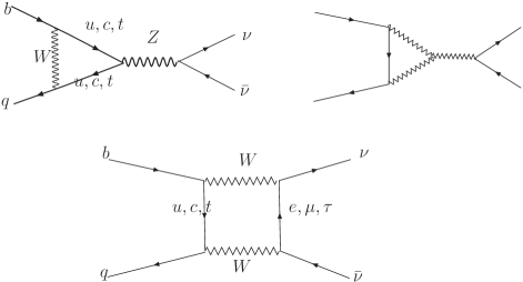
Figure 1: Leading order Feynman diagrams in SM for $b\to q\nu\bar{\nu}$, with $q=s$ or $d$.

$$H=C(\bar{q}\gamma_{\mu}P_{L}b)(\bar{\nu}\gamma^{\mu}P_{L}\nu),$$ (1)

with $P_{L}=(1-\gamma_{5})/{2}$. The coefficient $C$ is

$$C=\frac{\sqrt{2}G_{F}\alpha}{\pi\sin^{2}\theta_{w}}V_{tb}V^{*}_{tq}\frac{x}{8}\left[\frac{x+2}{x-1}+\frac{3x-6}{(x-1)^{2}}\ln{x}\right],$$ (2)

and $x={m_{t}^{2}}/{m_{W}^{2}}$. From this expression, we can see that the coefficient $C$ is sensitive to the mass of the particle in loop. If new particle exist, it should affect the Wilson Coefficient and change the branching ratio. That is why this kind of flavor changing neutral current processes is sensitive to new physics [6].

We have already mentioned that the pure leptonic ($\nu\bar{\nu}$) decay is forbidden due to helicity conservation. However, when a photon is emitted from any charged line of $b$ or $q$ quark, this pure leptonic processes turn into radiative ones and helicity suppression does not exist anymore. At quark level the process $B_{s(d)}\rightarrow\gamma\nu\bar{\nu}$ is described by the same diagrams as $b\rightarrow q\gamma\nu\bar{\nu}$ shown in Fig.2. Incidentally, we should note the following peculiarities of this process:

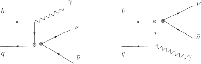
Figure 2: Feynman diagrams for $b\to q\gamma\nu\bar{\nu}$ using effective four fermi operators.

• when photon emitted from internal charged particles (W or top quark), the above mentioned process will be suppressed by a factor ${m_{b}^{2}}/{m_{W}^{2}}$ (see [3]), in comparison to the process $b\to q\nu\bar{\nu}$, one can neglect the contribution of such diagrams.

• The Wilson coefficient $C$ is the same for the processes $b\to q\gamma\nu\bar{\nu}$ and $b\rightarrow q\nu\bar{\nu}$ as a consequence of the extension of the Low’s low energy theorem (for more detail see [11]).

So, when photon emitted from initial $b$ or light quark line, there are only two diagrams, contributing to the process $b\rightarrow q\gamma\nu\bar{\nu}$. From Fig.2, the corresponding decay amplitude turns out to be

$${\cal A}=-\frac{e}{6}C~{}\bar{q}\left[\not\!\epsilon^{*}_{\gamma}\frac{\not\!p_{\gamma}-\not\!p_{q}+m_{q}}{(p_{q}\cdot p_{\gamma})}\gamma_{\mu}P_{L}+P_{R}\gamma_{\mu}\frac{\not\!p_{b}-\not\!p_{\gamma}+m_{b}}{(p_{b}\cdot p_{\gamma})}\not\!\epsilon^{*}_{\gamma}\right]b~{}(\bar{\nu}\gamma^{\mu}P_{L}\nu).$$ (3)

3 Analytical and Numerical results

In order to calculate analytic formulas of the decay amplitude, we use the wave functions $\Phi_{M,\alpha\beta}$ decomposed in terms of spin structure. In the summation procedures, the $B$ meson is treated as a heavy-light system. Thus, the $B$ meson light-cone matrix element can be decomposed as [12]:

$$\Phi_{B,\alpha\beta}=\frac{i}{\sqrt{2N_{c}}}\left\{(\not\!P_{B}\gamma_{5})_{\alpha\beta}\phi_{B}^{A}+\gamma_{5\alpha\beta}\phi_{B}^{P}\right\},$$ (4)

where $N_{c}=3$ is color degree of freedom, $P_{B}$ is the corresponding meson’s momentum, $\phi_{B}^{A}$ and $\phi_{B}^{P}$ are Lorentz scalar distribution amplitudes. As heavy quark effective theory leads to $\phi_{B}^{P}\simeq M_{B}\phi_{B}^{A}$, then $B$ meson’s wave function can be expressed by

$$\Phi_{B,\alpha\beta}(x)=\frac{i}{\sqrt{2N_{c}}}\left[\not\!P_{B}+M_{B}\right]\gamma_{5\alpha\beta}\phi_{B}(x).$$ (5)

In above function, the function $\phi_{B}$ describes the momentum distribution amplitude. Since $b$ quark is much heavier than the light quark in $B$ meson, there is a sharp peak at the small $x$ region for the light quark momentum fraction,

$$\phi_{B}(x)=N_{B}x^{2}(1-x)^{2}\exp\left[-\frac{M_{B}^{2}\ x^{2}}{2\omega_{b}^{2}}\right].$$ (6)

It satisfies the normalization relation:

$$\int_{0}^{1}\phi_{B}(x)dx=\frac{f_{B}}{2\sqrt{2N_{c}}}\;,$$ (7)

with $f_{B}$ the $B$ meson decay constant. This choice of $B$ meson’s wave function is almost a best fit from the $B$ meson non-leptonic two body decays [8].

For simplicity, we consider the B meson at rest and use the light-cone coordinate $(p^{+},p^{-},\vec{p}_{\perp})$ to describe the meson and quark’s momenta, where $p^{\pm}=\frac{1}{\sqrt{2}}(p^{0}\pm p^{3})$ and $p_{\perp}=(p^{1},p^{2})$. Using these coordinate we can take the $B_{q}$, $\nu\bar{\nu}$ (momentum sum) and photon’s momenta as

$$P_{B}=\frac{M_{B}}{\sqrt{2}}(1,1,\vec{0}_{\perp});~{}\ \ ~{}P_{\nu\bar{\nu}}=\frac{M_{B}}{\sqrt{2}}(1,r^{2},\vec{0}_{\perp});~{}\ \ ~{}P_{\gamma}=\frac{M_{B}}{\sqrt{2}}(0,1-r^{2},\vec{0}_{\perp}),$$ (8)

with $r^{2}={P_{\nu\bar{\nu}}^{2}}/{M_{B}^{2}}$. The momenta of $b$ and $q$ quark in B meson are $p_{b}=(1-x)P_{B}$, $p_{q}=xP_{B}$. Using above convention, the amplitude for $B_{q}\to\gamma\nu\bar{\nu}$ decay is written by:

$$A=\frac{\sqrt{6}eC}{6}\left[~{}iC_{1}\epsilon_{\alpha\beta\mu\nu}\varepsilon^{*\alpha}P_{\gamma}^{\beta}P_{B}^{\nu}+C_{2}~{}(P_{\gamma\mu}\varepsilon^{*}_{\nu}-P_{\gamma\nu}\varepsilon^{*}_{\mu})~{}P_{B}^{\nu}\right](\bar{\nu_{1}}\gamma^{\mu}p_{L}\nu_{2})$$ (9)

with

$$C_{1}=\int_{0}^{1}\frac{\Phi(x)}{p_{b}\cdot P_{\gamma}}+\int_{0}^{1}\frac{\Phi(x)}{p_{q}\cdot P_{\gamma}}$$ (10)

$$C_{2}=\int_{0}^{1}\frac{\Phi(x)}{p_{q}\cdot,P_{\gamma}}-\int_{0}^{1}\frac{\phi(x)}{p_{b}\cdot P_{\gamma}}.$$ (11)

After squaring the amplitude and performing the phase space integration over one of the two Dalitz variables, and summing over three generation of neutrinos, we get the differential decay width versus the photon energy $E_{\gamma}$:

$$\frac{d\Gamma}{dE_{\gamma}}=\frac{6C^{2}\alpha}{(12\pi)^{2}}~{}(C_{1}^{\prime 2}+C_{2}^{\prime 2})~{}(M_{B}-2E_{\gamma})E_{\gamma},$$ (12)

with

$$C_{1}^{\prime 2}=\left(\int_{0}^{1}\frac{\Phi(x)}{1-x}dx+\int_{0}^{1}\frac{\Phi(x)}{x}dx\right)^{2}$$ (13)

$$C_{2}^{\prime 2}=\left(\int_{0}^{1}\frac{\Phi(x)}{1-x}dx-\int_{0}^{1}\frac{\Phi(x)}{x}dx\right)^{2}.$$ (14)

By integrating the variable $E_{\gamma}$, we get the decay width:

$$\Gamma=\frac{M_{B}^{3}C^{2}\alpha}{(24\pi)^{2}}(C_{1}^{\prime 2}+C_{2}^{\prime 2}).$$ (15)

In this work, we use following parameters [7, 13]:

$$\omega_{b}=0.4,~{}f_{B}=0.19~{}\mathrm{GeV},~{}\tau_{B^{0}}=1.54\times 10^{-12}s;$$

$$\omega_{b_{s}}=0.5,~{}f_{Bs}=0.24~{}\mathrm{GeV},~{}\tau_{B_{s}}=1.46\times 10^{-12}s;$$

$$G_{F}=1.66\times 10^{-5}\mathrm{GeV}^{-2};~{}\sin^{2}\theta_{\omega}=0.23;~{}\alpha=\frac{1}{132}$$

$$V_{tb}=0.999,~{}~{}V_{td}=0.0074,~{}~{}V_{ts}=0.041.$$ (16)

Using these parameters, we get the branching ratios:

$$\mathbf{Br}(B^{0}\to\gamma\nu\bar{\nu}) = 0.7\times 10^{-9},$$

$$\mathbf{Br}(B_{s}\to\gamma\nu\bar{\nu}) = 2.4\times 10^{-8}.$$ (17)

Just as we mentioned above, many approaches have been used to analyze these processes such as constituent quark model [3], pole model [3, 14], QCD sum rule [4], and light front approach [5]. Here we compare our results with them which is shown in Table. 1.

Table 1: Comparison of results from different approaches

Mode	Our Results	Quark Model	Pole Model	Sum Rule	light front
$\mathbf{BR}(B^{0}\to\gamma\nu\bar{\nu})$	$0.74\times 10^{-9}$	$1.7\times 10^{-9}$	$2.1\times 10^{-9}$	$4.2\times 10^{-9}$	$1.4\times 10^{-9}$
$\mathbf{BR}(B_{s}\to\gamma\nu\bar{\nu})$	$2.4\times 10^{-8}$	$3.5\times 10^{-8}$	$1.8\times 10^{-8}$	$7.5\times 10^{-8}$	$2.0\times 10^{-8}$

In constituent quark model, the non-relativity character is considered. If we replace our $B$ meson distribution amplitude in eq.(6) by a $\delta$ function $({f_{B}}/{2\sqrt{6}})~{}\delta(x-m_{q}/m_{B})$, our formula will return back to the constituent quark model in ref.[3]. Since we have poor knowledge about quark mass up to now, our new calculation is surely an improvement. In paper [3], the authors also calculate these processes in the pole model, and the results are similar to the quark model case. From the table, one can also see that most of the methods get similar results except the QCD sum rule approach, whose result is larger than others. We hope the experiments in future can test these different methods.

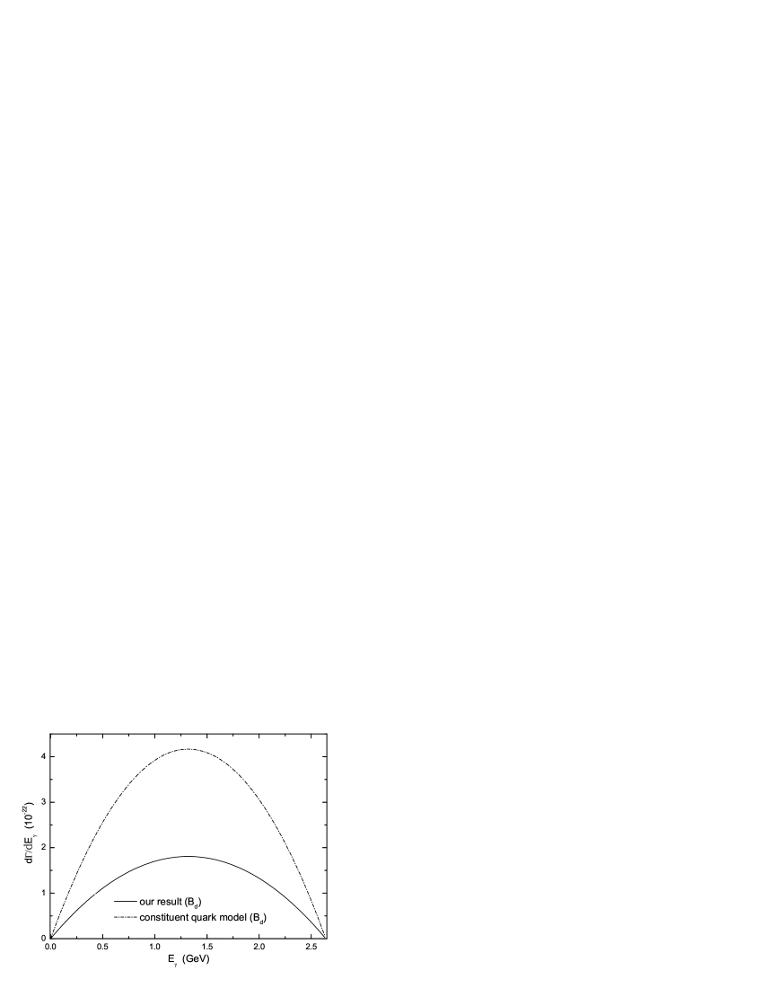
Figure 3: Differential decay rate of $B^{0}\to\gamma\nu\bar{\nu}$ versus the photon energy $E_{\gamma}$.

In Fig. (3) and Fig. (4), we figure out the differential decay rate of $B^{0}(B_{S})\to\gamma\nu\bar{\nu}$ versus photon energy $E_{\gamma}$. We also display the photon energy spectrum from constituent quark model. From these figures, we find our results are smaller than the constituent quark one, but the shape of the spectrum is the same. If normalized decay rate is used, the two lines will become only one, since the function is very simple

$$f(x)=24x(1-2x)$$ (18)

which can be extracted from eq.(12).

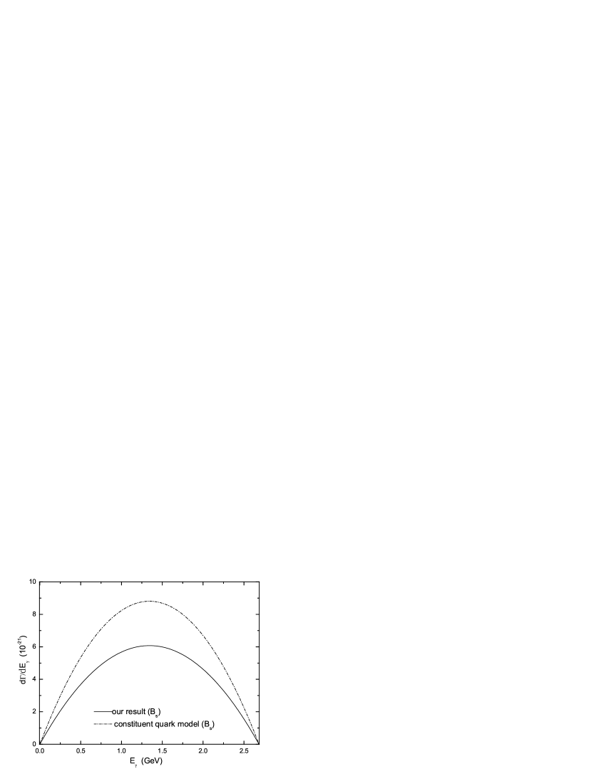
Figure 4: Differential decay rate of $B_{s}\to\gamma\nu\bar{\nu}$ versus the photon energy $E_{\gamma}$.

Of course, there are also uncertainties in our calculation. The most large uncertainty comes from the heavy meson wave function. The high order twists contribution, the high Fock states are also not included, because they are not clear completely now. We hope that the non-leptonic $B$ meson decay can offer more information in the near future.

4 Summary

In this work, we calculate the branching ratios in SM for $B_{s}\to\gamma\nu\bar{\nu}$ to be $10^{-8}$ and for $B^{0}\to\gamma\nu\bar{\nu}$ to be $10^{-9}$ using $B$ meson wave function constrained from non-leptonic B decays. These decay channels are useful to determine the decay constants $f_{B}$ and wave function. After calculation, we find our leading order results are at the same order as other approaches but a little smaller. These rare decays are sensitive to any new physics contributions which can be measured by future experiment such as LHCb.

References

• [1] B.A. Campbell and P.J. O’Donnell, Phys. Rev. D25 (1982) 1989;
A. Ali, B decays, ed. S. Stone (World Scientific, Singapore) p.67.
• [2] Z. Ligeti and M.B. Wise, Phys. Rev. D53, 4937 (1996).
• [3] C.-D. LΓΌ, D.-X. zhang, Phys. lett. B 381 (1996) 348.
• [4] T. M. Aliev, A. Ozpineci, M. Savci, Phys. Lett. B393 (1997) 143.
• [5] C.-Q. Geng, C.-C. Lih, W.-M Zhang, Phys. Rev. D 57 (1998) 5697.
• [6] B. Sirvanli, G. Turan, Mod. Phys. Lett. A 18 (2003) 47.
• [7] H.-N Li, B. Melic, Eur. Phys. J. C 11 (1999) 695;
T. Huang, X.-G Wu, Phys. Rev. D71 (2005) 034018.
• [8] H.-N. Li, H.-L. Yu, Phys. Rev. D53 (1996) 2480;
Y.-Y. Keum, H.-N. Li, A.I. Sanda, Phys. Rev. D63 (2001) 054008 ;
C.-D. Lu, K. Ukai, M.-Z. Yang, Phys. Rev. D63 (2001) 074009.
• [9] Y.-Y. Charng, H.-N. Li, Phys. Rev. D72 (2005) 014003.
• [10] T. Inami and C.S. Lim, Prog. Theor. Phys. 65 (1981) 297; 65 (1982) 1772 (E);
G. Buchalla, A. J. Buras, Nucl. Phys. B400 (1993) 225.
• [11] G. L. Lin, J. Liu and Y. P. Yao, Phys. Rev. D42 (1990) 2314.
• [12] A.G. Grozin, M. Neubert, Phys. Rev. D55, 272 (1997);
M. Beneke, T. Feldmann, Nucl. Phys. B592, 3 (2001);
M. Beneke, G. Buchalla, M. Neubert, C.T. Sachrajda, Nucl. Phys. B591, 313 (2000).
• [13] Particle Data Group, S. Eidelman, et al., Phys. Lett. B 592, 1 (2004).
• [14] H.-Y. Cheng, et al.,Phys. Rev. D51 (1995) 1199.