Signatures of anomalous interactions at a linear collider
Abstract
We examine, in a model independent way, the sensitivity of a Linear Collider to the couplings of a light Higgs boson to gauge bosons. Including the possibility of violation, we construct several observables that probe the different anomalous couplings possible. For an intermediate mass Higgs, a collider operating at a center of mass energy of 500 GeV and with an integrated luminosity of 500 fb-1 is shown to be able to constrain the vertex at the few per cent level, and with even higher sensitivity in certain directions. However, the lack of sufficient number of observables as well as contamination from the vertex limits the precision with which the coupling can be measured.
pacs:
14.80.Cp, 14.70.FM, 14.70.HpI Introduction
Although the standard model (SM) has withstood all possible experimental challenges and has been tested to an unprecedented degree of accuracy, so far there has been no direct experimental verification of the phenomenon of spontaneous symmetry breaking. With the latter being considered a central pillar of this theory and its various extensions, the search for a Higgs boson is one of the main aims for many current and future colliders Godbole:2002mt . Within the SM, the only fundamental spin- object is the (-even) Higgs boson and remains the only particle in the SM spectrum to be found yet. Rather, a lower bound on the mass of the SM Higgs boson, (about 114.5 GeV) is provided by the direct searches at the LEP collider higmin . Electroweak precision measurements, on the other hand, provide an upper bound on its mass of about 204 GeV at 95% C.L. higmax . It should be realized that both these limits are model dependent and may be relaxed in extensions of the SM. For example, the lower limit can be relaxed in generic 2-Higgs doublet models 2hdm or in models with violation cp-mssm . In the latter case, direct searches at LEP and elsewhere still allow the lightest Higgs boson to be as light as 10 GeV lowerH . Similarly, the upper bound on the mass of the (lightest) Higgs in some extensions may be substantially higher highH . The Large Hadron Collider (LHC) is expected to be capable lhc-tdr of searching for the Higgs boson in the entire mass range allowed.
It is then quite obvious that just the discovery of the Higgs boson at the LHC will not be sufficient to validate the minimal SM. For one, the only neutral scalar in the SM is a state arising from a doublet with hypercharge 1, while its various extensions can have several Higgs bosons with different properties and quantum numbers. The minimal supersymmetric standard model (MSSM), for example, has two -even states and a single -odd one rmg . Thus, should a neutral spin-0 state be observed at the LHC, a study of its -property would be essential to establish it as the SM Higgs boson godbole .
Since, at an collider, the dominant production modes of a neutral Higgs boson proceed via its coupling with a pair of gauge bosons (), any change in the couplings from their SM values can be probed via such production processes. Within the SM/MSSM, the only (renormalizable) interaction term involving the Higgs boson and a pair of gauge bosons is the one arising from the Higgs kinetic term. However, once we accept the SM to be only an effective low-energy description, higher-dimensional (and hence non-renormalizable) terms are allowed. If we only demand Lorentz invariance and gauge invariance, the most general coupling structure may be expressed as
| (1) | |||||
where denote the momenta of the two ’s (’s), and . In the context of the SM, at the tree level, while the other couplings vanish identically. At the one-loop level or in a different theory, effective or otherwise, these may assume significantly different values. We study this most general set of anomalous couplings of the Higgs boson to a pair of s and at a linear collider (LC) in the processes , with being a light fermion.
The various kinematical distributions for the process , proceeding via vector boson fusion and Higgsstrahlung, with unpolarized beams has been studied in the context of the SM dist . The effect of beam polarization has also been investigated for the SM pol . The anomalous couplings have been studied in Refs.rattazzi ; stong ; He:2002qi ; Hagiwara:1993ck ; Gounaris:1995mx for the LC and in Refs.Zhang:2003it ; plehn for the LHC in terms of higher dimensional operators. Ref. Hagiwara:2000tk investigates the possibility to probe the anomalous couplings, , using the optimal observable technique oot for both polarized and un-polarized beams. Ref. t.han , on the other hand, probes the -violating coupling by means of asymmetries in kinematical distributions and beam polarization. In Ref. maria , the vertex is studied in the process of using angular distributions of the decay products.
The rest of the paper is organized as follows. In section II we discuss the possible sources and symmetries of the anomalous couplings and the rates of various processes involving these couplings. In section III we construct several observables with appropriate and property to probe various anomalous couplings. In section IV we construct similar observables to probe anomalous couplings, which we then use along with the ones constructed for the case. Section V contains a discussion and summary of our findings.
II The couplings
The anomalous couplings in Eq.(1) can appear from various sources such as via higher order corrections to the vertex in a renormalizable theory kniehl:NPB or from higher dimensional operators in an effective theory operator . For example, in the MSSM, the non-zero phases of the trilinear SUSY breaking parameter and the gaugino/higgsino mass parameters can induce -violating terms in the scalar potential at one loop level even though the tree level potential is -conserving. As a consequence, the Higgs-boson mass eigenstates can turn out to be linear combinations of -even and -odd states. This modifies the effective coupling of the Higgs boson to the known particles from what is predicted in the SM (or even from that within a version of MSSM with no -violation accruing from the scalar sector).
In a generic multi-doublet model, whether supersymmetric sumrule or otherwise Choudhury:2003ut , the couplings of the neutral Higgs bosons to a pair of gauge bosons satisfy the sum rule
Thus, while for a given Higgs boson can be significantly smaller than the SM value, any violation of the above sum rule would indicate either the presence of higher multiplets or more complicated symmetry breaking structures (such as those within higher-dimensional theories) Choudhury:2003ut . The couplings or can arise only at a higher order in a renormalizable theory kniehl:NPB . Furthermore, within models such as the SM/MSSM where the tree-level scalar potential is -conserving, may be generated only at an order of perturbation theory higher than that in which the Higgs sector acquires -violating terms. However, in an effective theory, which satisfies symmetry, the couplings and can arise, at the lowest order, from terms such as or operator where is the usual Higgs doublet, is a field strength tensor and its dual. It can be easily ascertained that the effects of the higher dimensional terms in the trilinear vertices of interest can be absorbed into () by ascribing them with non-trivial momentum-dependences (form factor behavior). Clearly, if the cut-off scale of this theory is much larger than the typical energy at which a scattering experiment is to be performed, the said dependence would be weak. In all processes that we shall be considering, this turns out to be the case. In particular, the Bjorken process (Fig. 1(b)) essentially proceeds at a fixed center-of-mass energy, hence both and are constant for this process. Even for the other processes of interest, namely gauge boson fusion (Fig. 1(a)), the momentum dependence of the form-factors have a rather minor role to play, especially for . This suggests that we can treat as phenomenological and energy-independent parameters.
II.1 Symmetries of anomalous couplings
A consequence of imposing an symmetry would be to relate the anomalous couplings, and , for the vertex with those for the vertex. However, rather than attempting to calculate these couplings within a given model, we shall treat them as purely phenomenological inputs, whose effect on the kinematics of various final states in collider processes can be analyzed.
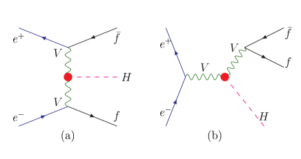
In general, each of these couplings can be complex, reflecting possible absorptive parts of the loops, either from the SM or from some new high scale physics beyond the SM. It is easy to see that a non-vanishing value for either or destroys the hermiticity of the effective theory. Such couplings can be envisaged when one goes beyond the Born approximation, whence they arise from final state interactions, or, in other words, out of the absorptive part(s) of higher order diagrams, presumably mediated by new physics. A fallout of non-hermitian transition matrices is non-zero expectation values of observables which are odd under , where stands for the pseudo-time reversal transformation, one which reverses particle momenta and spins but does not interchange initial and final states. Of course, such non-zero expectation values will be indicative of final state interaction only when kinematic cuts are such that the phase space integration respects . Note that too can be complex in general and can give an additional -odd contribution. However, for the processes that we will consider, the phase of at least one of and can always be rotated away, and we make this choice for . Henceforth, we shall assume that and are close to their SM value, i.e. , the rationale being that any departure from and respectively would be the easiest to measure
Unfortunately, this still leaves us with many free parameters making an analysis cumbersome. One might argue that gauge invariance would predict . However, once symmetry breaking effects are considered, this does not necessarily follow kniehl:NPB . Nevertheless, we will make this simplifying assumption that is real and equal to , i.e. , since the equality is found to hold true in some specific cases awaz (and would be dictated if were to be an exact symmetry of the effective theory). With this assumption, we list, in Table 1, the and properties of such operators.
| Trans. | |||||
|---|---|---|---|---|---|
Finally, keeping in view the higher-dimensional nature of all of these couplings, we retain only contributions up to the lowest non-trivial order, arising from terms linear in the additional couplings.
II.2 Cross-sections
The dominant channels of Higgs production at an electron-positron colliders are
-
1.
the 2-body Bjorken process ();
-
2.
in association with a pair of neutrinos (), i.e. -fusion;
-
3.
in association with an pair (), i.e. -fusion
Note that the Bjorken-process also contributes to the other two final states through the subsequent decay of the . Of these three, the channel is considerably suppressed (by almost a factor of 10) with respect to the channel over a very wide range of center-of-mass energies () and Higgs masses. As can be expected, at large , the Bjorken process suffers the usual -channel suppression and has a smaller cross section compared to that for -fusion. In fact, even for and unpolarized beams, the Bjorken process dominates over -fusion only for relatively large Higgs masses Djouadi:2005gi ; Barger:1993wt ; Choudhury:2002qb .
In view of this, it might seem useful to concentrate first on the dominant channel, viz and thereby constrain and . However, it is immediately obvious that the Bjorken process too contributes to this final state and hence the couplings , and have a role to play. Since the total rate is a -even (as well as even) observable, it can receive contribution only from . [Note that a non-zero would only rescale the SM rates.] The other non-standard couplings, odd under and/or , are responsible for various polar and azimuthal asymmetries and contribute nothing to the total rate on integration over a symmetric phase space555Remember that we work only to the linear order in the anomalous couplings. Thus they contribute only through the interference terms with the SM amplitude.. This can be understood best by considering the square of the invariant amplitude pertaining to on-shell -production, namely :
| (2) |
with denoting the electron’s couplings to the , and the energy, momentum and scattering angle of the in the c.m.-frame. The proportionality constant includes, alongwith the couplings etc., a factor . This suggests that the anomalous contribution vanishes for large , inspite of the higher-dimensional nature of the coupling. Furthermore, Eq.(2) also demonstrates that neither nor may make their presence felt if the polarization of the could simply be summed over. It also shows that the contribution due to would disappear when integrated over a symmetric part of the phase space as has been mentioned before. Thus, if we want to probe these couplings, we would need to look at rates integrated only over partial (non-symmetric) phase space. As an example, let us consider the forward-backward asymmetry for the -boson. As can be seen from Eq.(2), it is proportional to alone. This can be understood by realizing that this observable is proportional to the expectation value of and hence is a -odd and -even quantity just as is. For and , which are -odd, one has to look at the azimuthal correlations of the final state fermions. Equivalently one can look for partial cross-section, restricting the azimuthal angles over a given range. A discussion of how partial cross-section can be used to probe anomalous couplings is given in Appendix A. Further, Eq.(2) also indicates that the angular distribution of the Higgs (or, equivalently, that of the ) is different for the SM piece than that for the piece proportional to ; the difference getting accentuated at higher . This, in principle, could be exploited to increase the sensitivity to .
In this paper we restrict ourselves to the case of a first generation linear collider. For such , the interference between the -fusion diagram with the -channel one is enhanced for non-zero and . At a first glance, it may seem that the kinematic difference between the two set of diagrams could be exploited and the two contributions separated from each other with some simple cuts. However, in actuality, such a simple approach does not suffice to adequately decouple them. It is thus contingent upon us to first constrain the non-standard couplings from processes that involve just these and only then to attempt to use -fusion process to probe the vertex.
III The couplings
The anomalous couplings have been studied earlier in the process in the presence of an anomalous coupling Hagiwara:2000tk making use of optimal observables oot . The -violating anomalous couplings alone have also been studied in Ref. t.han , which constructs asymmetries for both polarized and unpolarized beams. We, however, choose to be conservative and restrict ourselves to unpolarized beams. And, rather than advocating the use of complicated statistical methods, we construct various simple observables that essentially require only counting experiments. Furthermore, we include the decay of the Higgs boson, account for -tagging efficiencies and kinematical cuts to obtain more realistic sensitivity limits. Since we are primarily interested in the intermediate mass Higgs boson ( GeV), is the dominant decay mode with a branching fraction .
III.1 Kinematical Cuts
For a realistic study of the process , we choose to work with a Higgs boson of mass 120 GeV and a collider center-of-mass energy of 500 GeV. To ensure detectability of the -jets, we require, for each, a minimum energy and a minimum angular deviation from the beam pipe. Furthermore, the two jets should be well separated so as to be recognizable as different ones. To be quantitative, we require that
| (3) |
where with and denoting the separation between the two -jets in azimuthal angle and rapidity respectively.
For events with the decaying into a pair of leptons or light quarks, we have similar demands on the latter, namely
| (4) |
For leptons, i.e. , we require a lepton–lepton separation:
| (5) |
along with a jet–lepton isolation:
| (6) |
for each of the four jet-lepton pairings. For , i.e. light quarks, we impose, instead,
| (7) |
for each of the six pairings. On the other hand, if the were to decay into neutrinos, the requirements of Eqs.(4–7) are no longer applicable and instead we demand that the events contain only the two -jets along with a minimum missing transverse momentum, viz
| (8) |
The above set of cuts select the events corresponding to the process of interest, rejecting most of the QED-driven backgrounds. To further distinguish between the role of the Bjorken diagram and that due to the () fusion in the case of () final state we need to select/de-select the events corresponding to the -mass pole. This is done via an additional cut on the invariant mass of , viz.
| (9) |
Since an exercise such as the current one would be undertaken only after the Higgs has been discovered and its mass measured to a reasonable accuracy, one may alternatively demand that the energy of the Higgs (reconstructed pair) is close to , namely
| (10) |
where . This has the advantage of being applicable to the final state as well. The -jet tagging efficiency is taken to be 0.7. We add the statistical error and a presumed 1% systematic error (accruing from luminosity measurements etc.) in quadrature. In other words, the fluctuation in the measurement of a cross-sections is assumed to be
| (11) |
while that for an asymmetry is
| (12) |
Here is the SM value of cross-section, is the integrated luminosity of the collider and is the fractional systematic error. Since we work in the linear approximation for the anomalous couplings, any observable, rate or asymmetry, can be written as
Then we define the blind region as the region in the parameter space for which
| (13) |
where is the degree of statistical significance, is the SM value of and is the statistical fluctuation in . All the limits and blind regions quoted in this paper are obtained using the above relation. Note that in all the cases that we will consider, the asymmetries vanish identically within the SM.
III.2 Cross-sections
The simplest observable, of course, is the total rate. Note that , inspite of being -odd, does result in a non-zero, though small, contribution to the total cross-section. This is but a consequence of the absorptive part in the propagator and would have been identically zero in the limit of vanishing widths. Since we retain contributions to the cross-section that are at best linear in the couplings, the major non-trivial anomalous contribution, on imposition of the cut, emanates from with only subsidiary contributions from . For our default choice (a 120 GeV Higgs at a machine operating at ), on selecting the -pole ( cut) the rates, in femtobarns, are
| (14) |
On de-selecting the -pole ( cut) we obtain, instead
| (15) |
The total rates, by themselves, may be used to put stringent constraints on . For decaying into light quarks and s (with the cut) and for an integrated luminosity of , the lack of any deviation from the SM expectations would give
| (16) |
at the level. We do not use the final state in deriving the above constraint as it receives a contribution proportional to too. This arises from the interference of the Bjorken diagram with the -fusion diagram due to the presence of the absorptive part in the near-on-shell -propagator.
The cross-sections shown in Eqs.(14 & 15) and the constraint of Eq.(16) have been derived assuming the SM value for . Clearly, any variation in would affect the total rates and thus it is interesting to investigate possible correlations between and . Parameterizing small variations in as , the cross-sections can be re-expressed as
| (17) |
and
| (18) |
where stands for cross-section with cut with and light quarks in the final state, i.e., the combination used to obtain Eq.(16), and, as before, terms quadratic in small parameters have been neglected. Using these two rates we can obtain simultaneous constraints in the plane, as exhibited in Fig. 2. The oblique lines are obtained using Eq.(17) whereas the almost vertical lines are obtained using Eq.(18). Thus, alone can constrain to within a few percent of the SM value. It is amusing to consider, at this stage, the possibility that could have been large, as for example happens in the MSSM. Clearly, the very form of Eqs.(17 & 18) tells us that this would have amounted to just a two-fold ambiguity with a second and symmetric allowed region lying around . Since we are interested in the SM like Higgs boson, we constrain ourselves to region near as shown in Fig. 2.
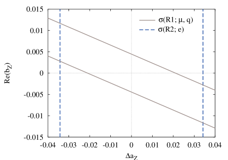
From Eq.(14) and Eq.(17) it is clear that the total rates, for the cut, depend on only one combination of and , i.e. on
| (19) |
With this combination we can write all the cross-sections given in Eqs.(14) and (17) as , where the limit from Fig. 2 translates to
| (20) |
i.e., % () variation of the rates. This variation can also be parameterized with keeping or with keeping , (i.e., the intercepts of the solid lines in Fig. 2 on the – and –axes respectively). In other words, the individual limit, i.e. the limit obtained keeping only one anomalous coupling non-zero, on is 0.0044 and that on is 0.021. On the other hand, if the cut were to be operative, we obtain the constraint almost independent of , see Fig. 2. This constraint translates to a % () variation in the rate .
Note that the contributions proportional to the absorptive part of the -propagator are proportional to away from the resonance, i.e. for the cut. Hence in this case it is a higher order effect and thus ignored in Eqs.(15) and (18). On the other hand, near the -resonance these terms are proportional to and hence of the same order in the perturbation theory. Thus, in order to be consistent at a given order in the coupling we retain these contribution only with the cut.
III.3 Forward-backward asymmetry
The final state constitutes of two pairs of identifiable particles : coming from the decay of Higgs boson and , where . One can define forward-backward asymmetry with respect to all the four fermions. But we choose, among them, the asymmetries with definite transformation properties under and . In the present case we have only one such forward-backward asymmetry, i.e. the expectation value of . In other words, it is the forward-backward asymmetry with respect to the polar angle of the Higgs boson (up to an overall sign) and given as
| (21) |
This observable is odd and even, and hence a probe purely of of [see Table 1]. Note that this asymmetry is proportional to , where are the right-(left-) handed couplings of the electron to the -boson. With the cut—see Eq.(9)—operative, a semi-analytical expression for this asymmetry, keeping only terms linear in the anomalous couplings, is given by
| (22) |
In the above, “” stands for all four flavors of light quarks summed over and . Note here, that the contribution to the denominator of Eq.(21) from the anomalous terms have been dropped as the formalism allows us to retain terms only upto the first order in these couplings. In any case, their presence would have had only a miniscule effect on the ensuing bounds. The asymmetry corresponding to the cut is very small and is not considered. Omitting the () final state on account of the presence of , we use only the light quarks and s. For an integrated luminosity of 500 fb-1, the corresponding limit is
| (23) |
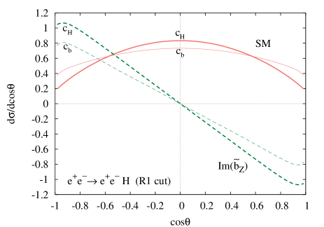
It is interesting to speculate as to the sensitivity of the a forward-backward asymmetry constructed with respect to the angle subtended by, say, the -jet, rather than that for the reconstructed . Since the quarks are spherically distributed in the rest frame of Higgs, their angular distributions track that of the Higgs boson, modulo some smearing [see Fig. 3]. This is as true for the anomalous contribution as for the SM. The smearing only serves to decrease the sensitivity as is evinced by the forward-backward asymmetries constructed with respect to , the polar angle of the quark. For events corresponding to the cut, this amounts to
Using final states with s or light quarks, one may then use to probe down to
at level, for an integrated luminosity of 500 fb-1, and assuming all the other anomalous couplings to be zero. It is not surprising that the sensitivity is lower as compared to that of —see Eq.23—for carries only subsidiary information leading to a reduction in the size of the asymmetry. Put differently, the distribution for the is identical to that for the (thereby eliminating the need for charge measurement) and each is driven primarily by .
Note that we have desisted from using the non-zero forward-backward asymmetry in the polar angle distribution of . Such observables do not have the requisite -properties and are, in fact, non-zero even within the SM. The presence of non-zero provides only an additional source for the same and the limits extractable would be weaker than those we have obtained.
III.4 Up-down asymmetry
The Higgs being a spin–0 object, its decay products are isotropically distributed in its rest frame. This, however, is not true of the . Still, conservation ensures that the leptons from decay are symmetrically distributed about the plane of production. Thus, an up-down asymmetry defined as
| (24) |
can be non-zero for the anomalous couplings. In other words, a non-zero expectation value for is a odd (and odd) observable. In our notation, it is driven by the non-zero real part of , and, for our choice of parameters, amounts to
| (25) |
up to linear order in the anomalous couplings. In obtaining Eq.25, the cut has been imposed on the invariant mass. Note that, except for the final state, is a probe purely of . The cross section for the final state receives additional contribution from due to the absorptive part of the -propagator in the Bjorken diagram. Although and offer much larger sensitivity to than do either of and , the former can not be used as the measurement of such asymmetries requires charge determination for light quark jets. However, one can determine the charge of -quarks b-charge and using , for the ’s resulting from the decay, we may obtain, for an integrated luminosity of 500 fb-1, a bound of
with 100% charge determination efficiency and only
if the efficiency were 20%. Note though that the final state is beset with additional experimental complications (such as final state combinatorics) than the semileptonic channels and hence we would not consider this in deriving our final limits. Note that we do not account for any combinatorics in obtaining the above said limits. However, we argue that the invariant masses of the pair coming from and are non-overlapping hence the change in the above limits due to combinatorics are expected to be small.
Another obvious observable is . Using this, an integrated luminosity of 500 fb-1, would lead to a constraint of
| (26) |
The reduced sensitivity of the channel as compared to the channel is easy to understand. As Eq.(48) demonstrates, . Since , this naturally leads to an additional suppression for .
For the case, on the other hand, the -fusion diagram leads to a contribution that is proportional to and is, thus, unsuppressed. Accentuating this contribution by employing the cut on , we have
| (27) |
and this, for an integrated luminosity of 500 fb-1, leads to a constraint of
| (28) |
Here we note that the limit on , obtained using the cut given above, is much better than the one obtained using cut in Eq.(26), or even the one derived from the final state assuming a charge detection efficiency.
III.5 Combined polar and azimuthal asymmetries
Rather than considering individual asymmetries involving the (partially integrated) distributions in either of the polar or the azimuthal angle, one may attempt to combine the information in order to potentially enhance the sensitivity. To this end, we define a momentum correlation of the form
| (29) | |||||
where the sign of the term in the first square bracket decides if the is in forward() hemisphere with respect to the direction of or backward(). Similarly, the sign of the term in second square bracket defines if is above() or below() the Higgs production plane. Thus the expectation value of the sign of this correlation is same as the combined polar-azimuthal asymmetry given by,
| (30) | |||||
with the second equality being applicable for the cut. In the above, is the partial cross-sections for in the forward-up direction and so on for others. Note that is -odd but does not have a definite and hence depends on both the -odd couplings as seen in Eq.(30). We do not consider the analogous asymmetry for final state as it demands charge determination for light quarks (although may be considered profitably). Similarly, for the final state, receives contributions from -even couplings as well and hence not considered for the analysis.
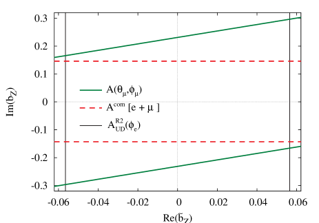
Using this -odd asymmetry along with , and can be constrained simultaneously. Fig. 4 shows the limit on as a function of .
III.6 Another asymmetry
Similar to the previous subsection, we can define a -even and -odd correlation as
| (31) | |||||
which is a probe of the -even and -odd coupling . Here, the sign of the term in the first square bracket decides whether the Higgs boson is in the forward() or backward() hemisphere, while the sign of the term in the second square bracket indicates if is above() or below() the Higgs production plane. The expectation value of the sign of can thus be expressed as an asymmetry of the form
| (32) |
The semi-analytical expression for this asymmetry for cut is given by
| (33) | |||||
Using final states with either electrons or muons, we would obtain a limit of
| (34) |
for 500 fb-1 of integrated luminosity and maintaining all the other form-factors to be zero. This limit is better than the one obtained in the preceding subsection.
Once again, inclusion of the channel, i.e. a measurement of , would improve the situation dramatically even for a nominal charge detection efficiency. For example, an efficiency as low as just 20%, is enough to obtain
We reemphasize though that our final results do not exploit this possibility.
We also note that the sensitivity to the -odd couplings is large for as compare to . As the expressions in the Appendix B demonstrate, , with the cut operational, is proportional to and is proportional to . Thus, for , the asymmetries are proportional to at least one power of where and hence are smaller compared to those for the case.
III.7 Summary of Limits on the couplings
In the preceding five subsections we discussed observables which will be able to probe each of the five anomalous couplings. The ensuing limits are summarized in Table 2.
| Coupling | Bound | Observable used |
|---|---|---|
| with cut; | ||
| with cut; | ||
| with cut; | ||
| with cut | ||
| with cut; | ||
Several points are in order here
-
•
Recall that, of the five anomalous terms, only two viz and , have identical transformations under both and . Consequently, the contributions proportional to the two are intertwined and can only be partially separated. In fact, the most general limits on these two are to be obtained from Fig. 2.
-
•
As for the other three couplings, we have been able to construct observables that are sensitive to only a single coupling, thereby disengaging each of the corresponding bounds in Table 2 from contaminations from any of the other couplings.
-
•
The polar-azimuthal asymmetry, , is sensitive to -odd couplings. However, the limits obtained using final state alone are weaker than the ones obtained by combining and (see Fig 4). Inclusion of electrons in the final state will improve the sensitivity of , but only at the cost of contamination by the -even couplings. Thus, in our present analysis, the role of is only a confirmatory one.
-
•
Note, however, that many of these asymmetries are proportional to . Since this parameter is known to receive large radiative corrections, the importance of calculating higher-order effects cannot but be under-emphasized.
-
•
Observables constraining -odd couplings required charge determination of fermion in the final state thereby eliminating (the dominant) final states from the analysis. This explains a relatively poor limit on . For , the process involves couplings as well. This is discussed in the next section.
IV The couplings
As discussed at the beginning of the last section, the contribution from non-standard couplings to the final state is not negligible even if on-shell production is disallowed by imposing the aforementioned cut. With the neutrinos being invisible, we are left with only two observables: the total cross-section and the forward-backward asymmetry with respect to the polar angle of the Higgs boson. The deviation from the SM expectations for the cross section depends mainly on and . Similarly, the forward-backward asymmetry can be parameterized, in the large, by just . The contribution of the other couplings, viz. and , to either of these observables are proportional to the absorptive part of -propagator and are understandably suppressed, especially for the cut.
Now, irrespective of the properties of the Higgs, its decay products are always symmetrically distributed in its rest frame. In addition, the momentum of the individual neutrino is not available for the construction of any odd asymmetry. Consequently, we do not have a direct probe of and , i.e. the odd couplings.
The event selection criteria we use are the same as in previous section except that the cuts of Eqs. (4 & 6) are replaced by that of Eq. (8). Imposing as argued for earlier, the resultant cross-section, for the cut, can be parameterized as,
| (35) | |||||
while the cut would lead to
| (36) | |||||
Note here that the same as defined in Eq.(19) appears above owing to the assumption . As the contributions proportional to appear due to interference of the fusion diagram with the absorptive part of the -propagator in Bjorken diagram, formally, these terms are at one order of perturbation higher than the rest. Note that the bounds in Table 2 imply that
and hence the corresponding contribution to is at the per-mille level. Since we are not sensitive to such small contributions, we may safely ignore this combination for all further analysis. Looking at fluctuations in , the bound would, then, be
| (37) |
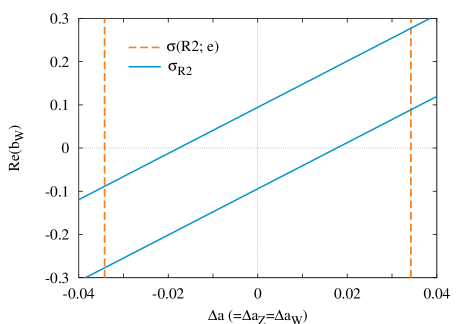
The limits on and are thus strongly correlated and displayed in Fig.5. Note that a complementary bound on had already been obtained in Section III.2. If we assume that, of these two couplings, only one is non-zero, the corresponding individual limits would be (if ) and, similarly, (if ). Interestingly, the last mentioned bound is twice as strong as that obtained in Section III.2. Of course, had we not made the assumption of , or made a different assumption, the bounds derived above (and Fig.5) would have looked very different.
Having constrained , we may now use to investigate possible bounds on . To this end, it is useful to define a further subsidiary variable as
| (38) |
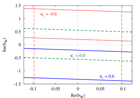
with the inequality having been derived using Table 2. The corresponding constraint in the – plane is shown in Fig. 6 for various representative values of . Clearly, the contamination from the couplings is very large and inescapable. Any precise measurement of , in the present case, requires very accurate determination of the vertex. The individual limit on , for is given in Table 3.
Next, we look at the forward-backward asymmetry with respect to which, for our cuts, we find to be
| (39) | |||||
for the cut, while for the cut it is
| (40) |
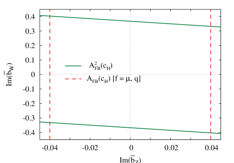
Clearly is the one that is more sensitive to . Once again, there is a strong correlation with , which of course has already been constrained (in Section III.3) from a consideration of similar forward-backward asymmetries in the and channels. The resultant constraint in the – plane is displayed in Fig. 7. And assuming a vanishing , the individual limit on is 0.37.
| Coupling | Limit | Observable used | |
|---|---|---|---|
The only coupling that remains to be constrained at this stage is . While does depend on this parameter, it, unfortunately, also depends on the other three -odd anomalous coupling as well. However, since the lack of sufficient kinematic variables prevent us from constructing another -odd observables, we are forced to use alone, despite its low sensitivity to . Collecting all the relevant vertex dependence into one variable by defining
| (41) |
we have
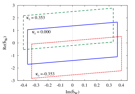
The inequality is a consequence of the bounds derived in the previous section (see Table.2). In Fig. 8, we show the limit on as a function of for three representative values of , namely . The most general limit on can then be gleaned from this figure.
| Coupling | |||
|---|---|---|---|
| – | 0.034 | ||
| 0.097 | 0.28 | ||
| 1.4 | 1.4 | ||
| 2.8 | 2.8 | ||
| 0.40 | 0.40 |
Note that, unlike in the case of the couplings, we have largely been unable to construct observables that are primarily dependent only on a given anomalous coupling. In other words, the constraints are correlated. Thus, it is of interest to obtain the maximal size that these couplings may assume with the aid of such correlations. Such an analysis may be performed by examining the 9-dimensional parameter space (i.e., both and couplings) and delineating the part that would be consistent with all the observables to a given level of confidence. Clearly, the lack of correlations for the couplings renders the blind region to be trivial in five of the nine dimensions and the extent of these remain the same as in Table 2. The most general simultaneous limits on the anomalous couplings obtained using this method are presented in Table 4 for both and . For the -even couplings, such limits are comparable to the corresponding individual limits (Table 3) with only a small dilution due to contamination from vertex. For the -odd couplings, however, the lack of any -odd observable results in a possibly large contamination from vertex. Consequently, the limits on and are only “indirect” and hence poor. Finally, the effect of a non-zero is seen only in due to the large correlation between them (see Fig. 5).
V Discussions
We have constructed observables which, due to their and transformation properties, receive contributions only from specific anomalous couplings with matching and properties. Thus, most of the observables we construct are sensitive only to a single anomalous coupling. This one-to-one correspondence between the observable and the anomalous coupling allows us to obtain a robust constraint on the latter, independent of the values of all the other anomalous couplings. Thus we see from Tables 2 – 4 that the individual and simultaneous limits are the same (or very similar) in most cases. The observables we construct are also very simple from the point of view of experimental measurements. In other words, they are both very physical and easily implementable in actual experiments.
It should also be noted that the limits that we quote on the anomalous couplings, other than those on , are obtained using only asymmetries. In general, asymmetries are more robust with respect to the effects of radiative corrections, except in situations where the tree level contributions are accidentally small. This also means that we have a clear indication as to which observables bear a tighter scrutiny while assessing the effect of radiative corrections. Available calculations of higher order corrections, in the SM rad:sm , to the processes under consideration show that the total rates receive a correction less than 3% for a Higgs with mass about 120 GeV, thus validating our choice of . Since radiative corrections to the processes we consider have been computed not only in the SM rad:sm but also for the MSSM rad:mssm , assessing the effects of these on the rates and asymmetries and hence on the sensitivity for the anomalous couplings will be the next logical step of this analysis which has shown efficacy of these variables to probe these couplings.
Furthermore, in our analysis, we have imposed simple cuts on the kinematic variables which virtually eliminate the non-Higgs backgrounds to the particular final states under consideration. Since the latter involve jets, we fold our results with realistic -tagging efficiencies. In addition, certain cuts also serve to enhance/suppress particular contributions to the signal. For example, the additional cuts and were introduced to enhance the contribution from channel and channel diagrams respectively. If we look at the observables pertaining to the vertex, then all the couplings, except for , are best constrained with cut, i.e, via the Bjorken diagram when boson is produced on-shell. The contributions from and are proportional to , and hence are small away from the -pole. For , however, the contribution from the -channel is roughly proportional to hence an analysis with the cut provides a better limit.
The situation is more complicated for the couplings. While the relevant final state, namely , receives large contributions from -odd coupling, the impracticality of measuring the momentum of an individual neutrino prevents us from isolating such contributions. Consequently, we are left with just two observables, which, coupled with and cuts, provide probes of the -even couplings. The bounds on the -odd couplings are indirect and hence suffer from reduced sensitivity. Furthermore, the contributions from non-zero anomalous couplings cannot be eliminated in their entirety and are treated as contaminations in the determination of the couplings. Together, these two factors result in the bounds on the two -odd couplings to be as weak as order unity. Note though that our entire formalism presupposes that the anomalous couplings are small and thus these limits on and are of little value.
It is instructive to compare the results of our analysis with those of earlier investigations. Ref. t.han had analyzed the case of couplings with (out) initial beam polarization. We find that the effect of realistic cuts on kinematic variables required to isolate the signal with the dominant final state with as well as the finite -tagging efficiency, reduces the possible limits on by about a factor of 2, compared to the ones quoted in Ref. t.han with unpolarized beams. Needless to say, if the reduction in rates implied by these cuts is neglected, our analysis does reproduce the results of Ref. t.han .
In Ref. Hagiwara:2000tk , an optimal observable analysis oot is performed, including along with an additional anomalous coupling. While such optimal variable analyses generally indicate the maximum achievable sensitivity, the observables constructed very often remain a little opaque with respect to the physics they probe. The parameterization of Ref. Hagiwara:2000tk is quite different from ours. Still, making use of the correlation matrices given by them, and putting the coupling to zero, one may extract the limits their analysis will imply for our parameterization. Doing this, we find that, for the -even couplings, our limits compare quite well with those obtained in the analysis of Ref. t.han , implying thereby that our simple observables indeed catch the physics content of their optimal observables in this case. For the -odd couplings, our use of simple observable like the expectation value of sign of rather than the expectation value of the momentum correlator, causes a loss in sensitivity only by a factor 4. Given the fact that some of this is attributable to our use of realistic kinematic cuts, -tagging efficiencies etc, this is a very modest price to pay for the simplicity of the observable. The optimal observable analysis shows that the use of and final states and polarization of the beams can improve the sensitivity significantly. This is a very good motivation for constructing analogous simple observables similar to the ones constructed here.
To summarize, we have looked at the Higgs production processes at an collider involving coupling. We constructed several observables with appropriate and properties to probe various anomalous couplings incorporating realistic cuts and detection efficiencies.
Using these observables in the context of fusion and Higgstrahlung processes, we obtain stringent but realistic bounds on the various anomalous couplings, even while allowing for maximal cancellations between the various individual contributions. As for the couplings, their effects cannot be fully isolated from those of the couplings. Nonetheless, we are able to derive quite stringent bounds for the -even subset even while accounting for maximal contamination from the sector. On the other hand, the lack of suitable -odd observables render the limits on the -odd couplings to be only indirect and thus poor. We reemphasize that all our asymmetries are simple to construct, have specific and properties to probe specific anomalous coupling, and are robust against both the radiative correction to the rates as well as systematic errors.
Acknowledgments
We thank B. Mukhopadhyaya for collaboration in the initial phase of this project and S. D. Rindani, M. Schumacher and K. Moenig for useful discussions and S. K. Rai for reading the manuscript. We would like to acknowledge support from the Department of Science and Technology under project number SR/FIST/PSI-022/200, to the Center for High Energy Physics, IISc, for the cluster which was used for computations. The work was also partially supported under the DST project SP/S2/K-01/2000-II and the Indo-French project IFC/3004-B/2004. RKS wishes to thank Harish-Chandra Research Institute for hospitality where this work was started and Council for Scientific and Industrial Research for the financial support. DC thanks the DST, India for financial assistance under the Swarnajayanti grant.
Appendix A Partial cross-sections and anomalous couplings
As mentioned in Section IIB, the total cross-section for receives contributions only from -even and -even couplings and , while the other couplings contribute to partial cross-section in such a way that their net contribution to the total rate is zero. In our analysis so far, we considered appropriately chosen partial cross-sections and combined them to construct asymmetries. In its stead, we could, in principle, have considered just the partial cross sections themselves and investigated their resolving power. This, we attempt now.
To start with, we look at and constrain the Higgs boson to be in the forward direction () and to be above the Higgs production plane (). This partial cross-section, called “forward-up” and denoted by in section III F, is plotted as a function of in Fig. 9 for the SM. Also shown are the corresponding cross-sections when only one anomalous coupling is non-zero. The large values of the anomalous couplings have been chosen to highlight the differences.
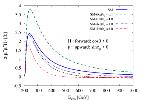
We see that all four anomalous couplings contribute to the partial cross-section, which can now be parametrized as
| (42) |
If only one anomalous coupling were to be non-zero, then the measurement of this partial cross-section would be sensitive to
| (43) |
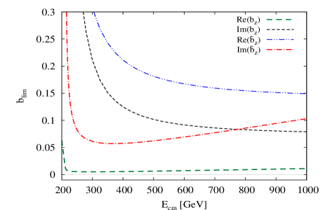
Here is the degree of statistical significance, is the integrated luminosity of the collider and is the fractional systematic error. In Fig. 10, we show a simple () limit on anomalous couplings, obtained using Fig. 9, for an integrated luminosity of 500 fb-1. A measurement of will thus be sensitive to values of lying above the corresponding curve.
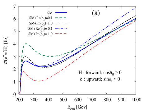
A similar exercise can be done for , and in Fig. 11(a) we display the partial cross-section for the same as a function of the center-of-mass energy. The presence of an additional -channel diagram changes the behaviour of the partial cross-section and hence that of the limits that could be inferred in a fashion analogous to Fig. 9.
For and , the bounds of Table 2 are much better than the limits shown in Fig. 10. This indicates that asymmetries with appropriate symmetry properties and combinations of various final states can be used efficiently to obtain stringent constraints on anomalous couplings.
For , on the other hand, the limit obtained using is only comparable to the one obtained using just the partial rate after accounting for degrees of significance. However, the limit from is subject to the assumption that all other anomalous couplings are zero, while the one obtained using is independent of any other anomalous coupling. Once again this underscores the importance of specific observables, such as , which receive a contribution from only one of the anomalous coupling, thus allowing us to obtain a robust constraint.
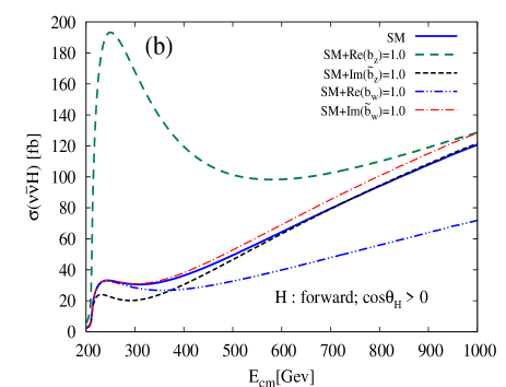
And finally, we look at the channel, where both and vertices contribute thus doubling the number of anomalous couplings involved. Since the final state fermions, the neutrinos, are not detectable, it is meaningless to construct the partial cross-section . Instead we add and to form the “forward” cross-section, i.e. the Higgs boson is constrained to be in the forward direction, and the dependence is displayed in Fig. 11(b). The size of the anomalous contribution in these figures gives an idea about the sensitivity to that particular coupling.
Appendix B Expressions for
In this appendix, we list the square of invariant matrix element for the various processes considered in the text. To begin with, we define the fermion- vertices by
In considering a process such as , it is further convenient to devise a notation for scalar products such as
| (44) |
and similarly for the multitude of propagators that one encounters, namely
| (45) | |||||
| (46) | |||||
| (47) |
we have, for where is any massless fermion,
| (48) |
For , the expressions are a bit more complicated, and
| (49) |
where,
| (50) |
| (51) |
And finally, for ,
| (52) |
where,
| (53) | |||||
| (54) | |||||
| (55) | |||||
In the propagators, we ignore the contribution proportional to except for , which goes on-shell, and cannot be ignored, in general.
References
- (1) For a review, see for example, R. M. Godbole, [arXiv:hep-ph/0205114], Volume 4, Jubilee Issue of the Indian Journal of Physics, pp. 44-83, 2004, Guest Editors: A. Raychaudhuri and P. Mitra.
-
(2)
ALEPH, DELPHI, L3 and OPAL Collaborations,
The LEP Working Group for Higgs Boson Searches,
Phys. Lett. B 565, 61 (2003);
see also http://lephiggs.web.cern.ch/LEPHIGGS/ -
(3)
LEP Electroweak Working Group,
http://lepewwg.web.cern.ch/LEPEWWG/ - (4) R. Akers et al. [OPAL Collaboration], Z. Phys. C 61, 19 (1994); D. Buskulic et al. [ALEPH Collaboration], Z. Phys. C 62, 539 (1994); M. Acciarri et al. [L3 Collaboration], Z. Phys. C 62, 551 (1994); P. Abreu et al. [DELPHI Collaboration], Z. Phys. C 67, 69 (1995); D. Antreasyan et al. [Crystal Ball Collaboration], Phys. Lett. B 251, 204 (1990); P. Franzini et al., Phys. Rev. D 35, 2883 (1987); J. Kalinowski and M. Krawczyk, Phys. Lett. B 361, 66 (1995) [arXiv:hep-ph/9506291]; D. Choudhury and M. Krawczyk, Phys. Rev. D 55, 2774 (1997) [arXiv:hep-ph/9607271].
- (5) M. Carena, J. R. Ellis, A. Pilaftsis and C. E. M. Wagner, Nucl. Phys. B586, 92 (2000); A. Mendez and A. Pomarol, Phys. Lett. B 279, 98 (1992); J. F. Gunion, H. E. Haber and J. Wudka, Phys. Rev. D 43, 904 (1991); J. F. Gunion, B. Grzadkowski, H. E. Haber and J. Kalinowski, Phys. Rev. Lett. 79, 982 (1997) [hep-ph/9704410]; I. F. Ginzburg, M. Krawczyk and P. Osland, hep-ph/0211371.
- (6) G. Abbiendi et al. [OPAL Collaboration], Eur. Phys. J. C 37, 49 (2004); ALEPH, DELPHI, L3 and OPAL Collaborations, The LEP Working Group for Higgs Boson Searches, LHWG-Note 2004-01.
- (7) See for example, J. R. Forshaw, Pramana 63, 1119 (2004) and discussion therein; see also D. Choudhury, T. M. P. Tait and C. E. M. Wagner, Phys. Rev. D 65, 053002 (2002) [arXiv:hep-ph/0109097].
- (8) ATLAS Collaboration, Detector and Physics Performance Technical Design Report, CERN-LHCC-99-14 & 15 (1999); CMS Collaboration, Technical Design Report, CERN-LHCC-97-10 (1997).
- (9) See for example, M. Drees, R. M. Godbole, P. Roy, Theory and Phenomenology of Sparticles , World Scientific, 2004.
- (10) For a brief review, see for example, R. M. Godbole, S. Kraml, M. Krawczyk, D. J. Miller, P. Niezurawski and A. F. Zarnecki, arXiv:hep-ph/0404024 and references therein.
- (11) R. L. Kelly and T. Shimada, Phys. Rev. D 23, 1940 (1981); P. Kalyniak, J. N. Ng, P. Zakarauskas, Phys. Rev. D 29, 502 (1984). W. Kilian, M. Kramer and P. M. Zerwas, Phys. Lett. B 373, 135 (1996) [arXiv:hep-ph/9512355].
- (12) J. C. Romao and A. Barroso, Phys. Lett. B 185, 195 (1987).
- (13) R. Rattazzi, Z. Phys. C 40, 605 (1988).
- (14) K. Hagiwara and M. L. Stong, Z. Phys. C 62, 99 (1994).
- (15) H. J. He, Y. P. Kuang, C. P. Yuan and B. Zhang, Phys. Lett. B 554, 64 (2003) [arXiv:hep-ph/0211229].
- (16) K. Hagiwara, S. Ishihara, R. Szalapski and D. Zeppenfeld, Phys. Rev. D 48, 2182 (1993); K. Hagiwara, R. Szalapski and D. Zeppenfeld, Phys. Lett. B 318, 155 (1993) [arXiv:hep-ph/9308347].
- (17) G. J. Gounaris, F. M. Renard and N. D. Vlachos, Nucl. Phys. B 459, 51 (1996) [arXiv:hep-ph/9509316].
- (18) B. Zhang, Y. P. Kuang, H. J. He and C. P. Yuan, Phys. Rev. D 67, 114024 (2003) [arXiv:hep-ph/0303048].
- (19) T. Plehn, D. Rainwater and D. Zeppenfeld, Phys. Rev. Lett. 88 051801 (2002)
- (20) K. Hagiwara, S. Ishihara, J. Kamoshita and B. A. Kniehl, Eur. Phys. J. C 14, 457 (2000) [arXiv:hep-ph/0002043].
- (21) D. Atwood and A. Soni, Phys. Rev. D 45, 2405 (1992).
- (22) T. Han and J. Jiang, Phys. Rev. D 63, 096007 (2001)
- (23) P. Niezurawski, A. F. Zarnecki and M. Krawczyk, Acta Phys. Polon. B 36, 833 (2005) [arXiv:hep-ph/0410291].
- (24) B. A. Kniehl, Nucl. Phys. B 352, 1 (1991); Nucl. Phys. B 357, 439 (1991)
- (25) M. C. Gonzalez-Garcia, Int. J. Mod. Phys. A 14, 3121 (1999) [arXiv:hep-ph/9902321]. V. Barger, T. Han, P. Langacker, B. McElrath and P. Zerwas, Phys. Rev. D 67, 115001 (2003) [arXiv:hep-ph/0301097].
- (26) A. Mendez and A. Pomarol, Phys. Lett. B 272, 313 (1991).
- (27) D. Choudhury, A. Datta and K. Huitu, Nucl. Phys. B 673, 385 (2003) [arXiv:hep-ph/0302141].
- (28) A. Pilaftsis and C. E. M. Wagner, Nucl. Phys. B 553, 3 (1999); M. Carena, H. E. Haber, H. E. Logan and S. Mrenna, Phys. Rev. D 65, 055005 (2002)
- (29) V. D. Barger, K.-m. Cheung, A. Djouadi, B. A. Kniehl and P. M. Zerwas, Phys. Rev. D 49, 79 (1994) [arXiv:hep-ph/9306270].
- (30) D. Choudhury, T. M. P. Tait and C. E. M. Wagner, Phys. Rev. D 65, 115007 (2002) [arXiv:hep-ph/0202162].
- (31) For a recent review, see A. Djouadi, arXiv:hep-ph/0503172.
- (32) M. Acciarri et al. [L3 Collaboration], Phys. Lett. B 439, 225 (1998); P. Abreu et al. [DELPHI Collaboration], Eur. Phys. J. C 9, 367 (1999); S. M. Xella-Hansen, M. Wing, D. J. Jackson, N. De Groot and C. J. S. Damerell, LC-PHSM-2003-061;
- (33) A. Denner, S. Dittmaier, M. Roth and M. M. Weber, Nucl. Phys. B 660, 289 (2003) [arXiv:hep-ph/0302198]; A. Denner, S. Dittmaier, M. Roth and M. M. Weber, Nucl. Phys. Proc. Suppl. 135, 88 (2004) [arXiv:hep-ph/0406335]; F. Boudjema et al., Phys. Lett. B 600, 65 (2004) [arXiv:hep-ph/0407065]; G. Belanger et al, Phys. Lett. B 559, 252 (2003) [arXiv:hep-ph/0212261]; Nucl. Phys. Proc. Suppl. 116, 353 (2003) [arXiv:hep-ph/0211268].
- (34) T. Hahn, S. Heinemeyer and G. Weiglein, Nucl. Phys. B 652, 229 (2003) [arXiv:hep-ph/0211204]; S. Heinemeyer and G. Weiglein, Nucl. Phys. Proc. Suppl. 89, 210 (2000); H. Eberl, W. Majerotto and V. C. Spanos, Nucl. Phys. B 657, 378 (2003) [arXiv:hep-ph/0210038].