General partonic structure for hadronic spin asymmetries

Abstract

The high energy and large $p_{T}$ inclusive polarized process, $(A,S_{A})+(B,S_{B})\to C+X$, is considered under the assumption of a generalized QCD factorization scheme. For the first time all transverse motions, of partons in hadrons and of hadrons in fragmenting partons, are explicitly taken into account; the elementary interactions are computed at leading order with noncollinear exact kinematics, which introduces many phases in the expressions of their helicity amplitudes. Several new spin and $\mbox{\boldmath$k$}_{\perp}$ dependent soft functions appear and contribute to the cross sections and to spin asymmetries; we put emphasis on their partonic interpretation, in terms of quark and gluon polarizations inside polarized hadrons. Connections with other notations and further information are given in some Appendices. The formal expressions for single and double spin asymmetries are derived. The transverse single spin asymmetry $A_{N}$, for $p^{\uparrow}\,p\to\pi\,X$ processes is considered in more detail, and all contributions are evaluated numerically by saturating unknown functions with their upper positivity bounds. It is shown that the integration of the phases arising from the noncollinear kinematics strongly suppresses most contributions to the single spin asymmetry, leaving at work predominantly the Sivers effect and, to a lesser extent, the Collins mechanism.

I Introduction and formalism

There is, at present, no completely rigorous theory of single spin asymmetries in hadron–hadron collisions and inclusive particle production. Rigorous results about how different physical processes, including hadronic ones, are related to each other via factorization, only exist for the restricted case of collinear kinematics. But it is precisely in this kinematic situation that one cannot generate single spin asymmetries at leading twist. Thus, the introduction of intrinsic $k_{\perp}$ is crucial for a model of single spin asymmetries and we are therefore forced to rely on an intuitively reasonable calculational approach, within QCD, assuming a simple factorization scheme. This effectively neglects the role of the soft factors related to the Wilson lines which occur in the rigorous definition of $k_{\perp}$ dependent parton densities and fragmentation functions.

In recent papers fu ; noi we have discussed such a formalism to compute cross sections for polarized and unpolarized inclusive processes, $A\,B\to C\,X$, fully taking into account parton intrinsic motion in distribution and fragmentation functions, as well as in the elementary dynamics. In particular, in Ref. noi the emphasis was on the importance of the many phases appearing in the computation of helicity amplitudes in noncollinear configurations, and their role in suppressing the contribution of the Collins mechanism col to transverse single spin asymmetries. Many other contributions to polarized and unpolarized cross sections, and to single and double spin asymmetries, were not discussed, referring to a later paper for the full treatment of the most complete case.

We consider here such a general case. Let us start from Eq. (8) of Ref. noi :

$$\frac{E_{C}\,d\sigma^{(A,S_{A})+(B,S_{B})\to C+X}}{d^{3}\mbox{\boldmath$p$}_{C}}=\!\!\!\!\!\sum_{a,b,c,d,\{\lambda\}} \!\!\!\int\frac{dx_{a}\,dx_{b}\,dz}{16\pi^{2}x_{a}x_{b}z^{2}s}\;d^{2}\mbox{\boldmath$k$}_{\perp a}\,d^{2}\mbox{\boldmath$k$}_{\perp b}\,d^{3}\mbox{\boldmath$k$}_{\perp C}\,\delta(\bm{k}_{\perp C}\cdot\hat{\bm{p}}_{c})\,J(\bm{k}_{\perp C})$$

$$\times \rho_{\lambda^{\,}_{a},\lambda^{\prime}_{a}}^{a/A,S_{A}}\,\hat{f}_{a/A,S_{A}}(x_{a},\mbox{\boldmath$k$}_{\perp a})\>\rho_{\lambda^{\,}_{b},\lambda^{\prime}_{b}}^{b/B,S_{B}}\,\hat{f}_{b/B,S_{B}}(x_{b},\mbox{\boldmath$k$}_{\perp b})$$

$$\times \hat{M}_{\lambda^{\,}_{c},\lambda^{\,}_{d};\lambda^{\,}_{a},\lambda^{\,}_{b}}\,\hat{M}^{*}_{\lambda^{\prime}_{c},\lambda^{\,}_{d};\lambda^{\prime}_{a},\lambda^{\prime}_{b}}\>\delta(\hat{s}+\hat{t}+\hat{u})\>\hat{D}^{\lambda^{\,}_{C},\lambda^{\,}_{C}}_{\lambda^{\,}_{c},\lambda^{\prime}_{c}}(z,\mbox{\boldmath$k$}_{\perp C})\>,$$

which gives the cross section for the polarized hadronic process $(A,S_{A})+(B,S_{B})\to C+X$ as a (factorized) convolution of all possible hard elementary QCD processes, $ab\to cd$, with soft partonic polarized distribution and fragmentation functions. In Eq. (I) $\hat{s},\hat{t}$ and $\hat{u}$ are the Mandelstam variables for the partonic reactions and the detailed connection between the hadronic and the partonic kinematical variables is given in full in Appendix A.

Let us clarify the physical meaning of Eq. (I) – our starting point – by making detailed comments on its notation and contents.

• $A$ and $B$ are initial spin 1/2 hadrons (typically, two protons), in pure spin states denoted by $S_{A}$ and $S_{B}$ respectively, with corresponding polarization vectors $\mbox{\boldmath$P$}^{A}$ and $\mbox{\boldmath$P$}^{B}$ (notice that $\mbox{\boldmath$P$}^{A,B}$ are actually pseudovectors). We set $S_{A,B}=0$ for unpolarized hadrons ($\mbox{\boldmath$P$}^{A,B}=$ 0). $E_{C}$ and $\mbox{\boldmath$p$}_{C}$ are the energy and three-momentum of the final detected particle (typically, a pion). Throughout the paper, we work in the $AB$ c.m. frame, assuming that hadron $A$ moves along the positive $Z_{cm}$-axis and hadron $C$ is produced in the $(XZ)_{cm}$ plane, with $(p_{C})_{X_{cm}}>0$. We define as transverse polarization for hadrons $A$ and $B$ the $Y_{cm}$-direction, often using the notation

  $$\uparrow\;{\rm for}\;P_{Y_{cm}}^{A}=1\;{\rm and}\;P_{Y_{cm}}^{B}=-1\quad\quad\quad\quad\downarrow\;{\rm for}\;P_{Y_{cm}}^{A}=-1\;{\rm and}\;P_{Y_{cm}}^{B}=1\>.$$ (2)

  The longitudinal spin states are labelled by their helicities: $\lambda_{A,B}=\pm 1/2$ (sometimes just written as $\pm$) corresponding to $P_{Z_{cm}}^{A}=\pm 1$ and to $P_{Z_{cm}}^{B}=\mp 1$ respectively. The opposite signs for hadrons $A$ and $B$ originate from the fact that their helicity frames, as reached from the overall c.m. frame, have opposite $Y$ and $Z$ axes elliot , see Eq. (199). The general case of hadrons transversely polarized along a generic direction $\phi_{S_{A}}$ in the $(XY)_{cm}$ plane is treated in Appendix B.

• The notation $\{\lambda\}$ implies a sum over all helicity indices. $x_{a}$, $x_{b}$ and $z$ are the usual light-cone momentum fractions, of partons in hadrons ($x_{a,b}$) and hadrons in partons ($z$). $\mbox{\boldmath$k$}_{\perp a}\,(\mbox{\boldmath$k$}_{\perp b})$ and $\mbox{\boldmath$k$}_{\perp C}$ are respectively the transverse momenta of parton $a\,(b)$ with respect to hadron $A\,(B)$, and of hadron $C$ with respect to parton $c$. We consider all partons as massless, neglecting heavy quark contributions.

• With massless partons, the function $J$ is given by fu

  $$J(\bm{k}_{\perp C})=\frac{\left(E_{C}+\sqrt{\bm{p}^{2}_{C}-\bm{k}^{2}_{\perp C}}\right)^{2}}{4(\bm{p}^{2}_{C}-\bm{k}^{2}_{\perp C})}\>\cdot$$ (3)

• $\rho_{\lambda^{\,}_{a},\lambda^{\prime}_{a}}^{a/A,S_{A}}$ is the helicity density matrix of parton $a$ inside the polarized hadron $A$, with spin state $S_{A}$. Similarly for parton $b$ inside hadron $B$ with spin $S_{B}$. Notice that the helicity density matrix describes the spin orientation of a particle in its helicity frame elliot ; for a spin 1/2 particle, Tr$\,(\sigma_{i}\rho)=P_{i}$ is the $i$-component of the polarization vector $P$ in the helicity rest frame of the particle. Obviously, for a massless parton there is no rest frame and the helicity frame is defined as the standard frame elliot in which its four-momentum is $p^{\mu}=(p,0,0,p)$ (see also Appendix D). $\hat{f}_{a/A,S_{A}}(x_{a},\mbox{\boldmath$k$}_{\perp a})$ is the distribution function of the unpolarized parton $a$ inside the polarized hadron $A$. We shall also denote by $\hat{f}^{a}_{s_{i}/S_{J}}$ the number densities of partons $a$, with spin along the $i$-axis, inside a hadron $A$ with spin along the $J$-axis: $i=x,y,z$ stand for directions in the parton helicity frame, whereas $J=X,Y,Z$ refer to the hadron helicity rest frame.

• The $\hat{M}_{\lambda^{\,}_{c},\lambda^{\,}_{d};\lambda^{\,}_{a},\lambda^{\,}_{b}}$’s are the helicity amplitudes for the elementary process $ab\to cd$, normalized so that the unpolarized cross section, for a collinear collision, is given by

  $$\frac{d\hat{\sigma}^{ab\to cd}}{d\hat{t}}=\frac{1}{16\pi\hat{s}^{2}}\frac{1}{4}\sum_{\lambda^{\,}_{a},\lambda^{\,}_{b},\lambda^{\,}_{c},\lambda^{\,}_{d}}|\hat{M}_{\lambda^{\,}_{c},\lambda^{\,}_{d};\lambda^{\,}_{a},\lambda^{\,}_{b}}|^{2}\,.$$ (4)

• $\hat{D}^{\lambda^{\,}_{C},\lambda^{\prime}_{C}}_{\lambda^{\,}_{c},\lambda^{\prime}_{c}}(z,\mbox{\boldmath$k$}_{\perp C})$ is the product of fragmentation amplitudes for the $c\to C+X$ process

  $$\hat{D}^{\lambda^{\,}_{C},\lambda^{\prime}_{C}}_{\lambda^{\,}_{c},\lambda^{\prime}_{c}}=\>\mathrel{\mathop{\kern 0.0pt\hbox to0.0pt{\hbox{$\sum$}\hss}}\hbox{\kern-1.25pt$\displaystyle\int$}}_{X,\lambda_{X}}{\hat{\cal D}}_{\lambda^{\,}_{C},\,\lambda_{X};\lambda^{\,}_{c}}\,{\hat{\cal D}}^{*}_{\lambda^{\prime}_{C},\,\lambda_{X};\lambda^{\prime}_{c}}\,,$$ (5)

  where the $\mathrel{\mathop{\kern 0.0pt\hbox to0.0pt{\hbox{$\sum$}\hss}}\hbox{\kern-1.25pt$\displaystyle\int$}}_{X,\lambda_{X}}$ stands for a spin sum and phase space integration over all undetected particles, considered as a system $X$. The usual unpolarized fragmentation function $D_{C/c}(z)$, i.e. the number density of hadrons $C$ resulting from the fragmentation of an unpolarized parton $c$ and carrying a light-cone momentum fraction $z$, is given by

  $$D_{C/c}(z)=\frac{1}{2}\sum_{\lambda^{\,}_{c},\lambda^{\,}_{C}}\int d^{2}\mbox{\boldmath$k$}_{\perp C}\,\hat{D}^{\lambda^{\,}_{C},\lambda^{\,}_{C}}_{\lambda^{\,}_{c},\lambda^{\,}_{c}}(z,\mbox{\boldmath$k$}_{\perp C})\,.$$ (6)

Eq. (I) is written in a factorized form, separating the soft, long distance from the hard, short distance contributions. The hard part is computable in perturbative QCD (pQCD), while information on the soft one has to be extracted from other experiments or modeled. As already mentioned and discussed in Ref. noi , such a factorization with noncollinear kinematics has never been formally proven. Indeed, studies of factorization piet ; metz ; ji , comparing semi-inclusive deep inelastic scattering (SIDIS) and Drell-Yan reactions have indicated unexpected modifications of simple factorization, and the situation for inclusive particle production in hadron–hadron collisions is not yet resolved. Thus, our approach can only be considered as a reasonable phenomenological model. Of course, the perturbative calculation of the hard part is only reliable if the hard scale – in this case the square of the transverse momentum of the final hadron, $p_{T}^{2}$ – is large enough; in our case $p_{T}^{2}\geq 2.25$ (GeV/$c$)². It turns out that the data demand fu an average value of $k_{\perp}^{2}\simeq 0.64$ (GeV/$c$)² for the intrinsic transverse momentum of the parton distributions. This is relatively small compared to 2.25 (GeV/$c$)², but complications can arise from the tail of the Gaussian distribution, as was discussed in Ref. fu and will be commented on in Section V.

The intrinsic motion arises both from parton confinement and from QCD gluon emission. In that, our approach, based on perturbative computations performed at LO in the strong coupling constant, with noncollinear kinematics, could partially and effectively contain some of the effects related to soft gluon emissions and the threshold resummation of large logarithmic perturbative corrections, recently performed within proper collinear factorization dfv . A study of weighted single spin asymmetries for double-inclusive production in hadron-hadron collisions, based on $\mbox{\boldmath$k$}_{\perp}$ factorization using a diagrammatic approach, has appeared very recently piet .

In the next Section we discuss in detail the soft contributions to Eq. (I), related to parton distribution and fragmentation functions, while in Section III we give the explicit analytical expressions of all elementary amplitudes, convoluted with the corresponding soft functions. Some contributions to the unpolarized cross section and the transverse Single Spin Asymmetry (SSA) are analytically discussed in Section IV. Numerical estimates of the maximal contributions of the different spin mechanisms, both to the cross section and the transverse SSA, are presented and discussed in Section V. General conclusions and comments are given in Section VI. Finally, the full noncollinear partonic kinematics and its relation with the overall hadronic variables is discussed, for convenience and completeness, in Appendix A; the formal relationships between the hadron and the parton polarization are widely studied in Appendix B, and the connection with other formalims is explicitely worked out in Appendix C. Useful definitions of helicity frames are given in Appendix D.

II Soft physics

Although Eq. (I) has already a clear physical interpretation, we would like to express the parton density matrix elements in terms of parton polarizations, so that, when performing the helicity sums, each term has a direct partonic meaning.

Notice that the parton polarizations are, of course, related to their parent hadron polarizations. The way the hadron spin is transferred to the partons can be formally described, in general, by bilinear combinations of the helicity amplitudes for the process $A\to a+X$ (distribution amplitudes) noi ; noi95 . Therefore, one could equally well interpret Eq. (I) either in terms of parton polarizations or in terms of the distribution amplitudes. We follow here the former approach, which is somewhat more direct. However, the latter approach offers a deeper understanding of some of the basic properties of our factorized scheme (e.g. the parity properties) and allows a direct comparison with other formalims used to describe the same spin effects. In Appendix B we give the full correspondence between parton polarizations and the distribution amplitudes, and in Appendix C we derive the explicit relations between our formalism and that of the Amsterdam group amst .

II.1 Quark polarizations

The helicity density matrix of quark $a$ can be written in terms of the quark polarization vector components, $\mbox{\boldmath$P$}^{a}=(P^{a}_{x},P^{a}_{y},P^{a}_{z})=(P_{T}^{a}\cos\phi_{s_{a}},P_{T}^{a}\sin\phi_{s_{a}},P_{L}^{a})$, as

$$\rho_{\lambda^{\,}_{a},\lambda^{\prime}_{a}}^{a/A,S_{A}}={\left(\begin{array}[]{cc}\rho_{++}^{a}&\rho_{+-}^{a}\\ \rho_{-+}^{a}&\rho_{--}^{a}\end{array}\right)}_{\!\!\!\!A,S_{A}}\!\!\!\!\!\!\!=\frac{1}{2}\,{\left(\begin{array}[]{cc}1+P^{a}_{z}&P^{a}_{x}-iP^{a}_{y}\\ P^{a}_{x}+iP^{a}_{y}&1-P^{a}_{z}\end{array}\right)}_{\!\!\!\!A,S_{A}}\!\!\!\!\!\!\!=\frac{1}{2}\,{\left(\begin{array}[]{cc}1+P^{a}_{L}&P^{a}_{T}\,e^{-i\phi_{s_{a}}}\\ P^{a}_{T}\,e^{i\phi_{s_{a}}}&1-P^{a}_{L}\end{array}\right)}_{\!\!\!\!A,S_{A}}\!\!\!,$$ (7)

where, as explained above, the $x,y$ and $z$-directions are those of the helicity frame of parton $a$. Eq. (7) satisfies the well known general properties:

$$\rho^{a}_{++}+\rho^{a}_{--}=1$$ (8)

$$\rho^{a}_{++}-\rho^{a}_{--}=P^{a}_{z}=P_{L}^{a}$$ (9)

$$2\,{\rm Re}\rho^{a}_{-+}=2\,{\rm Re}\rho^{a}_{+-}=P^{a}_{x}=P_{T}^{a}\,\cos\phi_{s_{a}}$$ (10)

$$2\,{\rm Im}\rho^{a}_{-+}=-2\,{\rm Im}\rho^{a}_{+-}=P^{a}_{y}=P_{T}^{a}\,\sin\phi_{s_{a}}\,.$$ (11)

When performing the sum over the helicity indices $\lambda^{\,}_{a},\lambda^{\prime}_{a}$ and $\lambda^{\,}_{b},\lambda^{\prime}_{b}$ in Eq. (I), one obtains products of terms of the form

$$(P^{a}_{j}\,\hat{f}_{a/A,S_{A}})=\hat{f}^{a}_{s_{j}/S_{A}}-\hat{f}^{a}_{-s_{j}/S_{A}}\equiv\Delta\hat{f}^{a}_{s_{j}/S_{A}}\>,$$ (12)

where $j=x,y,z$. Similarly for parton $b$ inside hadron $B$. We use the notations:

$$(P^{a}_{j}\,\hat{f}_{a/A,S_{Y}})=\Delta\hat{f}_{s_{j}/S_{Y}}^{a}=\hat{f}_{s_{j}/\uparrow}^{a}-\hat{f}_{-s_{j}/\uparrow}^{a}\equiv\Delta\hat{f}_{s_{j}/\uparrow}^{a}(x_{a},\mbox{\boldmath$k$}_{\perp a})$$ (13)

$$(P^{a}_{j}\,\hat{f}_{a/A,S_{Z}})=\Delta\hat{f}_{s_{j}/S_{Z}}^{a}=\hat{f}_{s_{j}/+}^{a}-\hat{f}_{-s_{j}/+}^{a}\equiv\Delta\hat{f}_{s_{j}/+}^{a}(x_{a},\mbox{\boldmath$k$}_{\perp a})$$ (14)

$$(\hat{f}_{a/A,S_{Y}})=\hat{f}_{a/A}(x_{a},k_{\perp a})+\frac{1}{2}\,\Delta\hat{f}_{a/S_{Y}}(x_{a},\mbox{\boldmath$k$}_{\perp a})\,.$$ (15)

These amount to eight independent quantities, which represent the ($\mbox{\boldmath$k$}_{\perp}$ unintegrated) distribution functions of partons $a\,(=q,\bar{q})$ with polarization $\mbox{\boldmath$P$}^{a}$ (defined in the partonic helicity frame) inside hadron $A$ with spin $S_{A}$ (specified in the hadronic helicity frame). All of these functions have a simple direct physical meaning: for instance, the $x$-component of Eq. (13) – $(P^{a}_{x}\,\hat{f}_{a/A,S_{Y}})$ – represents the amount of polarization along the $x$-axis (in the partonic helicity frame) carried by partons $a$ inside a transversely polarized hadron $(A,S_{Y})$; $(P^{a}_{y}\,\hat{f}_{a/A,S_{Y}})$ is related to the $\mbox{\boldmath$k$}_{\perp}$ dependent transversity distribution, which, upon integration over $d^{2}\mbox{\boldmath$k$}_{\perp}$, gives the familiar transversity function $h^{q}_{1}(x)$ or $\Delta_{T}q(x)$ (see also Appendix B). Similarly, the $z$-component of Eq. (14) – $(P^{a}_{z}\,\hat{f}_{a/A,S_{Z}})$ – is the unintegrated helicity distribution, which, once integrated over the transverse momentum, gives the usual helicity distribution $\Delta q(x)$ or $g^{q}_{1}(x)$.

Notice that two independent distribution functions appear in the definition of $\hat{f}_{a/A,S_{Y}}$, which is the only term in the sum over $\lambda^{\,}_{a},\lambda^{\prime}_{a}$ which corresponds to parton $a$ being unpolarized: $\hat{f}_{a/A}(x_{a},k_{\perp a})$, the unintegrated number density of unpolarized partons $a$ inside the unpolarized proton $A$, and $\Delta\hat{f}_{a/S_{Y}}$, the Sivers function siv . The latter permits the number density of unpolarized partons $a$ to depend upon the transverse polarization of the parent hadron $A$. In general, for a hadron $A$ in a pure spin state $S_{A}$ and corresponding unit polarization vector $\hat{\mbox{\boldmath$P$}}^{A}$, one has:

$$\Delta\hat{f}_{a/S_{A}}\,(x_{a},\mbox{\boldmath$k$}_{\perp a}) \equiv \hat{f}_{a/S_{A}}\,(x_{a},\mbox{\boldmath$k$}_{\perp a})-\hat{f}_{a/-S_{A}}\,(x_{a},\mbox{\boldmath$k$}_{\perp a})$$ (16)

$$= \Delta^{N}\hat{f}_{a/A^{\uparrow}}\,(x_{a},k_{\perp a})\>(\hat{\mbox{\boldmath$p$}}_{A}\times\hat{\mbox{\boldmath$k$}}_{\perp a})\cdot\hat{\mbox{\boldmath$P$}}^{A}\>.$$

In the last term of the above expression we have explicitly extracted the angular dependences, according to the so-called “Trento conventions” trento : $\hat{\mbox{\boldmath$p$}}_{A}$ is the unit vector along the hadron $A$ three-momentum, $k_{\perp a}=|\mbox{\boldmath$k$}_{\perp a}|$ and $\hat{\mbox{\boldmath$k$}}_{\perp a}=\mbox{\boldmath$k$}_{\perp a}/k_{\perp a}$. Parity invariance allows to have a non-zero Sivers function only for transverse spin, $\hat{\mbox{\boldmath$p$}}_{A}\cdot\hat{\mbox{\boldmath$P$}}^{A}=0$. Often $\Delta^{N}\hat{f}_{a/A^{\uparrow}}\,(x_{a},k_{\perp a})$ alone is referred to as the Sivers function (see Appendix B for related expressions). For a generic transverse polarization direction $\hat{\mbox{\boldmath$P$}}^{A}=(\cos\phi_{S_{A}},\,\sin\phi_{S_{A}},\,0)$, one has $\Delta\hat{f}_{a/S_{A}}\,(x_{a},\mbox{\boldmath$k$}_{\perp a})=\Delta^{N}\hat{f}_{a/A^{\uparrow}}\,(x_{a},k_{\perp a})\,\sin(\phi_{S_{A}}-\phi_{a})$, where $\phi_{a}$ is the azimuthal angle (in the hadronic c.m. frame) of $\mbox{\boldmath$k$}_{\perp a}$.

According to our configuration the hadron transverse polarization is chosen along the $+Y$-direction ($\uparrow$); notice that $Y=Y_{cm}$ for the hadron moving along the $+Z_{cm}$-direction, while $Y=-Y_{cm}$ for the hadron moving along $-Z_{cm}$, as already noticed after Eq. (2). Then, Eq. (16) reads:

$$\Delta\hat{f}_{a/S_{Y}}\,(x_{a},\mbox{\boldmath$k$}_{\perp a}) \equiv \hat{f}_{a/S_{Y}}\,(x_{a},\mbox{\boldmath$k$}_{\perp a})-\hat{f}_{a/-S_{Y}}\,(x_{a},\mbox{\boldmath$k$}_{\perp a})$$ (17)

$$= \Delta^{N}\hat{f}_{a/A^{\uparrow}}\,(x_{a},k_{\perp a})\>\cos\phi_{a}\>.$$

Similarly, the Boer-Mulders mechanism amst ; dan (see Appendix B) allows partons to be transversely polarized inside an unpolarized parent hadron. In general, this can be expressed by:

$$P^{a}_{j}\,\hat{f}_{a/A} = \hat{f}_{s_{j}/A}^{a}(x_{a},\mbox{\boldmath$k$}_{\perp a})-\hat{f}_{-s_{j}/A}^{a}(x_{a},\mbox{\boldmath$k$}_{\perp a})\equiv\Delta\hat{f}_{s_{j}/A}^{a}(x_{a},\mbox{\boldmath$k$}_{\perp a})$$ (18)

$$= \Delta^{N}\hat{f}_{a^{\uparrow}/A}\,(x_{a},k_{\perp a})\>(\hat{\mbox{\boldmath$p$}}_{A}\times\hat{\mbox{\boldmath$k$}}_{\perp a})_{j}\>,$$

where $P^{a}_{j}$ is the $j$-component of the parton polarization in the parton helicity frame ($j=x,y,z$). The above equation can also be written as trento

$$\Delta\hat{f}_{s/A}^{a}(x_{a},\mbox{\boldmath$k$}_{\perp a}) \equiv \hat{f}_{s/A}^{a}(x_{a},\mbox{\boldmath$k$}_{\perp a})-\hat{f}_{-s/A}^{a}(x_{a},\mbox{\boldmath$k$}_{\perp a})$$

$$= \Delta^{N}\hat{f}_{a^{\uparrow}/A}\,(x_{a},k_{\perp a})\>(\hat{\mbox{\boldmath$p$}}_{A}\times\hat{\mbox{\boldmath$k$}}_{\perp a})\cdot\hat{\mbox{\boldmath$P$}}^{a}\>,$$ (19)

where $s$ and $\hat{\mbox{\boldmath$P$}}^{a}$ denote respectively a generic parton spin state and the corresponding unit polarization vector, in the parton helicity frame (as reached from the parent hadron helicity frame). Notice that, according to our configuration, in the hadronic c.m. frame $\hat{\mbox{\boldmath$y$}}$ points along the $\hat{\mbox{\boldmath$Z$}}_{cm}\times\hat{\mbox{\boldmath$k$}}_{\perp a}$ direction, Eq. (200). It follows that for nucleons moving respectively along the $\pm Z_{cm}$-direction one has

$$\Delta\hat{f}_{s_{y}/A}^{a}(x_{a},\mbox{\boldmath$k$}_{\perp a})=\pm\Delta^{N}\hat{f}_{a^{\uparrow}/A}\,(x_{a},k_{\perp a})\>.$$ (20)

It also follows that the analogous function for the $x$-direction is zero, $\Delta\hat{f}_{s_{x}/A}^{a}=0$. The function $\Delta^{N}\hat{f}_{a^{\uparrow}/A}\,(x_{a},k_{\perp a})$ alone is often referred to as the Boer-Mulders function.

Moreover, one can show that the Boer-Mulders function is the same which appears in the $y$-component of Eq. (14),

$$\Delta\hat{f}_{s_{y}/A}^{a}=(P^{a}_{y}\,\hat{f}_{a/A})=(P^{a}_{y}\,\hat{f}_{a/A,S_{Z}})=\Delta\hat{f}_{{s_{y}}/+}^{a}\>,$$ (21)

due to parity invariance.

It is worth mentioning that the function $(P^{a}_{y}\,\hat{f}_{a/S_{Y}})=\Delta\hat{f}^{a}_{s_{y}/S_{Y}}\equiv\Delta\hat{f}^{a}_{s_{y}/\uparrow}$ can be decomposed into two terms, the Boer-Mulders term which is independent of the hadron transverse polarization, and a term which changes sign when the hadron polarization direction is reversed:

$$\Delta\hat{f}^{a}_{s_{y}/S_{Y}}=\Delta\hat{f}^{a}_{s_{y}/A}+\Delta^{-}\hat{f}^{a}_{s_{y}/S_{Y}}\,,$$ (22)

with

$$\Delta^{-}\hat{f}^{a}_{s_{y}/S_{Y}}\equiv\frac{1}{2}\,\left[\Delta\hat{f}^{a}_{s_{y}/\uparrow}-\Delta\hat{f}^{a}_{s_{y}/\downarrow}\right]=-\Delta^{-}\hat{f}^{a}_{s_{y}/-S_{Y}}\,.$$ (23)

Notice that

$$\Delta\hat{f}^{a}_{s_{x}/S_{Y}}=\Delta^{-}\hat{f}^{a}_{s_{x}/S_{Y}}=-\Delta\hat{f}^{a}_{s_{x}/-S_{Y}}\,.$$

II.2 Gluon polarizations

Let us now consider the gluon sector (a first study of the unintegrated gluon distribution functions can be found in Ref. mr01 ). The helicity density matrix for a massless particle with spin $1$ can be written as

$$\rho_{\lambda_{g}^{\,},\lambda^{\prime}_{g}}^{g/A,S_{A}}=\frac{1}{2}\,{\left(\begin{array}[]{cc}1+P_{z}^{g}&\mathcal{T}_{1}^{g}-i\mathcal{T}_{2}^{g}\\ \mathcal{T}_{1}^{g}+i\mathcal{T}_{2}^{g}&1-P_{z}^{g}\end{array}\right)}_{\!\!\!\!A,S_{A}}\!\!\!\!\!\!\!=\frac{1}{2}\,{\left(\begin{array}[]{cc}1+P^{g}_{circ}&-P^{g}_{lin}\,e^{-2i\phi}\\ -P^{g}_{lin}\,e^{2i\phi}&1-P^{g}_{circ}\end{array}\right)}_{\!\!\!\!A,S_{A}}\!\!\!,$$ (24)

and we consider it for a gluon $g$ inside the hadron A, in a spin state $S_{A}$. Eq. (24) refers, in general, to a mixture of circularly and linearly polarized states. $P_{circ}^{g}$ corresponds to $P_{z}^{g}$, the gluon longitudinal polarization. The off-diagonal elements of Eq. (24) are related to the linear polarization of the gluons in the $(xy)$ plane at an angle $\phi$ to the $x$-axis. The $x$, $y$ and $z$ axes refer to the standard gluon helicity frame, in which its momentum is $p^{\mu}=(p,0,0,p)$. $P_{lin}^{g}$ is expressed in terms of the parameters $\mathcal{T}_{1}^{g}$ and $\mathcal{T}_{2}^{g}$, which are closely related to the Stokes parameters used in classical optics; they play a role formally analogous to that of the $x$ and $y$-components of the quark polarization vector in the quark sector. The use of the parameters $\mathcal{T}_{1}^{g}$ and $\mathcal{T}_{2}^{g}$ makes the gluon distribution functions formally similar to those for the quarks and considerably simplifies all the formulae for the spin asymmetries given in Sections III and IV.

In analogy to the quark helicity density matrix, Eq. (24) shows that:

$$\rho^{g}_{++}+\rho^{g}_{--}=1$$ (25)

$$\rho^{g}_{++}-\rho^{g}_{--}=P^{g}_{z}=P^{g}_{circ}$$ (26)

$$2\,{\rm Re}\rho^{g}_{-+}=2\,{\rm Re}\rho^{g}_{+-}=\mathcal{T}_{1}^{g}=-P^{g}_{lin}\cos(2\phi)$$ (27)

$$2\,{\rm Im}\rho^{g}_{-+}=-2\,{\rm Im}\rho^{g}_{+-}=\mathcal{T}_{2}^{g}=-P^{g}_{lin}\sin(2\phi)\,.$$ (28)

As for the quark sector, there are eight independent gluon distribution functions, which, following Eqs. (13-15), we label as

$$(\mathcal{T}_{1}^{g}\,\hat{f}_{g/A,S_{Y}})\equiv\Delta\hat{f}_{{\mathcal{T}_{1}}/\uparrow}^{g}(x_{g},\mbox{\boldmath$k$}_{\perp g})$$ (29)

$$(\mathcal{T}_{2}^{g}\,\hat{f}_{g/A,S_{Y}})\equiv\Delta\hat{f}_{{\mathcal{T}_{2}}/\uparrow}^{g}(x_{g},\mbox{\boldmath$k$}_{\perp g})$$ (30)

$$(P^{g}_{z}\,\hat{f}_{g/A,S_{Y}})=\Delta\hat{f}_{s_{z}/S_{Y}}^{g}=\hat{f}_{s_{z}/\uparrow}^{g}-\hat{f}_{-s_{z}/\uparrow}^{g}\equiv\Delta\hat{f}_{s_{z}/\uparrow}^{g}(x_{g},\mbox{\boldmath$k$}_{\perp g})$$ (31)

$$(\mathcal{T}_{1}^{g}\,\hat{f}_{g/A,S_{Z}})\equiv\Delta\hat{f}_{{\mathcal{T}_{1}}/+}^{g}(x_{g},\mbox{\boldmath$k$}_{\perp g})$$ (32)

$$(\mathcal{T}_{2}^{g}\,\hat{f}_{g/A,S_{Z}})\equiv\Delta\hat{f}_{{\mathcal{T}_{2}}/+}^{g}(x_{g},\mbox{\boldmath$k$}_{\perp g})$$ (33)

$$(P^{g}_{z}\,\hat{f}_{g/A,S_{Z}})=\Delta\hat{f}_{s_{z}/S_{Z}}^{g}=\hat{f}_{s_{z}/+}^{g}-\hat{f}_{-s_{z}/+}^{g}\equiv\Delta\hat{f}_{s_{z}/+}^{g}(x_{g},\mbox{\boldmath$k$}_{\perp g})$$ (34)

$$(\hat{f}_{g/A,S_{Y}})=\hat{f}_{g/A}(x_{g},\mbox{\boldmath$k$}_{\perp g})+\frac{1}{2}\,\Delta\hat{f}_{g/S_{Y}}(x_{g},\mbox{\boldmath$k$}_{\perp g})\,.$$ (35)

Notice that $\Delta\hat{f}_{s_{z}/+}^{g}(x_{g},\mbox{\boldmath$k$}_{\perp g})$ is the usual $\mbox{\boldmath$k$}_{\perp g}$ dependent gluon helicity distribution function $\Delta g(x_{g},\mbox{\boldmath$k$}_{\perp g})$. The interpretation of $\Delta\hat{f}_{{\mathcal{T}_{1},\mathcal{T}_{2}}/S_{A}}$ as difference of linearly polarized gluon distributions is discussed in the sequel and in Appendix B.

In analogy to Eqs. (22) and (23) we also define a new quantity which changes sign when the hadron polarization direction is reversed [see Eq. (157)]:

$$\Delta\hat{f}^{g}_{\mathcal{T}_{1}/\uparrow}=\Delta\hat{f}^{g}_{\mathcal{T}_{1}/A}+\Delta^{-}\hat{f}^{g}_{\mathcal{T}_{1}/\uparrow}\,,$$ (36)

with

$$\Delta^{-}\hat{f}^{g}_{\mathcal{T}_{1}/\uparrow}=\frac{1}{2}\,\left[\Delta\hat{f}^{g}_{\mathcal{T}_{1}/\uparrow}-\Delta\hat{f}^{g}_{\mathcal{T}_{1}/\downarrow}\right]=-\Delta^{-}\hat{f}^{g}_{\mathcal{T}_{1}/\downarrow}\,.$$ (37)

Although gluons cannot carry any transverse spin, there is a strong analogy between transversely polarized quarks and linearly polarized gluons; for example, analogous to the Boer–Mulders case for quarks, it is possible to have a linearly polarized gluon inside an unpolarized nucleon, corresponding to a non-vanishing $\mathcal{T}_{1}^{g}\hat{f}_{g/A}=\Delta\hat{f}_{\mathcal{T}_{1}/A}^{g}$. This mechanism has never been explored before. Its structure is linked to the spin 1 Cartesian tensor $T_{ij}$ (see, e.g., Section 3.1.12 of Ref. elliot ), which is symmetric and traceless. For a massless particle one has:

$$\quad\quad\quad\quad\quad\quad\quad\quad\quad T_{zz}=\frac{1}{\sqrt{6}}$$ (38)

$$\mathcal{T}_{1}=\sqrt{\frac{2}{3}}\left(T_{xx}-T_{yy}\right)\quad\quad\quad\quad\mathcal{T}_{2}=2\,\sqrt{\frac{2}{3}}\,T_{xy}\>.$$ (39)

Because of (38), the traceless condition and parity invariance, it is only possible to construct one scalar structure that depends non-trivially on the $T_{ij}$.

Using the three-vectors at our disposal – the gluon momentum $p$, its transverse momentum $\mbox{\boldmath$k$}_{\perp}$ and the parent hadron momentum $\mbox{\boldmath$p$}_{A}$ – we define:

$$\hat{\mbox{\boldmath$u$}}=\frac{\hat{\mbox{\boldmath$k$}}_{\perp}-(\hat{\mbox{\boldmath$k$}}_{\perp}\cdot\hat{\mbox{\boldmath$p$}})\,\hat{\mbox{\boldmath$p$}}}{\hat{\mbox{\boldmath$p$}}\cdot\hat{\mbox{\boldmath$p$}}_{A}}\quad\quad\quad\quad\quad\hat{\mbox{\boldmath$v$}}=\hat{\mbox{\boldmath$p$}}_{A}\times\hat{\mbox{\boldmath$k$}}_{\perp}$$ (40)

and introduce a tensor T whose components are $T_{ij}$. The only possible structure is then:

$$T_{ij}\,\hat{f}_{g/A}(x,k_{\perp}) = \sqrt{\frac{3}{2}}\,\left[\frac{1}{2}\,\Delta^{N}\hat{f}^{g}_{\mathcal{T}_{1}/A}(x,k_{\perp})\left(\hat{u}_{i}\hat{u}_{j}-\hat{v}_{i}\hat{v}_{j}\right)\right.$$ (41)

$$- \left.\frac{1}{6}\,\hat{f}_{g/A}(x,k_{\perp})\,\left(\hat{u}_{i}\hat{u}_{j}+\hat{v}_{i}\hat{v}_{j}-2\,\hat{p}_{i}\hat{p}_{j}\right)\right]\>,$$

which is the gluon tensorial analogue of Eq. (18). When nucleon $A$ moves along or opposite the $Z_{cm}$-axis this reduces to:

$$\mathcal{T}_{1}^{g}\hat{f}_{g/A}(x,\mbox{\boldmath$k$}_{\perp})=\Delta\hat{f}^{g}_{\mathcal{T}_{1}/A}(x,\mbox{\boldmath$k$}_{\perp})=\Delta^{N}\hat{f}^{g}_{\mathcal{T}_{1}/A}(x,k_{\perp})$$ (42)

in analogy to Eq. (20). Notice that, in this case, there is no $\pm$ sign on the r.h.s. of Eq. (42).

One can also show that the linear polarization $\mathcal{T}_{1}^{g}$ is independent of any longitudinal polarization of the nucleon, i.e.:

$$\Delta\hat{f}^{g}_{\mathcal{T}_{1}/A}=\Delta\hat{f}^{g}_{\mathcal{T}_{1}/A,S_{Z}}=\Delta\hat{f}^{g}_{\mathcal{T}_{1}/+}\>,$$ (43)

as in Eq. (21).

II.3 Quark and gluon fragmentation functions into unpolarized hadrons

As already mentioned in Section I, for the fragmentation process in general we define

$$\hat{D}^{\lambda^{\,}_{C},\lambda^{\prime}_{C}}_{\lambda^{\,}_{c},\lambda^{\prime}_{c}}(z,\mbox{\boldmath$k$}_{\perp C})=\>\mathrel{\mathop{\kern 0.0pt\hbox to0.0pt{\hbox{$\sum$}\hss}}\hbox{\kern-1.25pt$\displaystyle\int$}}_{X,\lambda_{X}}{\hat{\cal D}}_{\lambda^{\,}_{C},\lambda^{\,}_{X};\lambda^{\,}_{c}}(z,\mbox{\boldmath$k$}_{\perp C})\,{\hat{\cal D}}^{*}_{\lambda^{\prime}_{C},\lambda^{\,}_{X};\lambda^{\prime}_{c}}(z,\mbox{\boldmath$k$}_{\perp C})\,.$$ (44)

The analogous quantity for parton distributions can be found in Eq. (120). $\hat{{\cal D}}_{\lambda^{\,}_{C},\lambda^{\,}_{X};\lambda^{\,}_{c}}$ is the fragmentation amplitude describing the process $c\to C+X$ in which the parton $c$ from the elementary scattering $ab\to cd$ generates the detected final hadron $C$, with light-cone momentum fraction $z$ and transverse momentum $\mbox{\boldmath$k$}_{\perp C}$. If we denote by $\phi_{C}^{H}$ the azimuthal angle of the hadron $C$ in the parton $c$ helicity frame, we have

$$\hat{\cal D}_{\lambda^{\,}_{C},\lambda^{\,}_{X};\lambda^{\,}_{c}}(z,\mbox{\boldmath$k$}_{\perp C})={\cal D}_{\lambda^{\,}_{C},\lambda^{\,}_{X};\lambda^{\,}_{c}}(z,k_{\perp C})\>e^{i\lambda^{\,}_{c}\phi_{C}^{H}}\>,$$ (45)

similarly to Eq. (122) for parton distribution amplitudes. Eqs. (44) and (45) then give the generalized fragmentation function

$${\hat{D}}_{\lambda^{\,}_{c},\lambda^{\prime}_{c}}^{\lambda^{\,}_{C},\lambda^{\prime}_{C}}(z,\mbox{\boldmath$k$}_{\perp C})={D}_{\lambda^{\,}_{c},\lambda^{\prime}_{c}}^{\lambda^{\,}_{C},\lambda^{\prime}_{C}}(z,k_{\perp C})\>e^{i(\lambda^{\,}_{c}-\lambda^{\prime}_{c})\phi_{C}^{H}}\>,$$ (46)

while the corresponding generalized distribution function is given in Eq. (123).

If hadron $C$ is unpolarized, the generalized fragmentation function ${\hat{D}}$ simply becomes

$${\hat{D}}_{\lambda^{\,}_{c},\lambda^{\prime}_{c}}^{C/c}(z,\mbox{\boldmath$k$}_{\perp C})=\sum_{\lambda^{\,}_{C}}\hat{D}^{\lambda^{\,}_{C},\lambda^{\,}_{C}}_{\lambda^{\,}_{c},\lambda^{\prime}_{c}}(z,\mbox{\boldmath$k$}_{\perp C})={D}_{\lambda^{\,}_{c},\lambda^{\prime}_{c}}^{C/c}(z,k_{\perp C})\>e^{i(\lambda^{\,}_{c}-\lambda^{\prime}_{c})\phi_{C}^{H}}\>,$$ (47)

and fulfills the parity properties given by

$${D}_{-\lambda^{\,}_{c},-\lambda^{\prime}_{c}}^{C/c}(z,k_{\perp C})=(-1)^{2s_{c}}\>(-1)^{\lambda^{\,}_{c}+\lambda^{\prime}_{c}}\>{D}_{\lambda^{\,}_{c},\lambda^{\prime}_{c}}^{C/c}(z,k_{\perp C})\,.$$ (48)

If parton $c$ is a quark, $s_{c}=1/2$ and the helicities $\lambda^{\,}_{c}$ and $\lambda^{\prime}_{c}$ will be either $=+1/2$ or $-1/2$, whereas if parton $c$ is a gluon, $s_{c}=1$ and $\lambda^{\,}_{c}$ and $\lambda^{\prime}_{c}$ will be either $=+1$ or $-1$.

Quark fragmentation functions

For quarks, from Eqs. (44), (47) and (48) we obtain the following relations

$${\hat{D}}_{++}^{C/q}(z,\mbox{\boldmath$k$}_{\perp C})=D_{++}^{C/q}(z,k_{\perp C})\equiv{\hat{D}}_{C/q}(z,k_{\perp C})$$

$${\hat{D}}_{--}^{C/q}(z,\mbox{\boldmath$k$}_{\perp C})={\hat{D}}_{++}^{C/q}(z,\mbox{\boldmath$k$}_{\perp C})$$ (49)

for equal helicity indices, and

$${\hat{D}}_{+-}^{C/q}(z,\mbox{\boldmath$k$}_{\perp C})=D_{+-}^{C/q}(z,k_{\perp C})\,e^{i\phi_{C}^{H}}=-D_{-+}^{C/q}(z,k_{\perp C})\,e^{i\phi_{C}^{H}}$$

$${\hat{D}}_{-+}^{C/q}(z,\mbox{\boldmath$k$}_{\perp C})=D_{-+}^{C/q}(z,k_{\perp C})\,e^{-i\phi_{C}^{H}}=-D_{+-}^{C/q}(z,k_{\perp C})\,e^{-i\phi_{C}^{H}}$$ (50)

$${[D_{+-}^{C/q}(z,k_{\perp C})]}^{*}=-D_{+-}^{C/q}(z,k_{\perp C})$$

for unequal helicity indices.

${\hat{D}}_{C/q}(z,k_{\perp C})$ is the $k_{\perp C}$ dependent fragmentation function describing the hadronization of an unpolarized quark $q$ into an unpolarized hadron $C$. Notice that it does not actually depend on the direction of $\mbox{\boldmath$k$}_{\perp C}$, but only on its modulus. When integrated over the intrinsic transverse momentum, this function gives us the usual unpolarized fragmentation function $D_{C/c}(z)$, see Eq. (6),

$$D_{C/q}(z)=\frac{1}{2}\sum_{\lambda^{\,}_{q}}\int d^{2}\mbox{\boldmath$k$}_{\perp C}\,\hat{D}^{C/q}_{\lambda^{\,}_{q},\lambda^{\,}_{q}}(z,\mbox{\boldmath$k$}_{\perp C})\,.$$ (51)

Eqs. (50) tell us that the fragmentation function $D_{+-}^{C/q}(z,k_{\perp C})$ is an independent purely imaginary quantity. It is related to the Collins quark fragmentation function by the following expression:

$$-2i\,D_{+-}^{C/q}(z,k_{\perp C})=2\,{\rm Im}\,D_{+-}^{C/q}(z,k_{\perp C})\equiv\Delta^{N}\hat{D}_{C/q^{\uparrow}}(z,k_{\perp C})\,,$$ (52)

and gives the difference between the number densities of unpolarized hadrons $C$ resulting from the fragmentation of a quark $q$ polarized along the $+y$-direction and a quark polarized along the $-y$-direction, in the quark helicity frame in which the fragmentation process occurs in the $(xz)$ plane. In general one has, analogously to Eq. (16) for the Sivers function,

$$\Delta\hat{D}_{C/q,s}\,(z,\mbox{\boldmath$k$}_{\perp C}) = \hat{D}_{C/q,s}\,(z,\mbox{\boldmath$k$}_{\perp C})-\hat{D}_{C/q,-s}\,(z,\mbox{\boldmath$k$}_{\perp C})$$ (53)

$$= \Delta^{N}\hat{D}_{C/q^{\uparrow}}\,(z,k_{\perp C})\>(\hat{\mbox{\boldmath$p$}}_{q}\times\hat{\mbox{\boldmath$k$}}_{\perp C})\cdot\hat{\mbox{\boldmath$P$}}^{q}\>.$$

If $\hat{\mbox{\boldmath$P$}}^{q}$ points along the $\hat{\mbox{\boldmath$y$}}$-direction Eq. (53) reads, in analogy to Eq. (17):

$$\Delta\hat{D}_{C/q,s_{y}}\,(z,\mbox{\boldmath$k$}_{\perp C}) = \hat{D}_{C/q,s_{y}}\,(z,\mbox{\boldmath$k$}_{\perp C})-\hat{D}_{C/q,-s_{y}}\,(z,\mbox{\boldmath$k$}_{\perp C})$$ (54)

$$= \Delta^{N}\hat{D}_{C/q^{\uparrow}}\,(z,k_{\perp C})\>\cos\phi_{C}^{H}\>,$$

consistently with Eq. (47). The explicit expression of $\phi_{C}^{H}$ in terms of the overall hadronic variables, in the $AB$ c.m. frame, can be found in Eq. (45) of Ref. noi and in Appendix A, Eq. (A28).

Gluon fragmentation functions

The gluon fragmentation functions with equal helicity indices obey the same parity rules (49) as the quark ones:

$${\hat{D}}_{++}^{C/g}(z,\mbox{\boldmath$k$}_{\perp C})=D_{++}^{C/g}(z,k_{\perp C})\equiv{\hat{D}}_{C/g}(z,k_{\perp C})$$

$${\hat{D}}_{--}^{C/g}(z,\mbox{\boldmath$k$}_{\perp C})={\hat{D}}_{++}^{C/g}(z,\mbox{\boldmath$k$}_{\perp C})\,;$$ (55)

however, as implied by Eq. (48), a different sign, with respect to the quark case (50), appears in the parity relations for the generalized gluon fragmentation functions with unequal helicity indices:

$${\hat{D}}_{+-}^{C/g}(z,\mbox{\boldmath$k$}_{\perp C})=D_{+-}^{C/g}(z,k_{\perp C})\,e^{2i\phi_{C}^{H}}=D_{-+}^{C/g}(z,k_{\perp C})\,e^{2i\phi_{C}^{H}}$$

$${\hat{D}}_{-+}^{C/g}(z,\mbox{\boldmath$k$}_{\perp C})=D_{-+}^{C/g}(z,k_{\perp C})\,e^{-2i\phi_{C}^{H}}=D_{+-}^{C/g}(z,k_{\perp C})\,e^{-2i\phi_{C}^{H}}$$ (56)

$${[D_{+-}^{C/g}(z,k_{\perp C})]}^{*}=D_{+-}^{C/g}(z,k_{\perp C})\,.$$

The above equations show that $D_{+-}^{C/g}(z,k_{\perp C})$ is an independent, real quantity. Notice that the gluon Collins fragmentation function cannot exist, since there is not such an object as a transversely spin polarized real gluon. However, similarly to what happens for the gluon parton distributions, the fragmentation function $D^{C/g}_{+-}(z,k_{\perp C})$ is related to the fragmentation process into a spinless hadron $C$ of a linearly polarized gluon. In analogy to Eq. (52) we have

$$2\,D_{+-}^{C/g}(z,k_{\perp C})=2\,{\rm Re}\,D_{+-}^{C/g}(z,k_{\perp C})\equiv\Delta^{N}\hat{D}_{C/\mathcal{T}_{1}^{g}}(z,k_{\perp C})\,,$$ (57)

which gives the difference between the number densities of unpolarized hadrons $C$ resulting from the fragmentation of a gluon linearly polarized along the $x$-direction and a gluon linearly polarized along the $y$-direction, in the gluon helicity frame in which the fragmentation process occurs in the $(xz)$ plane.

III Kernels

As we can see from Eq. (I), the computation of the cross section corresponding to any polarized hadronic process $(A,S_{A})+(B,S_{B})\to C+X$ requires the evaluation and integration, for each elementary process $a+b\to c+d$, of the general kernel

$$\Sigma(S_{A},S_{B})^{ab\to cd} = \sum_{\{\lambda\}}\rho_{\lambda^{\,}_{a},\lambda^{\prime}_{a}}^{a/A,S_{A}}\,\hat{f}_{a/A,S_{A}}(x_{a},\mbox{\boldmath$k$}_{\perp a})\>\rho_{\lambda^{\,}_{b},\lambda^{\prime}_{b}}^{b/B,S_{B}}\,\hat{f}_{b/B,S_{B}}(x_{b},\mbox{\boldmath$k$}_{\perp b})$$

$$\times \hat{M}_{\lambda^{\,}_{c},\lambda^{\,}_{d};\lambda^{\,}_{a},\lambda^{\,}_{b}}\,\hat{M}^{*}_{\lambda^{\prime}_{c},\lambda^{\,}_{d};\lambda^{\prime}_{a},\lambda^{\prime}_{b}}\>\hat{D}^{\lambda^{\,}_{C},\lambda^{\,}_{C}}_{\lambda^{\,}_{c},\lambda^{\prime}_{c}}(z,\mbox{\boldmath$k$}_{\perp C})\,.$$

Whereas the hadronic process $(A,S_{A})+(B,S_{B})\to C+X$ takes place, according to our choice, in the $(XZ)_{cm}$ plane, all the elementary processes involved, $A(B)\to a(b)+X$, $ab\to cd$ and $c\to C+X$ do not, since all parton and hadron momenta, $\mbox{\boldmath$p$}_{a},\,\mbox{\boldmath$p$}_{b},\,\mbox{\boldmath$p$}_{C}$ have transverse components $\mbox{\boldmath$k$}_{\perp a},\,\mbox{\boldmath$k$}_{\perp b},\,\mbox{\boldmath$k$}_{\perp C}$. This “out of $(XZ)_{cm}$ plane” geometry induces in the fragmentation process the phase given in Eq. (47) and, in the distribution functions, the phase appearing in Eq. (123).

Analogously, the elementary QCD process $ab\to cd$, whose helicity amplitudes are well known in the $ab$ center of mass frame, is not, in general, a planar process anymore when observed from the $AB$ center of mass frame, the laboratory frame, where we are performing our computations. However, we can go from the actual $\mbox{\boldmath$p$}_{a}\,\mbox{\boldmath$p$}_{b}\to\mbox{\boldmath$p$}_{c}\,\mbox{\boldmath$p$}_{d}$ configuration, as seen in the laboratory frame, to the canonical one in which the $ab\to cd$ process takes place in the $ab$ c.m. frame and in the $(XZ)_{cm}$ plane, by performing one boost and appropriate rotations, as described in full detail in Ref. noi . These transformations introduce some highly non trivial phases in the helicity amplitudes $\hat{M}_{\lambda^{\,}_{c},\lambda^{\,}_{d};\lambda^{\,}_{a},\lambda^{\,}_{b}}$, which are the direct consequence of the complicated non planar kinematics. The relation between these amplitudes (which we need in our computations) and the usual, canonical amplitudes ${\hat{M}}^{0}$, defined in the partonic $ab\to cd$ c.m. frame, is the following noi

$$\hat{M}_{\lambda^{\,}_{c},\lambda^{\,}_{d};\lambda^{\,}_{a},\lambda^{\,}_{b}}\!=\hat{M}^{0}_{\lambda^{\,}_{c},\lambda^{\,}_{d};\lambda^{\,}_{a},\lambda^{\,}_{b}}\,e^{-i(\lambda^{\,}_{a}\xi_{a}+\lambda^{\,}_{b}\xi_{b}-\lambda^{\,}_{c}\xi_{c}-\lambda^{\,}_{d}\xi_{d})}\,e^{-i[(\lambda^{\,}_{a}-\lambda^{\,}_{b})\tilde{\xi}_{a}-(\lambda^{\,}_{c}-\lambda^{\,}_{d})\tilde{\xi}_{c}]}\,e^{i(\lambda^{\,}_{a}-\lambda^{\,}_{b})\phi^{\prime\prime}_{c}}$$ (59)

with $\xi_{j}$, $\tilde{\xi}_{j}$ ($j=a,b,c,d$) and $\phi^{\prime\prime}_{c}$ defined in Eqs. (35-42) of Ref. noi and in Appendix A. The parity properties of the canonical c.m. amplitudes $\hat{M}^{0}$ are the usual ones:

$$\hat{M}^{0}_{-\lambda^{\,}_{c},-\lambda^{\,}_{d};-\lambda^{\,}_{a},-\lambda^{\,}_{b}}=\eta_{a}\,\eta_{b}\,\eta_{c}\,\eta_{d}\,(-1)^{s_{a}+s_{b}-s_{c}-s_{d}}\>(-1)^{(\lambda^{\,}_{a}-\lambda^{\,}_{b})-(\lambda^{\,}_{c}-\lambda^{\,}_{d})}\,\hat{M}^{0}_{\lambda^{\,}_{c},\lambda^{\,}_{d};\lambda^{\,}_{a},\lambda^{\,}_{b}}\>,$$ (60)

where $\eta_{i}$ is the intrinsic parity factor for particle $i$. For massless partons there are only three independent elementary amplitudes $\hat{M}^{0}$ corresponding to the $ab\to cd$ processes we are interested in; this allows us to adopt the following notation

$$\hat{M}_{++;++} \equiv \hat{M}_{1}^{0}\,e^{i\varphi_{1}}$$

$$\hat{M}_{-+;-+} \equiv \hat{M}_{2}^{0}\,e^{i\varphi_{2}}$$ (61)

$$\hat{M}_{-+;+-} \equiv \hat{M}_{3}^{0}\,e^{i\varphi_{3}},$$

where $\hat{M}_{1}^{0}$, $\hat{M}_{2}^{0}$ and $\hat{M}_{3}^{0}$ are defined as

$$\hat{M}^{0}_{+,+;+,+}\equiv\hat{M}_{1}^{0}\quad\quad\quad\hat{M}^{0}_{-,+;-,+}\equiv\hat{M}_{2}^{0}\quad\quad\quad\hat{M}^{0}_{-,+;+,-}\equiv\hat{M}_{3}^{0}\>,$$ (62)

and the phases $\varphi_{1}$, $\varphi_{2}$ and $\varphi_{3}$ are given by replacing in Eq. (59) the appropriate value for the helicities $\lambda_{i}$, $i=a,b,c,d$. Indeed, the $+$ and $-$ subscripts refer to $(+1/2)$ and $(-1/2)$ helicities for quarks, and to $(+1)$ and $(-1)$ helicities for gluons.

All other amplitudes are obtained from Eqs. (59), (61) and (62), exploiting the parity properties (60); notice that the presence of the phases $\varphi_{j}$ implies that the parity relations for the amplitudes $\hat{M}$ are not as simple as those for the ${\hat{M}}^{0}$. From Lorentz and rotational invariance properties elliot one can obtain the following useful expressions relating the canonical amplitudes for processes which only differ by the exchange of the two initial partons, $a\leftrightarrow b$, or of the two final partons, $c\leftrightarrow d$:

$$\hat{M}_{\lambda^{\,}_{c},\lambda^{\,}_{d};\lambda^{\,}_{b},\lambda^{\,}_{a}}^{0,\,ba\to cd}(\theta)=\hat{M}_{\lambda^{\,}_{c},\lambda^{\,}_{d};\lambda^{\,}_{a},\lambda^{\,}_{b}}^{0,\,ab\to cd}(\pi-\theta)\,e^{-i\pi(\lambda^{\,}_{c}-\lambda^{\,}_{d})}$$ (63)

$$\hat{M}_{\lambda^{\,}_{d},\lambda^{\,}_{c};\lambda^{\,}_{a},\lambda^{\,}_{b}}^{0,\,ab\to dc}(\theta)=\hat{M}_{\lambda^{\,}_{c},\lambda^{\,}_{d};\lambda^{\,}_{a},\lambda^{\,}_{b}}^{0,\,ab\to cd}(\pi-\theta)\,e^{-i\pi(\lambda^{\,}_{a}-\lambda^{\,}_{b})}\,,$$ (64)

where the scattering angle $\theta$ is defined in the canonical partonic c.m. frame. To be precise, the above relationships hold up to an overall, helicity independent, phase; since only bilinear combinations of the amplitudes occurr in the expressions for physical observables, we fix such a phase to be $+1$.

There are eight elementary contributions $ab\to cd$ which we have to consider separately

$$q_{a}q_{b}\to q_{c}q_{d}\,,\quad g_{a}g_{b}\to g_{c}g_{d}\,,$$

$$qg\to qg\,,\quad gq\to gq\,,$$

$$qg\to gq\,,\quad gq\to qg\,,$$ (65)

$$g_{a}g_{b}\to q\bar{q}\,,\quad q\bar{q}\to g_{c}g_{d}\,,$$

where $q$ can in general be either a quark or an antiquark. The subscripts $a,b,c,d$ for quarks, when necessary, identify the flavour (only in processes where different flavours can be present); for gluons, these labels identify the corresponding hadron ($a\to A,\>b\to B,\>c\to C$). By performing the explicit sums in Eq. (III), we obtain the kernels for each of the elementary processes. Note that the new aspect of our calculation is the oppearance of the phases which is a reflection of the noncollinear kinematics. For convenience we also give explicit expressions for the combination of the partonic c.m. amplitudes $\hat{M}_{j}^{0}$ which are needed. 1) $q_{a}q_{b}\to q_{c}q_{d}$ processes

$$\Sigma(S_{A},S_{B})^{q_{a}q_{b}\to q_{c}q_{d}}=\frac{1}{2}\,\hat{D}_{C/c}(z,k_{\perp C})\>\hat{f}_{a/S_{A}}(x_{a},\mbox{\boldmath$k$}_{\perp a})\>\hat{f}_{b/S_{B}}(x_{b},\mbox{\boldmath$k$}_{\perp b})\times$$

$$\quad\quad\quad\quad\quad\Biggl{\{}\left(|\hat{M}^{0}_{1}|^{2}+|\hat{M}^{0}_{2}|^{2}+|\hat{M}^{0}_{3}|^{2}\right)+P_{z}^{a}\,P_{z}^{b}\left(|\hat{M}^{0}_{1}|^{2}-|\hat{M}^{0}_{2}|^{2}-|\hat{M}^{0}_{3}|^{2}\right)$$

$$\quad\quad\quad\quad\quad+\>2\hat{M}^{0}_{2}\,\hat{M}^{0}_{3}\left[\left(P_{x}^{a}\,P_{x}^{b}+P_{y}^{a}\,P_{y}^{b}\right)\,\cos(\varphi_{3}-\varphi_{2})-\left(P_{x}^{a}\,P_{y}^{b}-P_{y}^{a}\,P_{x}^{b}\right)\,\sin(\varphi_{3}-\varphi_{2})\right]\Biggr{\}}$$

$$\quad\quad\quad\quad\quad-\>\frac{1}{2}\,\Delta^{N}\hat{D}_{C/c^{\uparrow}}(z,k_{\perp C})\>\hat{f}_{a/S_{A}}(x_{a},\mbox{\boldmath$k$}_{\perp a})\>\hat{f}_{b/S_{B}}(x_{b},\mbox{\boldmath$k$}_{\perp b})\times$$ (66)

$$\quad\quad\quad\quad\quad\Biggl{\{}\hat{M}^{0}_{1}\,\hat{M}^{0}_{2}\,\left[P_{x}^{a}\,\sin(\varphi_{1}-\varphi_{2}+\phi_{C}^{H})-P_{y}^{a}\,\cos(\varphi_{1}-\varphi_{2}+\phi_{C}^{H})\right]$$

$$\quad\quad\quad\quad\quad+\>\hat{M}^{0}_{1}\,\hat{M}^{0}_{3}\,\left[P_{x}^{b}\,\sin(\varphi_{1}-\varphi_{3}+\phi_{C}^{H})-P_{y}^{b}\,\cos(\varphi_{1}-\varphi_{3}+\phi_{C}^{H})\right]\Biggr{\}}\>,$$

where (including color factors)

$$|\hat{M}_{1}^{0}|^{2}=\frac{8}{9}\,g_{s}^{4}\left[\frac{\hat{s}^{2}}{\hat{t}^{2}}+\delta_{ab}\,\left(\frac{\hat{s}^{2}}{\hat{u}^{2}}-\frac{2}{3}\,\frac{\hat{s}^{2}}{\hat{t}\hat{u}}\right)\right]\quad\quad\quad|\hat{M}_{2}^{0}|^{2}=\frac{8}{9}\,g_{s}^{4}\,\frac{\hat{u}^{2}}{\hat{t}^{2}}$$

$$|\hat{M}_{3}^{0}|^{2}=\delta_{ab}\,\frac{8}{9}\,g_{s}^{4}\,\frac{\hat{t}^{2}}{\hat{u}^{2}}\quad\quad\quad\hat{M}_{1}^{0}\,\hat{M}_{2}^{0}=\frac{8}{9}\,g_{s}^{4}\left(-\frac{\hat{s}\hat{u}}{\hat{t}^{2}}+\delta_{ab}\,\frac{1}{3}\,\frac{\hat{s}}{\hat{t}}\right)$$ (67)

$$\hat{M}_{1}^{0}\,\hat{M}_{3}^{0}=\delta_{ab}\,\frac{8}{9}\,g_{s}^{4}\left(\frac{\hat{s}\hat{t}}{\hat{u}^{2}}-\frac{1}{3}\,\frac{\hat{s}}{\hat{u}}\right)\quad\quad\quad\hat{M}_{2}^{0}\,\hat{M}_{3}^{0}=\delta_{ab}\,\frac{8}{27}\,g_{s}^{4}$$

if $q_{a}$, $q_{b}$, $q_{c}$ and $q_{d}$ are either all quarks or all anti-quarks, and

$$|\hat{M}_{1}^{0}|^{2}=\delta_{ac}\,\frac{8}{9}\,g_{s}^{4}\,\frac{\hat{s}^{2}}{\hat{t}^{2}}\quad\quad\quad|\hat{M}_{2}^{0}|^{2}=\frac{8}{9}\,g_{s}^{4}\left(\delta_{ab}\,\frac{\hat{u}^{2}}{\hat{s}^{2}}+\delta_{ac}\,\frac{{\hat{u}}^{2}}{\hat{t}^{2}}-\delta_{ab}\,\delta_{ac}\,\frac{2}{3}\,\frac{\hat{u}^{2}}{\hat{s}\hat{t}}\right)$$

$$|\hat{M}_{3}^{0}|^{2}=\delta_{ab}\,\frac{8}{9}\,g_{s}^{4}\frac{\hat{t}^{2}}{\hat{s}^{2}}\quad\quad\quad\hat{M}_{1}^{0}\,\hat{M}_{2}^{0}=\frac{8}{9}\,g_{s}^{4}\,\delta_{ac}\left(-\frac{\hat{s}\hat{u}}{\hat{t}^{2}}+\delta_{ab}\,\frac{1}{3}\,\frac{\hat{u}}{\hat{t}}\right)$$ (68)

$$\hat{M}_{1}^{0}\,\hat{M}_{3}^{0}=\delta_{ab}\,\delta_{ac}\,\frac{8}{27}\,g_{s}^{4}\quad\quad\quad\hat{M}_{2}^{0}\,\hat{M}_{3}^{0}=\frac{8}{9}\,g_{s}^{4}\,\delta_{ab}\left(\frac{\hat{u}\hat{t}}{\hat{s}^{2}}-\delta_{ac}\frac{1}{3}\frac{\hat{u}}{\hat{s}}\right)$$

for any combination of the type $q_{a}{\bar{q}}_{b}\to q_{c}{\bar{q}}_{d}$.

2) $qg\to qg$ processes

$$\Sigma(S_{A},S_{B})^{qg\to qg}=\frac{1}{2}\,\hat{D}_{C/q}(z,k_{\perp C})\>\hat{f}_{q/S_{A}}(x_{a},\mbox{\boldmath$k$}_{\perp a})\>\hat{f}_{g/S_{B}}(x_{b},\mbox{\boldmath$k$}_{\perp b})\times$$

$$\hskip 60.0pt\Biggl{\{}\left(|\hat{M}^{0}_{1}|^{2}+|\hat{M}^{0}_{2}|^{2}\right)+P_{z}^{q}\,P_{z}^{g}\left(|\hat{M}^{0}_{1}|^{2}-|\hat{M}^{0}_{2}|^{2}\right)\Biggr{\}}$$

$$\hskip 60.0pt-\>\frac{1}{2}\,\Delta^{N}\hat{D}_{C/q^{\uparrow}}(z,k_{\perp C})\>\hat{f}_{q/S_{A}}(x_{a},\mbox{\boldmath$k$}_{\perp a})\>\hat{f}_{g/S_{B}}(x_{b},\mbox{\boldmath$k$}_{\perp b})\times$$ (69)

$$\hskip 60.0pt\Biggl{\{}\hat{M}^{0}_{1}\,\hat{M}^{0}_{2}\left[P_{x}^{q}\,\sin(\varphi_{1}-\varphi_{2}+\phi_{C}^{H})-P_{y}^{q}\,\cos(\varphi_{1}-\varphi_{2}+\phi_{C}^{H})\right]\Biggr{\}}\>.$$

In this case the amplitude ${\hat{M}}_{3}^{0}$ is zero because it violates helicity conservation, and

$$|\hat{M}_{1}^{0}|^{2}=\frac{8}{9}\,g_{s}^{4}\left(-\frac{\hat{s}}{\hat{u}}+\frac{9}{4}\frac{\hat{s}^{2}}{\hat{t}^{2}}\right)\quad\>|\hat{M}_{2}^{0}|^{2}=\frac{8}{9}\,g_{s}^{4}\left(-\frac{\hat{u}}{\hat{s}}+\frac{9}{4}\frac{\hat{u}^{2}}{\hat{t}^{2}}\right)\quad\>\hat{M}_{1}^{0}\hat{M}_{2}^{0}=\frac{8}{9}\,g_{s}^{4}\left(-1+\frac{9}{4}\frac{\hat{u}\hat{s}}{\hat{t}^{2}}\right).$$ (70)

3) $gq\to qg$ processes

$$\Sigma(S_{A},S_{B})^{gq\to qg}=\frac{1}{2}\,\hat{D}_{C/q}(z,k_{\perp C})\>\hat{f}_{g/S_{A}}(x_{a},\mbox{\boldmath$k$}_{\perp a})\>\hat{f}_{q/S_{B}}(x_{b},\mbox{\boldmath$k$}_{\perp b})\times$$

$$\hskip 60.0pt\Biggl{\{}\left(|\hat{M}^{0}_{1}|^{2}+|\hat{M}^{0}_{3}|^{2}\right)+P_{z}^{g}\,P_{z}^{q}\left(|\hat{M}^{0}_{1}|^{2}-|\hat{M}^{0}_{3}|^{2}\right)\Biggr{\}}$$

$$\hskip 60.0pt-\>\frac{1}{2}\,\Delta^{N}\hat{D}_{C/q^{\uparrow}}(z,k_{\perp C})\>\hat{f}_{g/S_{A}}(x_{a},\mbox{\boldmath$k$}_{\perp a})\>\hat{f}_{q/S_{B}}(x_{b},\mbox{\boldmath$k$}_{\perp b})\times$$ (71)

$$\hskip 60.0pt\Biggl{\{}\hat{M}^{0}_{1}\,\hat{M}^{0}_{3}\left[P_{x}^{q}\,\sin(\varphi_{1}-\varphi_{3}+\phi_{C}^{H})-P_{y}^{q}\,\cos(\varphi_{1}-\varphi_{3}+\phi_{C}^{H})\right]\Biggr{\}}\,,$$

where now the amplitude ${\hat{M}}_{2}^{0}$ is zero because of QCD helicity conservation and the amplitudes $[{\hat{M}}_{1}^{0}]_{gq\to qg}$ and $[{\hat{M}}_{3}^{0}]_{gq\to qg}$ can be obtained from $[{\hat{M}}_{1}^{0}]_{qg\to qg}$ and $[{\hat{M}}_{2}^{0}]_{qg\to qg}$ by applying Eq. (63).

4) $qg\to gq$ processes

$$\Sigma(S_{A},S_{B})^{qg\to gq}=\frac{1}{2}\,\hat{D}_{C/g}(z,k_{\perp C})\>\hat{f}_{q/S_{A}}(x_{a},\mbox{\boldmath$k$}_{\perp a})\>\hat{f}_{g/S_{B}}(x_{b},\mbox{\boldmath$k$}_{\perp b})\times$$

$$\hskip 60.0pt\Biggl{\{}\left(|\hat{M}^{0}_{1}|^{2}+|\hat{M}^{0}_{3}|^{2}\right)+P_{z}^{q}\,P_{z}^{g}\left(|\hat{M}^{0}_{1}|^{2}-|\hat{M}^{0}_{3}|^{2}\right)\Biggr{\}}$$

$$\hskip 60.0pt+\>\frac{1}{2}\,\Delta^{N}\hat{D}_{C/\mathcal{T}_{1}^{g}}(z,k_{\perp C})\>\hat{f}_{q/S_{A}}(x_{a},\mbox{\boldmath$k$}_{\perp a})\>\hat{f}_{g/S_{B}}(x_{b},\mbox{\boldmath$k$}_{\perp b})\times$$ (72)

$$\hskip 60.0pt\Biggl{\{}\hat{M}^{0}_{1}\,\hat{M}^{0}_{3}\left[\mathcal{T}_{1}^{g}\,\cos(\varphi_{1}-\varphi_{3}+2\phi_{C}^{H})+\mathcal{T}_{2}^{g}\,\sin(\varphi_{1}-\varphi_{3}+2\phi_{C}^{H})\right]\Biggr{\}}\,,$$

where again the amplitude ${\hat{M}}_{2}^{0}$ is zero because of helicity conservation and the amplitudes $[{\hat{M}_{1}}^{0}]_{qg\to gq}$ and $[{\hat{M}}_{3}^{0}]_{qg\to gq}$ can be obtained from $[{\hat{M}}_{1}^{0}]_{qg\to qg}$ and $[{\hat{M}}_{2}^{0}]_{qg\to qg}$ by applying Eq. (64).

5) $gq\to gq$ processes

$$\Sigma(S_{A},S_{B})^{gq\to gq}=\frac{1}{2}\,\hat{D}_{C/g}(z,k_{\perp C})\>\hat{f}_{g/S_{A}}(x_{a},\mbox{\boldmath$k$}_{\perp a})\>\hat{f}_{q/S_{B}}(x_{b},\mbox{\boldmath$k$}_{\perp b})\times$$

$$\hskip 60.0pt\Biggl{\{}\left(|\hat{M}^{0}_{1}|^{2}+|\hat{M}^{0}_{2}|^{2}\right)+P_{z}^{g}\,P_{z}^{q}\left(|\hat{M}^{0}_{1}|^{2}-|\hat{M}^{0}_{2}|^{2}\right)\Biggr{\}}$$

$$\hskip 60.0pt+\>\frac{1}{2}\,\Delta^{N}\hat{D}_{C/\mathcal{T}_{1}^{g}}(z,k_{\perp C})\>\hat{f}_{g/S_{A}}(x_{a},\mbox{\boldmath$k$}_{\perp a})\>\hat{f}_{q/S_{B}}(x_{b},\mbox{\boldmath$k$}_{\perp b})\times$$ (73)

$$\hskip 60.0pt\Biggl{\{}\hat{M}^{0}_{1}\,\hat{M}^{0}_{2}\left[\mathcal{T}_{1}^{g}\,\cos(\varphi_{1}-\varphi_{2}+2\phi_{C}^{H})+\mathcal{T}_{2}^{g}\,\sin(\varphi_{1}-\varphi_{2}+2\phi_{C}^{H})\right]\Biggr{\}}\>,$$

where the amplitude ${\hat{M}}_{3}^{0}$ is zero because it violates helicity conservation and the amplitudes $[{\hat{M}}_{1}^{0}]_{gq\to gq}$ and $[{\hat{M}}_{2}^{0}]_{gq\to gq}$ can be obtained from $[{\hat{M}}_{1}^{0}]_{gq\to qg}$ and $[{\hat{M}}_{3}^{0}]_{gq\to qg}$ by applying Eq. (64). 6) $q\bar{q}\to g_{c}g_{d}$ processes

$$\hskip-20.0pt\Sigma(S_{A},S_{B})^{q\bar{q}\to g_{c}g_{d}}=\frac{1}{2}\,\hat{D}_{C/g}(z,k_{\perp C})\>\hat{f}_{q/S_{A}}(x_{a},\mbox{\boldmath$k$}_{\perp a})\>\hat{f}_{\bar{q}/S_{B}}(x_{b},\mbox{\boldmath$k$}_{\perp b})\times$$

$$\hskip 40.0pt\Biggl{\{}\left(1-P_{z}^{q}\,P_{z}^{\bar{q}}\right)\left(|\hat{M}^{0}_{2}|^{2}+|\hat{M}^{0}_{3}|^{2}\right)$$ (74)

$$\hskip 40.0pt+\>2\hat{M}^{0}_{2}\,\hat{M}^{0}_{3}\left[\left(P_{x}^{q}\,P_{x}^{\bar{q}}+P_{y}^{q}\,P_{y}^{\bar{q}}\right)\cos(\varphi_{3}-\varphi_{2})-\left(P_{x}^{q}\,P_{y}^{\bar{q}}-P_{y}^{q}\,P_{x}^{\bar{q}}\right)\sin(\varphi_{3}-\varphi_{2})\right]\Biggr{\}}\>,$$

where the amplitude ${\hat{M}}_{1}^{0}$ is zero because of helicity conservation and

$$|\hat{M}_{2}^{0}|^{2} = \frac{64}{27}\,g_{s}^{4}\left(\frac{\hat{u}}{\hat{t}}-\frac{9}{4}\,\frac{\hat{u}^{2}}{\hat{s}^{2}}\right)$$

$$|\hat{M}_{3}^{0}|^{2} = \frac{64}{27}\,g_{s}^{4}\left(\frac{\hat{t}}{\hat{u}}-\frac{9}{4}\,\frac{\hat{t}^{2}}{\hat{s}^{2}}\right)$$ (75)

$$\hat{M}_{2}^{0}\hat{M}_{3}^{0} = \frac{64}{27}\,g_{s}^{4}\left(1-\frac{\hat{t}\hat{u}}{\hat{s}^{2}}\right)\,.$$

The expression for $\bar{q}q\to gg$ is obtained from (74) with the replacements $q\leftrightarrow\bar{q}$ and $\varphi_{2}\leftrightarrow\varphi_{3}$.

7) $g_{a}g_{b}\to q\bar{q}$ processes

$$\hskip-20.0pt\Sigma(S_{A},S_{B})^{g_{a}g_{b}\to q\bar{q}}=\frac{1}{2}\,\hat{D}_{C/q}(z,k_{\perp C})\>\hat{f}_{g/S_{A}}(x_{a},\mbox{\boldmath$k$}_{\perp a})\>\hat{f}_{g/S_{B}}(x_{b},\mbox{\boldmath$k$}_{\perp b})\times$$

$$\hskip 40.0pt\Biggl{\{}\left(1-P_{z}^{a}\,P_{z}^{b}\right)\left(|\hat{M}^{0}_{2}|^{2}+|\hat{M}^{0}_{3}|^{2}\right)$$ (76)

$$\hskip 40.0pt+\>2\hat{M}^{0}_{2}\,\hat{M}^{0}_{3}\left[\left(\mathcal{T}_{1}^{a}\,\mathcal{T}_{1}^{b}+\mathcal{T}_{2}^{a}\,\mathcal{T}_{2}^{b}\right)\cos(\varphi_{3}-\varphi_{2})-\left(\mathcal{T}_{1}^{a}\,\mathcal{T}_{2}^{b}-\mathcal{T}_{2}^{a}\,\mathcal{T}_{1}^{b}\right)\sin(\varphi_{3}-\varphi_{2})\right]\Biggr{\}}\>,$$

and the relevant amplitudes are the same as in Eq. (75), multiplied by the factor $9/64$. The expression for $gg\to\bar{q}q$ is obtained from Eq. (76) with the replacements $q\leftrightarrow\bar{q}$ and $\varphi_{2}\leftrightarrow\varphi_{3}$.

8) $g_{a}g_{b}\to g_{c}g_{d}$ processes

$$\Sigma(S_{A},S_{B})^{g_{a}g_{b}\to g_{c}g_{d}}=\frac{1}{2}\,\hat{D}_{C/g}(z,k_{\perp C})\>\hat{f}_{g/S_{A}}(x_{a},\mbox{\boldmath$k$}_{\perp a})\>\hat{f}_{g/S_{B}}(x_{b},\mbox{\boldmath$k$}_{\perp b})\times$$

$$\quad\quad\quad\quad\Biggl{\{}\left(|\hat{M}^{0}_{1}|^{2}+|\hat{M}^{0}_{2}|^{2}+|\hat{M}^{0}_{3}|^{2}\right)+P_{z}^{a}\,P_{z}^{b}\left(|\hat{M}^{0}_{1}|^{2}-|\hat{M}^{0}_{2}|^{2}-|\hat{M}^{0}_{3}|^{2}\right)$$

$$\quad\quad\quad\quad+\>2\hat{M}^{0}_{2}\,\hat{M}^{0}_{3}\left[\left(\mathcal{T}_{1}^{a}\,\mathcal{T}_{1}^{b}+\mathcal{T}_{2}^{a}\,\mathcal{T}_{2}^{b}\right)\,\cos(\varphi_{3}-\varphi_{2})+\left(\mathcal{T}_{2}^{a}\,\mathcal{T}_{1}^{b}+\mathcal{T}_{1}^{a}\,\mathcal{T}_{2}^{b}\right)\,\sin(\varphi_{3}-\varphi_{2})\right]\Biggr{\}}$$

$$\quad\quad\quad\quad+\>\frac{1}{2}\,\Delta^{N}\hat{D}_{C/\mathcal{T}_{1}^{g}}(z,k_{\perp C})\>\hat{f}_{g/S_{A}}(x_{a},\mbox{\boldmath$k$}_{\perp a})\>\hat{f}_{g/S_{B}}(x_{b},\mbox{\boldmath$k$}_{\perp b})\times$$ (77)

$$\quad\quad\quad\quad\Biggl{\{}\hat{M}^{0}_{1}\,\hat{M}^{0}_{2}\,\left[\mathcal{T}_{1}^{a}\,\cos(\varphi_{1}-\varphi_{2}+2\phi_{C}^{H})+\mathcal{T}_{2}^{a}\,\sin(\varphi_{1}-\varphi_{2}+2\phi_{C}^{H})\right]$$

$$\quad\quad\quad\quad+\>\hat{M}^{0}_{1}\,\hat{M}^{0}_{3}\,\left[\mathcal{T}_{1}^{b}\,\cos(\varphi_{1}-\varphi_{3}+2\phi_{C}^{H})+\mathcal{T}_{2}^{b}\,\sin(\varphi_{1}-\varphi_{3}+2\phi_{C}^{H})\right]\Biggr{\}}\>,$$

where

$$|\hat{M}_{1}^{0}|^{2} = \frac{9}{2}\,g_{s}^{4}\,\hat{s}^{2}\left(\frac{1}{\hat{t}^{2}}+\frac{1}{\hat{u}^{2}}+\frac{1}{\hat{t}\hat{u}}\right)$$

$$|\hat{M}_{2}^{0}|^{2} = \frac{9}{2}\,g_{s}^{4}\,\frac{\hat{u}^{2}}{\hat{s}^{2}}\left(1+\frac{\hat{u}}{\hat{t}}+\frac{\hat{u}^{2}}{\hat{t}^{2}}\right)$$

$$|\hat{M}_{3}^{0}|^{2} = \frac{9}{2}\,g_{s}^{4}\,\frac{\hat{t}^{2}}{\hat{s}^{2}}\left(1+\frac{\hat{t}}{\hat{u}}+\frac{\hat{t}^{2}}{\hat{u}^{2}}\right)$$

$$\hat{M}_{1}^{0}\hat{M}_{2}^{0} = \frac{9}{2}\,g_{s}^{4}\left(1+\frac{\hat{u}}{\hat{t}}+\frac{\hat{u}^{2}}{\hat{t}^{2}}\right)$$ (78)

$$\hat{M}_{1}^{0}\hat{M}_{3}^{0} = \frac{9}{2}\,g_{s}^{4}\left(1+\frac{\hat{t}}{\hat{u}}+\frac{\hat{t}^{2}}{\hat{u}^{2}}\right)$$

$$\hat{M}_{2}^{0}\hat{M}_{3}^{0} = \frac{9}{2}\,g_{s}^{4}\,\frac{1}{\hat{s}^{2}}\left(\hat{u}^{2}+\hat{t}^{2}+\hat{u}\hat{t}\right)\,.$$

IV Polarized cross section and spin asymmetries

Knowing the kernels $\Sigma(S_{A},S_{B})$, we could now proceed with the computation of any polarized cross section and spin asymmetry, according to our spin and $\mbox{\boldmath$k$}_{\perp}$ dependent factorization scheme,

$$\frac{E_{C}\,d\sigma^{(A,S_{A})+(B,S_{B})\to C+X}}{d^{3}\mbox{\boldmath$p$}_{C}} = \sum_{a,b,c,d}\int\frac{dx_{a}\,dx_{b}\,dz}{16\pi^{2}x_{a}x_{b}z^{2}s}\;d^{2}\mbox{\boldmath$k$}_{\perp a}\,d^{2}\mbox{\boldmath$k$}_{\perp b}\,d^{3}\mbox{\boldmath$k$}_{\perp C}\,\delta(\bm{k}_{\perp C}\cdot\hat{\bm{p}}_{c})\,J(\bm{k}_{\perp C})$$ (79)

$$\times \Sigma(S_{A},S_{B})^{ab\to cd}(x_{a},x_{b},z,\mbox{\boldmath$k$}_{\perp a},\mbox{\boldmath$k$}_{\perp b},\mbox{\boldmath$k$}_{\perp C})\>\delta(\hat{s}+\hat{t}+\hat{u})\>,$$

where the sum over all kinds of partons leads to the 8 kernels $\Sigma(S_{A},S_{B})$ explicitely given in Eqs. (66)–(78).

In the remaining of the paper we shall consider the unpolarized cross section and the transverse single spin asymmetry $A_{N}$ and show numerically how much different effects can contribute to their values. The single spin asymmetry $A_{N}$, measured in $p^{\uparrow}p\to\pi X$ scatterings, is defined as

$$A_{N}=\frac{d\sigma^{\uparrow}-d\sigma^{\downarrow}}{d\sigma^{\uparrow}+d\sigma^{\downarrow}}\,,$$ (80)

and requires the evaluation and integration of the quantities $\Sigma(\uparrow,0)-\Sigma(\downarrow,0)$ in the numerator, and $\Sigma(\uparrow,0)+\Sigma(\downarrow,0)$ in the denominator. Indeed, the difference and sum of these kernels have to be evaluated for each elementary process $ab\to cd$: we shall explicitly show the analytical formulae corresponding to four channels only, which serve as examples; all the other contributions can be straightforwardly computed in a similar way.

For the numerator of the single spin asymmetry, for the process $A^{\uparrow}\,B\to C\,X$, we consider explicitely the following channels:

N-a) $q_{a}q_{b}\to q_{c}q_{d}$

$$[\Sigma(\uparrow,0)-\Sigma(\downarrow,0)]^{q_{a}q_{b}\to q_{c}q_{d}}=$$

$$\frac{1}{2}\,\Delta\hat{f}_{a/A^{\uparrow}}(x_{a},\mbox{\boldmath$k$}_{\perp a})\,\hat{f}_{b/B}(x_{b},k_{\perp b})\,\left[\,|{\hat{M}}_{1}^{0}|^{2}+|{\hat{M}}_{2}^{0}|^{2}+|{\hat{M}}_{3}^{0}|^{2}\right]\,\hat{D}_{C/c}(z,k_{\perp C})$$

$$+ 2\,\left[\Delta^{-}\hat{f}^{a}_{s_{y}/\uparrow}(x_{a},\mbox{\boldmath$k$}_{\perp a})\,\cos(\varphi_{3}-\varphi_{2})-\Delta\hat{f}^{a}_{s_{x}/\uparrow}(x_{a},\mbox{\boldmath$k$}_{\perp a})\,\sin(\varphi_{3}-\varphi_{2})\right]\,$$

$$\times\,\Delta\hat{f}^{b}_{s_{y}/B}(x_{b},\mbox{\boldmath$k$}_{\perp b})\,{\hat{M}}_{2}^{0}\,{\hat{M}}_{3}^{0}\,\hat{D}_{C/c}(z,k_{\perp C})$$

$$+ \left[\Delta^{-}\hat{f}^{a}_{s_{y}/\uparrow}(x_{a},\mbox{\boldmath$k$}_{\perp a})\,\cos(\varphi_{1}-\varphi_{2}+\phi_{C}^{H})-\Delta\hat{f}^{a}_{s_{x}/\uparrow}(x_{a},\mbox{\boldmath$k$}_{\perp a})\,\sin(\varphi_{1}-\varphi_{2}+\phi_{C}^{H})\right]\,$$

$$\times\,\hat{f}_{b/B}(x_{b},k_{\perp b})\,{\hat{M}}_{1}^{0}\,{\hat{M}}_{2}^{0}\,\Delta^{N}{\hat{D}}_{C/c^{\uparrow}}(z,k_{\perp C})\,$$

$$+ \frac{1}{2}\,\Delta\hat{f}_{a/A^{\uparrow}}(x_{a},\mbox{\boldmath$k$}_{\perp a})\,\Delta\hat{f}^{b}_{s_{y}/B}(x_{b},\mbox{\boldmath$k$}_{\perp b})\,\cos(\varphi_{1}-\varphi_{3}+\phi_{C}^{H})\,{\hat{M}}_{1}^{0}\,{\hat{M}}_{3}^{0}\,\Delta^{N}{\hat{D}}_{C/c^{\uparrow}}(z,k_{\perp C})$$

N-b) $q\bar{q}\to g_{c}g_{d}$

$$[\Sigma(\uparrow,0)-\Sigma(\downarrow,0)]^{q\bar{q}\to g_{c}g_{d}}=$$ (82)

$$\frac{1}{2}\,\Delta\hat{f}_{q/A^{\uparrow}}(x_{q},\mbox{\boldmath$k$}_{\perp q})\,\hat{f}_{\bar{q}/B}(x_{\bar{q}},k_{\perp\bar{q}})\,\left[\,|{\hat{M}}_{2}^{0}|^{2}+|{\hat{M}}_{3}^{0}|^{2}\right]\,\hat{D}_{C/g}(z,k_{\perp C})$$

$$+ 2\,\left[\Delta^{-}\hat{f}^{q}_{s_{y}/\uparrow}(x_{q},\mbox{\boldmath$k$}_{\perp q})\,\cos(\varphi_{3}-\varphi_{2})-\Delta\hat{f}^{q}_{s_{x}/\uparrow}(x_{q},\mbox{\boldmath$k$}_{\perp q})\,\sin(\varphi_{3}-\varphi_{2})\right]\,$$

$$\times\,\Delta\hat{f}^{\bar{q}}_{s_{y}/B}(x_{\bar{q}},\mbox{\boldmath$k$}_{\perp\bar{q}})\,{\hat{M}}_{2}^{0}\,{\hat{M}}_{3}^{0}\,\hat{D}_{C/g}(z,k_{\perp C})$$

N-c) $qg\to qg$

$$[\Sigma(\uparrow,0)-\Sigma(\downarrow,0)]^{qg\to qg}=$$ (83)

$$\frac{1}{2}\,\Delta\hat{f}_{q/A^{\uparrow}}(x_{q},\mbox{\boldmath$k$}_{\perp q})\,\hat{f}_{g/B}(x_{g},k_{\perp g})\,\left[\,|{\hat{M}}_{1}^{0}|^{2}+|{\hat{M}}_{2}^{0}|^{2}\right]\,\hat{D}_{C/q}(z,k_{\perp C})$$

$$+ \>\left[\Delta^{-}\hat{f}^{q}_{s_{y}/\uparrow}(x_{q},\mbox{\boldmath$k$}_{\perp q})\,\cos(\varphi_{1}-\varphi_{2}+\phi_{C}^{H})-\Delta\hat{f}^{q}_{s_{x}/\uparrow}(x_{q},\mbox{\boldmath$k$}_{\perp q})\,\sin(\varphi_{1}-\varphi_{2}+\phi_{C}^{H})\right]\,$$

$$\times\,\hat{f}_{g/B}(x_{g},k_{\perp g})\,{\hat{M}}_{1}^{0}\,{\hat{M}}_{2}^{0}\,\Delta^{N}\hat{D}_{C/q^{\uparrow}}(z,k_{\perp C})$$

N-d) $g_{a}g_{b}\to g_{c}g_{d}$

$$[\Sigma(\uparrow,0)-\Sigma(\downarrow,0)]^{g_{a}g_{b}\to g_{c}g_{d}}=$$

$$\frac{1}{2}\,\Delta\hat{f}_{g/A^{\uparrow}}(x_{a},\mbox{\boldmath$k$}_{\perp a})\,\hat{f}_{g/B}(x_{b},k_{\perp b})\,\left[\,|{\hat{M}}_{1}^{0}|^{2}+|{\hat{M}}_{2}^{0}|^{2}+|{\hat{M}}_{3}^{0}|^{2}\right]\,\hat{D}_{C/g}(z,k_{\perp C})$$

$$+ 2\,\left[\Delta^{-}\hat{f}^{g}_{\mathcal{T}_{1}/\uparrow}(x_{a},\mbox{\boldmath$k$}_{\perp a})\,\cos(\varphi_{3}-\varphi_{2})+\Delta\hat{f}^{g}_{\mathcal{T}_{2}/\uparrow}(x_{a},\mbox{\boldmath$k$}_{\perp a})\,\sin(\varphi_{3}-\varphi_{2})\right]\,$$

$$\times\,\Delta\hat{f}^{g}_{\mathcal{T}_{1}/B}(x_{b},\mbox{\boldmath$k$}_{\perp b})\,{\hat{M}}_{2}^{0}\,{\hat{M}}_{3}^{0}\,\hat{D}_{C/g}(z,k_{\perp C})$$

$$+ \>\left[\Delta^{-}\hat{f}^{g}_{\mathcal{T}_{1}/\uparrow}(x_{a},\mbox{\boldmath$k$}_{\perp a})\,\cos(\varphi_{1}-\varphi_{2}+2\phi_{C}^{H})+\Delta\hat{f}^{g}_{\mathcal{T}_{2}/\uparrow}(x_{a},\mbox{\boldmath$k$}_{\perp a})\,\sin(\varphi_{1}-\varphi_{2}+2\phi_{C}^{H})\right]$$

$$\times\,\hat{f}_{g/B}(x_{b},k_{\perp b})\,{\hat{M}}_{1}^{0}\,{\hat{M}}_{2}^{0}\,\Delta^{N}\hat{D}_{C/\mathcal{T}_{1}^{g}}(z,k_{\perp C})$$

$$+ \frac{1}{2}\,\Delta\hat{f}_{g/A^{\uparrow}}(x_{a},\mbox{\boldmath$k$}_{\perp a})\,\Delta\hat{f}^{g}_{\mathcal{T}_{1}/B}(x_{b},\mbox{\boldmath$k$}_{\perp b})\,\cos(\varphi_{1}-\varphi_{3}+2\phi_{C}^{H})\,{\hat{M}}_{1}^{0}\,{\hat{M}}_{3}^{0}\,\Delta^{N}\hat{D}_{C/\mathcal{T}_{1}^{g}}(z,k_{\perp C})\,.$$

The above 4 cases have been obtained respectively from the kernels in Eqs. (66), (74), (73) and (77), taking into account that

$$P_{x}^{a}\,\hat{f}_{a/\uparrow}=-P_{x}^{a}\,\hat{f}_{a/\downarrow}\quad\quad\quad\>\,\mathcal{T}_{2}^{g}\hat{f}_{g/\uparrow}=-\mathcal{T}_{2}^{g}\hat{f}_{g/\downarrow}$$

$$P_{y}^{a}\,\hat{f}_{a/\uparrow}-P_{y}^{a}\,\hat{f}_{a/\downarrow}=2\,\Delta^{-}\hat{f}_{s_{y}/\uparrow}\quad\quad\quad\>\,\mathcal{T}_{1}^{g}\hat{f}_{g/\uparrow}-\mathcal{T}_{1}^{g}\hat{f}_{g/\downarrow}=2\,\Delta^{-}\hat{f}^{g}_{\mathcal{T}_{1}/\uparrow}$$

$$P_{x}^{b}\,\hat{f}_{b/B}=\Delta\hat{f}_{s_{x}/B}=0\quad\quad P_{z}^{b}\,\hat{f}_{b/B}=\Delta\hat{f}_{s_{z}/B}=0\quad\quad\mathcal{T}_{2}^{g}\hat{f}_{g/B}=\Delta\hat{f}_{\mathcal{T}_{2}/B}=0$$

as one can see from Eqs. (141), (164), (132), (131) and (158).

Let us inspect Eq. (IV), which has an immediate partonic interpretation. The first line contains the Sivers effect, where the Sivers distribution function for quark $a$ appears in association with the unpolarized parton distribution function (PDF) for quark $b$, with the unpolarized elementary cross section and with the unpolarized fragmentation function (FF) for quark $c\,$; the second and third lines correspond to the Boer-Mulders effect, in which the Boer-Mulders PDF for quark $b$ is convoluted with a complicated combination of distribution functions for quark $a$ which, once integrated over the intrinsic transverse momentum $\mbox{\boldmath$k$}_{\perp a}$, is somehow related to the transversity function $\Delta_{T}q(x_{a})$ or $h_{1}^{a}(x_{a})$, and the unpolarized FF for quark $c\,$; the fourth and fifth lines contain the Collins term, coupled to transversity distributions, which was already extensively discussed in Ref. noi (notice that, exploiting Eqs. (59), (61) and (143), one can explicitely show that this term exactly agrees with that in Eq. (56) of Ref. noi ); finally the sixth line contains a “mixed” term in which all three effects (Sivers$\,\otimes\,$Boer-Mulders$\,\otimes\,$Collins) appear together.

Notice that Eq. (IV), corresponding to $gg\to gg$ elementary scattering, has the same structure as Eq. (IV), related to $qq\to qq$ elementary channel: while the Sivers function can be defined also for gluons (first line) the other terms correspond to linearly polarized gluons inside an unpolarized hadron (“Boer-Mulders-like”), to distributions of linearly polarized gluons inside a transversely polarized hadron (“transversity-like”) and to the fragmentation of linearly polarized gluons into an unpolarized hadron (“Collins-like”).

In Eqs. (82) and (83), related respectively to $q\bar{q}\to gg$ and $qg\to qg$ elementary scatterings, one can recognise the Sivers contribution (first line), the (transversity$\,\otimes\,$Boer-Mulders) [second and third lines of Eq. (82)] and the (transversity$\,\otimes\,$Collins) [second and third lines of Eq. (83)] effects.

Concerning the denominator of the single spin asymmetry, $d\sigma^{\uparrow}+d\sigma^{\downarrow}=2\,d\sigma^{unp}$, the relevant quantity we have to calculate is $[\Sigma(\uparrow,0)+\Sigma(\downarrow,0)]$ for each partonic process $ab\to cd$. We present explicit results for the same channels we have considered above. D-a) $q_{a}q_{b}\to q_{c}q_{d}$

$$[\Sigma(\uparrow,0)+\Sigma(\downarrow,0)]^{q_{a}q_{b}\to q_{c}q_{d}}=$$

$$\hat{f}_{a/A}(x_{a},k_{\perp a})\,\hat{f}_{b/B}(x_{b},k_{\perp b})\,\left[\,|{\hat{M}}_{1}^{0}|^{2}+|{\hat{M}}_{2}^{0}|^{2}+|{\hat{M}}_{3}^{0}|^{2}\right]\,\hat{D}_{C/c}(z,k_{\perp C})$$

$$+ 2\,\Delta\hat{f}^{a}_{s_{y}/A}(x_{a},\mbox{\boldmath$k$}_{\perp a})\,\Delta\hat{f}^{b}_{s_{y}/B}(x_{b},\mbox{\boldmath$k$}_{\perp b})\,\cos(\varphi_{3}-\varphi_{2})\,{\hat{M}}_{2}^{0}\,{\hat{M}}_{3}^{0}\,\hat{D}_{C/c}(z,k_{\perp C})$$

$$+ \left[\hat{f}_{a/A}(x_{a},k_{\perp a})\,\Delta\hat{f}^{b}_{s_{y}/B}(x_{b},\mbox{\boldmath$k$}_{\perp b})\,\cos(\varphi_{1}-\varphi_{3}+\phi_{C}^{H})\,{\hat{M}}_{1}^{0}\,{\hat{M}}_{3}^{0}\right.$$

$$\!+\,\left.\Delta\hat{f}^{a}_{s_{y}/A}(x_{a},\mbox{\boldmath$k$}_{\perp a})\,\hat{f}_{b/B}(x_{b},k_{\perp b})\,\cos(\varphi_{1}-\varphi_{2}+\phi_{C}^{H})\,{\hat{M}}_{1}^{0}{\hat{M}}_{2}^{0}\,\right]\,\Delta^{N}{\hat{D}}_{C/c^{\uparrow}}(z,k_{\perp C})$$

D-b) $q\bar{q}\to g_{c}g_{d}$

$$[\Sigma(\uparrow,0)+\Sigma(\downarrow,0)]^{q\bar{q}\to g_{c}g_{d}}=$$

$$\hat{f}_{q/A}(x_{q},k_{\perp q})\,\hat{f}_{\bar{q}/B}(x_{\bar{q}},k_{\perp\bar{q}})\,\left[\,|{\hat{M}}_{2}^{0}|^{2}+|{\hat{M}}_{3}^{0}|^{2}\right]\,\hat{D}_{C/g}(z,k_{\perp C})$$

$$+ 2\,\Delta\hat{f}^{q}_{s_{y}/A}(x_{q},\mbox{\boldmath$k$}_{\perp q})\,\Delta\hat{f}^{\bar{q}}_{s_{y}/B}(x_{\bar{q}},\mbox{\boldmath$k$}_{\perp\bar{q}})\,\cos(\varphi_{3}-\varphi_{2})\,{\hat{M}}_{2}^{0}\,{\hat{M}}_{3}^{0}\,\hat{D}_{C/g}(z,k_{\perp C})$$

D-c) $qg\to qg$

$$[\Sigma(\uparrow,0)+\Sigma(\downarrow,0)]^{qg\to qg}=$$ (87)

$$\hat{f}_{q/A}(x_{q},k_{\perp q})\,\hat{f}_{g/B}(x_{g},k_{\perp g})\,\left[\,|{\hat{M}}_{1}^{0}|^{2}+|{\hat{M}}_{2}^{0}|^{2}\right]\,\hat{D}_{C/q}(z,k_{\perp C})$$

$$+ \>\Delta\hat{f}^{q}_{s_{y}/A}(x_{q},\mbox{\boldmath$k$}_{\perp q})\,\hat{f}_{g/B}(x_{g},k_{\perp g})\,\cos(\varphi_{1}-\varphi_{2}+\phi_{C}^{H})\,{\hat{M}}_{1}^{0}\,{\hat{M}}_{2}^{0}\,\Delta^{N}\hat{D}_{C/q^{\uparrow}}(z,k_{\perp C})$$

D-d) $g_{a}g_{b}\to g_{c}g_{d}$

$$[\Sigma(\uparrow,0)+\Sigma(\downarrow,0)]^{g_{a}g_{b}\to g_{c}g_{d}}=$$

$$\hat{f}_{g/A}(x_{a},k_{\perp a})\,\hat{f}_{g/B}(x_{b},k_{\perp b})\,\left[\,|{\hat{M}}_{1}^{0}|^{2}+|{\hat{M}}_{2}^{0}|^{2}+|{\hat{M}}_{3}^{0}|^{2}\right]\,\hat{D}_{C/g}(z,k_{\perp C})$$

$$+ 2\,\Delta\hat{f}^{a}_{\mathcal{T}_{1}/A}(x_{a},\mbox{\boldmath$k$}_{\perp a})\,\Delta\hat{f}^{b}_{\mathcal{T}_{1}/B}(x_{b},\mbox{\boldmath$k$}_{\perp b})\,\cos(\varphi_{3}-\varphi_{2})\,{\hat{M}}_{2}^{0}\,{\hat{M}}_{3}^{0}\,\hat{D}_{C/g}(z,k_{\perp C})$$

$$+ \>\left[\hat{f}_{g/A}(x_{a},k_{\perp a})\,\Delta\hat{f}^{b}_{\mathcal{T}_{1}/B}(x_{b},\mbox{\boldmath$k$}_{\perp b})\,\cos(\varphi_{1}-\varphi_{3}+2\phi_{C}^{H})\,{\hat{M}}_{1}^{0}\,{\hat{M}}_{3}^{0}\right.$$

$$\,+\,\left.\Delta\hat{f}^{a}_{\mathcal{T}_{1}/A}(x_{a},\mbox{\boldmath$k$}_{\perp a})\,\hat{f}_{g/B}(x_{b},k_{\perp b})\,\cos(\varphi_{1}-\varphi_{2}+2\,\phi_{C}^{H})\,{\hat{M}}_{1}^{0}\,{\hat{M}}_{2}^{0}\,\right]\,\Delta^{N}\hat{D}_{C/\mathcal{T}_{1}^{g}}(z,k_{\perp C})\,.$$

As for the asymmetry numerator, Eqs. (IV) and (IV), corresponding respectively to the elementary scatterings $qq\to qq$ and $gg\to gg$, have the same overall structure. In this case, the first line corresponds to the usual unpolarized term, the second line to a double Boer-Mulders (or “Boer-Mulders-like”) effect, whereas the third and fourth lines contain a mixed term in which the Boer-Mulders and Collins (or “Boer-Mulders-like” and “Collins-like”) effects appear together. Regarding the elementary $q\bar{q}\to gg$ and $qg\to qg$ channels, Eqs. (IV) and (87) show that there are two terms contributing to the unpolarized cross section: the usual unpolarized term in both cases, the double Boer-Mulders effect for $q\bar{q}\to gg$ and the mixed (Boer-Mulders$\,\otimes\,$Collins) effect for $qg\to qg$.

It might be surprising to notice that several spin and $\mbox{\boldmath$k$}_{\perp}$ dependent mechanisms could also contribute to the unpolarized cross section. Their numerical relevance will be studied in the next Section.

V Numerical estimates of maximal contributions of single terms

We have now explicit and comprehensive analytical formulae to compute cross sections and spin asymmetries, coupling LO QCD interactions and soft physics; all this basic information is contained in the kernels, as given in Sections III and IV, to be inserted into Eq. (79).

These kernels, their differences and sums, contain many unknown functions (the soft part), which we have interpreted in terms of parton polarizations and distribution or fragmentation amplitudes; we also give their expressions according to the notations of the Amsterdam group (Appendix C). In summary, there are, for each kind of partons, 8 different distribution functions and 2 fragmentation functions (into unpolarized hadrons). Out of these, only the unpolarized PDF, the helicity distributions and the unpolarized fragmentation functions (at least for pions) can be considered as rather well known, from experimental information gathered in inclusive and semi-inclusive Deep Inelastic Scattering processes. Some approximate information has been very recently extracted also on the quark Sivers distribution noidis12 ; efr ; werner and Collins fragmentation functions werner .

This lack of information might induce the thought that any realistic evaluation of physical observables, through the scheme of Eq. (79), is hopeless; nevertheless, such a scheme, in simplified versions, has already been successfully used to compute transverse single spin asymmetries noi95 ; fu and unpolarized cross sections fu . Actually, its spin and $\mbox{\boldmath$k$}_{\perp}$ correlations are unique in order to understand and predict many observed and measurable spin effects.

The way out of this worrying thought is naturally offered by the very structure of our scheme and its exact kinematical formulation, and was already partially explored, concerning the contribution of the Collins mechanism, in Ref. noi . The many phases appearing in the elementary interactions, due to the noncollinear configurations [see Eq. (59)], once the integration over the non observable intrinsic motion is performed, lead to large cancellations of most contributions from the new unknown functions. One can realize that looking, for example, at Eq. (IV) which shows the $qq\to qq$ contributions to the SSA $A_{N}$. Apart from the first line (the Sivers mechanism) all other terms contain the complicated $\varphi_{1},\varphi_{2}$ and $\varphi_{3}$ phases, whose integration almost completely cancel their numerical values.

These effects can be shown in a quantitative way. We have evaluated the different contributions to the SSA $A_{N}$ and to the unpolarized cross section, taking for each of the unknown functions their upper bounds, originating from basic principles (like $|P_{j}^{a}|\leq 1$). We have indeed largely overestimated each single contribution. More precisely, we have adopted the following strategy:

• We have followed Ref. fu , assuming a gaussian $k_{\perp}$ dependence for all distribution functions, with $\sqrt{\langle k_{\perp}^{2}\rangle}$ = 0.8 GeV/$c$; the same $k_{\perp C}$ dependence as in Ref. fu has been assumed for the fragmentation functions. At relatively low $p_{T}$ the inclusion of $\bm{k}_{\perp}$ effects might result in making one or more of the partonic Mandelstam variables smaller than a typical hadronic scale. In this case perturbation theory would break down. In order to avoid such a problem and extend our approach down to $p_{T}$ around 1-2 GeV$/c$, we have introduced a regulator mass, $\mu=0.8$ GeV, shifting all partonic Mandelstam variables, that is

  $$\hat{t}\to\hat{t}-\mu^{2},\;\;\;\;\hat{u}\to\hat{u}-\mu^{2},\;\;\;\;\hat{s}\to\hat{s}+2\mu^{2}\>.$$ (89)

  Concerning the potential ambiguity in the behaviour of the strong coupling constant, $\alpha_{s}(Q^{2})$, in the low $Q^{2}$ regime, we adopt the prescription originally proposed by Shirkov and Solovtsov ss . As renormalization and factorization scales $Q=\hat{p}^{*}_{T}/2$ is used, where $\hat{p}^{*}_{T}$ is the transverse momentum of the fragmenting parton in the partonic c.m. frame. A comprehensive study of these and related aspects can be found in Ref. fu .

  We only stress that, even if the magnitude of each contribution to the unpolarized cross sections, in particular at the smallest $p_{T}$ values, is sensitive to these choices, their relative magnitudes (which are being studied here) are almost not affected at all. Moreover, for the SSA $A_{N}$ (which is a ratio of cross sections) this dependence is definitely strongly reduced.

• The unpolarized PDF have been taken from Ref. pdf and the fragmentation functions from Ref. ff . We have used Eq. (79), taking into account all its partonic contributions, and not only those shown as an example in Section IV.

• All unknown polarized distribution functions have been replaced with the corresponding unpolarized distributions. In some cases this is certainly an overestimate: for the transversity distribution it violates the Soffer bound sof .

• The Sivers and Collins functions have been chosen saturating their positivity bounds:

  $$\Delta^{N}\hat{f}_{a/A^{\uparrow}}(x_{a},k_{\perp a})=2\,\hat{f}_{a/A}(x_{a},k_{\perp a})\quad\quad\Delta^{N}\hat{D}_{C/q^{\uparrow}}(z,k_{\perp C})=2\,\hat{D}_{C/q}(z,k_{\perp C})\,.$$ (90)

• Whenever different pieces could combine with different signs (e.g., Sivers or Collins functions for different quark flavours), we have summed them assuming the same sign, in order to avoid any kind of cancellations not resulting from phase space integrations.

Our results are shown in Figs. 1–5, and we shortly comment them.

Fig. 1 shows the different contributions to the unpolarized cross section, see Eqs. (IV)–(IV) for guidance. Our numerical estimate is performed for $p\,p\to\pi^{0}\,X$, in the kinematical region of the E704 experiment. Our result clearly proves that the usual contribution involving $f_{a/A}\otimes f_{b/B}\otimes D_{C/c}$ largely dominates; even assuming the polarized distributions as large as the unpolarized ones and summing additively all of them, their final contributions to the unpolarized cross section, after integration over all intrinsic $\mbox{\boldmath$k$}_{\perp}$, are at least one order of magnitude smaller.

Fig. 2 shows again the different contributions to the unpolarized cross section, for $p\,p\to\pi^{0}\,X$ processes, in the kinematical region of the STAR experiment at RHIC. The dominance of the usual $f_{a/A}\otimes f_{b/B}\otimes D_{C/c}$ term, in comparison with all other contributions, is clear again; the second most important contribution, the Boer-Mulders$\,\otimes\,$Collins term, is one order of magnitude smaller.

In Fig. 3 we plot the different maximised contributions to $A_{N}$, for the E704 experimental configuration and $p^{\uparrow}p\to\pi^{+}\,X$ processes, for which very large values of $A_{N}$ have been measured e704 . One sees that the Sivers mechanism is largely dominant, that some effects might originate from the Collins function and all other contributions are negligible. Notice that while the Sivers effect is maximised only in the choice of the Sivers function, the Collins contribution is maximised both in the choice of the Collins function and the transversity distribution. We have shown separately the quark and gluon Sivers contribution; there might be a negative $x_{F}$ region where one could eventually gain some information on the (maximised) gluon Sivers function.

In Fig. 4 we plot the different maximised contributions to $A_{N}$, for the kinematical region of STAR-RHIC experiment, which also has measured non zero values of $A_{N}$ in $p^{\uparrow}p\to\pi^{0}\,X$ processes star . Again, the Sivers mechanism gives the largest contribution, some effects might remain from the Collins mechanism and all other contributions are negligible. At negative $x_{F}$ all contributions are vanishingly small.

In Fig. 5 we plot the different maximised contributions to $A_{N}$, for the kinematical region of the proposed PAX experiment at GSI pax , $p^{\uparrow}\bar{p}\to\pi^{+}\,X$. The situation is similar to that for the E704 case, with the difference that there might be, at large negative $x_{F}$, a region where the (maximised) gluon Sivers function gives a sizeable contribution.

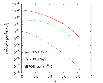
Figure 1: Different contributions to the unpolarized cross section, plotted as a function of $x_{F}$, for $p\,p\to\pi^{0}\,X$ processes and E704 kinematics, as indicated in the plot. The three curves correspond to: solid line = usual unpolarized contribution; dashed line = Boer-Mulders $\otimes$ Collins; dotted line = Boer-Mulders $\otimes$ Boer-Mulders.

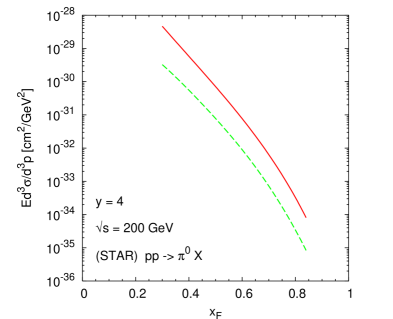
Figure 2: Different contributions to the unpolarized cross section, plotted as a function of $x_{F}$, for $p\,p\to\pi^{0}\,X$ processes and STAR kinematics, as indicated in the plot. The 2 lines correspond to: solid line = usual unpolarized contribution; dashed line = Boer-Mulders $\otimes$ Collins. The Boer-Mulders $\otimes$ Boer-Mulders contribution is not even noticeable at the scale of the figure.

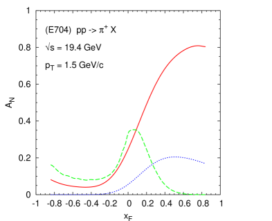
Figure 3: Different contributions to $A_{N}$, plotted as a function of $x_{F}$, for $p^{\uparrow}p\to\pi^{+}\,X$ processes and E704 kinematics. The different lines correspond to: solid line = quark Sivers mechanism alone; dashed line = gluon Sivers mechanism alone; dotted line = transversity $\otimes$ Collins. All other contributions are much smaller.

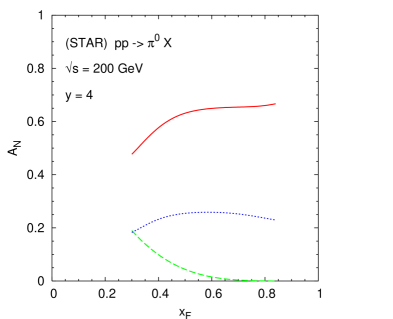
Figure 4: Different contributions to $A_{N}$, plotted as a function of $x_{F}$, for $p^{\uparrow}p\to\pi^{0}\,X$ processes and STAR kinematics. The different lines correspond to: solid line = quark Sivers mechanism alone; dashed line = gluon Sivers mechanism alone; dotted line = transversity $\otimes$ Collins. All other contributions are much smaller.

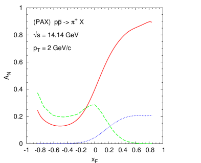
Figure 5: Different contributions to $A_{N}$, plotted as a function of $x_{F}$, for $p^{\uparrow}\bar{p}\to\pi^{+}\,X$ processes and PAX kinematics, as indicated in the plot. The different lines correspond to: solid line = quark Sivers mechanism alone; dashed line = gluon Sivers mechanism alone; dotted line = transversity $\otimes$ Collins. All other contributions are much smaller.

VI Conclusions

We have discussed in great detail a QCD based hard scattering formalism to compute unpolarized and polarized inclusive cross sections for the production of large $p_{T}$ particles in hadronic interactions. In the absence of rigorous results, we have assumed a factorized scheme in which long distance non perturbative physics and short distance pQCD interactions are separated and convoluted; such a factorization has been proven in collinear QCD, but has to be considered as a model when intrinsic motion of partons – effectively introducing higher-twist effects – is allowed for. This is the first study in which the intrinsic $k_{\perp}$ of all participating partons is taken into account. This intrinsic motion of partons, generated both by confinement and QCD dynamics, plays little or no role in unpolarized processes at very large energy, when all relevant momenta are much higher than the average $\langle k_{\perp}\rangle$; it is however crucial in unpolarized processes at intermediate energies fu and, even more so, in the understanding of spin effects and polarized phenomena. For these, partonic spin–$\mbox{\boldmath$k$}_{\perp}$ correlations are of fundamental importance: an ever increasing number of spin experiments and spin measurements is proving that e704 ; star ; herm .

Eq. (I) is our central point; it is essentially a QCD parton model, in which LO (in $\alpha_{s}$) pQCD interactions couple to parton distribution and fragmentation functions; intrinsic motion is fully taken into account in soft physics and in the elementary interactions. As it is well known, this allows new soft partonic functions which would vanish in the collinear limit; however, it also introduces in the hard partonic interactions many $\mbox{\boldmath$k$}_{\perp}$-dependent phases, which strongly affect the convolution of the soft and hard parts. Luckily, it proves that such complicated convolutions involving many phases and many soft functions, have the simplifying result of strongly suppressing most contributions to $(A,S_{A})+(B,S_{B})\to C+X$ inclusive processes. Concerning transverse single spin asymmetries $A_{N}$, this leaves at work essentially only one spin–$\mbox{\boldmath$k$}_{\perp}$ correlation, namely the Sivers mechanism siv . This allows to explain many measured and intriguing values of $A_{N}$ fu ; noidis12 .

We have fully discussed all soft functions, with attention to their physical partonic interpretation, both in terms of polarized distribution and fragmentation functions and in terms of the amplitudes relating partonic and hadronic properties. We have also explicitely shown the exact relationships between different notations widely used in the literature; this should help in understanding and using the $\mbox{\boldmath$k$}_{\perp}$-dependent factorized scheme. Then, we have numerically shown the suppression of many contributions, both to the unpolarized cross section and the SSA $A_{N}$. This confirms and completes the work of Ref. noi .

Many more applications of Eq. (I), modified to hold for different processes, can easily be foreseen. This has been done concerning the Sivers asymmetry in SIDIS processes noidis12 and can be extended to the SIDIS Collins asymmetry noiprep ; single and double spin asymmetries in single particle inclusive production and Drell-Yan processes can equally well be studied, and so on. Some information on Sivers and Collins functions is already available from ongoing experiments herm ; belle and more is expected; a consistent understanding and computation of high energy spin effects, in the framework of a factorized QCD based model, is building up.

Appendix A Detailed $\mbox{\boldmath$k$}_{\perp}$ kinematics

We give here, for completeness and the reader’s convenience, a detailed account of the partonic kinematics with the full inclusion of all transverse momenta, following Refs. cont and fu . As throughout the paper, we consider the hadronic reaction $A\,B\to C\,X$ in the $AB$ center of mass frame with $A$ moving along the positive $Z_{cm}$-axis and we fix the scattering plane as the $(XZ)_{cm}$ plane. We neglect all masses, both the hadronic and the partonic ones.

The 4-momenta of hadrons $A,B,C$ then read

$$p_{A}^{\mu}=\frac{\sqrt{s}}{2}\,(1,\,0,\,0,\,1)\quad\quad p_{B}^{\mu}=\frac{\sqrt{s}}{2}\,(1,\,0,\,0,\,-1)\quad\quad p_{C}^{\mu}=(E_{C},\,p_{T},\,0,\,p_{L})\,,$$ (91)

with $E_{C}=\sqrt{p_{T}^{2}+p_{L}^{2}}$ and $s=(p_{A}+p_{B})^{2}$.

For massless partons $a,b$ inside hadrons $A,B$ we introduce light-cone momentum fractions $x_{a}=p_{a}^{+}/p_{A}^{+}=(p_{a}^{0}+p_{a}^{3})/(p_{A}^{0}+p_{A}^{3})$, $x_{b}=p_{b}^{+}/p_{B}^{+}=(p_{b}^{0}-p_{b}^{3})/(p_{B}^{0}-p_{B}^{3})$ and the transverse momenta $\mbox{\boldmath$k$}_{\perp a}$, $\mbox{\boldmath$k$}_{\perp b}$. Their four-momenta then read

$$p_{a}^{\mu} = x_{a}\,\frac{\sqrt{s}}{2}\left(1+\frac{k_{\perp a}^{2}}{x_{a}^{2}\,s},\>\frac{2k_{\perp a}}{x_{a}\sqrt{s}}\,\cos\phi_{a},\>\frac{2k_{\perp a}}{x_{a}\sqrt{s}}\,\sin\phi_{a},\>1-\frac{k_{\perp a}^{2}}{x_{a}^{2}\,s}\right)$$

$$p_{b}^{\mu} = x_{b}\,\frac{\sqrt{s}}{2}\left(1+\frac{k_{\perp b}^{2}}{x_{b}^{2}\,s},\>\frac{2k_{\perp b}}{x_{b}\sqrt{s}}\,\cos\phi_{b},\>\frac{2k_{\perp b}}{x_{b}\sqrt{s}}\,\sin\phi_{b},\>-1+\frac{k_{\perp b}^{2}}{x_{b}^{2}\,s}\right)\>,$$ (92)

where $k_{\perp a,b}=|\mbox{\boldmath$k$}_{\perp a,b}|$ and $\phi_{a,b}$ are the azimuthal angles of parton $a,b$ three-momenta in the hadronic c.m. frame.

The four-momentum of the fragmenting parton $c$ is given in terms of the observed hadron momentum $p_{C}^{\mu}$, of the light-cone momentum fraction $z=p_{C}^{+}/p_{c}^{+}$ and of the transverse momentum $\mbox{\boldmath$k$}_{\perp C}$ of hadron $C$ with respect to parton $c$ light-cone direction. In the hadronic c.m. frame, we write in general $\mbox{\boldmath$k$}_{\perp C}$ as:

$$\mbox{\boldmath$k$}_{\perp C}=k_{\perp C}\,(\sin\theta_{k_{\perp C}}\cos\phi_{k_{\perp C}},\>\sin\theta_{k_{\perp C}}\sin\phi_{k_{\perp C}},\>\cos\theta_{k_{\perp C}})\,,$$ (93)

and impose the orthogonality condition $\mbox{\boldmath$k$}_{\perp C}\cdot\mbox{\boldmath$p$}_{c}=0$ via the $\delta$-function $\delta(\mbox{\boldmath$k$}_{\perp C}\cdot\hat{\mbox{\boldmath$p$}}_{c})$, where $\hat{\mbox{\boldmath$p$}}_{c}$ is the unit vector along the direction of motion of parton $c$. The parton four-momentum, $p_{c}^{\mu}=(E_{c},\mbox{\boldmath$p$}_{c})$, can then be written as

$$\mbox{\boldmath$p$}_{c} = \frac{E_{c}}{\sqrt{E_{C}^{2}-k_{\perp C}^{2}}}\,(p_{T}-k_{\perp C}\sin\theta_{k_{\perp C}}\cos\phi_{k_{\perp C}},\>-k_{\perp C}\sin\theta_{k_{\perp C}}\sin\phi_{k_{\perp C}},\>p_{L}-k_{\perp C}\cos\theta_{k_{\perp C}})$$

$$E_{c} = \frac{E_{C}+\sqrt{E_{C}^{2}-k_{\perp C}^{2}}}{2z}\>,$$ (94)

and the orthogonality condition $\mbox{\boldmath$k$}_{\perp C}\cdot\mbox{\boldmath$p$}_{c}=0$ implies

$$d^{3}\mbox{\boldmath$k$}_{\perp C}\,\delta(\mbox{\boldmath$k$}_{\perp C}\cdot\hat{\mbox{\boldmath$p$}}_{c}) = k_{\perp C}\,dk_{\perp C}\,d\theta_{k_{\perp C}}\,d\phi_{k_{\perp C}}\,\frac{\sqrt{E_{C}^{2}-k_{\perp C}^{2}}}{p_{T}\,\sin\phi^{0}_{k_{\perp C}}}$$ (95)

$$\times \left[\delta(\phi_{k_{\perp C}}-\phi^{0}_{k_{\perp C}})+\delta(\phi_{k_{\perp C}}-(2\pi-\phi^{0}_{k_{\perp C}}))\right]\,,$$

$$\cos\phi^{0}_{k_{\perp C}} = \frac{k_{\perp C}-p_{L}\cos\theta_{k_{\perp C}}}{p_{T}\sin\theta_{k_{\perp C}}},\;\;0\leq\phi^{0}_{k_{\perp C}}\leq\pi\>.$$ (96)

This allows to perform directly the integration over $\phi_{k_{\perp C}}$ (notice that there are two possible solutions to be considered).

The factor $J(z,k_{\perp C})$ entering our basic factorization formula, Eq. (I), is the Jacobian factor connecting the parton $c$ to hadron $C$ invariant phase space, defined as

$$\frac{d^{3}\bm{p}_{c}}{E_{c}}=\frac{1}{z^{2}}\,J(z,k_{\perp C})\frac{d^{3}\bm{p}_{C}}{E_{C}}\,,$$ (97)

which for collinear and massless particles reduces simply to $J=1$. With intrinsic motion, for massless partons and hadrons:

$$J(z,k_{\perp C})\equiv J(k_{\perp C})=\frac{\left(E_{C}+\sqrt{E_{C}^{2}-k_{\perp C}^{2}}\right)^{2}}{4\,(E_{C}^{2}-k_{\perp C}^{2})}\,\cdot$$ (98)

With the expression of parton momenta given in Eqs. (A) and (94) one can calculate the partonic Mandelstam invariants:

$$\hat{s}=(p_{a}+p_{b})^{2} = x_{a}x_{b}s\left[1-2\frac{k_{\perp a}k_{\perp b}}{x_{a}x_{b}s}\cos(\phi_{a}-\phi_{b})+\frac{k_{\perp a}^{2}k_{\perp b}^{2}}{x_{a}^{2}x_{b}^{2}s^{2}}\right]\,,$$ (99)

$$\hat{t}=(p_{a}-p_{c})^{2} = \frac{T}{z}\,,$$ (100)

$$\hat{u}=(p_{b}-p_{c})^{2} = \frac{U}{z}\,,$$ (101)

$$\hat{s}\,\delta(\hat{s}+\hat{t}+\hat{u}) = z\,\delta\left(z+\frac{T+U}{\hat{s}}\right)\,,$$ (102)

where

$$T = -x_{a}\,\sqrt{s}\,\frac{E_{C}+\sqrt{E_{C}^{2}-k_{\perp C}^{2}}}{2\sqrt{E_{C}^{2}-k_{\perp C}^{2}}}$$ (103)

$$\times \Bigg{\{}\left(1+\frac{k_{\perp a}^{2}}{x_{a}^{2}\,s}\right)\sqrt{E_{C}^{2}-k_{\perp C}^{2}}-\frac{2k_{\perp a}}{x_{a}\sqrt{s}}\>\cos\phi_{a}(p_{T}-k_{\perp C}\sin\theta_{k_{\perp C}}\cos\phi_{k_{\perp C}})$$

$$+ \frac{2k_{\perp a}}{x_{a}\sqrt{s}}\>k_{\perp C}\,\sin\phi_{a}\sin\theta_{k_{\perp C}}\sin\phi_{k_{\perp C}}-\left(1-\frac{k_{\perp a}^{2}}{x_{a}^{2}\,s}\right)(p_{L}-k_{\perp C}\cos\theta_{k_{\perp C}})\Bigg{\}}$$

$$U = -x_{b}\,\sqrt{s}\,\frac{E_{C}+\sqrt{E_{C}^{2}-k_{\perp C}^{2}}}{2\sqrt{E_{C}^{2}-k_{\perp C}^{2}}}$$ (104)

$$\times \Bigg{\{}\left(1+\frac{k_{\perp b}^{2}}{x_{b}^{2}\,s}\right)\sqrt{E_{C}^{2}-k_{\perp C}^{2}}-\frac{2k_{\perp b}}{x_{b}\sqrt{s}}\>\cos\phi_{b}(p_{T}-k_{\perp C}\sin\theta_{k_{\perp C}}\cos\phi_{k_{\perp C}})$$

$$+ \frac{2k_{\perp b}}{x_{b}\sqrt{s}}\>k_{\perp C}\,\sin\phi_{b}\sin\theta_{k_{\perp C}}\sin\phi_{k_{\perp C}}+\left(1-\frac{k_{\perp b}^{2}}{x_{b}^{2}\,s}\right)(p_{L}-k_{\perp C}\cos\theta_{k_{\perp C}})\Bigg{\}}\>.$$

The phase space integrations must obey some constraints, originating from physical requests. Besides the trivial bounds $0<x_{a,b},z<1$, $0\leq\phi_{a,b}\leq 2\pi$ and $0\leq\theta_{k_{\perp C}}\leq\pi$, we require that, even including intrinsic transverse momentum effects, $a)$ each parton keeps moving along the same direction as its parent hadron, $\mbox{\boldmath$p$}_{a(b)}\cdot\mbox{\boldmath$P$}_{A(B)}>0$, and $b)$ the parton energy is not larger than the parent hadron energy, $E_{a(b)}\leq E_{A(B)}$. This implies the following bounds

$$k_{\perp a(b)}/\sqrt{s}<\min\left[x_{a(b)},\>\sqrt{x_{a(b)}(1-x_{a(b)})}\right]\>.$$ (105)

Analogously, for the fragmentation process $c\to C+X$ we require $\mbox{\boldmath$p$}_{c}\cdot\mbox{\boldmath$P$}_{C}>0$ and $E_{C}\leq E_{c}$ (both fulfilled by Eq. (94), where we have consistently disregarded the solution $E_{c}=\left[E_{C}-\sqrt{E_{C}^{2}-k_{\perp C}^{2}}\right]/(2z)$). The last constraint implies the following bound on $k_{\perp C}$, at fixed $z$ values:

$$k_{\perp C}/E_{C}\leq 1\;\,(z\leq 1/2)\quad\quad k_{\perp C}/E_{C}\leq 2\sqrt{z(1-z)}\;\,(z>1/2)\>.$$ (106)

By requiring $|\cos\phi^{0}_{k_{\perp C}}|\leq 1$, see Eq. (96), we have a further constraint on $k_{\perp C}$, at fixed $\theta_{k_{\perp C}}$, namely

$$p_{L}\cos\theta_{k_{\perp C}}-p_{T}\sin\theta_{k_{\perp C}}\leq k_{\perp C}\leq p_{L}\cos\theta_{k_{\perp C}}+p_{T}\sin\theta_{k_{\perp C}}\>.$$ (107)

The partonic helicity amplitudes are computed according to Eqs. (59)–(61); the explicit expressions, in terms of the Mandelstam variables, of the relevant combinations of the $\hat{M}^{0}$ amplitudes are given in Section III of the text. The phases $\varphi_{i}$ are defined in Eq. (61). For processes involving only quarks and antiquarks they read:

$$\varphi_{1} = -\frac{1}{2}\left(\xi_{a}+\xi_{b}-\xi_{c}-\xi_{d}\right)$$

$$\varphi_{2} = \frac{1}{2}\left(\xi_{a}-\xi_{b}-\xi_{c}+\xi_{d}\right)+\tilde{\xi}_{a}-\tilde{\xi}_{c}-\phi^{\prime\prime}_{c}$$ (108)

$$\varphi_{3} = \frac{1}{2}\left(-\xi_{a}+\xi_{b}-\xi_{c}+\xi_{d}\right)-\tilde{\xi}_{a}-\tilde{\xi}_{c}+\phi^{\prime\prime}_{c}\>.$$

Similarly for processes involving also gluons.

All terms appearing in the above phases are discussed and can be found in Ref. noi ; we report them here for convenience and self-consistency of the paper:

$$\cos\xi_{j} = \frac{\cos\theta_{q}\sin\theta_{j}-\sin\theta_{q}\cos\theta_{j}\cos(\phi_{q}-\phi_{j})}{\sin\theta_{qp_{j}}}$$ (109)

$$\sin\xi_{j} = \frac{\sin\theta_{q}\sin(\phi_{q}-\phi_{j})}{\sin\theta_{qp_{j}}}\>\cdot$$ (110)

All angles refer to the overall $AB$ c.m. frame. $\theta_{j}$ and $\phi_{j}$ ($j=a,b,c,d$) are respectively the polar and azimuthal angles of the partons, while $\theta_{q}$ and $\phi_{q}$ are the polar and azimuthal angle of the vector $\mbox{\boldmath$q$}=\mbox{\boldmath$p$}_{a}+\mbox{\boldmath$p$}_{b}$. Here and in the next equations $\theta_{qp_{j}}$ ($0\leq\theta_{qp_{j}}\leq\pi$) denotes in general the angle between the two vectors $q$ and $\mbox{\boldmath$p$}_{j}$.

The $\tilde{\xi}_{j}$ angles ($j=a,b,c,d$) are given by

$$\tilde{\xi}_{j}=\eta^{\prime}_{j}+\xi^{\prime}_{j}\>,$$ (111)

where

$$\cos\xi^{\prime}_{j} = \frac{\cos\theta_{q}\sin\theta^{\prime}_{j}-\sin\theta_{q}\cos\theta^{\prime}_{j}\cos(\phi_{q}-\phi^{\prime}_{j})}{\sin\theta_{qp^{\prime}_{j}}}$$ (112)

$$\sin\xi^{\prime}_{j} = \frac{-\sin\theta_{q}\sin(\phi_{q}-\phi^{\prime}_{j})}{\sin\theta_{qp^{\prime}_{j}}}\>;$$ (113)

$$\cos\eta^{\prime}_{j} = \frac{\cos\theta^{\prime}_{a}-\cos\theta^{\prime}_{j}\cos\theta_{p^{\prime}_{a}p^{\prime}_{j}}}{\sin\theta^{\prime}_{j}\sin\theta_{p^{\prime}_{a}p^{\prime}_{j}}}$$ (114)

$$\sin\eta^{\prime}_{j} = \frac{\sin\theta^{\prime}_{a}\sin(\phi^{\prime}_{a}-\phi^{\prime}_{j})}{\sin\theta_{p^{\prime}_{a}p^{\prime}_{j}}}\>\cdot$$ (115)

The primed angles $(\theta^{\prime}_{j},\phi^{\prime}_{j})$ are obtained via

$$\mbox{\boldmath$p$}_{i}^{\prime}=\mbox{\boldmath$p$}_{i}-\frac{\bm{q}}{q^{0}+\sqrt{q^{2}}}\left(\frac{p_{i}\cdot q}{\sqrt{q^{2}}}+p_{i}^{0}\right)$$ (116)

where $i=a,b,c,d$ and $q^{\mu}=(q^{0},\bm{q})=p_{a}^{\mu}+p_{b}^{\mu}$.

The last angle appearing in Eqs. (108) is $\phi^{\prime\prime}_{c}$, given by:

$$\tan\phi^{\prime\prime}_{c}=\frac{\sin\theta^{\prime}_{c}\sin(\phi^{\prime}_{c}-\phi^{\prime}_{a})}{\sin\theta^{\prime}_{c}\cos(\phi^{\prime}_{c}-\phi^{\prime}_{a})\cos\theta^{\prime}_{a}-\cos\theta^{\prime}_{c}\sin\theta^{\prime}_{a}}\,\cdot$$ (117)

Finally, the angle $\phi^{H}_{C}$ appearing in the fragmentation amplitudes, Eq. (45), is given, in terms of our integration and overall variables, by:

$$\tan\phi^{H}_{C}=\mp\frac{p_{T}}{\sqrt{E^{2}_{C}-k^{2}_{\perp C}}}\,\sqrt{1-\left(\frac{k_{\perp C}-p_{L}\cos\theta_{k_{\perp C}}}{p_{T}\sin\theta_{k_{\perp C}}}\right)^{2}}\,\tan\theta_{k_{\perp C}}\,,$$ (118)

where the $\mp$ signs refer, respectively, to the first and second $\delta$-function terms in Eq. (95).

Appendix B Parton polarizations and distribution amplitudes

An alternative simple physical interpretation can be given to the distribution functions $(P^{a}_{j}\hat{f}_{a/A,S_{A}})=\Delta\hat{f}^{a}_{s_{j}/S_{A}}$ by making use of the helicity amplitudes ${\hat{\cal F}}_{\lambda^{\,}_{a},\lambda^{\,}_{X_{A}};\lambda^{\,}_{A}}$, which describe the soft process $A\to a+X$. This is the approach used in Refs. noi ; noi95 . Since the partonic distribution is usually regarded, at LO, as the inclusive cross section for this process, the helicity density matrix of parton $a$ inside hadron $A$ with spin $S_{A}$ and polarization vector $\mbox{\boldmath$P$}^{A}$ can be written as

$$\rho_{\lambda^{\,}_{a},\lambda^{\prime}_{a}}^{a/A,S_{A}}\>\hat{f}_{a/A,S_{A}}(x_{a},\mbox{\boldmath$k$}_{\perp a}) = \sum_{\lambda^{\,}_{A},\lambda^{\prime}_{A}}\rho_{\lambda^{\,}_{A},\lambda^{\prime}_{A}}^{A,S_{A}}\mathrel{\mathop{\kern 0.0pt\hbox to0.0pt{\hbox{$\sum$}\hss}}\hbox{\kern-1.25pt$\displaystyle\int$}}_{X_{A},\lambda_{X_{A}}}\!\!\!\!\!{\hat{\cal F}}_{\lambda^{\,}_{a},\lambda^{\,}_{X_{A}};\lambda^{\,}_{A}}\,{\hat{\cal F}}^{*}_{\lambda^{\prime}_{a},\lambda^{\,}_{X_{A}};\lambda^{\prime}_{A}}$$ (119)

$$\equiv \sum_{\lambda^{\,}_{A},\lambda^{\prime}_{A}}\rho_{\lambda^{\,}_{A},\lambda^{\prime}_{A}}^{A,S_{A}}\>\hat{F}_{\lambda^{\,}_{A},\lambda^{\prime}_{A}}^{\lambda^{\,}_{a},\lambda^{\prime}_{a}}\>,$$

having defined

$$\hat{F}_{\lambda^{\,}_{A},\lambda^{\prime}_{A}}^{\lambda^{\,}_{a},\lambda^{\prime}_{a}}\equiv\>\mathrel{\mathop{\kern 0.0pt\hbox to0.0pt{\hbox{$\sum$}\hss}}\hbox{\kern-1.25pt$\displaystyle\int$}}_{X_{A},\lambda_{X_{A}}}\!\!\!\!\!\!{\hat{\cal F}}_{\lambda^{\,}_{a},\lambda^{\,}_{X_{A}};\lambda^{\,}_{A}}\,{\hat{\cal F}}^{*}_{\lambda^{\prime}_{a},\lambda^{\,}_{X_{A}};\lambda^{\prime}_{A}}\>,$$ (120)

where the $\mathrel{\mathop{\kern 0.0pt\hbox to0.0pt{\hbox{$\sum$}\hss}}\hbox{\kern-1.25pt$\displaystyle\int$}}_{X_{A},\lambda_{X_{A}}}\!\!\!$ stands for a spin sum and phase space integration over all undetected remnants of hadron $A$, considered as a system $X_{A}$, and the $\hat{\cal F}$’s are the helicity distribution amplitudes for the $A\to a+X$ process.

Eq. (119) relates the helicity density matrix of parton $a$, see Eq. (7), to the helicity density matrix of hadron $A$, given by

$$\rho_{\lambda^{\,}_{A},\lambda^{\prime}_{A}}^{A,S_{A}}=\frac{1}{2}\,{\left(\begin{array}[]{cc}1+P^{A}_{Z}&P^{A}_{X}-iP^{A}_{Y}\\ P^{A}_{X}+iP^{A}_{Y}&1-P^{A}_{Z}\end{array}\right)}_{\!\!\!A,S_{A}}=\frac{1}{2}\,{\left(\begin{array}[]{cc}1+P^{A}_{L}&P^{A}_{T}\,e^{-i\phi_{S_{A}}}\\ P^{A}_{T}\,e^{i\phi_{S_{A}}}&1-P^{A}_{L}\end{array}\right)}_{\!\!\!A,S_{A}}\,,$$ (121)

where $\mbox{\boldmath$P$}^{A}=(P^{A}_{T}\cos\phi_{S_{A}},P^{A}_{T}\sin\phi_{S_{A}},P^{A}_{L})$ is hadron $A$ polarization vector and $\phi_{S_{A}}$ its azimuthal angle, defined in the helicity reference frame of hadron $A$. Notice that, in this Appendix, we consider the most general case in which the transverse polarization of hadron $A$ can be along any direction $\phi_{S_{A}}$ in the $XY$ plane, whereas in Section II.1 and throughout the paper the specific choice was made of fixing the transverse polarization of hadron $A$ along the $Y$-axis, i.e. $\uparrow\;=S_{Y}$, which corresponds to $\phi_{S_{A}}=\pi/2$.

The distribution amplitudes $\hat{\cal F}$ depend on the parton light-cone momentum fraction $x_{a}$ and on its intrinsic transverse momentum $\mbox{\boldmath$k$}_{\perp a}$, with modulus $k_{\perp a}$ and azimuthal angle $\phi_{a}$:

$$\hat{\cal F}_{\lambda^{\,}_{a},\lambda^{\,}_{X_{A}};\lambda^{\,}_{A}}(x_{a},\mbox{\boldmath$k$}_{\perp a})={\cal F}_{\lambda^{\,}_{a},\lambda^{\,}_{X_{A}};\lambda^{\,}_{A}}(x_{a},k_{\perp a})\>{\rm exp}[i\lambda^{\,}_{A}\phi_{a}]\>,$$ (122)

so that

$$\hat{F}_{\lambda^{\,}_{A},\lambda^{\prime}_{A}}^{\lambda^{\,}_{a},\lambda^{\prime}_{a}}(x_{a},\mbox{\boldmath$k$}_{\perp a})=F_{\lambda^{\,}_{A},\lambda^{\prime}_{A}}^{\lambda^{\,}_{a},\lambda^{\prime}_{a}}(x_{a},k_{\perp a})\>{\rm exp}[i(\lambda^{\,}_{A}-\lambda^{\prime}_{A})\phi_{a}]\>.$$ (123)

$F_{\lambda^{\,}_{A},\lambda^{\prime}_{A}}^{\lambda^{\,}_{a},\lambda^{\prime}_{a}}(x_{a},k_{\perp a})$ has the same definition as $\hat{F}_{\lambda^{\,}_{A},\lambda^{\prime}_{A}}^{\lambda^{\,}_{a},\lambda^{\prime}_{a}}(x_{a},\mbox{\boldmath$k$}_{\perp a})$, Eq. (120), with $\hat{\cal F}$ replaced by ${\cal F}$, and does not depend on phases anymore.

The parity properties of ${\cal F}_{\lambda^{\,}_{a},\lambda^{\,}_{X_{A}};\lambda^{\,}_{A}}(x_{a},k_{\perp a})$ are the usual ones valid for helicity amplitudes in the $\phi_{a}=0$ plane elliot ,

$${\cal F}_{-\lambda^{\,}_{a},-\lambda^{\,}_{X_{A}};-\lambda^{\,}_{A}}=\eta\,(-1)^{S_{A}-s_{a}-S_{X_{A}}}\>(-1)^{\lambda^{\,}_{A}-\lambda^{\,}_{a}+\lambda^{\,}_{X_{A}}}\>{\cal F}_{\lambda^{\,}_{a},\lambda^{\,}_{X_{A}};\lambda^{\,}_{A}}\>,$$ (124)

where $\eta$ is an intrinsic parity factor such that $\eta^{2}=1$. These imply:

$${F}_{-\lambda^{\,}_{A},-\lambda^{\prime}_{A}}^{-\lambda^{\,}_{a},-\lambda^{\prime}_{a}}=(-1)^{2(S_{A}-s_{a})}\>(-1)^{(\lambda^{\,}_{A}-\lambda^{\,}_{a})+(\lambda^{\prime}_{A}-\lambda^{\prime}_{a})}\>{F}_{\lambda^{\,}_{A},\lambda^{\prime}_{A}}^{\lambda^{\,}_{a},\lambda^{\prime}_{a}}\,.$$ (125)

Notice that, for $S_{A}=1/2$, the factor $(-1)^{2(S_{A}-s_{a})}$ is positive if parton $a$ is a quark and negative if it is a gluon; consequently, some parity relations are different according to the nature of the parton involved. For this reason we shall treat quark and gluon distribution functions separately.

By applying Eqs. (123) and (125) one can see that there are six independent $F$’s:

$$F^{++}_{++}\,,\,\,F^{++}_{--}\,,\,\,F^{+-}_{+-}\,,\,\,F^{-+}_{+-}\,,\,F^{++}_{+-}\,,\,\,F^{+-}_{++}\,.$$ (126)

These are in principle complex quantities, but $F^{++}_{++}$ and $F^{++}_{--}$ are clearly moduli squared (see Eq. 120), whereas $F^{+-}_{+-}$ and $F^{-+}_{+-}$ are purely imaginary for gluons and purely real for quarks, as given by Eq. (125). This leaves us with eight independent real quantities, which are directly related to the eight distribution functions defined in Eqs. (13-15) (for quarks) and (29-35) (for gluons), as we are going to show.

B.1 Quark sector

Let us consider first quark partons. Inserting Eqs. (121) and (123) into Eq. (119), and exploiting the parity relationships (125), yields, for a generic hadronic spin state:

$$\rho^{a/A,S_{A}}_{++}\hat{f}_{a/A,S_{A}} = \frac{1}{2}\,(1+P_{z}^{a})\,\hat{f}_{a/A,S_{A}}=\frac{1}{2}\left(F^{++}_{++}+F^{++}_{--}\right)+\frac{1}{2}\,P_{L}^{A}\left(F^{++}_{++}-F^{++}_{--}\right)$$ (127)

$$+ P_{T}^{A}\,\left[{\rm Re}F^{++}_{+-}\,\cos(\phi_{S_{A}}-\phi_{a})+{\rm Im}F^{++}_{+-}\,\sin(\phi_{S_{A}}-\phi_{a})\right]$$

$$\rho^{a/A,S_{A}}_{--}\hat{f}_{a/A,S_{A}} = \frac{1}{2}\,(1-P_{z}^{a})\,\hat{f}_{a/A,S_{A}}=\frac{1}{2}\left(F^{++}_{++}+F^{++}_{--}\right)-\frac{1}{2}\,P_{L}^{A}\left(F^{++}_{++}-F^{++}_{--}\right)$$ (128)

$$- P_{T}^{A}\,\left[{\rm Re}F^{++}_{+-}\,\cos(\phi_{S_{A}}-\phi_{a})-{\rm Im}F^{++}_{+-}\,\sin(\phi_{S_{A}}-\phi_{a})\right]$$

$$\rho^{a/A,S_{A}}_{+-}\hat{f}_{a/A,S_{A}}=\frac{1}{2}\,(P^{a}_{x}-iP_{y}^{a})\,\hat{f}_{a/A,S_{A}}=i\,{\rm Im}F^{+-}_{++}\,+\,P_{L}^{A}\,{\rm Re}F^{+-}_{++}$$

$$\>\>\>\>+\>\frac{1}{2}\,P_{T}^{A}\left[\left(F^{+-}_{+-}+F^{-+}_{+-}\right)\cos(\phi_{S_{A}}-\phi_{a})-i\,\left(F^{+-}_{+-}-F^{-+}_{+-}\right)\sin(\phi_{S_{A}}-\phi_{a})\right]\,.$$ (129)

By summing and subtracting Eqs. (127) and (128), one finds

$$\hat{f}_{a/A,S_{A}}=\left(F^{++}_{++}+F^{++}_{--}\right)+2\,P_{T}^{A}\,{\rm Im}F^{++}_{+-}\sin(\phi_{S_{A}}-\phi_{a})$$ (130)

$$P_{z}^{a}\,\hat{f}_{a/A,S_{A}}=P_{L}^{A}\left(F^{++}_{++}-F^{++}_{--}\right)+2\,P_{T}^{A}\,{\rm Re}F^{++}_{+-}\cos(\phi_{S_{A}}-\phi_{a})\>,$$ (131)

while from the real and imaginary parts of Eq. (129),

$$P_{x}^{a}\,\hat{f}_{a/A,S_{A}} = 2\,P^{A}_{L}\,{\rm Re}F^{+-}_{++}+P_{T}^{A}\,\left(F^{+-}_{+-}+F^{-+}_{+-}\right)\,\cos(\phi_{S_{A}}-\phi_{a})$$ (132)

$$P_{y}^{a}\,\hat{f}_{a/A,S_{A}} = -2\,{\rm Im}F^{+-}_{++}+P_{T}^{A}\,\left(F^{+-}_{+-}-F^{-+}_{+-}\right)\,\sin(\phi_{S_{A}}-\phi_{a})\>.$$ (133)

The two above equations can be written in a compact form (which we shall use later) in terms of the parton transverse spin

$$P_{x}^{a}=P^{a}_{T}\cos\phi_{s_{a}}\quad\quad\quad P_{y}^{a}=P^{a}_{T}\sin\phi_{s_{a}},$$ (134)

where $\phi_{s_{a}}$ is the azimuthal angle of the polarization vector of parton $a$ in its helicity frame. By multiplying Eqs. (132) and (133) respectively by $\cos\phi_{s_{a}}$ and $\sin\phi_{s_{a}}$ and summing, one obtains:

$$P^{a}_{T}\hat{f}_{a/A,S_{A}} = -2\,{\rm Im}F^{+-}_{++}\sin\phi_{s_{a}}+2\,P^{A}_{L}\,{\rm Re}F^{+-}_{++}\cos\phi_{s_{a}}$$ (135)

$$+\;P_{T}^{A}\,\left[F^{+-}_{+-}\cos(\phi_{s_{a}}-\phi_{S_{A}}+\phi_{a})+F^{-+}_{+-}\cos(\phi_{s_{a}}+\phi_{S_{A}}-\phi_{a})\right]\,.$$

Moreover, one can show that the azimuthal angle of $\mbox{\boldmath$P$}^{a}$ in its helicity frame, $\phi_{s_{a}}$, and the same angle measured in the hadronic helicity frame, $\phi^{\prime}_{s_{a}}$, are related by

$$\phi_{s_{a}}=\phi^{\prime}_{s_{a}}-\phi_{a}+{\cal O}\left(\left[\frac{k_{\perp a}}{x_{a}\sqrt{s}}\right]^{2}\right)\>,$$ (136)

so that, up to such corrections, Eq. (135) can be written as

$$P^{a}_{T}\hat{f}_{a/A,S_{A}} = -2\,{\rm Im}F^{+-}_{++}\sin(\phi^{\prime}_{s_{a}}-\phi_{a})+2\,P^{A}_{L}\,{\rm Re}F^{+-}_{++}\cos(\phi^{\prime}_{s_{a}}-\phi_{a})$$ (137)

$$+\;P_{T}^{A}\,\left[F^{+-}_{+-}\cos(\phi^{\prime}_{s_{a}}-\phi_{S_{A}})+F^{-+}_{+-}\cos(\phi^{\prime}_{s_{a}}+\phi_{S_{A}}-2\phi_{a})\right]\,.$$

Eqs. (130)-(133) express the quark polarizations in term of the distribution amplitudes $F$’s and the hadron polarization. One finds eight non zero independent soft functions:

$$\hat{f}_{a/A} = \hat{f}_{a/A,S_{L}}=\left(F^{++}_{++}+F^{++}_{--}\right)$$ (138)

$$\hat{f}_{a/A,S_{T}} = \left(F^{++}_{++}+F^{++}_{--}\right)+2\,{\rm Im}F^{++}_{+-}\sin(\phi_{S_{A}}-\phi_{a})$$ (139)

$$P_{x}^{a}\,\hat{f}_{a/A,S_{L}} = 2\,{\rm Re}F^{+-}_{++}$$ (140)

$$P_{x}^{a}\,\hat{f}_{a/A,S_{T}} = \left(F^{+-}_{+-}+F^{-+}_{+-}\right)\,\cos(\phi_{S_{A}}-\phi_{a})$$ (141)

$$P_{y}^{a}\,\hat{f}_{a/A,S_{L}} = P_{y}^{a}\,\hat{f}_{a/A}=-2\,{\rm Im}F^{+-}_{++}$$ (142)

$$P_{y}^{a}\,\hat{f}_{a/A,S_{T}} = -2\,{\rm Im}F^{+-}_{++}+\left(F^{+-}_{+-}-F^{-+}_{+-}\right)\,\sin(\phi_{S_{A}}-\phi_{a})$$ (143)

$$P_{z}^{a}\,\hat{f}_{a/A,S_{L}} = \left(F^{++}_{++}-F^{++}_{--}\right)$$ (144)

$$P_{z}^{a}\,\hat{f}_{a/A,S_{T}} = 2\,{\rm Re}F^{++}_{+-}\cos(\phi_{S_{A}}-\phi_{a})\,.$$ (145)

Notice also that $P_{x}^{a}\,\hat{f}_{a/A}=0$.

If we fix $\phi_{S_{A}}=\pi/2$ as done throughout the paper and adopt the notations of Eqs. (13)-(15), the above equations read:

$$P_{x}^{a}\,\hat{f}_{a/A,S_{Y}} = \Delta\hat{f}_{{s_{x}}/S_{Y}}\equiv\Delta\hat{f}_{{s_{x}}/\uparrow}=\left(F^{+-}_{+-}+F^{-+}_{+-}\right)\sin\phi_{a}$$ (146)

$$P_{y}^{a}\,\hat{f}_{a/A,S_{Y}} = \Delta\hat{f}_{{s_{y}}/S_{Y}}\equiv\Delta\hat{f}_{{s_{y}}/\uparrow}=-2\,{\rm Im}F^{+-}_{++}+\left(F^{+-}_{+-}-F^{-+}_{+-}\right)\cos\phi_{a}$$ (147)

$$P_{z}^{a}\,\hat{f}_{a/A,S_{Y}} = \Delta\hat{f}_{{s_{z}}/S_{Y}}\equiv\Delta\hat{f}_{s_{z}/\uparrow}=2\,{\rm Re}F^{++}_{+-}\sin\phi_{a}$$ (148)

$$P_{x}^{a}\,\hat{f}_{a/A,S_{Z}} = \Delta\hat{f}_{{s_{x}}/S_{Z}}\equiv\Delta\hat{f}_{{s_{x}}/+}=2\,{\rm Re}F^{+-}_{++}$$ (149)

$$P_{y}^{a}\,\hat{f}_{a/A,S_{Z}} = \Delta\hat{f}_{{s_{y}}/S_{Z}}\equiv\Delta\hat{f}_{{s_{y}}/+}=\Delta\hat{f}_{{s_{y}}/A}=-2\,{\rm Im}F^{+-}_{++}$$ (150)

$$P_{z}^{a}\,\hat{f}_{a/A,S_{Z}} = \Delta\hat{f}_{{s_{z}}/S_{Z}}\equiv\Delta\hat{f}_{{s_{z}}/+}=\left(F^{++}_{++}-F^{++}_{--}\right)$$ (151)

$$\hat{f}_{a/A,S_{Y}} = \hat{f}_{a/A}+\frac{1}{2}\,\Delta\hat{f}_{a/S_{Y}}=\left(F^{++}_{++}+F^{++}_{--}\right)+2\,{\rm Im}F^{++}_{+-}\cos\phi_{a}\,,$$ (152)

which gives the exact expressions of Eqs. (13)–(15) in terms of helicity distribution amplitudes. In particular, Eqs. (150) and (152) allow to obtain the expressions of the Boer-Mulders and Sivers functions respectively [see Eqs. (15), (17) and (21)]:

$$\Delta^{N}\hat{f}_{a^{\uparrow}/A} = -2\,{\rm Im}F^{+-}_{++}$$ (153)

$$\Delta^{N}\hat{f}_{a/A^{\uparrow}} = 4\,{\rm Im}F^{++}_{+-}\>.$$ (154)

Notice also that:

$$\Delta^{-}\hat{f}^{a}_{s_{y}/S_{Y}}\equiv\frac{1}{2}\,\left[\Delta\hat{f}^{a}_{s_{y}/\uparrow}-\Delta\hat{f}^{a}_{s_{y}/\downarrow}\right]=\left(F^{+-}_{+-}-F^{-+}_{+-}\right)\cos\phi_{a}\>.$$ (155)

B.2 Gluon sector

Thanks to the formal analogy between Eqs. (7) and (24) the expressions of the circular and linear polarizations of the gluons in terms of the corresponding helicity distribution amplitudes are closely analogous to those obtained for quarks in the previous subsection. One should only pay attention to the parity properties appropriate for spin 1 gluons and remember that the $F$’s are now the helicity distribution amplitudes for the $A\to g+X$ process.

One finds that Eqs. (127) and (128) hold true also for gluons, while Eq. (129), due to the different parity relationships, changes into:

$$\rho^{g/A,S_{A}}_{+-}\hat{f}_{g/A,S_{A}}=\frac{1}{2}(\mathcal{T}_{1}^{g}-i\mathcal{T}_{2}^{g})\hat{f}_{g/A,S_{A}}={\rm Re}F^{+-}_{++}\,+\,i\,P_{L}^{A}\,{\rm Im}F^{+-}_{++}$$

$$\>\>\>-\,\frac{i}{2}\,P_{T}^{A}\left[(F^{+-}_{+-}+F^{-+}_{+-})\sin(\phi_{S_{A}}-\phi_{a})+\,i\,(F^{+-}_{+-}-F^{-+}_{+-})\cos(\phi_{S_{A}}-\phi_{a})\right]\,,$$ (156)

where $F^{+-}_{+-}$ and $F^{-+}_{+-}$ are now purely imaginary quantities.

As a consequence, Eqs. (130) and (131) keep describing the distributions of unpolarized or longitudinally polarized gluons inside a polarized hadron, while Eqs. (132) and (133) modify into:

$$\mathcal{T}_{1}^{g}\hat{f}_{g/A,S_{A}} = 2\,{\rm Re}F_{++}^{+-}+P_{T}^{A}\,{\rm Im}\left(F_{+-}^{+-}+F_{+-}^{-+}\right)\,\sin(\phi_{S_{A}}-\phi_{a})$$ (157)

$$\mathcal{T}_{2}^{g}\hat{f}_{g/A,S_{A}} = -2\,P_{L}^{A}\,{\rm Im}F_{++}^{+-}-P_{T}^{A}\,{\rm Im}\left(F_{+-}^{+-}-F_{+-}^{-+}\right)\,\cos(\phi_{S_{A}}-\phi_{a})\,.$$ (158)

Eqs. (138)–(145) now become:

$$\hat{f}_{g/A} = \hat{f}_{g/A,S_{L}}=\left(F^{++}_{++}+F^{++}_{--}\right)$$ (159)

$$\hat{f}_{g/A,S_{T}} = \left(F^{++}_{++}+F^{++}_{--}\right)+2\,{\rm Im}F^{++}_{+-}\sin(\phi_{S_{A}}-\phi_{a})$$ (160)

$$\mathcal{T}_{1}^{g}\,\hat{f}_{g/A,S_{L}} = \mathcal{T}_{1}^{g}\,\hat{f}_{g/A}=2\,{\rm Re}F^{+-}_{++}$$ (161)

$$\mathcal{T}_{1}^{g}\,\hat{f}_{g/A,S_{T}} = 2\,{\rm Re}F^{+-}_{++}+{\rm Im}\left(F^{+-}_{+-}+F^{-+}_{+-}\right)\,\sin(\phi_{S_{A}}-\phi_{a})$$ (162)

$$\mathcal{T}_{2}^{g}\,\hat{f}_{g/A,S_{L}} = -2\,{\rm Im}F^{+-}_{++}$$ (163)

$$\mathcal{T}_{2}^{g}\,\hat{f}_{g/A,S_{T}} = -\,{\rm Im}\left(F^{+-}_{+-}-F^{-+}_{+-}\right)\,\cos(\phi_{S_{A}}-\phi_{a})$$ (164)

$$P_{z}^{g}\,\hat{f}_{g/A,S_{L}} = \left(F^{++}_{++}-F^{++}_{--}\right)$$ (165)

$$P_{z}^{g}\,\hat{f}_{g/A,S_{T}} = 2\,{\rm Re}F^{++}_{+-}\cos(\phi_{S_{A}}-\phi_{a})\>,$$ (166)

while, choosing $\phi_{S_{A}}=\pi/2$ and following the notation of Eqs. (29)–(35), we have:

$$\mathcal{T}_{1}^{g}\,\hat{f}_{g/A,S_{Y}} = \Delta\hat{f}_{\mathcal{T}_{1}/S_{Y}}^{g}=\Delta\hat{f}_{{\mathcal{T}_{1}}/\uparrow}^{g}=2\,{\rm Re}F^{+-}_{++}+{\rm Im}\left(F^{+-}_{+-}+F^{-+}_{+-}\right)\cos\phi_{a}$$ (167)

$$\mathcal{T}_{2}^{g}\,\hat{f}_{g/A,S_{Y}} = \Delta\hat{f}_{\mathcal{T}_{2}/S_{Y}}^{g}=\Delta\hat{f}_{{\mathcal{T}_{2}}/\uparrow}^{g}=-{\rm Im}\left(F^{+-}_{+-}-F^{-+}_{+-}\right)\sin\phi_{a}$$ (168)

$$P_{z}^{g}\,\hat{f}_{g/A,S_{Y}} = \Delta\hat{f}_{s_{z}/S_{Y}}^{g}=\Delta\hat{f}_{{s_{z}}/\uparrow}^{g}=2\,{\rm Re}F^{++}_{+-}\sin\phi_{a}$$ (169)

$$\mathcal{T}_{1}^{g}\,\hat{f}_{g/A,S_{Z}} = \Delta\hat{f}_{\mathcal{T}_{1}/S_{Z}}^{g}=\Delta\hat{f}_{\mathcal{T}_{1}/+}^{g}=\Delta\hat{f}_{\mathcal{T}_{1}/A}^{g}=2\,{\rm Re}F^{+-}_{++}$$ (170)

$$\mathcal{T}_{2}^{g}\,\hat{f}_{g/A,S_{Z}} = \Delta\hat{f}_{\mathcal{T}_{2}/S_{Z}}^{g}=\Delta\hat{f}_{\mathcal{T}_{2}/+}^{g}=-2\,{\rm Im}F^{+-}_{++}$$ (171)

$$P_{z}^{g}\,\hat{f}_{g/A,S_{Z}} = \Delta\hat{f}_{s_{z}/S_{Z}}^{g}=\Delta\hat{f}_{{s_{z}}/+}^{g}=\left(F^{++}_{++}-F^{++}_{--}\right)$$ (172)

$$\hat{f}_{g/A,S_{Y}} = \hat{f}_{g/A}+\frac{1}{2}\,\Delta\hat{f}_{g/\uparrow}=\left(F^{++}_{++}+F^{++}_{--}\right)+2\,{\rm Im}F^{++}_{+-}\cos\phi_{a}\,.$$ (173)

The Sivers function (154) can exist also for gluons, while the “Boer-Mulders-like” function is given by

$$\mathcal{T}_{1}^{g}\hat{f}_{g/A}=\Delta\hat{f}_{\mathcal{T}_{1}/A}^{g}=\Delta\hat{f}_{\mathcal{T}_{1}/+}^{g}=2\,{\rm Re}F^{+-}_{++}\>.$$ (174)

Finally, in analogy to Eq. (155):

$$\Delta^{-}\hat{f}^{g}_{\mathcal{T}_{1}/S_{Y}}\equiv\frac{1}{2}\,\left[\Delta\hat{f}^{g}_{\mathcal{T}_{1}/\uparrow}-\Delta\hat{f}^{g}_{\mathcal{T}_{1}/\downarrow}\right]={\rm Im}\left(F^{+-}_{+-}+F^{-+}_{+-}\right)\cos\phi_{a}\>.$$ (175)

Appendix C Relations between different notations

C.1 Quark distribution functions

Let us compare our notations with those used in the formalism of the Amsterdam group amst (see also Ref. brd ), which is widely used. In this formalism the main object, corresponding to our $\hat{F}_{\lambda^{\,}_{A},\lambda^{\prime}_{A}}^{\lambda^{\,}_{a},\lambda^{\prime}_{a}}(x_{a},\mbox{\boldmath$k$}_{\perp a})$, is the $\Phi(x_{a},\mbox{\boldmath$k$}_{\perp a})$ correlator

$$\Phi(x_{a},\mbox{\boldmath$k$}_{\perp a}) = \frac{1}{2}\left[f_{1}\hbox to0.0pt{/\hss}{n}_{+}+f_{1T}^{\perp}\frac{\epsilon_{\mu\nu\rho\sigma}\gamma^{\mu}n_{+}^{\nu}k_{\perp a}^{\rho}(P_{T}^{A})^{\sigma}}{M}+\left(P_{L}^{A}g_{1L}+\frac{\mbox{\boldmath$k$}_{\perp a}\cdot\mbox{\boldmath$P$}_{T}^{A}}{M}g_{1T}^{\perp}\right)\gamma^{5}\hbox to0.0pt{/\hss}{n}_{+}\right.$$ (176)

$$+ \left.h_{1T}\,i\sigma_{\mu\nu}\gamma^{5}n_{+}^{\mu}(P_{T}^{A})^{\nu}+\left(P_{L}^{A}h_{1L}^{\perp}+\frac{\mbox{\boldmath$k$}_{\perp a}\cdot\mbox{\boldmath$P$}_{T}^{A}}{M}h_{1T}^{\perp}\right)\frac{i\sigma_{\mu\nu}\gamma^{5}n_{+}^{\mu}k_{\perp a}^{\nu}}{M}\right.$$

$$+ \left.h_{1}^{\perp}\frac{\sigma_{\mu\nu}k_{\perp a}^{\mu}n_{+}^{\nu}}{M}\right]\,.$$

By appropriate Dirac projections $\Phi^{[\Gamma]}={\rm Tr}(\Gamma\Phi)$ one can single out the various sectors of distribution functions. In particular, $\Gamma=(n_{-})_{\alpha}\gamma^{\alpha}/2$ projects out the $f_{1}$ sector (i.e. all the distribution functions relative to an unpolarized quark), namely the usual unpolarized distribution function $f_{1}^{a}(x_{a},k_{\perp a})$ and the Sivers function $f_{1T}^{\perp a}(x_{a},k_{\perp a})$:

$${\rm Tr}\left(\frac{\hbox to0.0pt{/\hss}{n}_{-}}{2}\Phi\right)=f_{1}-P_{T}^{A}\frac{k_{\perp a}}{M}\sin(\phi_{S_{A}}-\phi_{a})\,f_{1T}^{\perp}\,,$$ (177)

where $M$ is the proton mass and $n_{\pm}=1/\sqrt{2}\,(1,0,0,\pm 1)$.

Similarly, the projection operator $\Gamma=(n_{-})_{\alpha}\gamma^{\alpha}\gamma^{5}/2$ gives the $g_{1}$ sector (i.e. the distribution functions corresponding to a longitudinally polarized quark), namely the helicity distribution function $g_{1L}^{a}(x_{a},k_{\perp a})$ and the number density of longitudinally polarized partons $a$ in a transversely polarized hadron $A$, called $g_{1T}^{\perp a}(x_{a},k_{\perp a})$:

$${\rm Tr}\left(\frac{\hbox to0.0pt{/\hss}{n}_{-}}{2}\,\gamma^{5}\,\Phi\right)=P_{L}^{A}\,g_{1L}+P_{T}^{A}\frac{k_{\perp a}}{M}\cos(\phi_{S_{A}}-\phi_{a})\,g_{1T}^{\perp}\,.$$ (178)

Finally, to obtain the $h_{1}$ sector (i.e. the distribution functions relative to a transversely polarized quark), we have to apply the projector $\Gamma=\frac{1}{2}i\sigma_{\mu\nu}(n_{-})^{\mu}\frac{(P_{T}^{A})^{\nu}}{2}\gamma^{5}$:

$${\rm Tr}\left(\frac{1}{2}i\sigma_{\mu\nu}(n_{-})^{\mu}\frac{(P_{T}^{A})^{\nu}}{2}\gamma^{5}\,\Phi\right) = \,P_{T}^{A}\left[\cos(\phi_{S_{A}}-\phi^{\prime}_{s_{a}})\,h_{1}+\frac{k_{\perp a}^{2}}{2M^{2}}\cos(2\phi_{a}-\phi_{S_{A}}-\phi^{\prime}_{s_{a}})\,h_{1T}^{\perp}\right]$$ (179)

$$+ \frac{k_{\perp a}}{M}\cos(\phi_{a}-\phi^{\prime}_{s_{a}})\,P_{L}^{A}\,h_{1L}^{\perp}-\frac{k_{\perp a}}{M}\sin(\phi^{\prime}_{s_{a}}-\phi_{a})h_{1}^{\perp}\>,$$

with

$$h_{1}=h_{1T}+\frac{k_{\perp a}^{2}}{2M^{2}}\,h_{1T}^{\perp}\>.$$ (180)

The relations between the $F^{\lambda_{a}^{\,},\lambda_{a}^{\prime}}_{\lambda_{A}^{\,},\lambda_{A}^{\prime}}$ inclusive cross sections and the Amsterdam group distribution functions can straightforwardly be derived by comparing Eqs. (177), (178) and (179) with Eqs. (130), (131) and (137) respectively, obtaining:

$$f_{1}(x_{a},k_{\perp a}) = F^{++}_{++}+F^{++}_{--}=\hat{f}_{a/A}$$ (181)

$$\frac{k_{\perp a}}{M}\>f_{1T}^{\perp}(x_{a},k_{\perp a}) = -2\,{\rm Im}F^{++}_{+-}$$ (182)

$$g_{1L}(x_{a},k_{\perp a}) = F^{++}_{++}-F^{++}_{--}$$ (183)

$$\frac{k_{\perp a}}{M}\>g_{1T}^{\perp}(x_{a},k_{\perp a}) = 2\,{\rm Re}F^{++}_{+-}$$ (184)

$$\frac{k_{\perp a}}{M}\>h_{1L}^{\perp}(x_{a},k_{\perp a}) = 2\,{\rm Re}F^{+-}_{++}$$ (185)

$$\frac{k_{\perp a}}{M}\>h_{1}^{\perp}(x_{a},k_{\perp a}) = 2\,{\rm Im}F^{+-}_{++}$$ (186)

$$h_{1}(x_{a},k_{\perp a}) = F^{+-}_{+-}$$ (187)

$$\left(\frac{k_{\perp a}}{M}\right)^{2}\>h_{1T}^{\perp}(x_{a},k_{\perp a}) = 2\,F^{-+}_{+-}\>.$$ (188)

Notice that, according to the most general forward behaviour of helicity amplitudes (see, e.g., Eq. (4.3.1) on page 79 of Ref. elliot ), one should have the minimal requirement:

$$F^{\lambda_{a}^{\,},\lambda_{a}^{\prime}}_{\lambda_{A}^{\,},\lambda_{A}^{\prime}}(x_{a},k_{\perp a}=0)\sim(k_{\perp a})^{|\lambda_{A}-\lambda_{a}+\lambda^{\prime}_{A}-\lambda^{\prime}_{a}|}\>,$$ (189)

which is explicit in the above equations. The proton mass $M$ is assumed in Eq. (176) as a reasonable scale for the intrinsic motion $k_{\perp}$.

Combining Eqs. (181)–(188) with Eqs. (138)–(145) one can obtain the relationships between the Amsterdam functions and the quark polarizations. Using Eqs. (182), (185), (186), (183) and (184) respectively into Eqs. (139), (140), (142), (144) and (145), yields:

$$\hat{f}_{a/A,S_{T}}-\hat{f}_{a/A,-S_{T}} = \Delta\hat{f}_{a/S_{T}}(x_{a},\mbox{\boldmath$k$}_{\perp a})=-2\,\frac{k_{\perp a}}{M}\sin(\phi_{S_{A}}-\phi_{a})\,f_{1T}^{\perp}(x_{a},k_{\perp a})$$ (190)

$$P^{a}_{x}\,\hat{f}_{a/A,S_{L}} = \Delta\hat{f}_{s_{x}/+}(x_{a},\mbox{\boldmath$k$}_{\perp a})=\frac{k_{\perp a}}{M}\,h_{1L}^{\perp}(x_{a},k_{\perp a})$$ (191)

$$P^{a}_{y}\,\hat{f}_{a/A,S_{L}}=P^{a}_{y}\,\hat{f}_{a/A} = \Delta\hat{f}_{s_{y}/A}(x_{a},\mbox{\boldmath$k$}_{\perp a})=-\frac{k_{\perp a}}{M}\,h_{1}^{\perp}(x_{a},k_{\perp a})$$ (192)

$$P^{a}_{z}\,\hat{f}_{a/A,S_{L}} = \Delta\hat{f}_{s_{z}/+}(x_{a},\mbox{\boldmath$k$}_{\perp a})=g_{1L}(x_{a},k_{\perp a})$$ (193)

$$P^{a}_{z}\,\hat{f}_{a/A,S_{T}} = \Delta\hat{f}_{s_{z}/S_{T}}(x_{a},\mbox{\boldmath$k$}_{\perp a})=\frac{k_{\perp a}}{M}\cos(\phi_{S_{A}}-\phi_{a})\,g_{1T}^{\perp}(x_{a},k_{\perp a})\,,$$ (194)

which shows that the functions $f_{1T}^{\perp},h_{1L}^{\perp},h_{1}^{\perp},g_{1L}$ and $g_{1T}^{\perp}$ have a direct physical interpretation in terms of corresponding polarized quark distributions.

Instead, insertion of Eqs. (186)–(188) and (180) into Eqs. (141) and (143) gives

$$P_{x}^{a}\,\hat{f}_{a/A,S_{T}} = \Delta\hat{f}_{s_{x}/S_{T}}(x_{a},\mbox{\boldmath$k$}_{\perp a})$$ (195)

$$= \left[h_{1T}(x_{a},k_{\perp a})+\frac{k_{\perp a}^{2}}{M^{2}}\,h_{1T}^{\perp}(x_{a},k_{\perp a})\right]\,\cos(\phi_{S_{A}}-\phi_{a})$$

$$P_{y}^{a}\,\hat{f}_{a/A,S_{T}} = \Delta\hat{f}_{s_{y}/S_{T}}(x_{a},\mbox{\boldmath$k$}_{\perp a})$$ (196)

$$= -\frac{k_{\perp a}}{M}\,h_{1}^{\perp}(x_{a},k_{\perp a})+h_{1T}(x_{a},k_{\perp a})\,\sin(\phi_{S_{A}}-\phi_{a})\,,$$

which shows that $h_{1T}$ and $h_{1T}^{\perp}$ are combinations of quark polarized distributions.

C.2 Gluon distribution functions

In Ref. mr01 Mulders and Rodriguez discussed the twist-two transverse momentum dependent gluon distribution functions for spin-1/2 hadrons. Their notation is different from ours, and it is worth mentioning the relations which link the two different formalisms.

Naming conventions in Ref. mr01 are set as follows: $G$ and $\Delta G$ indicate gluon distribution functions which are diagonal in the gluon helicities, i.e. correspond to either unpolarized ($G$) or circularly polarized ($\Delta G$) gluons. $H$ and $\Delta H$ indicate gluon distribution functions which correspond to linearly polarized gluons in either unpolarized or polarized hadrons respectively. As for the quark distribution functions, a $T$ or $L$ subscript indicates that the parent hadron is either transversely or longitudinally polarized, and a $\perp$ superscript shows an explicit dependence of the distribution function on the gluon intrinsic transverse momentum.

Indeed, eight such functions exist:

• $G$ is the usual distribution function of unpolarized gluons inside unpolarized hadrons, corresponding to $\hat{f}_{g/A}=F^{++}_{++}+F^{++}_{--}$, Eq. (159);

• $\Delta G_{L}$ is the distribution function of circularly polarized gluons inside a longitudinally polarized hadron $A$, corresponding to $\Delta\hat{f}^{g}_{s_{z}/+}=F^{++}_{++}-F^{++}_{--}$, Eqs. (165) and (172);

• $G_{T}$ is the distribution function of unpolarized gluons inside a transversely polarized hadron, i.e. the gluon Sivers function, corresponding to $\Delta^{N}\hat{f}_{g/A^{\uparrow}}=4\,{\rm Im}F^{++}_{+-}$, Eq. (154);

• $\Delta G_{T}$ is the distribution function of circularly polarized gluons inside a transversely polarized hadron, corresponding to $\Delta\hat{f}^{g}_{s_{z}/S_{T}}=2\,{\rm Re}F^{++}_{+-}$, Eqs. (166) and (169);

• $H^{\perp}$ is the distribution function of linearly polarized gluons in unpolarized hadrons, which corresponds to $\Delta\hat{f}^{g}_{\mathcal{T}_{1}/A}={\rm Re}F^{+-}_{++}$, Eqs. (161) and (170);

• $H_{L}^{\perp}$ is the distribution function of linearly polarized gluons in longitudinally polarized hadrons, which corresponds to $\Delta\hat{f}^{g}_{\mathcal{T}_{2}/+}={\rm Im}F^{+-}_{++}$, Eqs. (163) and (171);

• $\Delta H_{T}$ and $\Delta H_{T}^{\perp}$ are related to the distribution function of linearly polarized gluons in transversely polarized hadrons, $\Delta H_{T}^{\prime}=\Delta H_{T}-(k_{\perp g}^{2}/2M^{2})\Delta H_{T}^{\perp}$. In this case, it is difficult to find a precise relation between the two formalisms, but we can say that $\Delta H_{T}$ and $\Delta H_{T}^{\perp}$ play the same role as $F^{+-}_{+-}$ and $F^{+-}_{-+}$, similarly to the quark case [see Eqs. (146), (147), (195) and (196)].

Notice that Eq. (189) is valid for gluons as well as for quarks.

Appendix D Helicity frames

Our physical observables are computed in the $AB$ c.m. frame (overall hadronic frame) with axes denoted by $X_{cm},\,Y_{cm},\,Z_{cm}$. The helicity frame of a particle with momentum $p$ along the direction $\hat{\mbox{\boldmath$p$}}=(\sin\theta\cos\varphi,\,\sin\theta\sin\varphi,\,\cos\theta)$ – as defined in the hadronic frame – can be reached by performing on the overall frame the rotations elliot

$$R(\varphi,\theta,0)=R_{Y^{\prime}}(\theta)\,R_{Z_{cm}}(\varphi)\>.$$ (197)

The first is a rotation by an angle $\varphi$ around the $Z_{cm}$-axis and the second is a rotation by an angle $\theta$ around the new (that is, obtained after the first rotation) $Y^{\prime}$-axis.

This results in the helicity frames with axes along the following directions (expressed in the hadronic frame):

$$\hat{\mbox{\boldmath$X$}}_{A}=\hat{\mbox{\boldmath$X$}}_{cm}\quad\quad\quad\hat{\mbox{\boldmath$Y$}}_{A}=\hat{\mbox{\boldmath$Y$}}_{cm}\quad\quad\quad\hat{\mbox{\boldmath$Z$}}_{A}=\hat{\mbox{\boldmath$Z$}}_{cm}$$ (198)

for a hadron A moving along +$\hat{\mbox{\boldmath$Z$}}_{cm}$,

$$\hat{\mbox{\boldmath$X$}}_{B}=\hat{\mbox{\boldmath$X$}}_{cm}\quad\quad\quad\hat{\mbox{\boldmath$Y$}}_{B}=-\hat{\mbox{\boldmath$Y$}}_{cm}\quad\quad\quad\hat{\mbox{\boldmath$Z$}}_{B}=-\hat{\mbox{\boldmath$Z$}}_{cm}$$ (199)

for a hadron B moving along $-\hat{\mbox{\boldmath$Z$}}_{cm}$,

$$\hat{\mbox{\boldmath$x$}}=\hat{\mbox{\boldmath$y$}}\times\hat{\mbox{\boldmath$z$}}\quad\quad\quad\hat{\mbox{\boldmath$y$}}=\frac{\hat{\mbox{\boldmath$Z$}}_{cm}\times\hat{\mbox{\boldmath$p$}}}{|\hat{\mbox{\boldmath$Z$}}_{cm}\times\hat{\mbox{\boldmath$p$}}|}=\hat{\mbox{\boldmath$Z$}}_{cm}\times\hat{\mbox{\boldmath$k$}}_{\perp}\quad\quad\quad\hat{\mbox{\boldmath$z$}}=\hat{\mbox{\boldmath$p$}}$$ (200)

for a generic particle $p$. Notice that $\hat{\mbox{\boldmath$k$}}_{\perp}$ is the unit transverse component – with respect to the $Z_{cm}$-direction – of $p$, and that it lies in the $(xz)$ plane.

References

(1)
U. D’Alesio and F. Murgia, Phys. Rev.D70 (2004) 074009
(2)
M. Anselmino, M. Boglione, U. D’Alesio, E. Leader and F. Murgia,
Phys. Rev.D71 (2005) 014002
(3)
J.C. Collins, Nucl. Phys.B396 (1993) 161
(4)
For a pedagogical introduction to all the basics of helicity formalism, see,
e.g., E. Leader, Spin in Particle Physics, Cambridge University
Press, 2001
(5)
A. Bacchetta, C.J. Bomhof, P.J. Mulders and F. Pijlman,
Phys. Rev.D72 (2005) 034030
(6)
J.C. Collins and A. Metz, Phys. Rev. Lett.93 (2004) 252001
(7)
X. Ji, J-P. Ma and F. Yuan, J. High Energy Phys.07 (2005) 020
(8)
D. de Florian and W. Vogelsang, Phys. Rev.D71 (2005) 114004
(9)
M. Anselmino, M. Boglione and F. Murgia, Phys. Lett.B362 (1995) 164
(10)
P.J. Mulders and R.D. Tangerman, Nucl. Phys.B461 (1996) 197;
Erratum-ibid.B484 (1997) 538;
D. Boer and P.J. Mulders, Phys. Rev.D57 (1998) 5780;
D. Boer, P.J. Mulders and F. Pijlman, Nucl. Phys.B667 (2003) 201
(11)
D. Sivers, Phys. Rev.D41 (1990) 83; D43 (1991) 261
(12)
A. Bacchetta, U. D’Alesio, M. Diehl and C.A. Miller,
Phys. Rev.D70 (2004) 117504
(13)
D. Boer, Phys. Rev.D60 (1999) 014012
(14)
P.J. Mulders and J. Rodrigues, Phys. Rev.D63 (2001) 094021
(15)
M. Anselmino, M. Boglione, U. D’Alesio, A. Kotzinian, F. Murgia and
A. Prokudin, Phys. Rev.D71 (2005) 074006; D72 (2005) 094007
(16)
A.V. Efremov, K. Goeke, S. Menzel, A. Metz and P. Schweitzer,
Phys. Lett.B612 (2005) 233
(17)
W. Vogelsang and F. Yuan, Phys. Rev.D72 (2005) 054028