Dilepton production from hot hadronic matter in nonequilibrium

Abstract

The influence of time dependent medium modifications of low mass vector mesons on dilepton yields is investigated within a nonequilibrium quantum field theoretical description on the basis of the Kadanoff-Baym equations. Time scales for the adaption of the spectral properties to changing self energies are given and, under use of a model for the fireball evolution, nonequilibrium dilepton yields from the decay of $\rho$- and $\omega$-mesons are calculated. In a comparison of these yields with those from calculations that assume instantaneous (Markovian) adaption to the changing medium, quantum mechanical memory effects turn out to be important.

I Introduction and Motivation

Relativistic heavy ion reactions, as performed at the SIS at GSI, Darmstadt, the AGS at BNL, the SpS at CERN and the RHIC at BNL, allow for studying strongly interacting matter under extreme conditions at high densities and temperatures. One of the main objectives is the creation and identification of new states of matter, most notably the quark-gluon plasma (QGP). Photons and dileptons do not undergo strong final state interactions and thus carry undistorted information especially on the early hot and dense phases of the fireball. Photon spectra are a suitable observable for the temperature of such a system whereas dileptons have encoded additional dynamic information via their invariant mass. Particularly in the low mass region, dileptons couple directly to the light vector mesons and reflect their mass distribution. They are thus considered the prime observable in studying mass (de-)generation related to restoration of the spontaneously broken chiral symmetry. Additionally, vector mesons are also affected by many-body effects due to coupling to baryonic resonances. For an overview see Rapp and Wambach (2000). Indeed the CERES experiment at the SPS at CERN Agakishiev et al. (1995, 1998) has found a significant enhancement of lepton pairs for invariant masses below the pole mass of the $\rho$-meson, giving evidence for such modifications.

In order to be able to extract precise information from the data, it is essential to find a thorough mathematical description for the dilepton production of an evolving fireball of strongly interacting matter. In particular it is necessary to consider the fact that especially during the early stages of a heavy ion reaction the system is out of equilibrium - the medium and hence the properties of the regarded mesons undergo substantial changes over time. These scenarios have been described within Boltzmann-type transport calculations using some quantum mechanically inspired off-shell propagation in Effenberger et al. (1999); Effenberger and Mosel (1999); Cassing and Juchem (2000a, b, c); Leupold (2000, 2001); Larionov et al. (2002). In principle, a consistent formulation beyond the standard quasi-particle approximation is needed - fully ab initio investigations of off-shell mesonic dilepton production without any further approximation does not exist so far.

More generally nonequilibrium quantum field theory has become a major topic of research for describing microscopic transport processes in various areas of physics (see e.g. Juchem et al. (2004a) and references therein). One major question deals with how quantum systems eventually thermalize. In Juchem et al. (2004a) the quantum time evolution of $\phi^{4}$-theory for homogeneous systems in 2+1 space-time dimensions for far from equilibrium initial conditions has been investigated, while earlier works (e.g. Berges and Cox (2001)) studied the 1+1 dimensional case. It was shown in Juchem et al. (2004a) that the asymptotic state in the far future corresponds to the exact off-shell thermal state of the system obeying the equilibrium Kubo-Martin-Schwinger (KMS) relations among the various two-point functions. For a coupled fermion-boson Yukawa-type system in 3+1 dimensions, eventual equilibration and thermalization in momentum occupation was shown in Berges et al. (2003). In addition, the full quantum dynamics of the spectral information was analyzed in Juchem et al. (2004a). This issue was also addressed in some detail in Aarts and Berges (2001). In a subsequent work Juchem et al. (2004b) the exact solutions were examined in comparison to approximated, instantaneous off-shell transport equations, obtained by a first order gradient expansion. In that particular case it turned out that indeed these approximated equations are a very good substitute for the full dynamics.

When dealing with vector mesons the important question emerges whether such a quasi instantaneous adaption of the dynamic and spectral information to the changing medium, as also assumed in more schematic model calculations Rapp and Wambach (1999, 2000) and Monte-Carlo kinetic transport simulations Cassing and Bratkovskaya (1999), is always a suitable assumption. In a ultrarelativistic heavy ion collision the typical lifetime of the diluting hadronic phase is only $5-8$ fm/c Rapp and Wambach (2000). On the other hand the spectral information should always react on temporal changes with a certain ”quantum mechanical” retardation. If the timescale of these changes of the system becomes comparable to the retardation time, an instantaneous approximation becomes invalid and memory effects for the spectral properties of the excitations are present. Such possible (quantum mechanical) memory effects, i.e., potential non-Markovian dynamics, have often appeared in descriptions of the microscopic evolution of complex quantum systems. Also a nonequilibrium treatment of photon production from a hot QGP was given in Wang and Boyanovsky (2001); Wang et al. (2002); Boyanovsky and de Vega (2003, 2005) and the importance of memory effects and shortcomings of the S-matrix approach were pointed out for that case. The question of whether memory effects are important for dilepton production from hot hadronic matter, i.e., whether such effects have influence on the measured dilepton yields, constitutes the major motivation for the present study.

We give for the first time explicit calculations for dilepton production from first principle nonequilibrium transport equations. We approach the problem using a nonequilibrium quantum field theoretical description based on the formalism established by Schwinger and Keldysh Schwinger (1961); Keldysh (1964, 1965); Craig (1968). By this we set up a framework incorporating the full quantum dynamics, which is necessary for the description of the transport of true off-shell excitations. We present a new derivation of the formula for the dynamic dilepton production rate starting from the Kadanoff-Baym equations Kadanoff and Baym (1962), which are nonlocal in time and hence account for the finite memory of the system. The resulting formula for the rate involves a (half) Fourier transform over past times of the two-time Green function of the virtual photon. The issue within this representation is that the rate for an invariant mass in the range of interest is hidden as a tiny component in the two-time function, which contains the rate for all invariant masses. With this work we meet the challenge of evaluating this expression for the nonequilibrium dilepton production rate, which is particularly important since it is the only causal approach that retains all memory effects. Any treatment so far, involving gradient expansions of the Kadanoff-Baym equations, where future contributions to the Green function are treated equally to those from the past, can not precisely describe a system that is quickly evolving with respect to the timescales on that the regarded quantities adjust to system changes. The reader, who is already familiar with the formalism of nonequilibrium quantum field theory may skip most of the first part of Section II and continue reading with Eq.(19).

The paper is organized as follows. We start with a brief introduction of the used formalism and the presentation of our new derivation of the dilepton production rate for nonequilibrium systems in Sections II.1 and II.2. The involved two-time Green function of the virtual photon is further discussed in Section II.3. It is then shown how the medium modifications of the light vector mesons enter the dilepton rate via the principle of vector meson dominance. The simulation of medium modifications of these vector mesons by introduction of a certain time dependence of their self energies is introduced in Section III.1. We analyze the contributions to the rate in time representation and discuss the precision of the numerics in Section III.2. A quantitative description of the retardation is given in Section III.3 by introduction of time scales, which characterize the memory of the spectral function. Comparing them to typical time scales in heavy ion reactions reveals that changes of the spectral function can not generally be assumed to be adiabatic and that memory effects can become important. We discuss quantum mechanical interference effects occurring within this full quantum field theoretical description in Section III.4. Dilepton yields are calculated first for constant temperature and volume in Section III.5. Finally, convolution of the dynamic rates with a fireball model employing a Bjorken like expansion leads to our most important result, presented in Section III.6: Comparison to the quantities computed in the static limit, where all meson properties adjust to the medium instantaneously, the so called Markov limit, reveals the significance of memory effects and the consideration of the full dynamics for certain cases such as the celebrated and continuously discussed Brown-Rho scaling Brown and Rho (1991).

II The nonequilibrium production rate

II.1 Lepton number transport equation

We utilize the Schwinger-Keldysh realtime formalism and the emerging Kadanoff-Baym equations Kadanoff and Baym (1962) in order to derive the dynamic nonequilibrium rate of produced electron-positron pairs, coming from the decay of light vector mesons via virtual photons in a spatially homogeneous, yet time dependent system. A different derivation for the dilepton rate was performed in Cooper (1999) for dileptons from a pion plasma as well as in Serreau (2004), starting from the dilepton correlator. The resulting formulas will provide a powerful tool to compute the dynamic behavior of the dilepton production rate, influenced by a changing surrounding medium.

We extract the number of produced electrons with momentum p at time $\tau$ from the Wigner transform of the electron propagator $G^{<}(1,2)=i\langle\bar{\Psi}(2)\Psi(1)\rangle$ at equal times $t_{1}=t_{2}=\tau$, which for a general system is given by (using notation as in Bjorken and Drell (1965))

$$G^{<}(\textbf{X},\textbf{p},\tau) =i\int\frac{d^{3}q}{(2\pi)^{3}}\sum_{rs}\frac{m}{\sqrt{E_{-}E_{+}}}\left\{\left\langle b^{{\dagger}}_{\textbf{p}-\frac{\textbf{q}}{2},r}b_{\textbf{p}+\frac{\textbf{q}}{2},s}\right\rangle u(\textbf{p}+\frac{\textbf{q}}{2},s)\bar{u}(\textbf{p}-\frac{\textbf{q}}{2},r)e^{i\textbf{q}\cdot\textbf{X}}e^{i\tau(E_{-}-E_{+})}\right.$$

$$\left.+\left\langle b^{{\dagger}}_{\textbf{p}-\frac{\textbf{q}}{2},r}d_{-\textbf{p}-\frac{\textbf{q}}{2},s}\right\rangle v(-\textbf{p}-\frac{\textbf{q}}{2},s)\bar{u}(\textbf{p}-\frac{\textbf{q}}{2},r)e^{i\textbf{q}\cdot\textbf{X}}e^{i\tau(E_{+}+E_{-})}\right.$$

$$\left.+\left\langle d_{-\textbf{p}+\frac{\textbf{q}}{2},r}d^{{\dagger}}_{-\textbf{p}-\frac{\textbf{q}}{2},s}\right\rangle v(-\textbf{p}-\frac{\textbf{q}}{2},s)\bar{v}(-\textbf{p}+\frac{\textbf{q}}{2},r)e^{i\textbf{q}\cdot\textbf{X}}e^{i\tau(E_{+}-E_{-})}\right.$$

$$\left.+\left\langle d_{-\textbf{p}+\frac{\textbf{q}}{2},r}b_{\textbf{p}+\frac{\textbf{q}}{2},s}\right\rangle u(\textbf{p}+\frac{\textbf{q}}{2},s)\bar{v}(-\textbf{p}+\frac{\textbf{q}}{2},r)e^{i\textbf{q}\cdot\textbf{X}}e^{i\tau(-E_{+}-E_{-})}\right\}\text{,}$$ (1)

by projecting on the quantity $\left\langle b^{{\dagger}}_{\textbf{p},r}b_{\textbf{p},s}\right\rangle\delta_{r\,s}$ Greiner et al. (1994):

$$N(\textbf{p},\tau)=-i\int d^{3}X\text{Tr}\left\{\mathcal{P}\,G^{<}(\textbf{X},\textbf{p},\tau)\right\}\text{.}$$

It can be easily verified that this is achieved by use of the projector

$$\mathcal{P}=\gamma_{0}\frac{m}{E_{\textbf{p}}}\sum_{\bar{s}}u(\textbf{p},\bar{s})u^{{\dagger}}(\textbf{p},\bar{s})=\gamma_{0}\frac{1}{2E_{\textbf{p}}}(\not{p}+m)\gamma_{0}\text{,}$$ (2)

where we used $\sum_{\bar{s}}u(\textbf{p},\bar{s})\bar{u}(\textbf{p},\bar{s})=\frac{1}{2m}(\not{p}+m)$. $E_{+}=E_{\textbf{p}+\frac{\textbf{q}}{2}}$ and $E_{-}=E_{\textbf{p}-\frac{\textbf{q}}{2}}$ are the energies corresponding to momentum states $\pm(\textbf{p}+\frac{\textbf{q}}{2})$ and $\pm(\textbf{p}-\frac{\textbf{q}}{2})$. For further details on the spin decomposition of the Wigner function see Bezzerides and DuBois (1972); Botermans and Malfliet (1990); Mrowczynski and Heinz (1994). The equations of motion for $G^{<}(1,2)$ and $G^{>}(1,2)=-i\langle\Psi(1)\bar{\Psi}(2)\rangle$ are the Kadanoff-Baym equations, generalized to the relativistic Dirac structure Bezzerides and DuBois (1972); Greiner et al. (1994); Botermans and Malfliet (1990); Mrowczynski and Heinz (1994):

$$\left(i\gamma_{\mu}\partial_{1}^{\mu}-m-\Sigma_{HF}(1)\right)G^{\gtrless}(1,1^{\prime}) =\int_{t_{0}}^{t_{1}}d2(\Sigma^{>}(1,2)-\Sigma^{<}(1,2))G^{\gtrless}(2,1^{\prime})$$

$$~{}~{}-\int_{t_{0}}^{t_{1^{\prime}}}d2\Sigma^{\gtrless}(1,2)(G^{>}(2,1^{\prime})-G^{<}(2,1^{\prime}))\text{,}$$ (3)

$$G^{\gtrless}(1,1^{\prime})\left(-i\gamma_{\mu}\overleftarrow{\partial}_{1^{\prime}}^{\mu}-m-\Sigma_{HF}(1^{\prime})\right) =\int_{t_{0}}^{t_{1}}d2(G^{>}(1,2)-G^{<}(1,2))\Sigma^{\gtrless}(2,1^{\prime})$$

$$~{}~{}-\int_{t_{0}}^{t_{1^{\prime}}}d2G^{\gtrless}(1,2)(\Sigma^{>}(2,1^{\prime})-\Sigma^{<}(2,1^{\prime}))\text{,}$$ (4)

with the self energy $\Sigma$ and its local, Hartree-like term $\Sigma_{HF}$. $(1,2)$ is the short term notation for the coordinates $(t_{1},\textbf{x}_{1},t_{2},\textbf{x}_{2})$. Using retarded and advanced Green functions

$$G^{\text{ret/adv}}(1,2)=\pm\theta(\pm(t_{1}-t_{2}))(G^{>}(1,2)-G^{<}(1,2))\text{,}$$ (5)

an important relation can be obtained directly from the Kadanoff-Baym equations:

$$G^{\gtrless}(1,1^{\prime})= \int_{t_{0}}^{\infty}d2\int_{t_{0}}^{\infty}d3G^{\text{ret}}(1,2)\Sigma^{\gtrless}(2,3)G^{\text{adv}}(3,1^{\prime})$$

$$+\int d\textbf{x}_{2}\int d\textbf{x}_{3}G^{\text{ret}}(1,\textbf{x}_{2},t_{0})G^{\gtrless}(\textbf{x}_{2},t_{0},\textbf{x}_{3},t_{0})G^{\text{adv}}(\textbf{x}_{3},t_{0},1^{\prime})\text{.}$$ (6)

It can be regarded as a generalized fluctuation dissipation relation Bezzerides and DuBois (1972); Danielewicz (1984); Greiner and Leupold (1998). The second term accounts for the initial conditions at time $t_{0}$ only. It can be neglected if one lets the system evolve into a specified initial state for a sufficiently long time. This is done by keeping the self energy insertions time independent prior to the onset of the dynamics at the initial time $t_{0}$. Fourier transformation of (3) and (4) in the spatial coordinates $(\textbf{x}_{1}-\textbf{x}_{1^{\prime}})$ and taking $\gamma_{0}(\ref{transkb1})-(\ref{transkb2})\gamma_{0}$ at $t_{1}=t_{1^{\prime}}=\tau$ leads to

$$i\partial_{\tau}G^{<}(\textbf{p},\tau) -\textbf{p}\cdot(\gamma_{0}\mbox{\boldmath$\gamma$}G^{<}(\textbf{p},\tau)-G^{<}(\textbf{p},\tau)\mbox{\boldmath$\gamma$}\gamma_{0})$$

$$-m(\gamma_{0}G^{<}(\textbf{p},\tau)-G^{<}(\textbf{p},\tau)\gamma_{0})=\gamma_{0}\overrightarrow{C}(\textbf{p},\tau)-\overleftarrow{C}(\textbf{p},\tau)\gamma_{0}\text{,}$$ (7)

with the collision-terms

$$\overrightarrow{C}(\textbf{p},\tau) =\int_{t_{0}}^{\tau}d\bar{t}\left(\Sigma^{>}(\textbf{p},\tau,\bar{t})G^{<}(\textbf{p},\bar{t},\tau)-\Sigma^{<}(\textbf{p},\tau,\bar{t})G^{>}(\textbf{p},\bar{t},\tau)\right)$$

$$\overleftarrow{C}(\textbf{p},\tau) =\int_{t_{0}}^{\tau}d\bar{t}\left(G^{>}(\textbf{p},\tau,\bar{t})\Sigma^{<}(\textbf{p},\bar{t},\tau)-G^{<}(\textbf{p},\tau,\bar{t})\Sigma^{>}(\textbf{p},\bar{t},\tau)\right)\text{,}$$

where $\Sigma_{HF}$ has been effectively absorbed into the mass $m$. Application of the projector (2) to Eq. (7) then yields the electron production rate at time $\tau$:

$$\partial_{\tau}N(\textbf{p},\tau) =-\text{Tr}\left\{\mathcal{P}(\gamma_{0}\overrightarrow{C}(\textbf{p},\tau)-\overleftarrow{C}(\textbf{p},\tau)\gamma_{0})\right\}$$

$$=(-2)\text{Re}\left[\text{Tr}\left\{\mathcal{P}(\gamma_{0}\overrightarrow{C}(\textbf{p},\tau))\right\}\right]\text{,}$$ (8)

Due to having a very long mean free path, the electrons are not expected to interact with the medium after they have been produced. This is why they can be described using the free propagators

$$G^{<}_{0}(\textbf{p},\bar{t},\tau)=i\frac{1}{2E_{\textbf{p}}}(\gamma_{0}E_{\textbf{p}}+\mbox{\boldmath$\gamma$}\cdot\textbf{p}-m)e^{iE_{\textbf{p}}(\bar{t}-\tau)}$$ (9)

$$G^{>}_{0}(\textbf{p},\bar{t},\tau)=-i\frac{1}{2E_{\textbf{p}}}(\gamma_{0}E_{\textbf{p}}-\mbox{\boldmath$\gamma$}\cdot\textbf{p}+m)e^{-iE_{\textbf{p}}(\bar{t}-\tau)}\text{.}$$ (10)

With that Eq. (8) becomes

$$\partial_{\tau}N(\textbf{p},\tau) =2\text{Re}\left[\text{Tr}\left\{\mathcal{P}\gamma_{0}\left(\int_{t_{0}}^{\tau}d\bar{t}\left(\Sigma^{<}(\textbf{p},\tau,\bar{t})G^{>}_{0}(\textbf{p},\bar{t},\tau)-\Sigma^{>}(\textbf{p},\tau,\bar{t})G^{<}_{0}(\textbf{p},\bar{t},\tau)\right)\right)\right\}\right]$$

$$=2\text{Re}\left[\text{Tr}\left\{\int_{t_{0}}^{\tau}d\bar{t}\left(\Sigma^{<}(\textbf{p},\tau,\bar{t})G^{>}_{0}(\textbf{p},\bar{t},\tau)\right)\right\}\right]\text{,}$$

where in the second step we used that $G^{>}_{0}(\textbf{p},\bar{t},\tau)\mathcal{P}\gamma_{0}=G^{>}_{0}(\textbf{p},\bar{t},\tau)$ and $G^{<}_{0}(\textbf{p},\bar{t},\tau)\mathcal{P}\gamma_{0}=0$ together with the cyclic invariance of the trace. Inserting (10) finally leads to

$$\partial_{\tau}N(\textbf{p},\tau) =2~{}\text{Im}\left[\text{Tr}\left\{\frac{\not{p}+m}{2E_{\textbf{p}}}\int_{t_{0}}^{\tau}d\bar{t}\left(\Sigma^{<}(\textbf{p},\tau,\bar{t})\right)e^{iE_{\textbf{p}}(\tau-\bar{t})}\right\}\right]\text{,}$$ (11)

with $p_{0}=E_{\textbf{p}}$. The full dynamic information for the production of an electron at a given time $\tau$ is incorporated in the memory integral from the initial time $t_{0}$ until the present $\tau$ on the right hand side of Eq. (11).

II.2 The electron self energy $\Sigma$

The medium as the source for the production of dileptons enters via the dressing of the virtual photon propagator in the electron self energy (see Fig. 1). This dressing will finally be given by vector mesons.

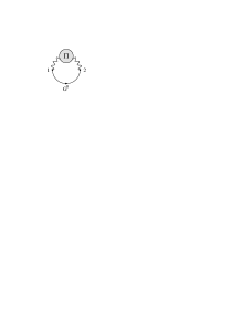
Figure 1: Feynman graph for the electron self energy $\Sigma(1,2)$

$\Pi$ is the self energy of the virtual photon and we have

$$i\Sigma^{<}(\textbf{p},t_{1},t_{2})=-e^{2}\gamma_{\mu}\left(\int\frac{d^{3}k}{(2\pi)^{3}}D_{\gamma}^{<\,\mu\nu}(\textbf{k},t_{1},t_{2})G^{<}_{0}(\textbf{p}-\textbf{k},t_{1},t_{2})\right)\gamma_{\nu}\text{,}$$ (12)

with $D_{\gamma}^{<\,\mu\nu}(\textbf{k},t_{1},t_{2})$ being the propagator of the dressed virtual photon with momentum k. Inserting this with the explicit form of the free electron propagator (9) into Eq. (11) yields

$$\partial_{\tau}N(\textbf{p},\tau)=2~{}\text{Re} \left[e^{2}\int_{t_{0}}^{\tau}d\bar{t}\int\frac{d^{3}k}{(2\pi)^{3}}(i)D_{\gamma}^{<\,\mu\nu}(\textbf{k},\tau,\bar{t})e^{iE_{\textbf{p}}(\tau-\bar{t})}e^{E_{\textbf{p}-\textbf{k}}(\tau-\bar{t})}\right.$$

$$~{}~{}~{}~{}\left.\times\frac{1}{2E_{\textbf{p}}}\frac{1}{2E_{\textbf{p}-\textbf{k}}}\text{\text{Tr}}\left\{(\not{p}+m)\gamma_{\mu}(\gamma_{0}E_{\textbf{p}-\textbf{k}}+\mbox{\boldmath$\gamma$}\cdot(\textbf{p}-\textbf{k})-m)\gamma_{\nu}\right\}\right]\text{,}$$ (13)

where evaluation of the trace leads to

$$\partial_{\tau}N(\textbf{p},\tau) =2~{}e^{2}~{}\int\frac{d^{3}k}{(2\pi)^{3}}\frac{1}{E_{\textbf{p}}}\frac{1}{E_{\textbf{p}-\textbf{k}}}\left[p_{\mu}(k-p)_{\nu}+p_{\nu}(k-p)_{\mu}-g_{\mu\nu}(p_{\mu}(k-p)^{\mu}+m^{2})\right]$$

$$~{}~{}~{}~{}\times\text{Re}\left[\int_{t_{0}}^{\tau}d\bar{t}iD_{\gamma}^{<\,\mu\nu}(\textbf{k},\tau,\bar{t})e^{i(E_{\textbf{p}}+E_{\textbf{k}-\textbf{p}})(\tau-\bar{t})}\right]\text{.}$$ (14)

Defining $p^{-}=k-p$ and $p^{+}=p$ as the four-momenta of the outgoing electron and positron, we rewrite Eq. (14) to

$$E_{+}E_{-}\frac{dR}{d^{3}p^{+}d^{3}p^{-}}(\tau)= \frac{2e^{2}}{(2\pi)^{6}}\left[p_{\mu}^{+}p_{\nu}^{-}+p_{\nu}^{+}p_{\mu}^{-}-g_{\mu\nu}(p^{+}p^{-}+m^{2})\right]$$

$$~{}~{}~{}~{}\times\text{Re}\left[\int_{t_{0}}^{\tau}d\bar{t}iD_{\gamma}^{<\,\mu\nu}(\textbf{k},\tau,\bar{t})e^{i(E_{+}+E_{-})(\tau-\bar{t})}\right]\text{,}$$ (15)

with $E_{-}=E_{\textbf{k}-\textbf{p}}$ and $E_{+}=E_{\textbf{p}}$. $R$ denotes the number of lepton pairs per unit four-volume, produced with the specified momentum configuration. We now show that Eq. (15) is indeed the generalization of the well known thermal production rate for lepton pairs McLerran and Toimela (1985); Weldon (1990); Gale and Kapusta (1991). Using the Fourier transform in relative time coordinates, defined by

$$D_{\gamma}^{<\,\mu\nu}(\textbf{k},\tau,\bar{t})=\int\frac{d\omega}{2\pi}D_{\gamma}^{<\,\mu\nu}(\textbf{k},\tau,\omega)e^{-i\omega(\tau-\bar{t})}\text{,}$$ (16)

and taking $t_{0}\rightarrow-\infty$, we have for the stationary case:

$$E_{+}E_{-}\frac{dR}{d^{3}p^{+}d^{3}p^{-}}= \frac{2e^{2}}{(2\pi)^{6}}\left[p_{\mu}^{+}p_{\nu}^{-}+p_{\nu}^{+}p_{\mu}^{-}-g_{\mu\nu}(p^{+}p^{-}+m^{2})\right]$$

$$~{}~{}~{}~{}\times\text{Re}\left[i\int\frac{d\omega}{2\pi}D_{\gamma}^{<\,\mu\nu}(\textbf{k},\omega)\int_{-\infty}^{\tau}d\bar{t}e^{i(E_{+}+E_{-}-\omega)(\tau-\bar{t})}\right]$$ (17)

$iD_{\gamma}^{<\,\mu\nu}(\textbf{k},\omega)$ is real and time independent in the stationary case. The real part of the last integral is simply $\pi\delta(E_{+}+E_{-}-\omega)$. With that and the virtual photon momentum $k^{\mu}=(E,\textbf{k})$, $E=E_{+}+E_{-}$, the rate becomes

$$E_{+}E_{-}\frac{dR}{d^{3}p^{+}d^{3}p^{-}} =-\frac{e^{2}}{(2\pi)^{6}}\left[p_{\mu}^{+}p_{\nu}^{-}+p_{\nu}^{+}p_{\mu}^{-}-g_{\mu\nu}(p^{+}p^{-}+m^{2})\right]D_{\gamma}^{<\,\mu\nu}(k)$$

$$=-\frac{e^{2}}{(2\pi)^{6}}\left[p_{\mu}^{+}p_{\nu}^{-}+p_{\nu}^{+}p_{\mu}^{-}-g_{\mu\nu}(p^{+}p^{-}+m^{2})\right]\frac{1}{M^{4}}\Pi_{\gamma}^{<\,\mu\nu}(k)$$

$$=-\frac{2e^{2}}{(2\pi)^{6}}\left[p_{\mu}^{+}p_{\nu}^{-}+p_{\nu}^{+}p_{\mu}^{-}-g_{\mu\nu}(p^{+}p^{-}+m^{2})\right]\frac{1}{M^{4}}\frac{1}{e^{\beta E}-1}\text{Im}\Pi_{\gamma}^{\text{ret}\,\mu\nu}(k)\text{,}$$ (18)

where we used Eq. (6) for $D_{\gamma}^{<\,\mu\nu}(k)$ in its stationary limit in the first step as well as $\Pi^{<}=2in_{\text{B}}\text{Im}\Pi^{\text{ret}}$, which follows from the Kubo-Martin-Schwinger (KMS) relation Kubo (1957); Martin and Schwinger (1959); Greiner and Leupold (1998), in the second step. Eq. (18) is the well known rate of dilepton production derived in e.g. Gale and Kapusta (1991).

We return to the nonequilibrium formula (15) and project on the virtual photon momentum using

$$\frac{dN}{d^{4}xd^{4}k}=\int\frac{dR}{d^{3}p^{+}d^{3}p^{-}}\delta^{4}(p^{+}+p^{-}-k)d^{3}p^{+}d^{3}p^{-}\text{.}$$

This leads to

$$\frac{dN}{d^{4}xd^{4}k}(\tau,\textbf{k},E)= \frac{2e^{2}}{(2\pi)^{6}}\int\frac{d^{3}p^{+}}{E_{+}}\int\frac{d^{3}p^{-}}{E_{-}}\delta^{4}(p^{+}+p^{-}-k)\left[p_{\mu}^{+}p_{\nu}^{-}+p_{\nu}^{+}p_{\mu}^{-}-g_{\mu\nu}(p^{+}p^{-}+m^{2})\right]$$

$$~{}~{}~{}~{}\times\text{Re}\left[\int_{t_{0}}^{\tau}d\bar{t}iD_{\gamma}^{<\,\mu\nu}(\textbf{k},\tau,\bar{t})e^{iE(\tau-\bar{t})}\right]\text{}$$ (19)

for the production rate of dilepton pairs of momentum $k=(E=E_{+}+E_{-},\textbf{k})$. In the following numerical study we will consider the mode $\textbf{k}=0$ exclusively, i.e., the virtual photon resting with respect to the medium. For this case, and taking the electron mass $m$ to zero, Eq. (19) can be simplified to

$$\frac{dN}{d^{4}xd^{4}k}(\tau,\textbf{k}=0,E)= \frac{2e^{2}}{(2\pi)^{6}}\frac{2}{3}\pi(k_{\mu}k_{\nu}-k^{2}g_{\mu\nu})\text{Re}\left[\int_{t_{0}}^{\tau}d\bar{t}iD_{\gamma}^{<\,\mu\nu}(\textbf{k}=0,\tau,\bar{t})e^{iE(\tau-\bar{t})}\right]\text{.}$$ (20)

This expression is easily understood. The dynamic information is inherent in the memory integral on the right hand side that runs over all virtual photon occupation numbers, Fourier transformed at energy $E$ from the initial time to the present. Hence this memory integral determines the full nonequilibrium dilepton production rate at time $\tau$.

II.3 The in-medium virtual photon self energy $\Pi$

The dilepton production rate (20) involves the virtual photon occupation number, expressed by the propagator $D_{\gamma}^{<}$. We introduce the dynamic medium dependence by dressing this virtual photon propagator with the medium dependent $\rho$- or $\omega$-meson. This dressing enters via the photon self energy $\Pi^{<}$ through the fluctuation dissipation relation (cf. (6)) for $D_{\gamma}^{<\,\mu\nu}$:

$$D_{\gamma}^{<\,\mu\nu} =D_{\gamma}^{\text{ret}\,\mu\alpha}\odot\Pi^{<}_{\alpha\beta}\odot D_{\gamma}^{\text{adv}\,\beta\nu}\text{,}$$ (21)

where $\odot$ implies the integration over intermediate space-time coordinates. In the medium the vector mesons and virtual photons have two possible polarizations relative to their momentum in the medium. This leads to two different self energies $\Pi_{\text{T}}$ (transverse) and $\Pi_{\text{L}}$ (longitudinal). Introduction of the projectors $P_{\text{L}}$ and $P_{\text{T}}$ allows us to split the propagators and the self energy into a 3-longitudinal and a 3-transversal part, relatively to the particle’s momentum Weldon (1990):

$$D_{\gamma}^{\text{ret}\,\mu\alpha}=-\frac{P_{\text{T}}^{\mu\alpha}}{k^{2}-\Pi_{\text{T}}^{\text{ret}}}-\frac{P_{\text{L}}^{\mu\alpha}}{k^{2}-\Pi_{\text{L}}^{\text{ret}}}\text{~{};~{}~{}}D_{\gamma}^{\text{adv}\,\beta\nu}=-\frac{P_{\text{T}}^{\beta\nu}}{k^{2}-\Pi_{\text{T}}^{\text{ret}*}}-\frac{P_{\text{L}}^{\beta\nu}}{k^{2}-\Pi_{\text{L}}^{\text{ret}*}}$$ (22)

and

$$\Pi^{<}_{\alpha\beta}=-P_{\text{T}\,\alpha\beta}\Pi_{\text{T}}^{<}-P_{\text{L}\,\alpha\beta}\Pi_{\text{L}}^{<}\text{.}$$ (23)

The projectors fulfill the usual projector properties $P_{(\text{T}/\text{L})}^{2}=P_{(\text{T}/\text{L})}$ and $P_{\text{T}}P_{\text{L}}=P_{\text{L}}P_{\text{T}}=0$. With that, Eq. (21) becomes

$$D_{\gamma}^{<\,\mu\nu} =D_{\gamma}^{\text{ret}\,\mu\alpha}\odot(-P_{\text{T}\,\alpha\beta}\Pi_{\text{T}}^{<}-P_{\text{L}\,\alpha\beta}\Pi_{\text{L}}^{<})\odot D_{\gamma}^{\text{adv}\,\beta\nu}$$

$$=-D_{\gamma,\text{T}}^{<}P_{\text{T}}^{\mu\nu}-D_{\gamma,\text{L}}^{<}P_{\text{L}}^{\mu\nu}\text{,}$$ (24)

with

$$D_{\gamma,\text{T/L}}^{<}=\frac{1}{k^{2}-\Pi_{\text{T/L}}^{\text{ret}}}\odot\Pi_{\text{T/L}}^{<}\odot\frac{1}{k^{2}-\Pi_{\text{T/L}}^{\text{ret}*}}\text{.}$$ (25)

In the case $\textbf{k}=0$, considered later, the longitudinal and transverse parts become identical and it follows

$$D_{\gamma}^{<\,\mu\nu} =-D^{<}_{\gamma,\text{T}}P_{\text{T}}^{\mu\nu}-D_{\gamma,\text{T}}^{<}P_{\text{L}}^{\mu\nu}=-D_{\gamma,\text{T}}^{<}(P_{\text{T}}^{\mu\nu}+P_{\text{L}}^{\mu\nu})=-D_{\gamma,\text{T}}^{<}\left(g^{\mu\nu}-\frac{k^{\mu}k^{\nu}}{k^{2}}\right)\text{.}$$

In this case the production rate depends only on the transverse part of the virtual photon propagator. The appearing factor of $3$ accounts for the two transverse and one longitudinal directions:

$$\frac{dN}{d^{4}xd^{4}k}(\tau,\textbf{k}=0,E)= \frac{2}{3}\frac{e^{2}}{(2\pi)^{5}}(3E^{2})\text{Re}\left[\int_{t_{0}}^{\tau}d\bar{t}iD_{\gamma,\text{T}}^{<}(\textbf{k}=0,\tau,\bar{t})e^{iE(\tau-\bar{t})}\right]$$ (26)

For dilepton production $\Pi^{\text{ret}}\propto e^{2}$ and $E$ is the invariant mass of the virtual photon. For the cases, we are interested in, it holds $|\Pi^{\text{ret}}|\ll E$ and we can approximate

$$D_{\gamma,\text{T}}^{<}=D_{\gamma,0}^{\text{ret}}\odot\Pi_{\text{T}}^{<}\odot D_{\gamma,0}^{\text{adv}}\text{.}$$ (27)

For $\textbf{k}\rightarrow 0$

$$D_{\gamma,0}^{\text{ret}}(\textbf{k}\rightarrow 0,t)=-\theta(t)t=D_{\gamma,0}^{\text{adv}}(\textbf{k}\rightarrow 0,-t)$$ (28)

and we may calculate the virtual photon propagator using the transport equation

$$iD^{<}_{\gamma,\text{T}}(\textbf{k}=0,\tau,\bar{t}) =\int_{t_{0}}^{\tau}dt_{1}\int_{t_{0}}^{\bar{t}}dt_{2}~{}(\tau-t_{1})\left(i\Pi_{\text{T}}^{<}(\textbf{k}=0,t_{1},t_{2})\right)(\bar{t}-t_{2})\text{.}$$ (29)

The appearing undamped photon propagators lead to diverging contributions from early times, i.e., for low frequencies. In the later numerical calculation these contributions turn out to be at least of the order $10^{5}$ larger than the actual (higher frequency) structure. Due to the naturally limited numerical accuracy, the higher frequency structure would get lost among these early time contributions. In order to cure this numerical problem, we introduce an additional cutoff $\Lambda$ for the free photon propagators, i.e., we perform the replacement:

$$D_{\gamma,0}^{\text{ret}}(\tau-t_{1})=(\tau-t_{1})\rightarrow(\tau-t_{1})e^{-\Lambda(\tau-t_{1})}$$ (30)

and analogously for $D_{\gamma,0}^{\text{adv}}(t_{2}-\bar{t})$. In the performed calculations we employ $\Lambda\approx 0.3$ GeV. The exponential factors lead to a reduction of the rate, which we will overcome by renormalizing the final result by multiplication with $\frac{(\omega^{2}+\Lambda^{2})^{2}}{\omega^{4}}\text{,}$ a factor we get from Fourier transforming the convolution (29), assuming equilibrium. This will not affect the time scales we are interested in, and comparison of the dynamically computed rate for the stationary case (constant self energy) with the analytic thermal rate shows perfect agreement.

Vector meson dominance (VMD) Sakurai (1960, 1969) allows for the calculation of $\Pi_{\text{T}}^{<}$, using the identity between the electromagnetic current and the canonical interpolating fields of the vector mesons Kroll et al. (1967):

$$J_{\mu}=-\frac{e}{g_{\rho}}m_{\rho}^{2}\rho_{\mu}-\ldots\text{,}$$ (31)

which leads to

$$\Pi^{<}_{\alpha\beta}=\frac{e^{2}}{g_{\rho}^{2}}m_{\rho}^{4}D_{\rho\,\alpha\beta}^{<}\text{}$$ (32)

for the self energy. When treating the $\omega$-meson, we use the corresponding self energy and propagator. We again apply the generalized fluctuation dissipation relation (6) to calculate

$$D_{\rho,\text{T}}^{<}=D_{\rho,\text{T}}^{\text{ret}}\odot\Sigma^{<}_{\rho,\text{T}}\odot D_{\rho,\text{T}}^{\text{adv}}\text{,}$$ (33)

with the $\rho$-meson self energy $\Sigma^{<}_{\rho,\text{T}}$. The transverse parts of the retarded and advanced propagators $D_{\rho,\text{T}}^{\text{ret}}(\textbf{k},t_{1},t_{2})=D_{\rho,\text{T}}^{\text{adv}}(\textbf{k},t_{2},t_{1})$ of the vector meson in a spatially homogeneous and isotropic medium follow the equation of motion

$$\left(-\partial_{t_{1}}^{2}-m_{\rho}^{2}-\textbf{k}^{2}\right)D_{\rho,\text{T}}^{\text{ret}}(\textbf{k},t_{1},t_{2})-\int_{t_{2}}^{t_{1}}d\bar{t}\Sigma^{\text{ret}}_{\rho,\text{T}}(\textbf{k},t_{1},\bar{t})D_{\rho,\text{T}}^{\text{ret}}(\textbf{k},\bar{t},t_{2})=\delta(t_{1}-t_{2})\text{.}$$ (34)

In the following we will omit the index T for convenience.

The dynamic medium evolution is now introduced by hand via a specified time dependent retarded meson self energy $\Sigma^{\text{ret}}(\tau,\omega)$ with system time $\tau$ (see Section III.1). From that the self energy $\Sigma^{<}$, needed for solving Eq. (33), follows by introduction of an assumed background temperature of the fireball. The fireball, constituting the medium, generates the time dependent self energy $\Sigma^{\text{ret}}$ and, assuming a quasi thermalized system, the $\rho$-meson current-current correlator $\Sigma^{<}$ is given via

$$\Sigma^{<}(\tau,\omega,\textbf{k})=2in_{\text{B}}(T(\tau))\text{Im}\Sigma^{\text{ret}}(\tau,\omega,\textbf{k})\text{,}$$ (35)

which follows from the KMS relation

$$\Sigma^{<}(\omega,\textbf{k})=\mp e^{-\beta\omega}\Sigma^{>}(\omega,\textbf{k})\text{,}$$ (36)

being valid for thermal systems Kubo (1957); Martin and Schwinger (1959); Greiner and Leupold (1998). $n_{\text{B}}$ is the Bose-distribution. The assumption of a quasi thermalized background medium is of course rather strong, but necessary in order to proceed: In principle, for a full nonequilibrium situation the self energies $\Sigma^{<}$ and $\Sigma^{>}$ for the $\rho$-meson have to be obtained self-consistently via e.g. coupling to resonance-hole pairs Peters et al. (1998), being out of equilibrium themselves. (For a realization of true nonequilibrium dynamics of a homogeneous system within a $\Phi^{4}$-theory see Juchem et al. (2004a) and within a coupled fermion-meson system Berges et al. (2003).) For an expanding and inhomogeneous reaction geometry this is still not possible today. In any case, explicit calculation of $\Sigma^{<}$ in the two-time representation will cause even stronger memory effects. Additionally, in order to simulate a realistic situation by application of a fireball model, a temperature needs to be defined and hence local equilibrium has to be assumed.

The framework, we have established, allows us to calculate the dynamic evolution of vector mesons’ spectral properties, occupation, and the nonequilibrium dilepton production rate, given an evolving medium with assumed time dependent quasi-thermal properties. At this point it is also worthwhile to point out that working in the two-time representation has great advantages over the mixed representation, in which all quantities are expressed by their Wigner transforms. The problem in this case is that the Wigner transforms of the many appearing convolutions are nontrivial. They can be expressed by a gradient expansion to infinite order Henning (1995). Explicit calculations are usually carried out within a first order gradient approximation, which is not applicable in our case because the system is not evolving slowly with respect to the relevant time scales (see Sections III.3 and III.6 for details on the time scales involved). All memory is lost by application of this approximation, because when using the mixed representation, full Fourier transformations from relative time to its conjugate frequency are involved, which imply treating contributions from the future and from the past on equal grounds. This violates causality in a quickly evolving system. Hence, calculations within the two-time representation allow for the most exact investigation of the evolving system under consideration.

III Nonequilibrium dilepton production from an evolving medium

III.1 Vector meson self energies

We are now able to calculate the evolution of the spectral properties of vector mesons in a changing medium as well as the corresponding dilepton production rates. We will treat mass shifts described by Brown-Rho scaling Brown and Rho (1991), broadening, as caused by pion scattering, and scattering of the mesons with nucleons, leading to further broadening and excitation of resonances Herrmann et al. (1992); Chanfray and Schuck (1992); Rapp et al. (1996); Friman and Pirner (1997); Klingl et al. (1997); Peters et al. (1998); Post et al. (2004). The medium effects are introduced via a specific time evolving self energy for the vector mesons. The main purpose of this work is to investigate medium modifications dynamically for the first time, and compare the results to those obtained from instantaneous, Markovian calculations.

In the following we first employ simplified self energies for possible broadening such as

$$\text{Im}\Sigma^{\text{ret}}(\tau,\omega)=-\omega\Gamma(\tau)\text{,}$$ (37)

with a k- and $\omega$-independent width $\Gamma$, which, in the static case, leads to a Breit-Wigner distribution of the spectral function

$$A(\omega,\textbf{k}) =-\frac{1}{\pi}\text{Im}D_{\rho}^{\text{ret}}(\omega,\textbf{k})=\frac{1}{\pi}\frac{\omega\Gamma}{(\omega^{2}-\textbf{k}^{2}-m^{2})^{2}+(\omega\Gamma)^{2}}\text{.}$$ (38)

The self energy (37) is given in a mixed time-frequency representation. The time dependence is being accounted for by introduction of the system time $\tau$, for which we will discuss two possible choices below. $\omega$ stems from the Fourier transformation in relative time $(t_{1}-t_{2})$.

Modifications of the mass are introduced directly as via a local term in the self energy. From this sort of self energy several numerical issues emerge. In Eq. (34) the self energy enters in time representation

$$\Sigma^{\text{ret}}(t_{1},t_{2})=(\Sigma^{>}(t_{1},t_{2})-\Sigma^{<}(t_{1},t_{2}))\theta(t_{1}-t_{2})\text{,}$$ (39)

Its Fourier transform in relative time $(t_{1}-t_{2})$, $\Sigma^{ret}(\tau,\omega)$, is given by a convolution of the $\theta$-function’s Fourier transform and $(\Sigma^{>}-\Sigma^{<})(\tau,\omega)$:

$$\Sigma^{\text{ret}}(\tau,\omega) =i\int\frac{d\bar{\omega}}{2\pi}\frac{1}{\omega-\bar{\omega}+i\epsilon}(\Sigma^{>}-\Sigma^{<})(\tau,\bar{\omega})$$

$$=i\mathcal{P}\int\frac{d\bar{\omega}}{2\pi}\frac{1}{\omega-\bar{\omega}}(\Sigma^{>}-\Sigma^{<})(\tau,\bar{\omega})+\frac{1}{2}(\Sigma^{>}-\Sigma^{<})(\tau,\omega)\text{,}$$ (40)

where we used the standard relation

$$\frac{1}{\omega-\bar{\omega}+i\epsilon}=\mathcal{P}\frac{1}{\omega-\bar{\omega}}-i\pi\delta(\omega-\bar{\omega})\text{.}$$ (41)

With $(\Sigma^{>}-\Sigma^{<})(\tau,\omega)=-2i\omega\Gamma(\tau)$, one has

$$\Sigma^{\text{ret}}(\tau,\omega) =2\mathcal{P}\int_{-c}^{+c}\frac{d\bar{\omega}}{2\pi}\frac{\bar{\omega}}{\omega-\bar{\omega}}\Gamma(\tau)-i\omega\Gamma(\tau)\text{,}$$

which has the imaginary part (37). In addition we also get an ”unwanted” dispersive real part that causes an (infinite) mass shift. The introduced cutoff $c$ cures that infinity and we can renormalize the mass by the replacement

$$m\rightarrow\sqrt{m^{2}-\text{Re}\Sigma^{ret}(\omega,\tau)}\text{,}$$

with

$$\text{Re}\Sigma^{\text{ret}}(\tau,\omega) =\text{Re}\left[2\Gamma(\tau)\mathcal{P}\int_{-c}^{+c}\frac{d\bar{\omega}}{2\pi}\frac{\bar{\omega}}{\omega-\bar{\omega}}\right]$$

$$=-\frac{2}{\pi}\Gamma(\tau)c\left({}_{2}F_{1}\left(-\frac{1}{2},1,\frac{1}{2},\frac{\omega^{2}}{c^{2}}\right)\right)$$

$$\approx-\frac{2}{\pi}\Gamma(\tau)c\left(1-\frac{\omega^{2}}{c^{2}}-\frac{\omega^{4}}{3c^{4}}\right)\text{,}$$ (42)

with the hypergeometric function ${}_{2}F_{1}$, Taylor expanded to second order in the last line. To make the renormalization $\omega$-independent, we replace $\omega$ by the physical pole mass $m$, causing only minimal inaccuracies far from the peak position.

Another potential problem is the behavior of the self energy $\Sigma^{<}(\tau,\omega)$ for negative frequencies. As already described, for a thermalized system, it is given by $\Sigma^{<}(\tau,\omega)=2in_{\text{B}}(T(\tau),\omega)\text{Im}\Sigma^{\text{ret}}(\tau,\omega)$. For negative frequencies the propagator $D^{<}(\tau,\omega)$ contains a factor of $(1+n(\omega))$ since there holds the symmetry relation $D^{<}(\tau,-\omega)=D^{>}(\tau,\omega)$ for the scalar boson case and $D^{>}(\tau,\omega)=2i(1+n_{\text{B}})A(\tau,\omega)$ in equilibrium. The first term in parentheses leads to divergent vacuum contributions, which are uninteresting for the investigation of the positive frequency behavior and cause numerical problems. To see this, we first give the limits of the expression $\Sigma^{<}(\tau,\omega)$ in frequency representation:

$$i\Sigma^{<}(\tau,\omega)=\left\{\begin{array}[]{rl}\propto e^{-\omega/T(\tau)}&\text{for }\omega\gg 0\\ 2T(\tau)\Gamma(\tau)&\text{for }\omega=0\\ -2\omega\Gamma(\tau)&\text{for }\omega\ll 0\end{array}\right.$$ (46)

The Fourier transform thus becomes a $\delta^{\prime}$-distribution for the negative frequency part. In order to cure this problem we first split the self energy into positive and negative frequency parts

$$i\Sigma^{<}(\tau,\omega) =\underbrace{\frac{2|\omega|\Gamma(\tau)}{e^{|\omega|/T(\tau)}-1}}_{=:i\Sigma^{<,\text{eff}}(\tau,\omega)}-2\omega\Gamma(\tau)\theta(-\omega)\text{,}$$ (47)

and neglect the negative frequency part, violating the mentioned symmetry relation for $D^{<}$ and $D^{>}$ (also for $\Sigma^{<}$ and $\Sigma^{>}$). This violation however only means an omittance of the vacuum contributions for negative frequencies and does not cause changes for positive frequencies. The same approach may be taken with other types of self energies having the same symmetry property under the exchange $\omega\leftrightarrow-\omega$.

Coupling of resonances to the $\rho-N$-channel has been treated by Friman and Pirner (1997); Peters et al. (1998); Post et al. (2004). For the $\textbf{k}=0$ mode, the full self energy for coupling to $J^{P}=\frac{3}{2}^{-}$ -resonances is given by Post et al. (2004) (also see Henning and Umezawa (1994), who treated coupling of pions to resonance hole excitations)

$$\text{Im}\Sigma(\tau,\omega,\textbf{k}=0)=-\frac{\rho(\tau)}{3}\left(\frac{f_{RN\rho}}{m_{\rho}}\right)^{2}g_{I}\frac{\omega^{3}\bar{E}\Gamma_{R}(\tau)}{(\omega^{2}-\bar{E}^{2}-\frac{\Gamma_{R}(\tau)^{2}}{4})^{2}+(\Gamma_{R}(\tau)\omega)^{2}}-\omega\Gamma(\tau)\text{.}$$ (48)

$\bar{E}=\sqrt{m_{R}^{2}+\textbf{k}^{2}}-m_{N}$ is the energy necessary for the meson to scatter from a nucleon at rest, with $m_{R}$ and $m_{N}$ the masses of the resonance and the nucleon respectively. $\Gamma_{R}$ is the width of the resonance and $g_{I}$ is the isospin factor ($2$ for isospin $\frac{1}{2}$ and $\frac{4}{3}$ for isospin $\frac{3}{2}$ resonances). $\rho(\tau)$ is the time dependent density of the system and appears due to application of the $\rho$-$\cal T$-approximation, where $\cal T$ stands for the forward scattering amplitude. The important part for our purpose is the structure of the denominator, which represents a characteristic pole structure. We will replace $\omega^{2}$ in the numerator by a constant factor since it causes divergence of $\text{Re}\Sigma^{\text{ret}}$, only cured by application of subtracted dispersion relations corresponding to counterterms. The cutoff $c$ also prevents divergences but leaving in the factor of $\omega^{2}$ causes inaccurate numerical results. We show the spectral function for the case of the $N(1520)$ resonance, where $f_{RN\rho}\approx 7.0$ Peters et al. (1998) and the width of the resonance is $\Gamma_{R}=120$ GeV, in Fig. 2 for different densities at $\textbf{k}=0$.

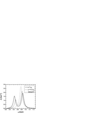
Figure 2: Spectral function of the $\rho$-meson coupled to an N(1520)-hole pair for different densities. $\bar{E}=582$ MeV,$\Gamma_{R}=120$ MeV

We now discuss the system time $\tau$. Defining $\tau=\frac{t_{1}+t_{2}}{2}$, as first done in Kadanoff and Baym (1962), seems to be a sensible choice, but when investigating the spectral function, one is dealing with retarded quantities and we do not want them to collect information from the future, i.e., we want to retain causality. This is why we choose $\tau=t_{1}$ instead of the symmetric form $\tau=\frac{t_{1}+t_{2}}{2}$, because in this case at a certain time $\tau$ information of $\Sigma^{\text{ret}}$ that is located in the future of $\tau$ enters the spectral function. This cannot happen with $\tau=t_{1}$ as demonstrated in Appendix A.

For the self energy $\Sigma^{<}(\tau,\omega)$ one should stick to the symmetric choice in order to fulfill the symmetry relation $\Sigma^{<}(t_{1},t_{2})=\Sigma^{>}(t_{2},t_{1})$. However, doing this reduces accuracy in the numerical calculation, due to additional necessary Fourier transformations. Comparison of calculations using either $\Sigma^{<}(t_{1},\omega)$ or $\Sigma^{<}(\frac{t_{1}+t_{2}}{2},\omega)$ reveals minor differences in the rate when changing the temperature with system time $t_{1}$ or $\frac{t_{1}+t_{2}}{2}$ respectively, but on average, and hence in the final yield, the differences cancel, as could be expected.

III.2 Contributions to the rate in time representation

Before we calculate nonequilibrium rates and yields, we investigate how the present rate is created over time, i.e., we focus on which contributions to Eq. (26) come from which times in the past. Figs. 3 and 4 show the integrand for fixed energy $\omega=750$ MeV and fixed time $\tau$ for relative times $\tau-t$. The first case shown (left of Fig. 3) is an equilibrium scenario with free $\rho$-mesons embedded in an environment at constant temperature. One can see that the main contribution comes from the very near past, but that there are also contributions from early times as well as large oscillations leading to alternating positive and negative contributions. The second case (right of Fig. 3) represents $\rho$-mesons, embedded in a constant heat bath, broadened and coupled to the N(1520) resonance at the time where the coupling and broadening was completely turned off again 10 fm/c ago in a way that will be discussed in Section III.3 (over a time of $\Delta\tau=7.18$ fm/c, cf. Fig. 6 - We use this duration because it results as the lifetime of the hadronic phase of the fireball from calculations described in Section III.6 and will hence be used in calculations of the dilepton yields). The integrand shows richer structures than in the equilibrium case, caused by the changing self energy in the past, which is quite remarkable: It shows that after having exposed the $\rho$-mesons to vacuum conditions for 10 fm/c, a memory of the situation in the more distant past is remaining. The third case (Fig. 4) again represents free $\rho$-mesons but with the production in the heat bath, caused by $\Sigma^{<}_{\rho}$, turned off $10$ fm/c in the past. Comparison of the overall amplitude to that in Fig. 3 (left) shows that the rate at time $\tau$, resulting from the integral over the function shown in Fig. 4 (see Eq. (26)), will be very small compared to the rate before production was turned off, which is clear since the $\rho$-meson has a decay constant of 1.3 fm/c with that the rate is exponentially suppressed after production is turned off. The shape of the contribution is very interesting: Between the point where production was turned off and the present the integrand has a decaying (and oscillating) shape and contributions from the more distant past also remain. However, the largest values, contributing to the present rate, are situated close to the time, at which production was turned off. This is intuitively clear. The dileptons produced at the present time $\tau$ most dominantly originate from decaying $\rho$-mesons, produced slightly before the time when production was turned off. Thereby the strong memory to that past time is visible in the integrand.

Figure 3: Contributions to the rate for a fixed frequency at given time $\tau$ from times $(\tau-t)$ in the past for the case of free $\rho$-mesons at constant temperature (left) and the case where the coupling to the N(1520) was turned off 10 fm/c before the present time (widths were also changed as indicated in the figure (see text) - index 1 refers to initial, 2 to final quantities) (right).

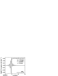
Figure 4: Contributions to the rate for a fixed frequency at given time $\tau$ from times $(\tau-t)$ in the past. The production has been turned off 10 fm/c before the present time $\tau$.

A full interpretation of the various structures shown is difficult and it becomes clear that only the completely integrated yield represents a physical quantity. There is a dependence on the parameter $\Lambda$ (cf. Eq. (30) and related discussion) such that contributions from times further in the past are reduced using larger cutoffs $\Lambda$. On the other hand the accuracy of the numerics is strongly increased by employing larger cutoffs (when setting $\Lambda$ to zero all the principal information is destroyed by diverging contributions, several orders of magnitude larger than the actual structure responsible for the creation of the rate). The early time contributions translate to diverging contributions for the smallest frequencies after Fourier transformation. The comparison of the rate from a free $\rho$-meson at constant temperature (i.e., the equilibrium case) calculated dynamically and the one calculated using the equilibrium formula

$$\frac{dN}{d^{4}xd^{4}k}(\omega)=\frac{2e^{4}}{(2\pi)^{5}}\frac{m_{\rho}^{4}}{g_{\rho}^{2}}\frac{1}{\omega^{2}}n_{\text{B}}(\omega)\pi A(\omega)\text{,}$$ (49)

shows that the dynamically calculated rates, being integrals over strongly oscillating functions, as shown in Figs. 3 and 4, are reproduced very well by the numerics as nicely seen in Fig. 5. Here one also notices the large contributions at low frequencies, which cause the mentioned numerical uncertainties and therefore have to be reduced by introduction of the mentioned cutoff $\Lambda$. These contributions are being many orders of magnitude larger than those for frequencies at the upper end of the regarded range.

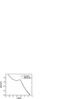
Figure 5: Comparison of the dynamically calculated rate (solid) to the one calculated from Eq. (49), the Markovian rate (dashed), shows very good agreement.

III.3 Time scales of adaption for the spectral function, occupation number and dilepton rate

In order to quantify the times that the mesons’ spectral properties need to adjust to the evolving medium, we regard the cases of broadening and mass shifts and introduce a time dependent self energy that represents linear changes (see Fig. 6) in width or mass.

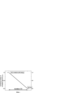
Figure 6: Linear switching off of in-medium effects over a certain duration $\Delta\tau$

We do not perform sudden changes using step functions in time because that would cause strong, hard to control oscillations in the Fourier transforms. Apart from the linear function, totally smooth functions like a hyperbolic tangent have been tested for the representation of the time evolution. It was found that the two kinks in the linear function do not cause additional problems when Fourier transforming. Hence, we chose this representation for the time evolution because it allows for the precise definition of the duration of the change, and by that of the time scale, which is not possible for absolutely smooth functions.

The spectral function is given by the imaginary part of the Fourier transform in relative time coordinates of the retarded meson-propagator

$$D_{\rho}^{\text{ret}}(t_{1},t_{2})\rightarrow D_{\rho}^{\text{ret}}(\tau,t_{1}-t_{2})\rightarrow-\frac{1}{\pi}\text{Im}D_{\rho}^{\text{ret}}(\tau,\omega)=A(\tau,\omega)\text{,}$$ (50)

where the system time $\tau$ is chosen to be $t_{1}$ for reasons discussed at the end of Section III.1 and in Appendix A. Taking $\tau$ to be $\frac{t_{1}+t_{2}}{2}$ leads to an about two times faster adjustment of the spectral function, which is caused by the fact that it is now able to gain information on the medium symmetrically from the past and the future, which is unphysical.

The spectral functions’s retardation with respect to medium changes is found by comparing the dynamically calculated spectral function at the time $\tau_{\text{off}}$ when the medium effects are fully turned off and the one calculated at the same time, assuming an instantaneous adaption. This spectral function is given directly by

$$A_{\text{Markov}}(\tau,\omega) =-\frac{1}{\pi}\text{Im}D_{\rho\,\text{Markov}}^{\text{ret}}(\tau,\omega)=\frac{1}{\pi}\frac{-\text{Im}\Sigma_{\rho}^{\text{ret}}(\tau,\omega)}{(\omega^{2}-m_{\rho}^{2}-\text{Re}\Sigma_{\rho}^{\text{ret}}(\tau,\omega))^{2}+(\text{Im}\Sigma_{\rho}^{\text{ret}}(\tau,\omega))^{2}}$$ (51)

The difference can be made explicit by calculating the difference in the moment $\int_{0}^{\infty}A(\tau_{\text{off}},\omega)^{2}\omega^{2}d\omega$ of the two spectral functions or the difference in the peak position or height for mass shifts or broadening respectively. As an illustration of the procedure the spectral functions, which are compared, are shown for a particular example of in-medium broadening in Fig. 7 (full and dotted line). All methods lead to similar results. We find an exponentially decreasing difference with increasing duration of the change $\Delta\tau$ (see Fig. 6). From this exponential drop we extract a time constant $\bar{\tau}$, that for the case of broadening (and constant masses) is shown in Table 1 for different scenarios. Table 2 shows time scales for the adjustment of the spectral function to changes in the meson’s mass, extracted from the peak position. Due to oscillations in the changing spectral function (see below) an exact extraction of a time scale is more complicated in this case, but the numbers still give a magnitude for the retardation.

In the case of the $\rho$-meson ($\Gamma_{\text{vac}}\approx\Gamma_{2}=150$ MeV) we find a time scale of about 3 fm/c. That means that the behavior of the $\rho$ mesons becomes adiabatic only for medium changes that are slow compared to the time of 3 fm/c, i.e., the spectral properties follow the changes in the medium nearly instantaneously only if the evolution is very slow as compared to the derived time scale. For real heavy ion reactions this means that the spectral properties of vector mesons will retain a certain memory of the past, and even if they decay outside the medium, they still carry a certain amount of information on the medium in that they were produced. This can become important, especially for $\omega$-mesons, having a vacuum width of $8.49$ MeV Eidelman et al. (2004). Nevertheless, due to oscillations in the spectral function and rate and occurring interferences when calculating the dilepton yield (see below), this strong retardation may be put into perspective because the only physically meaningful influence of this retardation is that on the resulting yield (see Section III.6). We find the relation

$$\bar{\tau}\propto\frac{c}{\Gamma_{2}}\text{, with $c$ between $2$ and $3.5$.}$$ (52)

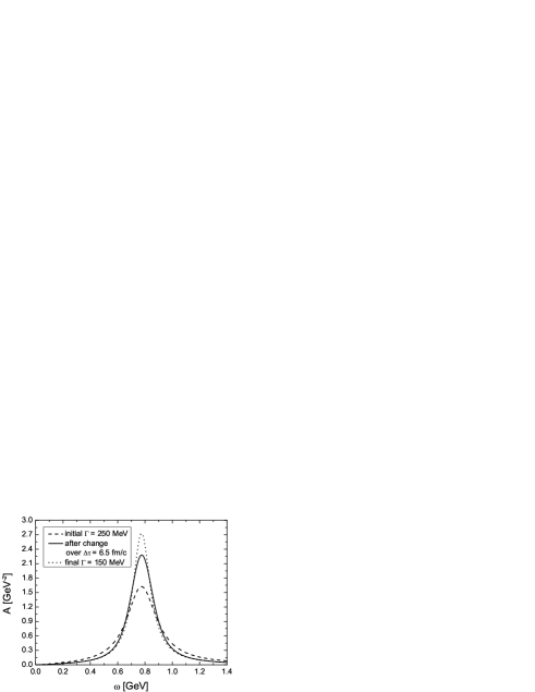
Figure 7: The two compared spectral functions right after the full change of the self energy is reached: dynamic (full) and Markovian (equals the final spectral function with $\Gamma=150$ MeV) (dotted) calculation. The initial spectral function (dashed) is also shown.

$\Gamma_{2}[\text{MeV}]$	$\bar{\tau}$ [fm/c] for	$\bar{\tau}$ [fm/c] for	$\bar{\tau}$ [fm/c] for	$\bar{\tau}$ [fm/c] for	$\bar{\tau}$ [fm/c] for	$\bar{\tau}$ [fm/c] for
	$m=570\text{ MeV}$	$m=570\text{ MeV}$	$m=570\text{ MeV}$	$m=770\text{ MeV}$	$m=770\text{ MeV}$	$m=770\text{ MeV}$
	$\Gamma_{1}=200\text{ MeV}$	$\Gamma_{1}=300\text{ MeV}$	$\Gamma_{1}=400\text{ MeV}$	$\Gamma_{1}=200\text{ MeV}$	$\Gamma_{1}=300\text{ MeV}$	$\Gamma_{1}=400\text{ MeV}$
150	2.4	3	3	2.8	3.6	3.2
90	5	5.2	6	4.8	5.4	6.2
70	6.4	7.2	8.2	6.4	7.2	8.2
50	9.4	10.8	12.8	8.8	10.4	12.2
30	16.4	20.4	24.8	13.6	17.4	21.2

Table 1: Values of $\bar{\tau}$ for different masses, initial widths $\Gamma_{1}$ and final widths $\Gamma_{2}$.

$\Delta m[\text{MeV}]$	$\bar{\tau}$ [fm/c] for	$\bar{\tau}$ [fm/c] for	$\bar{\tau}$ [fm/c] for
	$\Gamma=100\text{ MeV}$	$\Gamma=150\text{ MeV}$	$\Gamma=300\text{ MeV}$
100	4.33	3.12	2.15
300	5.5	3.82	2.14
400	6.5	3.97	2.16

Table 2: Values of $\bar{\tau}$ for different widths and mass shifts $\Delta m$ to masses below the final vacuum mass $m_{2}=770$ MeV.

$c$ depends on the other quantities $m$ and $\Gamma_{1}$ such that for a larger change in width, the spectral function takes longer to adjust to it. The reason for the time scale to be (at least) $2/\Gamma$ is that the spectral function is given by the imaginary part of the retarded propagator, which, representing a probability amplitude, is proportional to $e^{-\frac{1}{2}\Gamma t}$. Its square, an actual probability, is proportional to $e^{-\Gamma t}$, giving the appropriate decay rate.

This result can also be easily retrieved analytically when we assume a Breit-Wigner type self energy with constant width as well as a constant mass and solve the equation of motion that follows directly from Eq. (34)

$$\left(-\partial_{t_{1}}^{2}-m_{\rho}^{2}\right)D_{\rho,\text{T}}^{\text{ret}}(t_{1},t_{2})-\partial_{t_{1}}D_{\rho,\text{T}}^{\text{ret}}(t_{1},t_{2})\Gamma=\delta(t_{1}-t_{2})$$ (53)

by

$$D_{\rho,\text{T}}^{\text{ret}}(t_{1},t_{2})=-2\Theta(t_{1}-t_{2})\frac{1}{\sqrt{4m^{2}-\Gamma^{2}}}e^{-\frac{1}{2}\Gamma(t_{1}-t_{2})}\text{sin}(\frac{1}{2}\sqrt{4m^{2}-\Gamma^{2}}(t_{1}-t_{2}))$$ (54)

and we find the decay width to be $\Gamma/2$. The numerical solution shows the same behavior, but here we can go further and apply changes e.g. to the mass and see how the propagator behaves in time. In Fig. 8 we show the numerical solution for the retarded propagator in time representation $D_{\rho,T}^{\text{ret}}(\tau,t)$ at different fixed times $\tau$, for a constant width $\Gamma=150$ MeV and a mass, changed from $400$ to 770 MeV ($\tau_{1}$ before the change of duration $\Delta\tau=7.18$ fm/c started, $\tau_{2}$ shortly (1 fm/c) after the finished change, and $\tau_{3}$ long ($\approx 75$ fm/c) after the change).

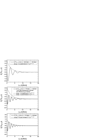
Figure 8: Numerical results for the retarded meson propagator in the two-time representation for a constant mass of 400 MeV, shortly (1 fm/c) after a mass shift to 770 MeV, and a rather long time (about 75 fm/c) after that mass shift. Discussion in the text.

We combine the plots of this propagator with an exponential $\frac{2}{\sqrt{4m^{2}-\Gamma^{2}}}e^{-\frac{1}{2}\Gamma t}$ to show that it decays with the analytically found decay constant. One can also nicely see how the wavelength, related to the mass by $\lambda=\frac{4\pi}{\sqrt{4m^{2}-\Gamma^{2}}}$ (see Eq. (54)), changes with time and that at earlier times in the second plot ($\tau_{2}-t$ large) the frequency still corresponds to masses close to the initial mass and at times close to the present to the final mass. This is a nice illustration of the memory of the retarded propagator and hence the spectral function in the two-time representation. The stronger retardation ($c>2$) for larger changes in the self energy can be explained by considering that the change of the width or mass introduces additional time scales that might as well become of importance such that it is no longer so easy to extract the time scale directly and only from the width.

For the occupation number of the vector mesons, which is basically given by its propagator $G^{<}(\tau,\omega)$ and has to be compared to $G^{<}_{\text{Markov}}(\tau,\omega)=2in_{\text{B}}(T(\tau),\omega)A_{\text{Markov}}(\tau,\omega)$ at time $\tau_{\text{off}}$, we find a by about 50% faster adaption to medium changes: The quantity is not retarded and gains information from the future when Fourier transforming. On the other hand, for the causal dilepton rate (26), which is compared to Eq. (49) with the Bose distribution $n_{\text{B}}(T(\tau),\omega)$ and the spectral function $A_{\text{Markov}}(\tau,\omega)$ at time $\tau_{\text{off}}$, this is not the case: We find a retardation much alike that of the spectral function with similar time scales as given in Eq. (52).

III.4 Quantum interference

As already mentioned, there occurs another interesting effect, arising from the quantum mechanical nature of nonequilibrium dilepton emission. Oscillations in the changing spectral functions, occupation numbers and production rates appear as well as interferences that cannot be present in an approximate semi-classical calculation. The fact that negative values occur temporarily is comparable to the well known observation that the Wigner function, the quantum mechanical analogue to the classical phase space distribution, is not necessarily positive definite (see e.g. Carruthers and Zachariasen (1983)). It is interesting to note that although the rates may oscillate below zero, the total yield will stay positive, being the only physical observable calculated. It can be shown that the accumulated yield is indeed proportional to the square of an amplitude Serreau (2004). The rate in this case is not to be confused with the rate that results from measuring the yield and simply dividing by the time interval. Instead, the rate (26) calculated here has the full quantum mechanical information incorporated and contains interferences that can cause cancellations - in fact, the rate has to be able to become negative. An example for the occurring oscillations is depicted in Fig. 9 for the spectral function and the rate for the case of a mass shift to 400 MeV in the medium at a constant temperature of $175$ MeV. The resulting yield integrated over the time interval beginning with the onset of the changes and ending at the indicated time is shown in Fig. 10. It can be nicely seen that the yield stays positive throughout the evolution while the temporary rate can become negative.

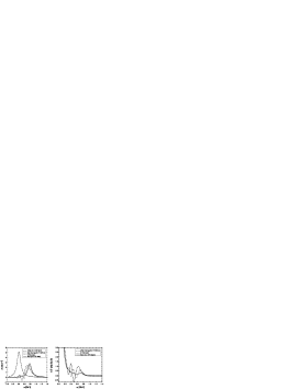
Figure 9: Spectral function and rate for the change of the mass from $m=400$ MeV to 770 MeV (constant $\Gamma$=150 MeV and constant $T=175$ MeV) directly after the self energy has reached its final form (after 7.18 fm/c) and 2 fm/c later. Oscillations and negative values appear in the intermediate spectral functions and rates.

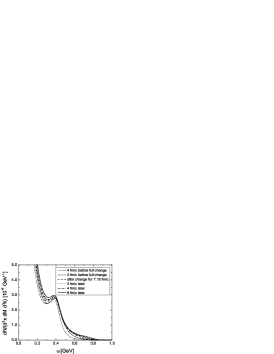
Figure 10: Yields corresponding to rates from Fig. 9 (and some more) integrated over time intervals starting with beginning changes and ending after the indicated duration (3.18 fm/c, 5.18 fm/c, 7.18 fm/c, 9.18 fm/c, 11.18 fm/c and 15.18 fm/c).

III.5 Yields at constant temperature

In order to get a first impression of how memory effects can affect dilepton yields, we investigate yields from systems with a constant size at constant temperature. This helps to understand the more complex situation of an evolving fireball, treated in the next section. For five different scenarios we perform comparisons of the dynamic to the Markovian calculations in that the spectral properties adjust instantaneously to the medium and the dilepton rate has no memory: Modification of the $\rho$-width to $400$ MeV in the medium, shift of the $\rho$-mass using a constant coupling at the $\rho$-$\gamma^{*}$-vertex to $400$ MeV in-medium mass, coupling of the $\rho$ to the N(1520) resonance with and without additional broadening of the resonance and the $\rho$-meson. For the $\omega$-meson we consider a mass-shift by 100 MeV to 682 MeV and broadening to 40 MeV Klingl et al. (1997). We note that the situation for the $\phi$-meson might be similar. In each case the vacuum spectral function is approached linearly within the interval of $7.18$ fm/c, over that we integrate the rates. The temperature is set to $175$ MeV. The results for the first four ($\rho$-meson-) scenarios are shown in Fig. 11. The largest, most noticable difference is found for the mass shift of the $\rho$-meson: The yield from the dynamic calculation is increased by a factor of about 1.8 in the range from 200 to 450 MeV due to the inherent memory integrals. This can be understood since as opposed to the Markov case the spectral function has a certain memory of the in-medium conditions and the stronger weighting of lower masses due to the Bose factor increases the effect additionally.

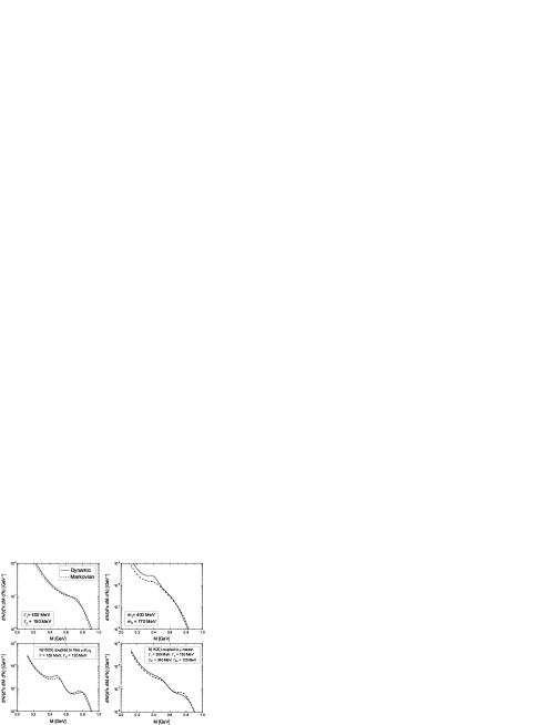
Figure 11: Comparison of the dynamically calculated (solid) to the Markovian (dashed) dilepton yields from an interval of duration $\Delta\tau=7.18$ fm/c in that the self energy was changed linearly from initial to final values given in the figure. Index 1 indicates initial values, index 2 final ones. The temperature was kept constant at $T=175$ MeV.

The other cases show differences, but not as pronounced. We see a minor enhancement of the lower mass tail due to the Bose factor in all cases. This is because for the dynamic case there remains a memory to the larger in-medium width and the resonance peak, giving more strength to the more strongly weighted lower mass part of the distribution than in the Markovian case. In the case of strongly broadened $\rho$-mesons, one can nicely see that the dynamically calculated yield possesses a broader distribution and that for the case of the coupling to the N(1520) without broadening the resonance peak is stronger (by about a factor of 1.5), due to the system’s memory to the coupling in the medium. Here, in the dynamic calculation the vacuum peak is also shifted further to the right due to memory of the level repulsion effect. For the case of coupling to the N(1520) with additional broadening this effect is harder to see because of the very broad distribution - however, the yield around the resonance peak is stronger in this case as well.

For the $\omega$-meson (Fig. 12) large differences show up due to the strong retardation related to the small widths involved. One nicely sees that the in-medium peak is more pronounced in the yield from the dynamic calculation with memory, whereas the final peak is not yet visible. The stronger yield above 800 MeV can be explained by the memory to the larger in-medium width, whereas the decreased yield between 450 and 650 MeV must be due to interferences, discussed in Section III.4. The Bose factor does not have that much influence in this case because the rather small mass shift and broadening do not produce a spectral function with much weight at small frequencies.

To conclude this section we state that for the $\rho$-meson we indeed found noticeable modifications of the yields that one would expect qualitatively when including finite memory for the spectral properties. For the $\omega$-meson, the much longer time scales for the adjustment to the medium further cause structures resulting from quantum mechanical interference after a comparably quick change over 7.18 fm/c.

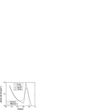
Figure 12: Comparison of the dynamically calculated (solid) to the Markovian (dashed) dilepton yield from $\omega$-mesons from an interval of duration $\Delta\tau=7.18$ fm/c in that the self energy was changed linearly from initial to final values given in the figure. Index 1 indicates initial values, index 2 final ones. The temperature was kept constant at $T=175$ MeV.

III.6 Fireball model and dilepton yields

After having had a first exploration of the influence of finite memory on the dilepton production for constant temperature, we now study a more realistic situation in that memory effects are expected to be of importance. The hadronic phase of a fireball, created in a heavy ion collision, lives for about $\tau_{\text{fireball}}=$ 5 to 10 fm/c at SpS energies. This is the time in that the changes of the vector mesons’ self energy take place, a time comparable to the derived time scale of retardation for the spectral properties and hence the dilepton rate (see Section III.3):

$$\tau_{\text{fireball}}\simeq\bar{\tau}$$ (55)

This is why the consideration of memory effects is important for heavy ion collisions.

We will model the fireball evolution and convolute it with the calculated time dependent rates. We choose for the effective volume a longitudinal Bjorken expansion combined with an accelerating radial flow

$$V_{\text{eff}}(\tau\geq\tau_{0})=\pi c\tau(r_{0}+v_{0}(\tau-\tau_{0})+0.5a_{0}(\tau-\tau_{0})^{2})^{2}\text{,}$$ (56)

with $r_{0}=6.5$ fm, $v_{0}=0.15~{}c$ and $a_{0}=0.05~{}c^{2}/\text{fm}$ (see also Greiner (2003, 2002)). From (56) and the constraint of conserved entropy (given by a constant entropy per baryon $S/A=26$ for SPS energies Greiner et al. (1988); Cleymans et al. (2002); Spieles et al. (1998)), temperature and chemical potentials follow as functions of time. The initial temperature of the fireball is taken slightly above that at chemical freezeout, 175 MeV, whereas the final temperature, reached after a lifetime of about 7.18 fm/c is 120 MeV (thermal freezeout). At this point, we turn off further dilepton production, by decreasing (quasi instantaneously) the temperature towards zero. Afterwards only existing vector mesons decay. We take $A_{\text{B}}=70$ as the number of participant baryons per unit rapidity and include the 56 lightest baryonic and mesonic states in this calculation. Using the calculated time dependent temperature $T(\tau)$ in the computation of the rate and the given volume $V_{\text{eff}}(\tau)$, we can integrate the rate and get the accumulated yield per unit four momentum.

Before this we want to consider the dynamic process of decay, occuring after the production is turned off. Therefore we prepare a situation of constant temperature and fixed spectral properties for the $\rho$-meson and turn down the temperature at a certain point. We then compare the resulting final yield to that calculated analytically for the Markov case using

$$\frac{dN}{d^{3}xd^{4}k}(\tau\rightarrow\infty,\omega)=\frac{dN}{d^{3}xd^{4}k}(\tau_{\text{off}},\omega)+\left(\frac{1}{\Gamma_{\text{final}}}\right)\frac{2e^{4}}{(2\pi)^{5}}\frac{m_{\rho}^{4}}{g_{\rho}^{2}}\frac{1}{\omega^{2}}n_{\text{B}}(T,\omega)\pi A_{\text{Markov}}(\omega)\text{.}$$ (57)

The result is given in Fig. 14. It nicely shows the difference in the decay process: The dynamic calculation leads to a much more pronounced peak while the Markov approximation has larger contributions away from the peak. This can be understood by the investigating the dynamic evolution of the occupation of $\rho$-mesons, given by $D_{\rho}^{<}(\tau,\omega)$, after turning down the temperature. We show this in Fig. 14. It nicely exhibits how the ”thermal” occupation far from the pole mass disappears. This is not given in the approximate Markov formula (Eq. (57)), where $n_{\text{B}}(\omega)$ is constant in time. Integrating the yield over invariant masses $M$ from 125 to 1500 MeV yields the same overall dilepton number for both cases within a percent. Furthermore we find the expected behavior of the dilepton yield integrated over the invariant mass after the time of switching off $\tau_{\text{off}}$: Its increase per unit time decreases with $e^{-\Gamma t}$ (for $t>\tau_{\text{off}}$).

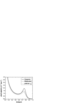
Figure 13: For an equilibrium situation ($\rho$-meson vacuum spectral function and constant temperature) after turning down the temperature, the dynamically calculated yield (solid line) differs from the analytically calculated one (Eq. (57)) (dashed line). Also shown is the yield at time $\tau_{\text{off}}$ from an interval starting 7.18 fm/c before (same for both calculations) (dotted line).

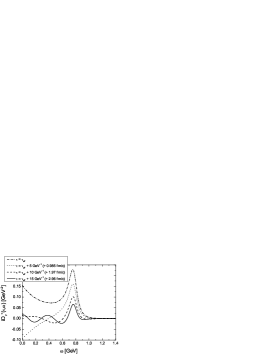
Figure 14: Evolution of $D_{\rho}^{<}(\tau,\omega)$ after having turned off the production at time $\tau_{\text{off}}$.

Now we turn to the situation of an expanding fireball. We consider five different scenarios as in the constant temperature and volume case (see Section III.5): Broadening of the $\rho$-meson to a width of 400 MeV, a mass-shift of the $\rho$-meson to 400 MeV mass, coupling of the $\rho$-meson to the N(1520) resonance with and without broadening, and modification of mass and width of the $\omega$-meson. Comparison to calculations at constant temperature reveals the additional influence of dropping temperature and increasing volume, as well as that of the mentioned difference in behavior to the Markov calculation after the production has been turned off. Overall the differences in the yields are stronger for the case of changing temperature and volume. Fig. 15 shows the comparison to the Markov calculation for the four $\rho$-meson scenarios. There always remains a certain memory of the higher temperatures at earlier times which together with the increasing volume leads to an increased yield within the intermediate mass regime from 400 to 700 MeV for the case of a mass shift to 400 MeV in-medium mass, which was mostly restricted to the vicinity of 400 MeV in the constant temperature case. The dynamically calculated yield around the in-medium peak is now a factor of two larger than that from the Markovian calculation. This constitutes a significant effect and shows the importance of the consideration of the full dynamics for mass shifts, especially if one asks for precise theoretical predictions. In the case of coupling to the N(1520) resonance with and without broadening one now gets more pronounced s-shape structures in the yield than in the Markov case. In addition the different behavior after the temperature was turned off becomes visible in the peak at the vacuum mass. This effect even dominates for the case of the broadened $\rho$-meson such that the actual effect of a broader distribution in the dynamic case, which was seen in the constant temperature calculation, is hidden.

For the situation of a propagating $\omega$-meson mode (Fig. 16) we calculate the final Markovian yield by adding the contribution given in Eq. (57) but using the initial temperature of 175 MeV, since most of the states, populated at high temperature, are still decaying at the time of thermal freeze-out and contribute to the final yield. One can see an enhancement by a factor of more than two between the in-medium mass and about 750 MeV in the dynamic calculation, caused by the finite memory to the in-medium properties. Due to the finite resolution, the numerical treatment can only approximate the narrow $\omega$ vacuum peak and gives visible wiggles in the yield.

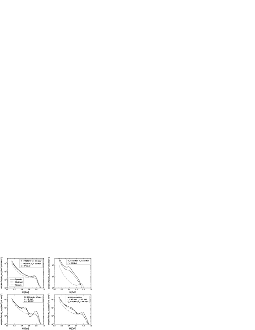
Figure 15: Comparison of the dynamically calculated (solid) to the Markovian (dashed) final dilepton yields where the self energy was changed linearly over an interval of duration $\Delta\tau=7.18$ fm/c as indicated in the corresponding figure (index 1 for initial, 2 for final quantities). The time dependent rate was then convoluted with the temperature and volume of the fireball. Dotted lines show yields from unmodified (vacuum) $\rho$-mesons.

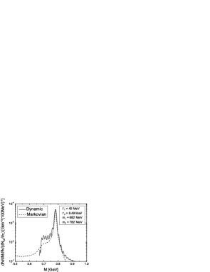
Figure 16: Comparison of the dynamically calculated (solid) to the Markovian (dashed) final dilepton yields for the $\omega$-meson. The self energy was changed linearly over an interval of duration $\Delta\tau=7.18$ fm/c as indicated in the figure (index 1 for initial, 2 for final quantities). The time dependent rate was then convoluted with the temperature and volume of the fireball.

What about the non-zero momentum modes? The shown calculations for the momentum mode $\textbf{k}=0$ can be extrapolated at least to further lower momentum modes, since the self energy is a continuous function with respect to momentum. Typically, for the lowest momenta the strongest medium modifications are seen in experiment Agakishiev et al. (1998, 2005). The yield per unit rapidity and invariant mass can then be given by converting variables and approximating the integral over transverse momenta by a product of the yield for momentum $\textbf{k}=0$ with the regarded momentum range $\Delta\textbf{k}_{\perp}$. In order to get the yield for $y=0$ in the center of mass frame, in the Bjorken model one has to integrate over all rapidities of the fluid cells, using that $y=\eta+y^{\prime}$, where $\eta$ is the space-time rapidity of the cell and $y^{\prime}$ the momentum rapidity of the particles in the restframe of the cell.

$$\left.\frac{dN}{dMdy}\right|_{k_{\perp}<k_{\text{cut}},y=0,\text{CM}} =M\int_{-\infty}^{\infty}d\eta\int_{-\infty}^{\infty}dy^{\prime}\int_{0}^{k_{\text{cut}}}d^{2}k_{\perp}\left(\frac{dN}{dEd^{3}k}\right)_{\text{LR},k_{\parallel}(y^{\prime}),k_{\perp}}\delta(\eta+y^{\prime})$$

$$\approx M\int_{-\infty}^{\infty}d\eta\int_{-\infty}^{\infty}dy^{\prime}\left(\frac{dN}{dEd^{3}k}\right)_{\text{LR},k_{\parallel}(y^{\prime}),k_{\perp}=0}\delta(\eta+y^{\prime})\pi k_{\text{cut}}^{2}$$ (58)

where CM indicates the center of mass frame, LR the local restframe and $k_{\text{cut}}$ is the upper momentum cutoff for transverse momenta. The cutoff $k_{\text{cut}}$ is chosen to be 500 MeV in Agakishiev et al. (1998, 2005) for investigation of dilepton yields for lower transverse momenta. For the Bjorken model we encounter the problem that arbitrarily large rapidities $y^{\prime}$ and hence also large longitudinal momenta contribute. Approximating the yields for these momentum modes by that for $\textbf{k}=0$ is not reasonable.

On the other hand for a ”semi-static” expanding fireball model as employed in e.g. Rapp and Wambach (2000, 1999) the situation becomes much simpler as in this case the only dilepton longitudinal momentum contributing to the midrapidity yield is $k_{\parallel}=0$ and we have

$$\left.\frac{dN}{dMdy}\right|_{k_{\perp}<k_{\text{cut}},y=0} =M\int_{0}^{k_{\text{cut}}}d^{2}k_{\perp}\left(\frac{dN}{dEd^{3}k}\right)_{k_{\parallel}=0,k_{\perp}}$$

$$\approx M\left(\frac{dN}{dEd^{3}k}\right)_{k_{\parallel}=0,k_{\perp}=0}\pi k^{2}_{\text{cut}}\text{.}$$ (59)

No momenta larger than $k_{\text{cut}}$ are involved for this case and one can approximate the yields for the appearing small momenta by those for zero momentum. Hence also for measurable finite momentum intervals the resulting modifications of the yields due to finite memory are expected to be completely similar and our primary message remains valid.

We summarize by stating that inclusion of the fireball evolution leads to further enhancement of the differences between the dilepton yields calculated using a full nonequilibrium quantum field theoretical formulation including retardation and its much simpler Markovian approximation. For the realistic situation of a heavy ion collision memory effects have to be considered when it comes to predicting medium modifications of particles.

IV Summary and Conclusions

In the present work, we have numerically calculated dilepton production rates within a nonequilibrium field theory formalism, based on the real time approach of Schwinger and Keldysh Schwinger (1961); Keldysh (1964, 1965); Craig (1968). We employed the Kadanoff-Baym equations, generalized to the relativistic Dirac structure, to derive the formula for the dilepton production rate, which is non-local in time and hence includes the usually disregarded finite memory. The rate is in principle a (half) Fourier transform over past times of the virtual photon occupation, described by the Green function $D_{\gamma}^{<}$ in the two-time representation. Medium modifications of the vector mesons enter this production rate via the virtual photon’s self energy that is connected to the vector meson propagator by the principle of vector meson dominance.

The equation of motion for the retarded and advanced vector meson propagator also followed from the Kadanoff-Baym equations. From its solution it was possible to extract the dynamic behavior of the meson’s spectral function and to define a time scale on that it adjusts to medium changes, which were incorporated by the definition of a time dependent self energy for the vector mesons. This time scale was found to be proportional to the inverse vacuum width of the meson like $c/\Gamma$. $c$ lies between $2$ and about $3.5$. The time that the dilepton rate needs to follow changes was found to be approximately equal to that for the spectral function. Since these time scales lie in the range of typical times in that the hadronic phase of fireballs in heavy ion reactions exists and evolves, we expected an influence of the found retardation on the dilepton yields and investigated different scenarios quantitatively. Possible medium modifications of the vector mesons, as shifted pole masses, motivated by Brown-Rho scaling, broadening and coupling to resonance-hole pairs were considered. Investigation of the dynamical off-shell evolution of the spectral function, meson occupation number and resulting dilepton rate revealed the quantum mechanical nature of the system, manifested in appearing oscillations and hence interferences in the regarded quantities after changes of the self energy that were fast as compared to the derived time scales. All quantities were found to possibly become negative, which is a major difference to the Markov approximation within which all quantities are always positive definite. The oscillations potentially cancel when the rate is integrated over time such that the measurable dilepton yield is found to be positive, as it has to be. On the other hand, for situations where the particular rate can become negative, a semi-classical interpretation with positive definite rates, as employed in present day transport codes, is not possible.

We first calculated dilepton yields from a time dependent system at constant volume and temperature considering different possible medium modifications and compared to the yields found assuming an instantaneous (Markovian) adjustment of all quantities to the medium. For the $\rho$-meson we found qualitatively expected results for each case. Quantitatively, the strongest difference in the differently calculated yields appeared for the case of a mass shift to 400 MeV in-medium mass, as suggested by Brown-Rho scaling. This is due to the stronger weighting of the lower masses by the Bose factor and since the spectral function moves more slowly towards the free mass in the dynamic situation, we found more enhancement in the yield than for the Markov calculation without memory. It was shown that there can be more than a factor of two difference. For the medium modified $\omega$-meson the qualitatively expected results plus additional structures caused by quantum interferences were seen. These are stronger than in the case of the $\rho$-meson because the performed change is faster relative to the time scale for adiabatic behavior of the $\omega$-meson, which has a very small width.

The introduction of a fireball model allowed us to perform more realistic simulations including changing temperature and volume, adjusted to the case of the SpS with energies of 158 AGeV. The modifications of the yields due to inclusion of finite memory were enhanced as compared to the constant temperature case. Also the behavior of the regarded quantities after freeze-out was revealed to be different from that assumed in Markovian calculations. For the mass shift of the $\rho$-meson a factor of two difference in the two calculated yields was found around the in-medium mass - a significant effect. For the case of substantial broadening without further modifications, the differences are only very small. In all scenarios, also for the $\omega$-meson, lower invariant masses were slightly enhanced in the dynamic calculation. For the coupling to the N(1520) resonance the peaks were more pronounced than in the Markov calculation.

In summary, our findings show that exact treatment of medium modifications of particles in relativistic heavy ion collisions requires the consideration of memory effects. This is in particular true for mass shifts or the occurrence of two-peak structures in their spectral properties. It has to be a future task to find how to incorporate such memory effects in semi-classical transport simulations. This should be also of relevance for the description of production and propagation of vector mesons through cold nuclei in photo-nuclear reactions Muhlich et al. (2003, 2004).

Acknowledgments

The authors thank Stefan Leupold and Marcus Post for helpful discussions throughout this work.

Appendix A On the acausality of the Kadanoff-Baym parametrization

In this appendix we first show that the choice of time variables $\tau_{\text{KB}}=\frac{t_{\alpha}+t_{\beta}}{2}$ and $\Delta t=t_{\alpha}-t_{\beta}$ leads to an acausal spectral function $A(\tau_{\text{KB}},\omega)$. This choice will be referred to as the Kadanoff-Baym parametrization since it was first introduced by Kadanoff and Baym in Kadanoff and Baym (1962) for a first order gradient expansion of the full quantum transport equations. We introduce a different parametrization $\tau=t_{\alpha}$ and $\Delta t=t_{\alpha}-t_{\beta}$ and obtain a spectral function $A(\tau,\omega)$ that has no information on the future incorporated.

The following analysis of the differential equation of the retarded propagator

$$\hat{D}_{t_{A}}D_{\rho}^{\text{ret}}(t_{A},t_{B})=\int_{t_{B}}^{t_{A}}dt_{2}\Sigma_{\rho}^{\text{ret}}(t_{A},t_{2})D_{\rho}^{\text{ret}}(t_{2},t_{B})$$ (60)

allows us to find the times, from which medium information $\Sigma^{\text{ret}}(t_{1},t_{2})$ is contributed to $D_{\rho}^{\text{ret}}(t_{A},t_{B})$.

$D_{\rho}^{\text{ret}}(t_{A},t_{B})$ follows by integration of $\hat{D}_{t_{1}}D_{\rho}^{\text{ret}}(t_{1},t_{B})=\int_{t_{B}}^{t_{1}}dt_{2}\Sigma_{\rho}^{\text{ret}}(t_{1},t_{2})D_{\rho}^{\text{ret}}(t_{2},t_{B})$ over $t_{1}\epsilon[t_{B},t_{A}]$, starting at $t_{1}=t_{B}$. Since all quantities are retarded, we always have $t_{A}\geq t_{1}\geq t_{2}\geq t_{B}$. $D_{\rho}^{\text{ret}}(t_{1},t_{B})$ itself has contributions from $D_{\rho}^{\text{ret}}(t_{2},t_{B})$ and $\Sigma_{\rho}^{\text{ret}}(t_{1},t_{2})$ with $t_{2}\epsilon[t_{B},t_{1}]$. Fig. 18 schematically shows where in time these contributions are located. On the horizontal line enter contributions from $\Sigma_{\rho}^{\text{ret}}(t_{1},t_{2})$, on the vertical line those from $D_{\rho}^{\text{ret}}(t_{2},t_{B})$. After integration over $t_{1}\epsilon[t_{B},t_{A}]$, one finds that $D_{\rho}^{\text{ret}}(t_{A},t_{B})$ is created solely with information $\Sigma_{\rho}^{\text{ret}}(t_{1},t_{2})$, defined at times lying in the triangle shown in Fig. 18.

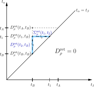
Figure 17: (Color online) Ranges in time (shaded regions) that contribute to $D_{\rho}^{\text{ret}}(t_{1},t_{B})$ in the $t_{\alpha}$-$t_{\beta}$-plane, where $t_{\alpha}$ ($t_{\beta}$) stands for the first (second) time argument.

Figure 18: (Color online) Contributions of $\Sigma^{\text{ret}}(t_{\alpha}$, $t_{\beta})$ to $D_{\rho}^{\text{ret}}(t_{A},t_{B})$ come from times $t_{\alpha}$, $t_{\beta}$, lying within the shaded region.

When we now choose to transform time variables like $\tau_{\text{KB}}=\frac{t_{\alpha}+t_{\beta}}{2}$ and $\Delta t=t_{\alpha}-t_{\beta}$, we find that the Green function $D_{\rho}^{\text{ret}}(\tau_{\text{KB}},\Delta t)$ is created also with information defined in its future as demonstrated in Fig. 20. Hence, this parametrization cannot be causal and is not suitable for finding appropriate time scales for adaption of the spectral function to medium changes in time. The spectral function $A(\tau_{\text{KB}},\omega)=-\frac{1}{\pi}\text{Im}D_{\rho}^{\text{ret}}(\tau_{\text{KB}},\omega)$ is the imaginary part of the Fourier transform in relative time coordinates of the Green function and hence would have incorporated information on self energies from the future.

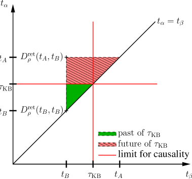
Figure 19: (Color online) After transformation to $\tau_{\text{KB}}=\frac{t_{\alpha}+t_{\beta}}{2}$ and $\Delta t=t_{\alpha}-t_{\beta}$ the Green function at time $\tau_{\text{KB}}=\frac{t_{A}+t_{B}}{2}$, $D_{\rho}^{\text{ret}}(\tau_{\text{KB}},\Delta t)$, has contributions of $\Sigma^{\text{ret}}(t_{\alpha}$, $t_{\beta})$ also from its future, indicated by the upper shaded region.

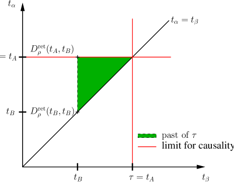
Figure 20: (Color online) Choosing the parametrization $\tau=t_{\alpha}$ and $\Delta t=t_{\alpha}-t_{\beta}$ leads to a Green function $D_{\rho}^{\text{ret}}(\tau=t_{A},\Delta t)$ without contributions of $\Sigma^{\text{ret}}(t_{\alpha}$, $t_{\beta})$ from the future.

On the other hand, using $\tau=t_{\alpha}$ and $\Delta t=t_{\alpha}-t_{\beta}$, as done throughout this work, the situation looks as depicted in Fig. 20. Only past times contribute to the Green function at time $\tau=t_{A}$. A spectral function defined as $A(t_{\alpha},\omega)=-\frac{1}{\pi}\text{Im}D_{\rho}^{\text{ret}}(t_{\alpha},\omega)$ is causal as required.

References

- Rapp and Wambach (2000) R. Rapp and J. Wambach, Adv. Nucl. Phys. 25, 1 (2000), eprint hep-ph/9909229.
- Agakishiev et al. (1995) G. Agakishiev et al. (CERES), Phys. Rev. Lett. 75, 1272 (1995).
- Agakishiev et al. (1998) G. Agakishiev et al. (CERES/NA45), Phys. Lett. B422, 405 (1998), eprint nucl-ex/9712008.
- Effenberger et al. (1999) M. Effenberger, E. L. Bratkovskaya, and U. Mosel, Phys. Rev. C60, 044614 (1999), eprint nucl-th/9903026.
- Effenberger and Mosel (1999) M. Effenberger and U. Mosel, Phys. Rev. C60, 051901 (1999), eprint nucl-th/9906085.
- Cassing and Juchem (2000a) W. Cassing and S. Juchem, Nucl. Phys. A665, 377 (2000a), eprint nucl-th/9903070.
- Cassing and Juchem (2000b) W. Cassing and S. Juchem, Nucl. Phys. A672, 417 (2000b), eprint nucl-th/9910052.
- Cassing and Juchem (2000c) W. Cassing and S. Juchem, Nucl. Phys. A677, 445 (2000c), eprint nucl-th/0003002.
- Leupold (2000) S. Leupold, Nucl. Phys. A672, 475 (2000), eprint nucl-th/9909080.
- Leupold (2001) S. Leupold, Nucl. Phys. A695, 377 (2001), eprint nucl-th/0008036.
- Larionov et al. (2002) A. B. Larionov, M. Effenberger, S. Leupold, and U. Mosel, Phys. Rev. C66, 054604 (2002), eprint nucl-th/0107031.
- Juchem et al. (2004a) S. Juchem, W. Cassing, and C. Greiner, Phys. Rev. D69, 025006 (2004a), eprint hep-ph/0307353.
- Berges and Cox (2001) J. Berges and J. Cox, Phys. Lett. B517, 369 (2001), eprint hep-ph/0006160.
- Berges et al. (2003) J. Berges, S. Borsanyi, and J. Serreau, Nucl. Phys. B660, 51 (2003), eprint hep-ph/0212404.
- Aarts and Berges (2001) G. Aarts and J. Berges, Phys. Rev. D64, 105010 (2001), eprint hep-ph/0103049.
- Juchem et al. (2004b) S. Juchem, W. Cassing, and C. Greiner, Nucl. Phys. A743, 92 (2004b), eprint nucl-th/0401046.
- Rapp and Wambach (1999) R. Rapp and J. Wambach, Eur. Phys. J. A6, 415 (1999), eprint hep-ph/9907502.
- Cassing and Bratkovskaya (1999) W. Cassing and E. L. Bratkovskaya, Phys. Rept. 308, 65 (1999).
- Wang and Boyanovsky (2001) S.-Y. Wang and D. Boyanovsky, Phys. Rev. D63, 051702 (2001), eprint hep-ph/0009215.
- Wang et al. (2002) S.-Y. Wang, D. Boyanovsky, and K.-W. Ng, Nucl. Phys. A699, 819 (2002), eprint hep-ph/0101251.
- Boyanovsky and de Vega (2003) D. Boyanovsky and H. J. de Vega, Phys. Rev. D68, 065018 (2003), eprint hep-ph/0305224.
- Boyanovsky and de Vega (2005) D. Boyanovsky and H. J. de Vega, Nucl. Phys. A747, 564 (2005), eprint hep-ph/0311156.
- Schwinger (1961) J. S. Schwinger, J. Math. Phys. 2, 407 (1961).
- Keldysh (1964) L. Keldysh, Zh. Eks. Teor. Fiz. 47, 1515 (1964).
- Keldysh (1965) L. Keldysh, Sov. Phys. JETP 20, 1018 (1965).
- Craig (1968) R. Craig, J. Math. Phys. 9, 605 (1968).
- Kadanoff and Baym (1962) L. Kadanoff and G. Baym, Quantum Statistical Mechanics (Benjamin, New York, 1962).
- Brown and Rho (1991) G. E. Brown and M. Rho, Phys. Rev. Lett. 66, 2720 (1991).
- Cooper (1999) F. Cooper, Phys. Rept. 315, 59 (1999), eprint hep-ph/9811246.
- Serreau (2004) J. Serreau, JHEP 05, 078 (2004), eprint hep-ph/0310051.
- Bjorken and Drell (1965) J. Bjorken and S. Drell, Relativistic Quantum Fields (MacGraw-Hill, New York, 1965).
- Greiner et al. (1994) C. Greiner, K. Wagner, and P. G. Reinhard, Phys. Rev. C49, 1693 (1994).
- Bezzerides and DuBois (1972) B. Bezzerides and D. F. DuBois, Ann.Phys. 70, 10 (1972).
- Botermans and Malfliet (1990) W. Botermans and R. Malfliet, Phys. Rept. 198, 115 (1990).
- Mrowczynski and Heinz (1994) S. Mrowczynski and U. W. Heinz, Ann. Phys. 229, 1 (1994).
- Danielewicz (1984) P. Danielewicz, Annals Phys. 152, 305 (1984).
- Greiner and Leupold (1998) C. Greiner and S. Leupold, Annals Phys. 270, 328 (1998), eprint hep-ph/9802312.
- McLerran and Toimela (1985) L. D. McLerran and T. Toimela, Phys. Rev. D31, 545 (1985).
- Weldon (1990) H. A. Weldon, Phys. Rev. D42, 2384 (1990).
- Gale and Kapusta (1991) C. Gale and J. I. Kapusta, Nucl. Phys. B357, 65 (1991).
- Kubo (1957) R. Kubo, J. Phys. Soc. Japan 12, 570 (1957).
- Martin and Schwinger (1959) P. C. Martin and J. S. Schwinger, Phys. Rev. 115, 1342 (1959).
- Sakurai (1960) J. J. Sakurai, Annals Phys. 11, 1 (1960).
- Sakurai (1969) J. Sakurai, Currents and Mesons (University of Chicago Press, Chicago, 1969).
- Kroll et al. (1967) N. M. Kroll, T. D. Lee, and B. Zumino, Phys. Rev. 157, 1376 (1967).
- Peters et al. (1998) W. Peters, M. Post, H. Lenske, S. Leupold, and U. Mosel, Nucl. Phys. A632, 109 (1998), eprint nucl-th/9708004.
- Henning (1995) P. A. Henning, Nucl. Phys. A582, 633 (1995), eprint hep-ph/9402306.
- Herrmann et al. (1992) M. Herrmann, B. L. Friman, and W. Noerenberg, Nucl. Phys. A545, 267c (1992).
- Chanfray and Schuck (1992) G. Chanfray and P. Schuck, Nucl. Phys. A545, 271c (1992).
- Rapp et al. (1996) R. Rapp, G. Chanfray, and J. Wambach, Phys. Rev. Lett. 76, 368 (1996), eprint hep-ph/9508353.
- Friman and Pirner (1997) B. Friman and H. J. Pirner, Nucl. Phys. A617, 496 (1997), eprint nucl-th/9701016.
- Klingl et al. (1997) F. Klingl, N. Kaiser, and W. Weise, Nucl. Phys. A624, 527 (1997), eprint hep-ph/9704398.
- Post et al. (2004) M. Post, S. Leupold, and U. Mosel, Nucl. Phys. A741, 81 (2004), eprint nucl-th/0309085.
- Henning and Umezawa (1994) P. A. Henning and H. Umezawa, Nucl. Phys. A571, 617 (1994), eprint nucl-th/9304005.
- Eidelman et al. (2004) S. Eidelman et al. (Particle Data Group PDG), Physics Letters B 592, 010001 (2004).
- Carruthers and Zachariasen (1983) P. Carruthers and F. Zachariasen, Rev. Mod. Phys. 55, 245 (1983).
- Greiner (2003) C. Greiner, AIP Conf. Proc. 644, 337 (2003), eprint nucl-th/0208080.
- Greiner (2002) C. Greiner, J. Phys. G28, 1631 (2002), eprint nucl-th/0112080.
- Greiner et al. (1988) C. Greiner, D.-H. Rischke, H. Stocker, and P. Koch, Phys. Rev. D38, 2797 (1988).
- Cleymans et al. (2002) J. Cleymans, B. Kaempfer, and S. Wheaton, Phys. Rev. C65, 027901 (2002), eprint nucl-th/0110035.
- Spieles et al. (1998) C. Spieles, H. Stocker, and C. Greiner, Eur. Phys. J. C2, 351 (1998), eprint nucl-th/9704008.
- Agakishiev et al. (2005) G. Agakishiev et al. (CERES), Eur. Phys. J. C41, 475 (2005).
- Muhlich et al. (2003) P. Muhlich et al., Phys. Rev. C67, 024605 (2003), eprint nucl-th/0210079.
- Muhlich et al. (2004) P. Muhlich, T. Falter, and U. Mosel, Eur. Phys. J. A20, 499 (2004), eprint nucl-th/0310067.