Fine and hyperfine structure
in different bound systems

Abstract

We demonstrate that the generalized Gell-Mann–Low theorem permits for a systematic expansion around the nonrelativistic limit when applied to bound states in the Wick-Cutkosky model, Yukawa theory, and QED (in Coulomb gauge). We apply this expansion to obtain new results for the fine and hyperfine structure of bound states in the cases of the Wick-Cutkosky model and Yukawa theory, and reproduce correctly the fine and hyperfine structure of hydrogenic systems.

1 Introduction

In this paper we present a method to extract the fine and hyperfine structure, presently to lowest order, of bound systems appearing in general relativistic quantum field theories in a systematic, consistent and transparent way. It is based on the application of a generalization of the Gell-Mann–Low theorem [1] which generates an effective Hamiltonian called the Bloch-Wilson Hamiltonian, for the dynamics of the two constituents. The Bloch-Wilson Hamiltonian consists of the relativistic kinetic energy of the constituents and an effective potential that can be obtained explicitly in a perturbative expansion in powers of the coupling constant, derived from the Dyson series for the adiabatic evolution operator. At every perturbative order, the effective potential can be expanded in powers of the relative momentum, which, together with the corresponding expansion of the relativistic kinetic energy, leads to a systematic expansion around the nonrelativistic limit.

We will demonstrate this procedure in three different theories, a scalar model with cubic couplings (the “Wick-Cutkosky model”), Yukawa theory, and quantum electrodynamics (QED). The Bloch-Wilson Hamiltonian for two of these theories has been carefully derived to lowest nontrivial order (in the expansion in powers of the coupling constant) and used for numerical bound state calculations before [2, 3]. The Bloch-Wilson Hamiltonian for QED in the Coulomb gauge has been discussed very briefly in Ref. [4], and will be treated in much more detail in a future publication. In each case, we will take the exchanged boson to be massless in order to have analytic expressions in the nonrelativistic limit and for the lowest-order fine and hyperfine structure.

This procedure should be compared with the historical calculation of the complete fine and hyperfine structure in hydrogenic systems. Ref. [5] gives a good overview of these calculations which are based on the Breit equation [6] and have not been completed until 1951. A more systematic treatment is provided by the Bethe-Salpeter equation [7, 8] in the perturbative expansion devised by Salpeter [9]. However, Salpeter’s expansion begins at zero order with an instantaneous interaction of the constituents which is natural in QED, particularly in the Coulomb gauge, but not in the case of spinless boson exchange as in the Wick-Cutkosky model and Yukawa theory. In fact, the analogue in the Bethe-Salpeter approach to the procedure outlined above would be to consider the lowest-order approximation to the Bethe-Salpeter kernel, the so-called ladder approximation, and expand the equation in this approximation around the nonrelativistic limit. However, even in the simplest case of the Wick-Cutkosky model [10] this procedure leads to a “curious” term of the unexpected order $\alpha^{3}\ln\alpha$ [11]. The full fine structure in this model and in Yukawa theory have, to our knowledge, never been calculated.

In the next two sections of this paper, we will present the Bloch-Wilson Hamiltonians for the field theories mentioned above. In fact, we will discuss two different types of effective Hamiltonians, in Section 2 the Bloch-Wilson Hamiltonian used before in Refs. [2, 3, 4] which generalizes in a natural way Bloch’s formulation of degenerate perturbation theory [12], and in Section 3 a hermitian version used before by Wilson [13] and, independently, by Gari et al. [14] and by Krüger and Glöckle [15], building on earlier work by Okubo [16]. As will become clear in Section 4, the two types of effective Hamiltonians differ by an antihermitian term in the expansion around the nonrelativistic limit which is present in the first type of effective Hamiltonians (except for the case of QED) but obviously not in the second. In Section 4, we will describe how to calculate the fine and hyperfine structure to lowest order starting from these effective Hamiltonians, relegating the more technical aspects of the calculations to Appendix A. In particular, we will use second-order time-independent perturbation theory to calculate the contributions originating from the antihermitian term. An alternative method based on a Foldy-Wouthuysen-type transformation from a nonhermitian to a hermitian Hamiltonian is detailed in Appendix B. We will also comment on the possible physical significance of the antihermitian term. In Section 5, we discuss the results for the fine and hyperfine structure in the different theories and compare in particular with the numerical solutions [2, 3] for the Bloch-Wilson Hamiltonian (to lowest nontrivial order in the expansion in powers of the coupling constant) without the expansion around the nonrelativistic limit, and with the well-known fine and hyperfine structure in hydrogenic systems.

2 The Bloch-Wilson Hamiltonian

We will begin by stating the generalization of the Gell-Mann–Low theorem proved in Ref. [1]. To this end, some general notations have to be introduced first: the full Hamiltonian $H$ of the field theory under consideration is decomposed into a “free” Hamiltonian $H_{0}$ (typically the one describing free particles) and an interaction Hamiltonian $H_{1}$, $H=H_{0}+H_{1}$. The adiabatic evolution operator $U_{\epsilon}$ maps a state $|\phi\rangle$ in the Fock space $\mathcal{F}$ in which $H_{0}$ acts, to the state $|\psi\rangle$ that results from evolving $|\phi\rangle$ with the Schrödinger equation corresponding to the adiabatic Hamiltonian

$$H_{\epsilon}(t)=H_{0}+e^{-\epsilon\lvert t\rvert}H_{1}\>,\qquad\epsilon>0\>,$$ (1)

from $t\to-\infty$ to $t=0$. The adiabatic evolution operator has the perturbative expansion

$$U_{\epsilon}=\sum_{n=0}^{\infty}\frac{(-i)^{n}}{n!}\int_{-\infty}^{0}dt_{1}\cdots\int_{-\infty}^{0}dt_{n}\,e^{-\epsilon(\lvert t_{1}\rvert+\ldots+\lvert t_{n}\rvert)}\,T[H_{1}(t_{1})\cdots H_{1}(t_{n})]\>,$$ (2)

the well-known Dyson series, where

$$H_{1}(t)=e^{iH_{0}t}H_{1}\,e^{-iH_{0}t}\>.$$ (3)

For the generalized Gell-Mann–Low theorem, a linear $H_{0}$-invariant subspace $\Omega_{0}\subseteq\mathcal{F}$, $H_{0}\Omega_{0}\subseteq\Omega_{0}$, is fixed and the corresponding orthogonal projection operator $P_{0}:\mathcal{F}\to\Omega_{0}$ introduced. The theorem asserts that, if the operator

$$U_{B}=\lim_{\epsilon\to 0}\,U_{\epsilon}(P_{0}U_{\epsilon}P_{0})^{-1}:\Omega_{0}\to U_{B}(\Omega_{0})\equiv\Omega\>,$$ (4)

the Bloch-Wilson operator, is well-defined in $\Omega_{0}$, then the image subspace $\Omega$ is invariant under $H$, $H\Omega\subseteq\Omega$. By its definition, $U_{B}$ is “normalized” to

$$P_{0}U_{B}=\mathbf{1}_{\Omega_{0}}=\left.P_{0}\right|_{\Omega_{0}}\>,$$ (5)

consequently the inverse of $U_{B}$ is $\left.P_{0}\right|_{\Omega}$. This normalization naturally generalizes the one used in the original Gell-Mann–Low theorem [8] and corresponds to the one used by Bloch in his formulation of degenerate perturbation theory [12]. Note that we have changed the notation for the Bloch-Wilson operator compared to our previous works to emphasize this fact, for reasons to become clear later. The existence of the operator $U_{B}$ and the assertion of the theorem are to be understood order by order in the corresponding formal power series originating from Eq. (2), as is the case for the original Gell-Mann–Low theorem.

The fact that $\Omega$ is $H$-invariant is equivalent to the diagonalizability of $H$ in $\Omega$, so that part of the eigenvalue problem of $H$ can be solved in $\Omega$. It is convenient to similarity transform the eigenvalue problem back from $\Omega$ to the usually more manageable subspace $\Omega_{0}$. Hence we define the effective or Bloch-Wilson Hamiltonian

$$H_{B}=P_{0}HU_{B}:\Omega_{0}\to\Omega_{0}\>.$$ (6)

We can use Eq. (5) and $P_{0}H_{0}=H_{0}P_{0}$ as a consequence of the $H_{0}$-invariance of $\Omega_{0}$, to bring $H_{B}$ into the form

$$H_{B} =P_{0}H_{0}U_{B}+P_{0}H_{1}U_{B}$$

$$=H_{0}P_{0}+P_{0}H_{1}U_{B}\>.$$ (7)

The eigenvalue problem of $H_{B}$ in $\Omega_{0}$ is equivalent to the one of $H$ restricted to $\Omega$ with the identical eigenvalues. The corresponding eigenstates are mapped into each other by $U_{B}$ and $P_{0}$.

For the following bound state calculations we will take $\Omega_{0}$ to be the subspace of all states of the constituents as free particles (under $H_{0}$), usually in a momentum eigenstate basis. In this case, the first part $H_{0}P_{0}$ in Eq. (7) just represents the kinetic energy of the constituents, consequently the second part defines an effective potential for their interaction (although it also contains radiative corrections to the vacuum energy and the masses of the constituents) given in terms of a power series in the coupling constant by inserting the Dyson series (2). The operator $P_{0}$ projects out from the true $H$-eigenstates in $\Omega$ the component with the particle numbers corresponding to the constituents, hence we can think of the corresponding $H_{B}$-eigenstates as wave functions of the constituents, the higher Fock space components (with higher particle numbers) being generated by the application of $U_{B}$. For bound states, it is these constituent wave functions that have to be normalizable, while the corresponding $H$-eigenstates will usually not be normalizable with respect to the standard Fock space scalar product.

In the following, we will calculate $H_{B}$ to lowest nontrivial order for two-particle subspaces. In all field theories to be considered, the interaction Hamiltonian $H_{1}$ changes the particle number so that

$$P_{0}H_{1}(t)P_{0}=0\>.$$ (8)

In this case, the lowest-order nontrivial contribution to $H_{B}$ arises from the first-order term in the expansion (2), and we can write

$$H_{B}=H_{0}P_{0}-i\int_{-\infty}^{0}dt\,e^{-\epsilon\lvert t\rvert}P_{0}H_{1}(0)H_{1}(t)P_{0}+\mathcal{O}(H_{1}^{4})\>,$$ (9)

where the limit $\epsilon\to 0$ is understood.

2.1 Wick-Cutkosky model

We will now present the Bloch-Wilson Hamiltonian $H_{B}$ for three different theories. We start with the “Wick-Cutkosky model”, a field theory with three scalar fields $\phi_{A}$, $\phi_{B}$, and $\varphi$, the latter taken to be massless, with interaction Hamiltonian

$$H_{1}=g\int d^{3}x\bm{:}\left[\phi_{A}^{\dagger}(\mathbf{x})\phi_{A}(\mathbf{x})+\phi_{B}^{\dagger}(\mathbf{x})\phi_{B}(\mathbf{x})\right]\varphi(\mathbf{x})\bm{:}\>.$$ (10)

We consider states with one $A$ and one $B$ scalar. The Bloch-Wilson Hamiltonian for the corresponding subspace was calculated in Ref. [2], with matrix elements

$$\langle\mathbf{p}_{A},\mathbf{p}_{B}|H_{B}|\mathbf{p}_{A}^{\prime},\mathbf{p}_{B}^{\prime}\rangle =\left(\sqrt{m_{A}^{2}+\mathbf{p}_{A}^{2}}+\sqrt{m_{B}^{2}+\mathbf{p}_{B}^{2}}\right)(2\pi)^{3}\delta(\mathbf{p}_{A}-\mathbf{p}_{A}^{\prime})(2\pi)^{3}\delta(\mathbf{p}_{B}-\mathbf{p}_{B}^{\prime})$$

$$\phantom{=}-\frac{g^{2}}{\sqrt{2E_{\mathbf{p}_{A}}^{A}\,2E_{\mathbf{p}_{B}}^{B}\,2E_{\mathbf{p}_{A}^{\prime}}^{A}\,2E_{\mathbf{p}_{B}^{\prime}}^{B}}}$$

$$\phantom{=}\times\frac{1}{2\lvert\mathbf{p}_{A}-\mathbf{p}_{A}^{\prime}\rvert}\left(\frac{1}{E_{\mathbf{p}_{A}}^{A}+\lvert\mathbf{p}_{A}-\mathbf{p}_{A}^{\prime}\rvert-E_{\mathbf{p}_{A}^{\prime}}^{A}}+\frac{1}{E_{\mathbf{p}_{B}}^{B}+\lvert\mathbf{p}_{B}-\mathbf{p}_{B}^{\prime}\rvert-E_{\mathbf{p}_{B}^{\prime}}^{B}}\right)$$

$$\phantom{=}\hskip 142.26378pt\times(2\pi)^{3}\delta(\mathbf{p}_{A}+\mathbf{p}_{B}-\mathbf{p}_{A}^{\prime}-\mathbf{p}_{B}^{\prime})$$ (11)

in a momentum eigenstate basis with the nonrelativistic normalization

$$\langle\mathbf{p}_{A},\mathbf{p}_{B}|\mathbf{p}_{A}^{\prime},\mathbf{p}_{B}^{\prime}\rangle=(2\pi)^{3}\delta(\mathbf{p}_{A}-\mathbf{p}_{A}^{\prime})(2\pi)^{3}\delta(\mathbf{p}_{B}-\mathbf{p}_{B}^{\prime})\>.$$ (12)

We have introduced the shorthands

$$E_{\mathbf{p}}^{A,B}=\sqrt{m_{A,B}^{2}+\mathbf{p}^{2}}$$ (13)

for the relativistic kinetic energies in Eq. (11). To arrive at the form (11), the vacuum energy (including its lowest-order radiative corrections) was subtracted, and radiative corrections to the kinetic energy have been absorbed in a renormalization of the masses. The renormalization procedure was analyzed in detail in Ref. [3] from the present not manifestly covariant point of view, and the appearing one- and two-loop expressions have been shown to coincide with the ones of usual covariant perturbation theory. The renormalized masses are denoted here as $m_{A,B}$. Making use of the overall momentum conservation $\mathbf{p}_{A}+\mathbf{p}_{B}=\mathbf{p}_{A}^{\prime}+\mathbf{p}_{B}^{\prime}$, the dynamics can be reduced to the center-of-mass system $\mathbf{p}_{A}+\mathbf{p}_{B}=\mathbf{0}$. One then has for the corresponding Schrödinger equation, with ${\mathbf{p}}={\mathbf{p}}_{A}=-{\mathbf{p}}_{B}$,

$$\left(\sqrt{m_{A}^{2}+\mathbf{p}^{2}}+\sqrt{m_{B}^{2}+\mathbf{p}^{2}}\right)\phi(\mathbf{p})-\frac{g^{2}}{\sqrt{2E_{\mathbf{p}}^{A}\,2E_{\mathbf{p}}^{B}}}\int\frac{d^{3}p^{\prime}}{(2\pi)^{3}}\,\frac{1}{\sqrt{2E_{\mathbf{p}^{\prime}}^{A}\,2E_{\mathbf{p}^{\prime}}^{B}}}\,\\ \times\frac{1}{2\lvert\mathbf{p}-\mathbf{p}^{\prime}\rvert}\left(\frac{1}{E_{\mathbf{p}}^{A}+\lvert\mathbf{p}-\mathbf{p}^{\prime}\rvert-E_{\mathbf{p}^{\prime}}^{A}}+\frac{1}{E_{\mathbf{p}}^{B}+\lvert\mathbf{p}-\mathbf{p}^{\prime}\rvert-E_{\mathbf{p}^{\prime}}^{B}}\right)\phi(\mathbf{p}^{\prime})=E\phi(\mathbf{p})\>,$$ (14)

with the wave function $\phi(\mathbf{p})$ defined as

$$\langle\mathbf{p}_{A},\mathbf{p}_{B}|\phi\rangle=\phi(\mathbf{p}_{A})(2\pi)^{3}\delta(\mathbf{p}_{A}+\mathbf{p}_{B})\>.$$ (15)

2.2 Yukawa theory

As our second example, we consider Yukawa theory, consisting of two Dirac fields $\psi_{A}$, $\psi_{B}$, a massless scalar field $\varphi$, and the interaction Hamiltonian

$$H_{1}=g\int d^{3}x\bm{:}\left[\bar{\psi}_{A}(\mathbf{x})\psi_{A}(\mathbf{x})+\bar{\psi}_{B}(\mathbf{x})\psi_{B}(\mathbf{x})\right]\varphi(\mathbf{x})\bm{:}\>.$$ (16)

The Bloch-Wilson Hamiltonian for bound states of one $A$ and one $B$ fermion was calculated in Ref. [3]. The matrix elements are

$$\langle\mathbf{p}_{A},r;\mathbf{p}_{B},s|H_{B}|\mathbf{p}^{\prime}_{A},r^{\prime};\mathbf{p}^{\prime}_{B},s^{\prime}\rangle$$

$$=\left(\sqrt{m_{A}^{2}+\mathbf{p}_{A}^{2}}+\sqrt{m_{B}^{2}+\mathbf{p}_{B}^{2}}\right)(2\pi)^{3}\delta(\mathbf{p}_{A}-\mathbf{p}^{\prime}_{A})\delta_{rr^{\prime}}(2\pi)^{3}\delta(\mathbf{p}_{B}-\mathbf{p}^{\prime}_{B})\delta_{ss^{\prime}}$$

$$\phantom{=}-\frac{g^{2}}{\sqrt{2E_{\mathbf{p}_{A}}^{A}\,2E_{\mathbf{p}_{B}}^{B}\,2E_{\mathbf{p}^{\prime}_{A}}^{A}\,2E_{\mathbf{p}^{\prime}_{B}}^{B}}}$$

$$\phantom{=}\times\frac{1}{2\lvert\mathbf{p}_{A}-\mathbf{p}^{\prime}_{A}\rvert}\left(\frac{1}{E_{\mathbf{p}_{A}}^{A}+\lvert\mathbf{p}_{A}-\mathbf{p}^{\prime}_{A}\rvert-E_{\mathbf{p}^{\prime}_{A}}^{A}}+\frac{1}{E_{\mathbf{p}_{B}}^{B}+\lvert\mathbf{p}_{B}-\mathbf{p}^{\prime}_{B}\rvert-E_{\mathbf{p}^{\prime}_{B}}^{B}}\right)$$

$$\phantom{=}\times\left[\bar{u}_{A}(\mathbf{p}_{A},r)\,u_{A}(\mathbf{p}^{\prime}_{A},r^{\prime})\right]\left[\bar{u}_{B}(\mathbf{p}_{B},s)\,u_{B}(\mathbf{p}^{\prime}_{B},s^{\prime})\right](2\pi)^{3}\delta(\mathbf{p}_{A}+\mathbf{p}_{B}-\mathbf{p}^{\prime}_{A}-\mathbf{p}^{\prime}_{B})\>.$$ (17)

The parameters $r,s$ with possible values $1,2$ in the momentum eigenstates $|\mathbf{p}_{A},r;\mathbf{p}_{B},s\rangle$ describe the spin orientations of fermions $A$ and $B$, respectively. The Dirac spinors $u_{A}(\mathbf{p},r)$ are related to Pauli spinors $\chi_{r}$ via

$$u_{A}(\mathbf{p},r)=\sqrt{E^{A}_{\mathbf{p}}+m_{A}}\left(\begin{array}[]{c}\chi_{r}\\[11.38109pt] \displaystyle\frac{\mathbf{p}\cdot\bm{\sigma}}{E^{A}_{\mathbf{p}}+m_{A}}\,\chi_{r}\end{array}\right)\>,$$ (18)

with the Pauli spinors normalized to

$$\chi_{r}^{\dagger}\chi_{s}=\delta_{rs}\>.$$ (19)

Note that Eqs. (11) and (17) only differ by the Dirac spinor products (and the additional spin indices).

The remarks after Eq. (11) apply equally to Eq. (17). In the center-of-mass system, we can write the corresponding Schrödinger equation conveniently in Pauli spinor form as

$$\left(\sqrt{m_{A}^{2}+\mathbf{p}^{2}}+\sqrt{m_{B}^{2}+\mathbf{p}^{2}}\right)\phi(\mathbf{p})$$

$$-g^{2}\sqrt{\frac{E^{A}_{\mathbf{p}}+m_{A}}{2E^{A}_{\mathbf{p}}}\,\frac{E^{B}_{\mathbf{p}}+m_{B}}{2E^{B}_{\mathbf{p}}}}\int\frac{d^{3}p^{\prime}}{(2\pi)^{3}}\sqrt{\frac{E^{A}_{\mathbf{p}^{\prime}}+m_{A}}{2E^{A}_{\mathbf{p}^{\prime}}}\,\frac{E^{B}_{\mathbf{p}^{\prime}}+m_{B}}{2E^{B}_{\mathbf{p}^{\prime}}}}$$

$$\times\frac{1}{2\lvert\mathbf{p}-\mathbf{p}^{\prime}\rvert}\left(\frac{1}{E_{\mathbf{p}}^{A}+\lvert\mathbf{p}-\mathbf{p}^{\prime}\rvert-E_{\mathbf{p}^{\prime}}^{A}}+\frac{1}{E_{\mathbf{p}}^{B}+\lvert\mathbf{p}-\mathbf{p}^{\prime}\rvert-E_{\mathbf{p}^{\prime}}^{B}}\right)$$

$$\times\left(1-\frac{\mathbf{p}\cdot\bm{\sigma}_{A}}{E^{A}_{\mathbf{p}}+m_{A}}\,\frac{\mathbf{p}^{\prime}\cdot\bm{\sigma}_{A}}{E^{A}_{\mathbf{p}^{\prime}}+m_{A}}\right)\left(1-\frac{\mathbf{p}\cdot\bm{\sigma}_{B}}{E^{B}_{\mathbf{p}}+m_{B}}\,\frac{\mathbf{p}^{\prime}\cdot\bm{\sigma}_{B}}{E^{B}_{\mathbf{p}^{\prime}}+m_{B}}\right)\phi(\mathbf{p}^{\prime})=E\phi(\mathbf{p})\>,$$ (20)

where the spinorial wave function $\phi({\mathbf{p}})$ in the center-of-mass system is defined as

$$\phi(\mathbf{p}_{A})(2\pi)^{3}\delta(\mathbf{p}_{A}+\mathbf{p}_{B})=\sum_{r,s}\langle\mathbf{p}_{A},r;\mathbf{p}_{B},s|\phi\rangle\left[\chi_{r}\otimes\chi_{s}\right]\>,$$ (21)

and $\bm{\sigma}_{A}$ ($\bm{\sigma}_{B}$) is understood to act on $\chi_{r}$ ($\chi_{s}$) only.

2.3 Quantum electrodynamics

As our final example, we turn to quantum electrodynamics (QED). We consider the Coulomb gauge for the massless gauge field $A$ which we couple to two different Dirac fields $\psi_{A}$ and $\psi_{B}$ with opposite electric charges $\pm e$. Then the interaction Hamiltonian is

$$H_{1}=e\int d^{3}x\bm{:}\left[\bar{\psi}_{A}(\mathbf{x})\gamma^{\mu}\psi_{A}(\mathbf{x})-\bar{\psi}_{B}(\mathbf{x})\gamma^{\mu}\psi_{B}(\mathbf{x})\right]A_{\mu}^{\text{tr}}(\mathbf{x})\bm{:}\\ +\frac{e^{2}}{8\pi}\int d^{3}x\,d^{3}y\bm{:}\frac{\left[\bar{\psi}_{A}(\mathbf{x})\gamma^{0}\psi_{A}(\mathbf{x})-\bar{\psi}_{B}(\mathbf{x})\gamma^{0}\psi_{B}(\mathbf{x})\right]\left[\bar{\psi}_{A}(\mathbf{y})\gamma^{0}\psi_{A}(\mathbf{y})-\bar{\psi}_{B}(\mathbf{y})\gamma^{0}\psi_{B}(\mathbf{y})\right]}{\lvert\mathbf{x}-\mathbf{y}\rvert}\bm{:}\>,$$ (22)

where $A^{\text{tr}}$ denotes the spatially transverse part of the gauge field, the dyamical degrees of freedom remaining from $A$ after the Coulomb gauge fixing. They are most simply characterized by

$$A^{\text{tr}}_{0}(\mathbf{k})=0\>,\qquad\mathbf{k}\cdot\mathbf{A}^{\text{tr}}(\mathbf{k})=0$$ (23)

for the Fourier coefficients $A^{\text{tr}}_{\mu}(\mathbf{k})$ of $A^{\text{tr}}_{\mu}(\mathbf{x})$, and can also be projected out of $A$ by applying (the negative of) the transverse Kronecker delta $\delta^{\text{tr}}(\mathbf{k})$,

$$\delta^{\text{tr}}_{00}(\mathbf{k})=\delta^{\text{tr}}_{0i}(\mathbf{k})=\delta^{\text{tr}}_{i0}(\mathbf{k})=0\>,\qquad\delta^{\text{tr}}_{ij}(\mathbf{k})=\delta_{ij}-\frac{k_{i}k_{j}}{\mathbf{k}^{2}}\>.$$ (24)

The Bloch-Wilson Hamiltonian for states with one $A$ and one $B$ fermion can be calculated in strict analogy to the calculations in Refs. [2, 3] for the Wick-Cutkosky model and Yukawa theory. Details will be given in a future publication. The result for the matrix elements of $H_{B}$ is

$$\langle\mathbf{p}_{A},r;\mathbf{p}_{B},s|H_{B}|\mathbf{p}^{\prime}_{A},r^{\prime};\mathbf{p}^{\prime}_{B},s^{\prime}\rangle$$

$$=\left(\sqrt{m_{A}^{2}+\mathbf{p}_{A}^{2}}+\sqrt{m_{B}^{2}+\mathbf{p}_{B}^{2}}\right)(2\pi)^{3}\delta(\mathbf{p}_{A}-\mathbf{p}^{\prime}_{A})\delta_{rr^{\prime}}(2\pi)^{3}\delta(\mathbf{p}_{B}-\mathbf{p}^{\prime}_{B})\delta_{ss^{\prime}}$$

$$\phantom{=}-\frac{e^{2}}{\sqrt{2E_{\mathbf{p}_{A}}^{A}\,2E_{\mathbf{p}_{B}}^{B}\,2E_{\mathbf{p}_{A}^{\prime}}^{A}\,2E_{\mathbf{p}_{B}^{\prime}}^{B}}}$$

$$\phantom{=}\times\Bigg{[}\frac{1}{\left(\mathbf{p}_{A}-\mathbf{p}_{A}^{\prime}\right)^{2}}\left[\bar{u}_{A}(\mathbf{p}_{A},r)\gamma^{0}u_{A}(\mathbf{p}_{A}^{\prime},r^{\prime})\right]\left[\bar{u}_{B}(\mathbf{p}_{B},s)\gamma^{0}u_{B}(\mathbf{p}_{B}^{\prime},s^{\prime})\right]$$

$$\phantom{=}-\frac{1}{2\lvert\mathbf{p}_{A}-\mathbf{p}_{A}^{\prime}\rvert}\left(\frac{1}{E_{\mathbf{p}_{A}}^{A}+\lvert\mathbf{p}_{A}-\mathbf{p}_{A}^{\prime}\rvert-E_{\mathbf{p}_{A}^{\prime}}^{A}}+\frac{1}{E_{\mathbf{p}_{B}}^{B}+\lvert\mathbf{p}_{B}-\mathbf{p}_{B}^{\prime}\rvert-E_{\mathbf{p}_{B}^{\prime}}^{B}}\right)$$

$$\phantom{=}\hskip 14.22636pt\times\left[\bar{u}_{A}(\mathbf{p}_{A},r)\gamma^{\mu}u_{A}({\mathbf{p}}_{A}^{\prime},r^{\prime})\right]\left(\sum_{\lambda=1}^{2}\varepsilon_{\mu}^{(\lambda)}(\mathbf{p}_{A}-\mathbf{p}_{A}^{\prime})\,\varepsilon_{\nu}^{(\lambda)\ast}(\mathbf{p}_{A}-\mathbf{p}_{A}^{\prime})\right)$$

$$\phantom{=}\hskip 14.22636pt\times\left[\bar{u}_{B}(\mathbf{p}_{B},s)\gamma^{\nu}u_{B}(\mathbf{p}_{B}^{\prime},s^{\prime})\right]\Bigg{]}(2\pi)^{3}\delta(\mathbf{p}_{A}+\mathbf{p}_{B}-\mathbf{p}^{\prime}_{A}-\mathbf{p}^{\prime}_{B})\>,$$ (25)

where $\varepsilon^{(\lambda)}(\mathbf{k})$ for $\lambda=1,2$ are the spatially transverse polarization vectors, so that

$$\sum_{\lambda=1}^{2}\varepsilon_{\mu}^{(\lambda)}(\mathbf{k})\,\varepsilon_{\nu}^{(\lambda)\ast}(\mathbf{k})=\delta^{\text{tr}}_{\mu\nu}(\mathbf{k})\>.$$ (26)

The Schrödinger equation corresponding to the Bloch-Wilson Hamiltonian (25) in the center-of-mass system is written in Pauli spinor form as

$$\left(\sqrt{m_{A}^{2}+\mathbf{p}^{2}}+\sqrt{m_{B}^{2}+\mathbf{p}^{2}}\right)\phi(\mathbf{p})$$

$$-e^{2}\sqrt{\frac{E^{A}_{\mathbf{p}}+m_{A}}{2E^{A}_{\mathbf{p}}}\,\frac{E^{B}_{\mathbf{p}}+m_{B}}{2E^{B}_{\mathbf{p}}}}\int\frac{d^{3}p^{\prime}}{(2\pi)^{3}}\sqrt{\frac{E^{A}_{\mathbf{p}^{\prime}}+m_{A}}{2E^{A}_{\mathbf{p}^{\prime}}}\,\frac{E^{B}_{\mathbf{p}^{\prime}}+m_{B}}{2E^{B}_{\mathbf{p}^{\prime}}}}$$

$$\times\Bigg{[}\frac{1}{\left(\mathbf{p}-\mathbf{p}^{\prime}\right)^{2}}\left(1+\frac{\mathbf{p}\cdot\bm{\sigma}_{A}}{E^{A}_{\mathbf{p}}+m_{A}}\,\frac{\mathbf{p}^{\prime}\cdot\bm{\sigma}_{A}}{E^{A}_{\mathbf{p}^{\prime}}+m_{A}}\right)\left(1+\frac{\mathbf{p}\cdot\bm{\sigma}_{B}}{E^{B}_{\mathbf{p}}+m_{B}}\,\frac{\mathbf{p}^{\prime}\cdot\bm{\sigma}_{B}}{E^{B}_{\mathbf{p}^{\prime}}+m_{B}}\right)$$

$$+\frac{1}{2\lvert\mathbf{p}-\mathbf{p}^{\prime}\rvert}\left(\frac{1}{E_{\mathbf{p}}^{A}+\lvert\mathbf{p}-\mathbf{p}^{\prime}\rvert-E_{\mathbf{p}^{\prime}}^{A}}+\frac{1}{E_{\mathbf{p}}^{B}+\lvert\mathbf{p}-\mathbf{p}^{\prime}\rvert-E_{\mathbf{p}^{\prime}}^{B}}\right)$$

$$\times\left(\frac{(\mathbf{p}\cdot\bm{\sigma}_{A})\sigma_{A}^{i}}{E^{A}_{\mathbf{p}}+m_{A}}+\frac{\sigma_{A}^{i}(\mathbf{p}^{\prime}\cdot\bm{\sigma}_{A})}{E^{A}_{\mathbf{p}^{\prime}}+m_{A}}\right)\delta^{\text{tr}}_{ij}(\mathbf{p}-\mathbf{p}^{\prime})\left(\frac{(\mathbf{p}\cdot\bm{\sigma}_{B})\sigma_{B}^{j}}{E^{B}_{\mathbf{p}}+m_{B}}+\frac{\sigma_{B}^{j}(\mathbf{p}^{\prime}\cdot\bm{\sigma}_{B})}{E^{B}_{\mathbf{p}^{\prime}}+m_{B}}\right)\Bigg{]}\phi(\mathbf{p}^{\prime})=E\phi(\mathbf{p})\>,$$ (27)

with the spinorial wave function $\phi(\mathbf{p})$ defined as in Eq. (21).

3 The Okubo Hamiltonian

After these concrete examples, let us come back to the general formulae for a moment. Our choice of $U_{B}$ and $H_{B}$ has the advantages of relative simplicity and the wave function interpretation of the $H_{B}$-eigenstates. However, since $U_{B}$ is not unitary (this is maybe clearest for its inverse, $\left.P_{0}\right|_{\Omega}$), the Bloch-Wilson Hamiltonian $H_{B}$ is in general not hermitian, as we will see explicitly in the next section for our specific examples. The nonhermiticity of the effective Hamiltonian might be a serious drawback in practical applications, although it must be mentioned that it has not led to any problems in the numerical calculations of Refs. [2, 3]. In any case, a simple possibility is to replace $U_{B}$ by its unitary part

$$U_{W}=U_{B}(U_{B}^{\dagger}U_{B})^{-1/2}:\Omega_{0}\to\Omega$$ (28)

which maps $\Omega_{0}$ to the same subspace $\Omega$ as does $U_{B}$. Indeed,

$$U_{W}^{\dagger}=(U_{B}^{\dagger}U_{B})^{-1/2}\,U_{B}^{\dagger}=(U_{B}^{\dagger}U_{B})^{1/2}\,U_{B}^{-1}=U_{W}^{-1}\>.$$ (29)

The corresponding effective Hamiltonian

$$H_{W}=U_{W}^{-1}HU_{W}=(U_{B}^{\dagger}U_{B})^{1/2}H_{B}(U_{B}^{\dagger}U_{B})^{-1/2}$$ (30)

is then hermitian, as wished. We will refer to $U_{W}$ and $H_{W}$ in the following as the Okubo map and the Okubo Hamiltonian to distinguish them from $U_{B}$ and $H_{B}$. They were first introduced by Okubo [16] in a way that does not refer to the generalized Gell-Mann–Low theorem or the adiabatic evolution operator. As a consequence, there is no $i\epsilon$-prescription for the energy denominators in Okubo’s original formulation, and the relation to Feynman diagrams is not obvious.

The Okubo map was first applied to field theory by Wilson in Ref. [13], who however did not build upon Okubo’s work. Later, Gari et al. and Krüger and Glöckle used the Okubo map introduced in Ref. [16], however without any reference to Wilson’s earlier work. To complete this historical interlude, it was apparently realized by Wilson’s collaborators that the Okubo map generalizes the formulae developed by Bloch for degenerate perturbation theory [12]. Independently, the present author generalized Bloch’s formulation to the Bloch-Wilson map and subsequently realized its connection with a generalization of the Gell-Mann–Low theorem [1], before becoming aware of the older literature.

We will now derive the explicit second-order expression for $H_{W}$ analogous to Eq. (9) for $H_{B}$, for the case of particle number changing interactions so that Eq. (8) holds. Equation (4) implies, due to the unitarity of $U_{\epsilon}$, that

$$U_{B}^{\dagger}U_{B}=(P_{0}U_{\epsilon}^{\dagger}P_{0})^{-1}(P_{0}U_{\epsilon}P_{0})^{-1}\>.$$ (31)

The expansion (2) then leads to

$$U_{B}^{\dagger}U_{B} =P_{0}+\int_{-\infty}^{0}dt_{1}\int_{-\infty}^{t_{1}}dt_{2}\,e^{-\epsilon(\lvert t_{1}\rvert+\lvert t_{2}\rvert)}P_{0}H_{1}(t_{1})H_{1}(t_{2})P_{0}$$

$$\phantom{=}\hskip 28.45274pt+\int_{-\infty}^{0}dt_{1}\int_{-\infty}^{t_{1}}dt_{2}\,e^{-\epsilon(\lvert t_{1}\rvert+\lvert t_{2}\rvert)}P_{0}H_{1}(t_{2})H_{1}(t_{1})P_{0}$$

$$=P_{0}+\int_{-\infty}^{0}dt_{1}\int_{-\infty}^{0}dt_{2}\,e^{-\epsilon(\lvert t_{1}\rvert+\lvert t_{2}\rvert)}P_{0}H_{1}(t_{1})H_{1}(t_{2})P_{0}\>,$$ (32)

to second order in $H_{1}$. Now, from Eq. (30) we have for $H_{W}$, again to second order,

$$H_{W} =H_{0}P_{0}-i\int_{-\infty}^{0}dt\,e^{-\epsilon\lvert t\rvert}P_{0}H_{1}(0)H_{1}(t)P_{0}$$

$$\phantom{=}\hskip 28.45274pt+\frac{1}{2}\int_{-\infty}^{0}dt_{1}\int_{-\infty}^{0}dt_{2}\,e^{-\epsilon(\lvert t_{1}\rvert+\lvert t_{2}\rvert)}P_{0}\left[H_{1}(t_{1})H_{1}(t_{2}),H_{0}\right]P_{0}\>,$$ (33)

where Eqs. (9) and (32) have been used. The commutator in this expression can be rewritten as

$$\left[H_{1}(t_{1})H_{1}(t_{2}),H_{0}\right] =\left[H_{1}(t_{1}),H_{0}\right]H_{1}(t_{2})+H_{1}(t_{1})\left[H_{1}(t_{2}),H_{0}\right]$$

$$=i\frac{d}{dt_{1}}H_{1}(t_{1})H_{1}(t_{2})+iH_{1}(t_{1})\frac{d}{dt_{2}}H_{1}(t_{2})\>,$$ (34)

and integration by parts and the limit $\epsilon\to 0$ finally lead to

$$H_{W} =H_{0}P_{0}-\frac{i}{2}\int_{-\infty}^{0}dt\,e^{-\epsilon\lvert t\rvert}P_{0}H_{1}(0)H_{1}(t)P_{0}+\frac{i}{2}\int_{-\infty}^{0}dt\,e^{-\epsilon\lvert t\rvert}P_{0}H_{1}(t)H_{1}(0)P_{0}$$

$$=\frac{1}{2}(H_{B}+H_{B}^{\dagger})\>,$$ (35)

i.e., $H_{W}$ is precisely the hermitian part of $H_{B}$ (to this order).

Concerning these calculations, let us remark that there are two formally different representations for the inverse of $U_{W}$. From Eqs. (2), (28) and (32), we have

$$U_{W} =P_{0}-i\int_{-\infty}^{0}dt\,e^{-\epsilon\lvert t\rvert}H_{1}(t)P_{0}-\int_{-\infty}^{0}dt_{1}\int_{-\infty}^{t_{1}}dt_{2}\,e^{-\epsilon(\lvert t_{1}\rvert+\lvert t_{2}\rvert)}H_{1}(t_{1})H_{1}(t_{2})P_{0}$$

$$\phantom{=}\hskip 28.45274pt+\frac{1}{2}\int_{-\infty}^{0}dt_{1}\int_{-\infty}^{t_{1}}dt_{2}\,e^{-\epsilon(\lvert t_{1}\rvert+\lvert t_{2}\rvert)}P_{0}\left[H_{1}(t_{1}),H_{1}(t_{2})\right]P_{0}\>,$$ (36)

to second order. Then the second-order expression for $U_{W}^{\dagger}$ is different from the formal second-order expression for the inverse, the latter turning out to be

$$U_{W}^{-1}=P_{0}+\frac{1}{2}\int_{-\infty}^{0}dt_{1}\int_{-\infty}^{0}dt_{2}\,e^{-\epsilon(\lvert t_{1}\rvert+\lvert t_{2}\rvert)}P_{0}H_{1}(t_{1})H_{1}(t_{2})P_{0}\>.$$ (37)

However, it is straightforward to verify, by working consequently to second order, that both expressions lead to the same result when applied to an element of $\Omega=U_{B}\Omega_{0}$ , as they must according to the unitarity of $U_{W}$, Eq. (29). As a result of the $H$-invariance of $\Omega$, the corresponding expressions for $H_{W}$ are also formally identical to second order,

$$H_{W}=U_{W}^{\dagger}HU_{W}=U_{W}^{-1}HU_{W}\>,$$ (38)

hence the present formulation is consistent. The calculation of $H_{W}$ above implicitly uses the expression (37). Note, however, that identities like Eq. (34) are required to establish Eq. (38) (they are also required to establish the $H$-invariance of $\Omega$, i.e., the generalized Gell-Mann–Low theorem), and that an equality like Eq. (38) does not hold for the $H_{0}$- or $H_{1}$-part of $H_{W}$ individually.

Equation (35) allows to calculate the matrix elements of $H_{W}$ and the corresponding effective Schrödinger equation very easily given the corresponding results for $H_{B}$. In particular, for all theories considered here, the matrix elements of $H_{B}$ for the zero- and one-particle states are diagonal and real, hence the results for the vacuum energy and the renormalized masses including the lowest-order radiative corrections, are identical for $H_{B}$ and $H_{W}$. For the Wick-Cutkosky model, the only change in going from $U_{B}$ to $U_{W}$ in Eqs. (11) and (14), is the replacement

$$\frac{1}{2\lvert\mathbf{p}_{A}-\mathbf{p}_{A}^{\prime}\rvert}\left(\frac{1}{E_{\mathbf{p}_{A}}^{A}+\lvert\mathbf{p}_{A}-\mathbf{p}_{A}^{\prime}\rvert-E_{\mathbf{p}_{A}^{\prime}}^{A}}+\frac{1}{E_{\mathbf{p}_{B}}^{B}+\lvert\mathbf{p}_{B}-\mathbf{p}_{B}^{\prime}\rvert-E_{\mathbf{p}_{B}^{\prime}}^{B}}\right)\\ \longrightarrow\frac{1}{2}\left(\frac{1}{\big{(}\mathbf{p}_{A}-\mathbf{p}_{A}^{\prime}\big{)}^{2}-\big{(}E_{\mathbf{p}_{A}}^{A}-E_{\mathbf{p}_{A}^{\prime}}^{A}\big{)}^{2}}+\frac{1}{\big{(}\mathbf{p}_{B}-\mathbf{p}_{B}^{\prime}\big{)}^{2}-\big{(}E_{\mathbf{p}_{B}}^{B}-E_{\mathbf{p}_{B}^{\prime}}^{B}\big{)}^{2}}\right)$$ (39)

of the effective potential with its “symmetric part”. In the case of Yukawa theory, one has to take into account, in addition, that for the spinor products

$$[\bar{u}_{A}(\mathbf{p}_{A}^{\prime},r^{\prime})\,u_{A}(\mathbf{p}_{A},r)]^{\ast}=\bar{u}_{A}(\mathbf{p}_{A},r)\,u_{A}(\mathbf{p}_{A}^{\prime},r^{\prime})$$ (40)

holds. As a consequence, Eqs. (17) and (20) are unchanged for $H_{W}$, except for the replacement (39). The same is true for Eqs. (25) and (27) in Coulomb gauge QED, due to an analogous property of the spinor products and the corresponding property of $\delta^{\text{tr}}$ [see Eq. (24)].

4 Expansion around the nonrelativistic limit

It was emphasized in Refs. [2, 3] that it is very simple to obtain the nonrelativistic limit from the Bloch-Wilson Hamiltonian, by just considering the leading terms for small relative momentum. In all the theories considered in the previous section, one obtains in this way a nonrelativistic Schrödinger equation with a Coulomb potential, as a consequence of the massless exchanged boson. In the present section, we will show that the next-to-leading terms in a systematic expansion in powers of the relative momentum can be used to obtain the (lowest-order) fine and hyperfine structure of bound states by application of time-independent Rayleigh-Schrödinger perturbation theory.

The lowest-order fine and hyperfine structure is of course well-known for the case of QED. It was first obtained for hydrogenic systems [5] from the Breit equation [6]. Note that the effective Schrödinger equation (27) presented in the previous section does not properly apply to positronium because there is an additional contribution (the virtual annihilation graph) to the Bloch-Wilson Hamiltonian in the case of a fermion-antifermion bound state. Nor does it apply to hydrogen because of the anomalous $g$-factor of the proton, while $g=2$ is implicit in Eq. (27). It is, however, appropriate for the description of muonium, an antimuon-electron bound state. For the other two cases, the Wick-Cutkosky model and Yukawa theory, the fine and hyperfine structure have, to our knowledge, not been determined before.

4.1 Momentum expansion

The crucial new feature arising in the fine structure for the Wick-Cutkosky model and Yukawa theory is the contribution from the retardation in the effective potential. Explicitly, the lowest orders of a systematic expansion in powers of the relative momentum are, for $H_{B}$,

$$\frac{1}{|\mathbf{p}-\mathbf{p}^{\prime}|}\,\frac{1}{E_{\mathbf{p}}^{A}+|\mathbf{p}-\mathbf{p}^{\prime}|-E_{\mathbf{p}^{\prime}}^{A}} =\frac{1}{\left(\mathbf{p}-\mathbf{p}^{\prime}\right)^{2}}\bigg{[}1-\frac{p+p^{\prime}}{2m_{A}}\frac{p-p^{\prime}}{|\mathbf{p}-\mathbf{p}^{\prime}|}$$

$$\phantom{=}\hskip 56.9055pt+\left(\frac{p+p^{\prime}}{2m_{A}}\frac{p-p^{\prime}}{|\mathbf{p}-\mathbf{p}^{\prime}|}\right)^{2}+{\mathcal{O}}\left[(p/m_{A})^{3}\right]\bigg{]}\>,$$ (41)

where $p\equiv|\mathbf{p}|$. The leading term corresponds to the Coulomb potential, while the first-order, antihermitian correction term and the second-order hermitian term will turn out to contribute to the same order of the fine structure. On the other hand, for $H_{W}$ only the hermitian part contributes, explicitly

$$\frac{1}{\big{(}\mathbf{p}-\mathbf{p}^{\prime}\big{)}^{2}-\big{(}E_{\mathbf{p}}^{A}-E_{\mathbf{p}^{\prime}}^{A}\big{)}^{2}}=\frac{1}{\left(\mathbf{p}-\mathbf{p}^{\prime}\right)^{2}}\bigg{[}1+\left(\frac{p+p^{\prime}}{2m_{A}}\frac{p-p^{\prime}}{|\mathbf{p}-\mathbf{p}^{\prime}|}\right)^{2}+{\mathcal{O}}\left[(p/m_{A})^{4}\right]\bigg{]}\>.$$ (42)

Since the antihermitian term in Eq. (41) does contribute to the lowest-order fine structure, the effective Hamiltonians $H_{B}$ and $H_{W}$ lead to different results to this order, for the Wick-Cutkosky model and Yukawa theory. This fact and its possible implications will be discussed further towards the end of this section and in the next section.

We will now present the complete results for the expansion in powers of relative momentum to next-to-leading orders, for the different effective Hamiltonians discussed in the previous section. For the Wick-Cutkosky model and the Hamiltonian $H_{B}$, the expansion of the effective Schrödinger equation (14) to next-to-leading order gives

$$\left[\frac{p^{2}}{2m_{r}}-\left(\frac{p^{4}}{8m_{A}^{3}}+\frac{p^{4}}{8m_{B}^{3}}\right)\right]\phi(\mathbf{p}) a$$ (43)

$$-\frac{g^{2}}{2m_{A}\,2m_{B}}\int\frac{d^{3}p^{\prime}}{(2\pi)^{3}}\,\frac{1}{\left(\mathbf{p}-\mathbf{p}^{\prime}\right)^{2}}\bigg{[}1-\left(\frac{p^{2}+p^{\prime 2}}{4m_{A}^{2}}+\frac{p^{2}+p^{\prime 2}}{4m_{B}^{2}}\right) b$$ (43)

$$\phantom{-}\hskip 51.21504pt-\frac{p^{2}-p^{\prime 2}}{4m_{r}|\mathbf{p}-\mathbf{p}^{\prime}|} c$$ (43)

$$\phantom{-}\hskip 51.21504pt+\left(\frac{(p^{2}-p^{\prime 2})^{2}}{8m_{A}^{2}\left(\mathbf{p}-\mathbf{p}^{\prime}\right)^{2}}+\frac{(p^{2}-p^{\prime 2})^{2}}{8m_{B}^{2}\left(\mathbf{p}-\mathbf{p}^{\prime}\right)^{2}}\right)\bigg{]}\phi(\mathbf{p}^{\prime})=(E-m_{A}-m_{B})\phi(\mathbf{p})\>, d$$ (43)

where we have introduced the reduced mass

$$m_{r}=\frac{m_{A}\,m_{B}}{m_{A}+m_{B}}\>.$$ (44)

Analogously, for the Yukawa theory and the Hamiltonian $H_{B}$, Eq. (20) leads to

$$\left[\frac{p^{2}}{2m_{r}}-\left(\frac{p^{4}}{8m_{A}^{3}}+\frac{p^{4}}{8m_{B}^{3}}\right)\right]\phi(\mathbf{p}) a$$ (45)

$$-g^{2}\int\frac{d^{3}p^{\prime}}{(2\pi)^{3}}\,\frac{1}{\left(\mathbf{p}-\mathbf{p}^{\prime}\right)^{2}}\bigg{[}1-\left(\frac{p^{2}+p^{\prime 2}}{8m_{A}^{2}}+\frac{p^{2}+p^{\prime 2}}{8m_{B}^{2}}\right) b$$ (45)

$$\phantom{-}\hskip 14.22636pt-\frac{p^{2}-p^{\prime 2}}{4m_{r}|\mathbf{p}-\mathbf{p}^{\prime}|} c$$ (45)

$$\phantom{-}\hskip 14.22636pt+\left(\frac{(p^{2}-p^{\prime 2})^{2}}{8m_{A}^{2}\left(\mathbf{p}-\mathbf{p}^{\prime}\right)^{2}}+\frac{(p^{2}-p^{\prime 2})^{2}}{8m_{B}^{2}\left(\mathbf{p}-\mathbf{p}^{\prime}\right)^{2}}\right) d$$ (45)

$$\phantom{-}\hskip 14.22636pt-\left(\frac{(\mathbf{p}\cdot\bm{\sigma}_{A})(\mathbf{p}^{\prime}\cdot\bm{\sigma}_{A})}{4m_{A}^{2}}+\frac{(\mathbf{p}\cdot\bm{\sigma}_{B})(\mathbf{p}^{\prime}\cdot\bm{\sigma}_{B})}{4m_{B}^{2}}\right)\bigg{]}\phi(\mathbf{p}^{\prime})=(E-m_{A}-m_{B})\phi(\mathbf{p})\>, e$$ (45)

to next-to-leading order. Note the differences between the two effective Schrödinger equations, a relative factor of 1/2 between Eqs. (43$b$) and (45$b$), and the appearance in Eq. (45$e$) of the Pauli matrices acting on the Pauli spinors of $\phi(\mathbf{p}^{\prime})$ [see Eq. (21)], both originating from the product of Dirac spinors in Eq. (17).

Turning now to QED in the Coulomb gauge, we can see directly from the effective Schrödinger equation (27) why there is no contribution from the retardation to the lowest-order fine structure: the instantaneous Coulomb interaction of the charge densities has no retardation, and the interaction with retardation transmitted by the spatially transverse photons carries additional powers of momentum, so that retardation only contributes to higher orders. As a consequence, there is no antihermitian term in the expansion to next-to-leading order, and $H_{B}$ and $H_{W}$ lead to the same fine and hyperfine structure.

In order to obtain a compact explicit expression for the next-to-leading terms in the expansion, some algebra involving the Pauli matrices is required. In particular, the identity

$$(\mathbf{p}\cdot\bm{\sigma}_{A})\bm{\sigma}_{A}+\bm{\sigma}_{A}(\mathbf{p}^{\prime}\cdot\bm{\sigma}_{A})=\mathbf{p}+\mathbf{p}^{\prime}+i\,\bm{\sigma}_{A}\times(\mathbf{p}-\mathbf{p}^{\prime})$$ (46)

is helpful in intermediate steps. The final result can be written as

$$\left[\frac{p^{2}}{2m_{r}}-\left(\frac{p^{4}}{8m_{A}^{3}}+\frac{p^{4}}{8m_{B}^{3}}\right)\right]\phi(\mathbf{p}) a$$ (47)

$$-e^{2}\int\frac{d^{3}p^{\prime}}{(2\pi)^{3}}\,\frac{1}{\left(\mathbf{p}-\mathbf{p}^{\prime}\right)^{2}}\bigg{[}1-\left(\frac{p^{2}+p^{\prime 2}}{8m_{A}^{2}}+\frac{p^{2}+p^{\prime 2}}{8m_{B}^{2}}\right) b$$ (47)

$$\phantom{-}\hskip 14.22636pt+\left(\frac{(\mathbf{p}\cdot\bm{\sigma}_{A})(\mathbf{p}^{\prime}\cdot\bm{\sigma}_{A})}{4m_{A}^{2}}+\frac{(\mathbf{p}\cdot\bm{\sigma}_{B})(\mathbf{p}^{\prime}\cdot\bm{\sigma}_{B})}{4m_{B}^{2}}\right) c$$ (47)

$$\phantom{-}\hskip 14.22636pt+\frac{[(\mathbf{p}-\mathbf{p}^{\prime})\cdot\bm{\sigma}_{A}][(\mathbf{p}-\mathbf{p}^{\prime})\cdot\bm{\sigma}_{B}]}{4m_{A}m_{B}}-\frac{(\mathbf{p}-\mathbf{p}^{\prime})^{2}(\bm{\sigma}_{A}\cdot\bm{\sigma}_{B})}{4m_{A}m_{B}} d$$ (47)

$$\phantom{-}\hskip 14.22636pt+\frac{(\mathbf{p}\cdot\bm{\sigma}_{A})(\mathbf{p}^{\prime}\cdot\bm{\sigma}_{A})}{2m_{A}m_{B}}+\frac{(\mathbf{p}\cdot\bm{\sigma}_{B})(\mathbf{p}^{\prime}\cdot\bm{\sigma}_{B})}{2m_{A}m_{B}} e$$ (47)

$$\phantom{-}\hskip 14.22636pt+\frac{1}{4m_{A}m_{B}}\left((\mathbf{p}-\mathbf{p}^{\prime})^{2}-\frac{(p^{2}-p^{\prime 2})^{2}}{\left(\mathbf{p}-\mathbf{p}^{\prime}\right)^{2}}\right)\bigg{]}\phi(\mathbf{p}^{\prime})=(E-m_{A}-m_{B})\phi(\mathbf{p})\>. f$$ (47)

Expressions (47$a$), (47$b$), and (47$c$) are equal to (45$a$), (45$b$), and (45$e$), except for the opposite sign of (47$c$) compared to (45$e$). However, as discussed above, there are no contributions in the QED case analogous to (45$c$) and (45$d$) from retardation, while in Yukawa theory there are no terms analogous to (47$d$), (47$e$), and (47$f$). It is interesting to remark that the latter terms tend to zero in the one-body limit $m_{B}\to\infty$, so that the lowest-order fine structure calculation in the one-body limit is much simpler for the (well-known) QED case than for Yukawa theory.

Now, if we consider the effective Hamiltonian $H_{W}$ instead of $H_{B}$, according to the results of the previous section and Eq. (42), the only change in the effective Schrödinger equations is the absence of the antihermitian terms (43$c$) for the Wick-Cutkosky model and (45$c$) for Yukawa theory, while the effective Schrödinger equation for QED is left unchanged as mentioned before.

4.2 Perturbation theory for the hermitian terms

As far as the absolute order of the correction terms is concerned, we note the well-known fact that $p/m_{r}=\mathcal{O}(\alpha)$ in the nonrelativistic limit (from the expectation value of $p^{2}$), where $\alpha$ is the fine structure constant. Although we will use the symbol $\alpha$ indistinctly, it is defined differently in the three theories we consider: we take

$$\alpha=\frac{g^{2}}{16\pi m_{A}m_{B}}$$ (48)

in the Wick-Cutkosky model [compare with Eq. (43$b$)],

$$\alpha=\frac{g^{2}}{4\pi}$$ (49)

in Yukawa theory, and, as usual,

$$\alpha=\frac{e^{2}}{4\pi}$$ (50)

in QED. Note that $p/m_{r}=\mathcal{O}(\alpha)$ is consistent with the nonrelativistic result for the binding energy

$$E-m_{A}-m_{B}=\mathcal{O}(m_{r}\alpha^{2})$$ (51)

by naive (small-$p$) power counting when we count powers of $p$ and $p^{\prime}$ indistinctly and take the integration measure $d^{3}p^{\prime}$ into consideration. This kind of momentum power counting which we will refer to as “IR power counting”, will be used extensively in Appendix B. By the same IR power counting, the perturbative corrections contribute to the order $m_{r}\alpha^{4}$ [the contributions from Eqs. (47$d$), (47$e$), and (47$f$) are suppressed by a factor $m_{A}/m_{B}$ for $m_{A}\ll m_{B}$], except for the antihermitian terms (43$c$) and (45$c$) which are formally of $\mathcal{O}(m_{r}\alpha^{3})$. However, as mentioned before, the contributions of the antihermitian terms to this order turn out to vanish and they rather contribute to $\mathcal{O}(m_{r}\alpha^{4})$ like the hermitian terms.

For the rest of this section, we will discuss the application of Rayleigh-Schrödinger perturbation theory in order to obtain analytical results for the fine and hyperfine structure in the different theories. In view of future applications with higher-order perturbative contributions, we will perform all calculations directly in momentum space, and not in position space like in the traditional QED fine structure calculations. For all hermitian contributions, we apply Rayleigh-Schrödinger perturbation theory to first order which is quite straightforward. The nonrelativistic wave functions in momentum space needed for the calculations are listed in Appendix A for completeness. The matrix elements in these angular momentum eigenstates are determined by decomposing the perturbations $H_{\text{pert}}$ in partial waves and applying the well-known spherical harmonics addition theorem,

$$H_{\text{pert}}(p,p^{\prime},\cos\theta)=\sum_{l=0}^{\infty}\frac{4\pi}{2l+1}\,a_{l}(p,p^{\prime})\sum_{m=-l}^{l}Y_{lm}(\hat{\mathbf{p}})Y_{lm}^{\ast}(\hat{\mathbf{p}}^{\prime})\>,$$ (52)

where $\hat{\mathbf{p}}\equiv\mathbf{p}/p$, $\theta$ is the angle between $\mathbf{p}$ and $\mathbf{p}^{\prime}$, and

$$a_{l}(p,p^{\prime})=\frac{2l+1}{2}\int_{-1}^{1}d\cos\theta\,P_{l}(\cos\theta)H_{\text{pert}}(p,p^{\prime},\cos\theta)\>.$$ (53)

The explicit expressions for the relevant coefficient functions $a_{l}(p,p^{\prime})$ are easily determined. For the perturbations that involve the Pauli matrices, the formulae developed in Ref. [3] for the application of the helicity operators $(\hat{\mathbf{p}}\cdot\bm{\sigma})$ to total angular momentum eigenstates (including the spins of the two fermionic constituents) are used. For convenience, they are also reproduced in Appendix A. The remaining integrals over $p$ and $p^{\prime}$ are elementary, with the exception of the integrals

$$\int_{0}^{\infty}dp\,\frac{p^{2k+1}}{(m^{2}\alpha^{2}+n^{2}p^{2})^{n+1}}\ln\left(\frac{p+p^{\prime}}{|p-p^{\prime}|}\right)\>,$$ (54)

where $n=1,2,3,\ldots$ and $0\leq k\leq n$. All these integrals can be obtained by differentiation with respect to $\lambda^{2}$ and trivial algebraic manipulations of the fraction from

$$\int_{0}^{\infty}dp\,\frac{p}{\lambda^{2}+p^{2}}\ln\left(\frac{p+p^{\prime}}{|p-p^{\prime}|}\right)=\pi\arctan(p^{\prime}/\lambda)\>.$$ (55)

Equation (55) is derived in Appendix A with the help of complex contour integration.

4.3 Perturbation theory for the antihermitian term

Let us now develop the analogue of Rayleigh-Schrödinger perturbation theory for antihermitian perturbations as they appear in the Wick-Cutkosky model and Yukawa theory. Consider the general case of a Hamiltonian of the form $H=H_{0}+H_{a}$ with $H_{0}$ hermitian and $H_{a}$ antihermitian. The eigenstates and eigenvalues of $H_{0}$ are supposed to be known,

$$H_{0}|\phi_{n}^{\scriptscriptstyle(0)}\rangle=E_{n}^{\scriptscriptstyle(0)}|\phi_{n}^{\scriptscriptstyle(0)}\rangle\>.$$ (56)

Let us assume for simplicity that the eigenvalues (or at least the one considered) are not degenerate. This is not true in our case, however, the submatrices of $H_{a}$ in the degenerate subspaces are diagonal and the formulae developed in the following apply despite the degeneracy.

We expand the eigenstates and eigenvalues, as usual, around the ones of $H_{0}$,

$$|\phi_{n}\rangle =|\phi_{n}^{\scriptscriptstyle(0)}\rangle+|\phi_{n}^{\scriptscriptstyle(1)}\rangle+\ldots$$

$$E_{n} =E_{n}^{\scriptscriptstyle(0)}+E_{n}^{\scriptscriptstyle(1)}+E_{n}^{\scriptscriptstyle(2)}+\ldots\>.$$ (57)

Since the full Hamiltonian is not hermitian, we cannot a priori assume that the eigenvalues are real nor that the eigenstates are orthogonal, and the same is hence true for the correction terms in the expansions above. However, we will insist on the normalization of the eigenstates and also adopt the usual phase convention

$$\langle\phi_{n}^{\scriptscriptstyle(0)}|\phi_{n}^{\scriptscriptstyle(i)}\rangle\text{ real}\>.$$ (58)

For $i=1$, the above implies that

$$\langle\phi_{n}^{\scriptscriptstyle(0)}|\phi_{n}^{\scriptscriptstyle(1)}\rangle=0\>.$$ (59)

Inserting the expansions into the Schrödinger equation for $H$, one has the infinite tower of equations (beginning with (56))

$$H_{0}|\phi_{n}^{\scriptscriptstyle(1)}\rangle+H_{a}|\phi_{n}^{\scriptscriptstyle(0)}\rangle =E_{n}^{\scriptscriptstyle(0)}|\phi_{n}^{\scriptscriptstyle(1)}\rangle+E_{n}^{\scriptscriptstyle(1)}|\phi_{n}^{\scriptscriptstyle(0)}\rangle\>,$$ (60)

$$H_{0}|\phi_{n}^{\scriptscriptstyle(2)}\rangle+H_{a}|\phi_{n}^{\scriptscriptstyle(1)}\rangle =E_{n}^{\scriptscriptstyle(0)}|\phi_{n}^{\scriptscriptstyle(2)}\rangle+E_{n}^{\scriptscriptstyle(1)}|\phi_{n}^{\scriptscriptstyle(1)}\rangle+E_{n}^{\scriptscriptstyle(2)}|\phi_{n}^{\scriptscriptstyle(0)}\rangle\>,$$ (61)

etc. Projecting with $\langle\phi_{n}^{\scriptscriptstyle(0)}|$ on the first of these equations leads to the analogue of the well-known result in hermitian perturbation theory,

$$E_{n}^{\scriptscriptstyle(1)}=\langle\phi_{n}^{\scriptscriptstyle(0)}|H_{a}|\phi_{n}^{\scriptscriptstyle(0)}\rangle=-\langle\phi_{n}^{\scriptscriptstyle(0)}|H_{a}|\phi_{n}^{\scriptscriptstyle(0)}\rangle^{\ast}\>,$$ (62)

where we have explicitly used the antihermiticity of $H_{a}$ in the second equality.

In our case, $H_{a}$ in Eqs. (43$c$) and (45$c$) conserves spin and orbital angular momentum separately, hence the angular and spin dependence of the wave functions $\phi_{n}^{\scriptscriptstyle(0)}$ is unchanged under $H_{a}$, and the diagonal matrix elements reduce to integrals over the moduli of momenta. Since the operator $H_{a}$ and the radial (zero–order) wave functions are real, Eq. (62) implies that $E_{n}^{\scriptscriptstyle(1)}=0$, i.e., the antihermitian perturbations give no contribution in first-order perturbation theory. However, $H_{a}$ is of order $p/m$ relative to the leading term in the nonrelativistic limit, while all the hermitian perturbations are of order $(p/m)^{2}$, hence the contributions of $H_{a}$ in second-order perturbation theory are potentially of the same order in $\alpha$ as the contributions of the hermitian perturbations in first-order perturbation theory.

To determine the second-order contributions of $H_{a}$, we use Eq. (60) again, but now project with $\langle\phi_{m}^{\scriptscriptstyle(0)}|$, $m\neq n$, to find an expression for $\langle\phi_{m}^{\scriptscriptstyle(0)}|\phi_{n}^{\scriptscriptstyle(1)}\rangle$, and using the completeness relation and the phase convention (59) one finds again for the first corrections to the eigenstates the analogue of the result in hermitian perturbation theory,

$$|\phi_{n}^{\scriptscriptstyle(1)}\rangle=\sum_{m\neq n}|\phi_{m}^{\scriptscriptstyle(0)}\rangle\frac{\langle\phi_{m}^{\scriptscriptstyle(0)}|H_{a}|\phi_{n}^{\scriptscriptstyle(0)}\rangle}{E_{n}^{\scriptscriptstyle(0)}-E_{m}^{\scriptscriptstyle(0)}}\>,$$ (63)

where the sum runs over all zero–order eigenstates $|\phi_{m}^{\scriptscriptstyle(0)}\rangle$ with $m\neq n$.

Finally, project with $\langle\phi_{n}^{\scriptscriptstyle(0)}|$ on Eq. (61) to find

$$E_{n}^{\scriptscriptstyle(2)}=\langle\phi_{n}^{\scriptscriptstyle(0)}|H_{a}|\phi_{n}^{\scriptscriptstyle(1)}\rangle\>,$$ (64)

from where it follows by use of Eq. (63) that

$$E_{n}^{\scriptscriptstyle(2)}=\sum_{m\neq n}\frac{\langle\phi_{n}^{\scriptscriptstyle(0)}|H_{a}|\phi_{m}^{\scriptscriptstyle(0)}\rangle\langle\phi_{m}^{\scriptscriptstyle(0)}|H_{a}|\phi_{n}^{\scriptscriptstyle(0)}\rangle}{E_{n}^{\scriptscriptstyle(0)}-E_{m}^{\scriptscriptstyle(0)}}=-\sum_{m\neq n}\frac{\lvert\langle\phi_{n}^{\scriptscriptstyle(0)}|H_{a}|\phi_{m}^{\scriptscriptstyle(0)}\rangle\rvert^{2}}{E_{n}^{\scriptscriptstyle(0)}-E_{m}^{\scriptscriptstyle(0)}}\>.$$ (65)

The sign appearing in the last step stems, of course, from the antihermiticity of $H_{a}$. It implies, in particular, for the correction to the ground state energy, $E_{0}^{\scriptscriptstyle(0)}<E_{m}^{\scriptscriptstyle(0)}$ for all $m\neq 0$, that $E_{0}^{\scriptscriptstyle(2)}>0$, contrary to the case of a hermitian perturbation. Note that $E_{n}^{\scriptscriptstyle(2)}$ turns out to be formally of $\mathcal{O}(m_{r}\alpha^{4})$, as anticipated, if we take $\langle\phi_{m}^{\scriptscriptstyle(0)}|H_{a}|\phi_{n}^{\scriptscriptstyle(0)}\rangle=\mathcal{O}(m_{r}\alpha^{3})$ and $E_{m}^{\scriptscriptstyle(0)}=\mathcal{O}(m_{r}\alpha^{2})$.

Now the sum in Eq. (65) is not always simple to evaluate analytically. We will procede here in analogy with the method of Ref. [17]. The idea is to use Eq. (60) directly to determine $|\phi_{n}^{\scriptscriptstyle(1)}\rangle$ rather than employing the expansion (63). The correction $E_{n}^{\scriptscriptstyle(2)}$ is then found from Eq. (64). In our case, Eq. (60) for $|\phi_{n}^{\scriptscriptstyle(1)}\rangle$ takes a particularly simple form due to the fact that $E_{n}^{\scriptscriptstyle(1)}=0$, namely,

$$H_{0}|\phi_{n}^{\scriptscriptstyle(1)}\rangle=E_{n}^{\scriptscriptstyle(0)}|\phi_{n}^{\scriptscriptstyle(1)}\rangle-H_{a}|\phi_{n}^{\scriptscriptstyle(0)}\rangle\>,$$ (66)

which is the Schrödinger equation for the eigenvalue $E_{n}^{\scriptscriptstyle(0)}$ (with solution $|\phi_{n}^{\scriptscriptstyle(0)}\rangle$) with an additional inhomogeneous term. What follows is the only part of the calculation that we have performed in position space, for reasons to become clear shortly. It is not difficult, of course, to transform every step of the argument to momentum space. We will also present a different approach to the calculation of $E_{n}^{\scriptscriptstyle(2)}$ in Appendix B which proceeds entirely in momentum space.

To proceed with the calculation in position space, we then need the explicit expression for $H_{a}$ in position space. To this end, start with

$$\frac{1}{\lvert\mathbf{p}-\mathbf{p}^{\prime}\rvert}=\frac{1}{2\pi^{2}}\int d^{3}r\,e^{-i(\mathbf{p}-\mathbf{p}^{\prime})\cdot\mathbf{r}}\frac{1}{r^{2}}\>.$$ (67)

Taking the derivate of Eq. (67) with respect to $\mathbf{p}$ and multiplying with $(\mathbf{p}+\mathbf{p}^{\prime})$ gives

$$\frac{p^{2}-p^{\prime 2}}{\lvert\mathbf{p}-\mathbf{p}^{\prime}\rvert^{3}}=\frac{1}{2\pi^{2}}\int d^{3}r\,\frac{\mathbf{r}}{r^{2}}\cdot\left(e^{-i\mathbf{p}\cdot\mathbf{r}}\frac{\partial}{\partial\mathbf{r}}e^{i\mathbf{p}^{\prime}\cdot\mathbf{r}}-e^{i\mathbf{p}^{\prime}\cdot\mathbf{r}}\frac{\partial}{\partial\mathbf{r}}e^{-i\mathbf{p}\cdot\mathbf{r}}\right)\>,$$ (68)

so that

$$H_{a}\phi_{n}^{\scriptscriptstyle(0)}(\mathbf{r})$$

$$=\int\frac{d^{3}p}{(2\pi)^{3}}\,e^{i\mathbf{p}\cdot\mathbf{r}}\int\frac{d^{3}p^{\prime}}{(2\pi)^{3}}\,\frac{\alpha}{2\pi m_{r}}\int d^{3}r^{\prime}\,\frac{\mathbf{r}^{\prime}}{r^{\prime 2}}\cdot\left(e^{-i\mathbf{p}\cdot\mathbf{r}^{\prime}}\frac{\partial}{\partial\mathbf{r}^{\prime}}e^{i\mathbf{p}^{\prime}\cdot\mathbf{r}^{\prime}}-e^{i\mathbf{p}^{\prime}\cdot\mathbf{r}^{\prime}}\frac{\partial}{\partial\mathbf{r}^{\prime}}e^{-i\mathbf{p}\cdot\mathbf{r}^{\prime}}\right)\phi_{n}^{\scriptscriptstyle(0)}(\mathbf{p}^{\prime})\>.$$ (69)

Integrating over $\mathbf{p}$, $\mathbf{p}^{\prime}$, and $\mathbf{r}^{\prime}$ finally leads to

$$H_{a}\phi_{n}^{\scriptscriptstyle(0)}(\mathbf{r})=\frac{\alpha}{2\pi m_{r}}\left(\frac{2}{r}\frac{\partial}{\partial r}+\frac{1}{r^{2}}\right)\phi_{n}^{\scriptscriptstyle(0)}(\mathbf{r})\>.$$ (70)

For the solution of Eq. (66), we now make the ansatz

$$\phi_{nlm}^{\scriptscriptstyle(1)}({\mathbf{r}})=\chi_{nl}(r)\phi_{nlm}^{\scriptscriptstyle(0)}({\mathbf{r}})\>,$$ (71)

where

$$\phi_{nlm}^{\scriptscriptstyle(0)}({\mathbf{r}})=\frac{u_{nl}^{\scriptscriptstyle(0)}(r)}{r}Y_{lm}(\hat{\mathbf{r}})$$ (72)

is a solution of Eq. (56), and still has to be to be multiplied with the appropriate Pauli spinors to describe the spin orientations of fermions $A$ and $B$ in the case of Yukawa theory. When we insert this ansatz into Eq. (66) and use the Schrödinger equation (56) for $\phi_{nlm}^{\scriptscriptstyle(0)}({\mathbf{r}})$, the equation

$$\left(u_{nl}^{\scriptscriptstyle(0)}(r)\frac{d^{2}}{dr^{2}}+2\frac{du_{nl}^{\scriptscriptstyle(0)}}{dr}\frac{d}{dr}\right)\chi_{nl}(r)=\frac{\alpha}{\pi}\left(\frac{2}{r}\frac{d}{dr}-\frac{1}{r^{2}}\right)u_{nl}^{\scriptscriptstyle(0)}(r)$$ (73)

for $\chi_{nl}(r)$ results. The terms on the left-hand-side of Eq. (73) stem from the second $r$-derivative in the kinetic term of $H_{0}$.

Equation (73) is identically fulfilled, i.e., independently of the function $u_{nl}^{\scriptscriptstyle(0)}(r)$, for

$$\frac{d\chi_{nl}}{dr}=\frac{\alpha}{\pi r}\>.$$ (74)

Being a linear differential equation for $d\chi/dr$, Eq. (73) has a one-dimensional (affine) vector space of solutions. We will hence have a look at the solutions of the corresponding homogeneous equation. Neglecting powers of $r$, $u_{nl}^{\scriptscriptstyle(0)}(r)$ falls to zero for large $r$ like

$$u_{nl}^{\scriptscriptstyle(0)}(r)\sim e^{-r/na_{0}}\>,$$ (75)

$a_{0}$ being the Bohr radius. It follows that the nontrivial solutions of the homogeneous equation behave like

$$\frac{d\chi_{nl}}{dr}\sim e^{2r/na_{0}}$$ (76)

for large $r$, and the corresponding functions $\phi_{nlm}^{\scriptscriptstyle(1)}({\mathbf{r}})$ in Eq. (71) are not acceptable as bound state solutions. As a result, we have to take the trivial solution of the homogeneous equation, and Eq. (74) is in fact the physical solution of Eq. (73).

The simplicity of the ansatz (71) which leads to the solution (74), is the reason for our present use of position space. In momentum space, Eq. (71) corresponds to a convolution which makes the latter formulation a little less transparent in the solution of Eq. (66).

From the integration of Eq. (74) we obtain

$$\chi_{nl}(r)=\frac{\alpha}{\pi}\ln\frac{2r}{na_{0}}+C_{nl}\>,$$ (77)

with a convenient normalization of the argument of the logarithm. The integration constant $C_{nl}$ is fixed by the phase convention (59) which is where the $(n,l)$-dependence of $\chi_{nl}(r)$ enters [compare with Eq. (74)]. The constant actually plays no role at all in the calculation of the perturbed energy with the help of Eq. (64), given that $\langle\phi_{n}^{\scriptscriptstyle(0)}|H_{a}|\phi_{n}^{\scriptscriptstyle(0)}\rangle=0$ as discussed after Eq. (62).

The constant $C_{nl}$ is important, however, when one is interested in the wave functions themselves. The integrals corresponding to Eq. (59) can be evaluated with the help of integral tables, for example, Ref. [18]. The explicit results for the lowest-lying states are

$$C_{10} =\frac{\alpha}{\pi}\left(\gamma_{E}-\frac{3}{2}\right)\,$$

$$C_{20} =\frac{\alpha}{\pi}\left(\gamma_{E}-\frac{9}{4}\right)\>,$$

$$C_{21} =\frac{\alpha}{\pi}\left(\gamma_{E}-\frac{25}{12}\right)\>,$$ (78)

with the Euler-Mascheroni constant $\gamma_{E}$. It is tempting to speculate that the logarithms of $r$ in the corrections to the wavefunctions, when summed up to all orders of the perturbative expansion, combine into an $\alpha$-dependent power of $r$. This gives a hint to a possible improvement in the choice of the basis functions used for the numerical solution of Eqs. (14) and (20).

From Eqs. (64), (71), and (77) we can now calulate the corrections $E_{n}^{\scriptscriptstyle(2)}$ to the energy, again with the help of integral tables. However, there is a different, interesting, and somewhat simpler way to calculate these corrections. To get there, we manipulate the expression (64) for $E_{n}^{\scriptscriptstyle(2)}$ in the following way:

$$E_{n}^{\scriptscriptstyle(2)} =\frac{\alpha}{2\pi m_{r}}\int_{0}^{\infty}dr\,r^{2}\,\frac{u_{n}^{\scriptscriptstyle(0)}(r)}{r}\left(\frac{2}{r}\frac{d}{dr}+\frac{1}{r^{2}}\right)\frac{\chi(r)u_{n}^{\scriptscriptstyle(0)}(r)}{r}$$

$$=\frac{\alpha}{2\pi m_{r}}\int_{0}^{\infty}dr\,r^{2}\,\frac{u_{n}^{\scriptscriptstyle(0)}(r)}{r}\left(\frac{2}{r}\frac{d\chi}{dr}\right)\frac{u_{n}^{\scriptscriptstyle(0)}(r)}{r}$$

$$\phantom{=}\hskip 28.45274pt{}+\frac{\alpha}{2\pi m_{r}}\int_{0}^{\infty}dr\,r^{2}\,\frac{\chi(r)u_{n}^{\scriptscriptstyle(0)}(r)}{r}\left(\frac{2}{r}\frac{d}{dr}+\frac{1}{r^{2}}\right)\frac{u_{n}^{\scriptscriptstyle(0)}(r)}{r}$$

$$=\frac{\alpha}{2\pi m_{r}}\langle\phi_{n}^{\scriptscriptstyle(0)}|\,\frac{2\alpha}{\pi r^{2}}\,|\phi_{n}^{\scriptscriptstyle(0)}\rangle-\frac{\alpha}{2\pi m_{r}}\int_{0}^{\infty}dr\,r^{2}\,\frac{u_{n}^{\scriptscriptstyle(0)}(r)}{r}\left(\frac{2}{r}\frac{d}{dr}+\frac{1}{r^{2}}\right)\frac{\chi(r)u_{n}^{\scriptscriptstyle(0)}(r)}{r}\>,$$ (79)

where we have used Eq. (74) in the last step. It follows that

$$E_{n}^{\scriptscriptstyle(2)}=\frac{\alpha^{2}}{2\pi^{2}m_{r}}\,\langle\phi_{n}^{\scriptscriptstyle(0)}|\,\frac{1}{r^{2}}\,|\phi_{n}^{\scriptscriptstyle(0)}\rangle\>,$$ (80)

which has the form of a first-order correction for the hermitian perturbation

$$\frac{\alpha^{2}}{2\pi^{2}m_{r}}\,\frac{1}{r^{2}}\>,$$ (81)

or, equivalently,

$$\frac{\alpha^{2}}{m_{r}}\,\frac{1}{\lvert\mathbf{p}-\mathbf{p}^{\prime}\rvert}$$ (82)

in momentum space. Expression (80) can then be evaluated by the standard methods desribed in the previous subsection.

Let us emphasize again that the contribution (80) is due to the retardation of the interaction in the Wick-Cutkosky model and Yukawa theory, and that it is absent in the hermitian Okubo Hamiltonian. This situation is reminiscent of a discussion in the older literature on the effective one-boson exchange (OBE) description of the nucleon-nucleon interaction: the Gross equation develops a repulsive contribution to the interaction potential in a (not completely systematic) expansion around the nonrelativistic limit, while such a contribution is absent in the Blankenbecler-Sugar-Logunov-Tavkhelidze (BSLT) equation [19]. Incidentally, the Gross equation includes retardation in its kernel while the BSLT equation does not (to lowest order). In Ref. [19], the repulsive contribution to the potential was associated with the repulsive core of the nucleon-nucleon interaction. Since the exchange of a scalar plays an important role in the effective OBE description giving the dominant attractive contribution to the intermediate-range potential, it is actually possible that the contribution (81) is relevant to physics in the context of the OBE potential. Another interesting remark in this respect is that the full Gross equation is plagued by singularities which complicate its numerical solution [20], while there is no such problem with Eq. (20) [3].

How is it possible that the two effective Hamiltonians $H_{B}$ and $H_{W}$ lead to different predictions about the lowest-order fine and hyperfine structure? Both effective Hamiltonians have been calculated to order $H_{1}^{2}$ or $g^{2}$, and the next terms in the perturbative expansion are of the order $g^{4}$. It is possible that these latter terms contribute to order $m_{r}\alpha^{4}$, i.e., to the lowest-order fine and hyperfine structure, and these contributions need not be the same in the two cases. Summing all contributions to order $m_{r}\alpha^{4}$, from the order-$g^{2}$ and order-$g^{4}$ terms of the effective Hamiltonian, however, must lead to the same (the complete) result for the lowest-order fine and hyperfine structure. It is then also clear that we cannot be sure that the terms of order $\alpha^{4}$ obtained in the present paper represent the complete fine or hyperfine structure in any of the two cases. In fact, the difference between the results for $H_{B}$ and $H_{W}$ shows that at least one of them (or both) must be incomplete. From the results of Appendix B it appears plausible that the contribution (81) is obtained from the order-$g^{4}$ term of the effective Hamiltonian $H_{W}$, so that at least in the latter case the complete fine and hyperfine structure probably cannot be obtained from the $g^{2}$-term alone. On the other hand, the $g^{2}$-term is sufficient to generate the complete fine and hyperfine structure in the case of QED (in the Coulomb gauge), for both $H_{B}$ and $H_{W}$, as we will show in the next section. In particular, then, there really are cases where the $g^{2}$-term is sufficient for our purpose. The situation remains unclear in the Wick-Cutkosky model and Yukawa theory until we have determined all terms of the order $g^{4}$ in the effective Hamiltonian, although it might well be that the $g^{2}$-term in $H_{B}$ (and thus not in $H_{W}$) generate the lowest-order fine and hyperfine structure completely. In fact, it may be a reasonable criterium for a “good” relativistic bound state equation that the lowest-order approximation produce all the lowest-order fine and hyperfine structure.

5 Results and discussion

We will now give explicit results for the different contributions to the fine and hyperfine stucture in the three theories considered, for the states with principal quantum numbers $n=1,2$. These results will be discussed with respect to consistency, comparison with the numerical solutions of the full effective Schrödinger equations and with other relativistic bound state equations. In the case of QED, the well-known results will be reproduced completely, while the results for the lowest-order fine and hyperfine structure in the Wick-Cutkosky model and Yukawa theory have, to the best of our knowledge, not been obtained before.

5.1 Wick-Cutkosky model

By applying the methods detailed in the previous section (and in the appendices) to the lowest-lying states, we arrive at the explicit results for the relativistic energy corrections $\Delta E(nL)$ ($L=S,P,D,\ldots$) cited below. The different contributions specified follow the order in the expanded effective Hamiltonian $H_{B}$, i.e., from left to right we have the relativistic correction to the kinetic energy in Eq. (43$a$), the correction term in Eq. (43$b$), the antihermitian term (43$c$), and the term on the left-hand side of Eq. (43$d$). The corresponding results for $H_{W}$ are obtained by just leaving out the contribution from the antihermitian term (third term in every result). The explicit expressions are

$$\Delta E(1S) =\left[-\frac{5}{8}\left(\frac{1}{m_{A}^{3}}+\frac{1}{m_{B}^{3}}\right)m_{r}^{3}+\frac{3}{2}\left(\frac{1}{m_{A}^{2}}+\frac{1}{m_{B}^{2}}\right)m_{r}^{2}\right.$$

$$\phantom{=}\hskip 85.35826pt\left.+\frac{1}{\pi^{2}}-\frac{1}{2}\left(\frac{1}{m_{A}^{2}}+\frac{1}{m_{B}^{2}}\right)m_{r}^{2}\right]m_{r}\alpha^{4}\>,$$

$$\Delta E(2S) =\left[-\frac{13}{128}\left(\frac{1}{m_{A}^{3}}+\frac{1}{m_{B}^{3}}\right)m_{r}^{3}+\frac{7}{32}\left(\frac{1}{m_{A}^{2}}+\frac{1}{m_{B}^{2}}\right)m_{r}^{2}\right.$$

$$\phantom{=}\hskip 85.35826pt\left.+\frac{1}{8\pi^{2}}-\frac{1}{16}\left(\frac{1}{m_{A}^{2}}+\frac{1}{m_{B}^{2}}\right)m_{r}^{2}\right]m_{r}\alpha^{4}\>,$$

$$\Delta E(2P) =\left[-\frac{7}{384}\left(\frac{1}{m_{A}^{3}}+\frac{1}{m_{B}^{3}}\right)m_{r}^{3}+\frac{5}{96}\left(\frac{1}{m_{A}^{2}}+\frac{1}{m_{B}^{2}}\right)m_{r}^{2}\right.$$

$$\phantom{=}\hskip 85.35826pt\left.+\frac{1}{24\pi^{2}}-\frac{1}{48}\left(\frac{1}{m_{A}^{2}}+\frac{1}{m_{B}^{2}}\right)m_{r}^{2}\right]m_{r}\alpha^{4}\>.$$ (83)

The most important general features of these results are the following: the sum of all corrections is positive for any of these levels, and for any mass ratio $m_{A}/m_{B}$. After taking into account these corrections, the energy of the $2S$ level lies above the $2P$ level (these levels are, of course, degenerate in the nonrelativistic limit). Both of these features are due to the dominant correction term from Eq. (43$b$). This term arises from the expansion of the inverse square roots of kinetic energies in Eqs. (11) or (14), which are characteristic of the nonlocalizability of point particles in relativistic quantum theories. The overall contribution of retardation, corrections (43$c$) and (43$d$), is negative, hence the retardation of the potential has an attractive effect (see, however, the discussion of the antihermitian term at the end of Subsection 4.3). Incidentally, the relation between the energy corrections from these two terms is the same for all energy levels.

The most important property of all, however, is probably the fact that the corrections to the energy are of order $m_{r}\alpha^{4}$, as one might have expected from the well-known fine and hyperfine structure of hydrogen. A look at Fig. 1 which we have reproduced here, for convenience, from Ref. [2], shows that this feature is nicely reproduced by the results from a numerical solution of the full effective Schrödinger equation (14) [2]. Observe that the energy eigenvalues presented in Fig. 1 are normalized to the nonrelativistic inonization energy $m_{r}\alpha^{2}/2$, hence the order $m_{r}\alpha^{4}$ of the relativistic corrections corresponds to a quadratic behavior of the curve near $\alpha=0$.

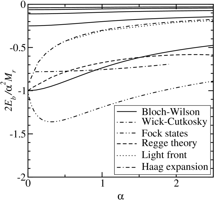
Figure 1: The spectrum of binding energies $E_{b}=E-m_{A}-m_{B}$ for $S$–states in the equal–mass case, compared to the ground state energies of the Wick-Cutkosky model [10], the Hamiltonian eigenvalue equation in a Fock space truncation [21], the Regge theory predictions [22], the light–front calculation [23], and the Haag expansion results [24] in their domain of validity.

It is a remarkable fact that the numerical curves for all other relativistic bound state equations presented in Fig. 1 do not show a quadratic behavior for small $\alpha$ (disregarding the results from the Haag expansion which does not have a proper nonrelativistic limit), which points to the existence of an order-$(m_{r}\alpha^{3})$ term in their expansion around the nonrelativistic limit. In fact, it is known that there appears a “curious” term of order $m_{r}\alpha^{3}\ln\alpha$ in the ladder approximation to the Bethe-Salpeter equation in such an expansion [11]. A simple power-counting argument cannot exclude the existence of contributions to the order $m_{r}\alpha^{3}$ (or $m_{r}\alpha^{3}\ln\alpha$) from the terms of order $H_{1}^{4}$ in the expansion of $H_{B}$ derived from the Dyson series (2) which are not considered in the present paper. However, from our experience with QED (e.g., the hydrogen atom and positronium) including terms of the order $H_{1}^{4}$, such contributions are certainly not expected. Note that a contribution of the next-higher order $m_{r}\alpha^{4}$ from the order-$H_{1}^{4}$ terms is necessary for the consistence of the results for $H_{B}$ and $H_{W}$ presented here which differ by a contribution of the order $m_{r}\alpha^{4}$, as we have seen (compare with the discussion at the end of Subsection 4.3). The definite solution of these issues, most importantly the question of whether the results presented here for the fine structure (from $H_{B}$) are complete, has to await the (complicated) evaluation of the $\mathcal{O}(H_{1}^{4})$ terms by the present or a different method.

To give a better idea of how the numerical results relate to the perturbative expansion around the nonrelativistic limit, we have plotted both in Fig. 2 for the ground state. The approximation by the perturbative expression is good only way below $\alpha=0.1$. We have also plotted the curve corresponding to all hermitian terms, i.e., omitting the contribution from Eq. (43$c$) in Eq. (83). Note that the latter curve lies closer to the numerical data points than the curve for the complete expressions, for intermediate values of $\alpha$.

Figure 2: The numerical results (diamonds) for the ground state binding energy, normalized as in Fig. 1, compared with the perturbative results (83) (solid line). We have also plotted the perturbative results without the contribution from the antihermitian term (dashed line).

5.2 Yukawa theory

For Yukawa theory, the calculation is technically, but not essentially, more complicated than for the Wick-Cutkosky model, due to the spin of the fermions. The necessary techniques for the evaluation of the relativistic corrections are presented in Appendix A. We will label the states by the standard spectroscopic notation $n{}^{\,2S+1\!}L_{J}$. The explicit results for principal qunatum numbers $n=1,2$ are, again term by term in the order they appear in the momentum expansion of the effective Hamiltonian, Eqs. (45$a$)–(45$e$),

$$\Delta E(1{}^{\,1\!}S_{0}) =\Delta E(1{}^{\,3\!}S_{1})=\left[-\frac{5}{8}\left(\frac{1}{m_{A}^{3}}+\frac{1}{m_{B}^{3}}\right)m_{r}^{3}+\frac{3}{4}\left(\frac{1}{m_{A}^{2}}+\frac{1}{m_{B}^{2}}\right)m_{r}^{2}\right.$$

$$\phantom{=}\hskip 85.35826pt\left.+\frac{1}{\pi^{2}}+\left(-\frac{1}{2}+\frac{1}{4}\right)\left(\frac{1}{m_{A}^{2}}+\frac{1}{m_{B}^{2}}\right)m_{r}^{2}\right]m_{r}\alpha^{4}\>,$$

$$\Delta E(2{}^{\,1\!}S_{0}) =\Delta E(2{}^{\,3\!}S_{1})=\left[-\frac{13}{128}\left(\frac{1}{m_{A}^{3}}+\frac{1}{m_{B}^{3}}\right)m_{r}^{3}+\frac{7}{64}\left(\frac{1}{m_{A}^{2}}+\frac{1}{m_{B}^{2}}\right)m_{r}^{2}\right.$$

$$\phantom{=}\hskip 85.35826pt\left.+\frac{1}{8\pi^{2}}+\left(-\frac{1}{16}+\frac{3}{64}\right)\left(\frac{1}{m_{A}^{2}}+\frac{1}{m_{B}^{2}}\right)m_{r}^{2}\right]m_{r}\alpha^{4}\>,$$

$$\Delta E(2{}^{\,3\!}P_{0}) =\left[-\frac{7}{384}\left(\frac{1}{m_{A}^{3}}+\frac{1}{m_{B}^{3}}\right)m_{r}^{3}+\frac{5}{192}\left(\frac{1}{m_{A}^{2}}+\frac{1}{m_{B}^{2}}\right)m_{r}^{2}\right.$$

$$\phantom{=}\hskip 85.35826pt\left.+\frac{1}{24\pi^{2}}+\left(-\frac{1}{48}+\frac{9}{192}\right)\left(\frac{1}{m_{A}^{2}}+\frac{1}{m_{B}^{2}}\right)m_{r}^{2}\right]m_{r}\alpha^{4}\>,$$

$$\Delta E^{\prime}(2{}^{\,3\!}P_{1}) =\left[-\frac{7}{384}\left(\frac{1}{m_{A}^{3}}+\frac{1}{m_{B}^{3}}\right)m_{r}^{3}+\frac{5}{192}\left(\frac{1}{m_{A}^{2}}+\frac{1}{m_{B}^{2}}\right)m_{r}^{2}\right.$$

$$\phantom{=}\hskip 85.35826pt\left.+\frac{1}{24\pi^{2}}+\left(-\frac{1}{48}+\frac{7}{192}\right)\left(\frac{1}{m_{A}^{2}}+\frac{1}{m_{B}^{2}}\right)m_{r}^{2}\right]m_{r}\alpha^{4}\>,$$

$$\Delta E^{\prime}(2{}^{\,1\!}P_{1}) =\left[-\frac{7}{384}\left(\frac{1}{m_{A}^{3}}+\frac{1}{m_{B}^{3}}\right)m_{r}^{3}+\frac{5}{192}\left(\frac{1}{m_{A}^{2}}+\frac{1}{m_{B}^{2}}\right)m_{r}^{2}\right.$$

$$\phantom{=}\hskip 85.35826pt\left.+\frac{1}{24\pi^{2}}+\left(-\frac{1}{48}+\frac{5}{192}\right)\left(\frac{1}{m_{A}^{2}}+\frac{1}{m_{B}^{2}}\right)m_{r}^{2}\right]m_{r}\alpha^{4}\>,$$

$$\Delta E(2{}^{\,3\!}P_{2}) =\left[-\frac{7}{384}\left(\frac{1}{m_{A}^{3}}+\frac{1}{m_{B}^{3}}\right)m_{r}^{3}+\frac{5}{192}\left(\frac{1}{m_{A}^{2}}+\frac{1}{m_{B}^{2}}\right)m_{r}^{2}\right.$$

$$\phantom{=}\hskip 85.35826pt\left.+\frac{1}{24\pi^{2}}+\left(-\frac{1}{48}+\frac{3}{192}\right)\left(\frac{1}{m_{A}^{2}}+\frac{1}{m_{B}^{2}}\right)m_{r}^{2}\right]m_{r}\alpha^{4}\>.$$ (84)

The results for the states $2{}^{\,3\!}P_{1}$ and $2{}^{\,1\!}P_{1}$ bear primes because these states (which are degenerate in the nonrelativistic limit) mix through the equal off-diagonal matrix elements

$$-\frac{\sqrt{2}}{96}\left(\frac{1}{m_{A}^{2}}-\frac{1}{m_{B}^{2}}\right)m_{r}^{3}\alpha^{4}\>.$$ (85)

To obtain the energy corrections properly, one hence has to diagonalize the corresponding $2\times 2$ matrix with diagonal elements $\Delta E^{\prime}(2{}^{\,3\!}P_{1})$ and $\Delta E^{\prime}(2{}^{\,1\!}P_{1})$. The explicit expressions for the eigenvalues are not too illuminating.

Compared to the results for the Wick-Cutkosky model, in the Yukawa case the contributions from the “nonlocal” term (43$b$) are reduced to half their value by a contribution from the normalization of the Dirac spinors in (45$b$), and a positive contribution from the spin structure enters. The fact that the “nonlocal” contribution is reduced leads to a sign change for the relativistic corrections of the $1S$ states depending on the mass ratio: in the case of equal masses, all corrections are positive, while the corrections for $1{}^{\,1\!}S_{0}$ and $1{}^{\,3\!}S_{1}$ turn negative in the one-body limit $m_{B}\to\infty$.

As for the “mixing” states $2{}^{\,3\!}P_{1}$ and $2{}^{\,1\!}P_{1}$, in the case of equal masses the off-diagonal elements (85) vanish, and $\Delta E^{\prime}(2{}^{\,3\!}P_{1})$ and $\Delta E^{\prime}(2{}^{\,1\!}P_{1})$ directly give the energy corrections of the states. Observe the equal spacing between the energy corrections of the four $2P$ states in this case which is nicely reproduced by the numerical results up to intermediate coupling constants. In the one-body limit, on the other hand, the states mix strongly, and one of the eigenstates becomes degenerate with the state $2{}^{\,3\!}P_{0}$, the other with $2{}^{\,3\!}P_{2}$. These degeneracies and the ones of $1{}^{\,1\!}S_{0}$ with $1{}^{\,3\!}S_{1}$ and of $2{}^{\,1\!}S_{0}$ with $2{}^{\,3\!}S_{1}$, are exact in the one-body limit, for any value of the coupling constant. The reason for these twofold degeneracies is that the spin of fermion $B$ decouples from the dynamics in the limit $m_{B}\to\infty$. In fact, the states $2{}^{\,3\!}P_{0}$ and the mixture of $2{}^{\,3\!}P_{1}$ and $2{}^{\,1\!}P_{1}$ degenerate with the former, are eigenstates of the total angular momentum (relative orbital angular momentum and spin) of fermion $A$ with eigenvalue $j_{A}=1/2$, while state $2{}^{\,3\!}P_{2}$ and the other linear combination of $2{}^{\,3\!}P_{1}$ and $2{}^{\,1\!}P_{1}$ are $j_{A}$ eigenstates with eigenvalue 3/2. Note that the $j_{A}=1/2$ state lies higher in energy than the $j_{A}=3/2$ state.

Close to the one-body limit, we can check for hyperfine structure by expanding the expressions for the energy corrections of the $2P$ states in Eq. (84) and the off-diagonal elements (85) in powers of $m_{A}/m_{B}$. Obviously, there is no hyperfine splitting for the $1S$ and the $2S$ states to any order in $m_{A}/m_{B}$ (and to order $m_{r}\alpha^{4}$). After diagonalizing the submatrix for the states $2{}^{\,3\!}P_{1}$ and $2{}^{\,1\!}P_{1}$, one finds no hyperfine splitting to the order $m_{A}/m_{B}$, while there does appear such a splitting to the next order, $(m_{A}/m_{B})^{2}$. These results on the hyperfine structure have been anticipated in Ref. [3].

The perturbative results (84) show all the qualitative features that we have found in the numerical solutions of the effective Schrödinger equation (20) in Ref. [3]. In quantitative terms, the agreement between numerical and perturbative analytical results is similar to the case of the Wick-Cutkosky model (see Fig. 2) for the $S$ states, and somewhat better for the $P$ states. Just like in Fig. 2, the perturbative curve without the contribution of the antihermitian term lies closer to the numerical results for intermediate coupling constants than the full perturbative curve. It appears that the antihermitian term is only important for very small $\alpha$ and does practically not contribute for larger values of $\alpha$. The most clear-cut case is the one of $\Delta E(2{}^{\,1\!}S_{0})$ = $\Delta E(2{}^{\,3\!}S_{1})$ in the one-body limit where the complete perturbative correction is positive, while its hermitian part is negative. In this case, the numerical values for very small $\alpha$ increase with the coupling constant as expected from the perturbative results, but then start to decrease and become negative roughly at $\alpha=0.35$, loosely following the “hermitian” curve for larger $\alpha$.

The peculiar role that is played by the contributions from the antihermitian term might lead one to the believe that these contributions are spurious and may cancel with other contributions from terms of the order $H_{1}^{4}$ in the expansion of the effective Hamiltonian. In this sense, the Okubo Hamiltonian $H_{W}$ would be a better choice for an effective Hamiltonian, because it simply does not contain the antihermitian term. However, the results of Appendix B suggest that, quite to the contrary, the terms of the order $H_{1}^{4}$ in the expansion of $H_{W}$ generate the hermitian equivalent of the term in question.

5.3 Quantum electrodynamics

Finally, we will present our results for QED in the Coulomb gauge, i.e., the expanded effective Hamiltonian of Eqs. (47$a$)-(47$f$). The explicit expressions are [25], term by term,

$$\Delta E(1{}^{\,1\!}S_{0}) =\bigg{[}-\frac{5}{8}\left(\frac{1}{m_{A}^{3}}+\frac{1}{m_{B}^{3}}\right)m_{r}^{3}+\left(\frac{3}{4}-\frac{1}{4}\right)\left(\frac{1}{m_{A}^{2}}+\frac{1}{m_{B}^{2}}\right)m_{r}^{2}$$

$$\phantom{=}\hskip 142.26378pt+\big{(}-2-1+0\big{)}\frac{m_{r}^{2}}{m_{A}m_{B}}\bigg{]}m_{r}\alpha^{4}\>,$$

$$\Delta E(1{}^{\,3\!}S_{1}) =\left[-\frac{5}{8}\left(\frac{1}{m_{A}^{3}}+\frac{1}{m_{B}^{3}}\right)m_{r}^{3}+\left(\frac{3}{4}-\frac{1}{4}\right)\left(\frac{1}{m_{A}^{2}}+\frac{1}{m_{B}^{2}}\right)m_{r}^{2}\right.$$

$$\phantom{=}\hskip 142.26378pt\left.+\left(\frac{2}{3}-1+0\right)\frac{m_{r}^{2}}{m_{A}m_{B}}\right]m_{r}\alpha^{4}\>,$$

$$\Delta E(2{}^{\,1\!}S_{0}) =\left[-\frac{13}{128}\left(\frac{1}{m_{A}^{3}}+\frac{1}{m_{B}^{3}}\right)m_{r}^{3}+\left(\frac{7}{64}-\frac{3}{64}\right)\left(\frac{1}{m_{A}^{2}}+\frac{1}{m_{B}^{2}}\right)m_{r}^{2}\right.$$

$$\phantom{=}\hskip 142.26378pt\left.+\left(-\frac{1}{4}-\frac{3}{16}+0\right)\frac{m_{r}^{2}}{m_{A}m_{B}}\right]m_{r}\alpha^{4}\>,$$

$$\Delta E(2{}^{\,3\!}S_{1}) =\left[-\frac{13}{128}\left(\frac{1}{m_{A}^{3}}+\frac{1}{m_{B}^{3}}\right)m_{r}^{3}+\left(\frac{7}{64}-\frac{3}{64}\right)\left(\frac{1}{m_{A}^{2}}+\frac{1}{m_{B}^{2}}\right)m_{r}^{2}\right.$$

$$\phantom{=}\hskip 142.26378pt\left.+\left(\frac{1}{12}-\frac{3}{16}+0\right)\frac{m_{r}^{2}}{m_{A}m_{B}}\right]m_{r}\alpha^{4}\>,$$

$$\Delta E(2{}^{\,3\!}P_{0}) =\left[-\frac{7}{384}\left(\frac{1}{m_{A}^{3}}+\frac{1}{m_{B}^{3}}\right)m_{r}^{3}+\left(\frac{5}{192}-\frac{3}{64}\right)\left(\frac{1}{m_{A}^{2}}+\frac{1}{m_{B}^{2}}\right)m_{r}^{2}\right.$$

$$\phantom{=}\hskip 142.26378pt\left.+\left(-\frac{1}{24}-\frac{3}{16}+\frac{1}{24}\right)\frac{m_{r}^{2}}{m_{A}m_{B}}\right]m_{r}\alpha^{4}\>,$$

$$\Delta E^{\prime}(2{}^{\,3\!}P_{1}) =\left[-\frac{7}{384}\left(\frac{1}{m_{A}^{3}}+\frac{1}{m_{B}^{3}}\right)m_{r}^{3}+\left(\frac{5}{192}-\frac{7}{192}\right)\left(\frac{1}{m_{A}^{2}}+\frac{1}{m_{B}^{2}}\right)m_{r}^{2}\right.$$

$$\phantom{=}\hskip 142.26378pt\left.+\left(\frac{1}{48}-\frac{7}{48}+\frac{1}{24}\right)\frac{m_{r}^{2}}{m_{A}m_{B}}\right]m_{r}\alpha^{4}\>,$$

$$\Delta E^{\prime}(2{}^{\,1\!}P_{1}) =\left[-\frac{7}{384}\left(\frac{1}{m_{A}^{3}}+\frac{1}{m_{B}^{3}}\right)m_{r}^{3}+\left(\frac{5}{192}-\frac{5}{192}\right)\left(\frac{1}{m_{A}^{2}}+\frac{1}{m_{B}^{2}}\right)m_{r}^{2}\right.$$

$$\phantom{=}\hskip 142.26378pt\left.+\left(0-\frac{5}{48}+\frac{1}{24}\right)\frac{m_{r}^{2}}{m_{A}m_{B}}\right]m_{r}\alpha^{4}\>,$$

$$\Delta E(2{}^{\,3\!}P_{2}) =\left[-\frac{7}{384}\left(\frac{1}{m_{A}^{3}}+\frac{1}{m_{B}^{3}}\right)m_{r}^{3}+\left(\frac{5}{192}-\frac{1}{64}\right)\left(\frac{1}{m_{A}^{2}}+\frac{1}{m_{B}^{2}}\right)m_{r}^{2}\right.$$

$$\phantom{=}\hskip 142.26378pt\left.+\left(-\frac{1}{240}-\frac{1}{16}+\frac{1}{24}\right)\frac{m_{r}^{2}}{m_{A}m_{B}}\right]m_{r}\alpha^{4}\>.$$ (86)

As in the case of Yukawa theory, the states $2{}^{\,3\!}P_{1}$ and $2{}^{\,1\!}P_{1}$ mix through the equal off-diagonal matrix elements

$$\frac{\sqrt{2}}{96}\left(\frac{1}{m_{A}^{2}}-\frac{1}{m_{B}^{2}}\right)m_{r}^{3}\alpha^{4}\>.$$ (87)

When we compare these results with Eq. (84) for Yukawa theory, the differences are the opposite sign of the “spin-orbit” term [Eq. (45$e$) vs. Eq. (47$c$)], the absence of retardation, and, of course, the terms (47$d$)–(47$f$) which introduce the hyperfine structure. The difference in signs of the spin-orbit terms changes the qualitative features of the spectrum drastically: nearly all energy corrections are negative, only $\Delta E(1{}^{\,3\!}S_{1})$ becomes positive for mass ratios $m_{A}/m_{B}$ close to one. The level ordering of the $2P$ states is just opposite to the Yukawa case. In the one-body limit, the characteristic degeneracies appear, but in addition the $2S$ states become degenerate with the $2P$ states with $j_{A}=1/2$ (compare with the discussion of the one-body limit in the previous subsection). This is, of course, just the famous degeneracy in orbital angular momentum characteristic of the Coulomb potential (note that this degeneracy is broken in Yukawa theory by the retardation terms). Also, the $2P$ states with $j_{A}=1/2$ have a lower energy in QED than the $j_{A}=3/2$ states.

The hyperfine structure terms split the energies of the $1S$ and the $2S$ states. Close to the one-body limit, we can again expand the expressions (86) in powers of $m_{A}/m_{B}$ to obtain the hyperfine splittings (after diagonalizing the $2\times 2$ matrix for the states $2{}^{\,3\!}P_{1}$ and $2{}^{\,1\!}P_{1}$), which now appear to the order $m_{A}/m_{B}$ (and $m_{r}\alpha^{4}$). Our results (86) coincide completely with the ones in Ref. [5] close to the one-body limit and for the case of equal masses [25] (in the latter case, they coincide with the positronium results omitting the contributions from virtual annihilation there). In fact, one can show that the expanded effective Schrödinger equation in Eqs. (47$a$)–(47$f$) is identical to the Pauli approximation of the Breit equation (and in the one-body limit to the Pauli approximation of the Dirac equation) [5]. Depending on the form in which the latter equations are written, the identification of terms may require some algebraic labor. In particular, the Pauli approximation of the Breit and Dirac equations are sometimes given in a not manifestly hermitian form. In any case, the identity of the equations implies the identity of the lowest-order relativistic corrections, for any state and any mass ratio. We conclude that our approach reproduces the lowest-order fine and hyperfine structure completely (at least) in the case of QED, from the effective Hamiltonian ($H_{B}$ or $H_{W}$) to order $H_{1}^{2}$, and it does so in a very transparent and economic way.

To sum up, we have argued in this paper that we can obtain the lowest-order fine and hyperfine structure in nearly nonrelativistic bound systems in a very straightforward way from the application of the generalized Gell-Mann–Low theorem. We have verified this claim for bound states in QED, and we have presented, for the first time to our knowledge, results for the fine and hyperfine structure of bound states in the Wick-Cutkosky model and Yukawa theory. Although the results are physically appealing, we have as yet no proof that our calculation of the fine and hyperfine structure in the latter theories is complete. We have emphasized the contributions from the retardation in the effective potential for the Wick-Cutkosky model and Yukawa theory, and discussed the role of a peculiar antihermitian term that appears in this context, in particular with respect to two possible choices $H_{B}$ and $H_{W}$ for the effective Hamiltonian.

Acknowledgments

The author is grateful to Norbert E. Ligterink for many interesting discussions on the subject and for help with the graphics. Financial support by CIC-UMSNH and Conacyt project 32729-E is acknowledged.

Appendix A A collection of useful formulae

We will present in this appendix the formulae that are used in the actual analytic calculations of the perturbative corrections to the Coulomb energy eigenvalues. Since we have done all of the calculations directly in momentum space (as a warm-up for more complex calculations in the future), we need, first of all, the Coulomb wave functions $\phi_{nlm}(\mathbf{p})$ in momentum space, here for the principal quantum numbers $n=1,2$:

$$\phi_{100}(\mathbf{p}) =\frac{16\pi\,(m_{r}\alpha)^{5/2}}{\left[(m_{r}\alpha)^{2}+p^{2}\right]^{2}}\,Y_{00}(\hat{\mathbf{p}})$$

$$\phi_{200}(\mathbf{p}) =\frac{\displaystyle 4\pi\sqrt{2}\,(m_{r}\alpha)^{5/2}\left(p^{2}-\frac{(m_{r}\alpha)^{2}}{4}\right)}{\displaystyle\left(\frac{(m_{r}\alpha)^{2}}{4}+p^{2}\right)^{3}}\,Y_{00}(\hat{\mathbf{p}})$$

$$\phi_{21m}(\mathbf{p}) =\frac{\displaystyle 4\pi\sqrt{\frac{2}{3}}\,(m_{r}\alpha)^{7/2}p}{\displaystyle\left(\frac{(m_{r}\alpha)^{2}}{4}+p^{2}\right)^{3}}\,Y_{1m}(\hat{\mathbf{p}})\>.$$ (88)

The wave functions are normalized to

$$\int\frac{d^{3}p}{(2\pi)^{3}}\,\lvert\phi_{nlm}(\mathbf{p})\rvert^{2}=1\>.$$ (89)

In the cases of Yukawa theory and QED, the expressions above still have to be multiplied with the appropriate Pauli spinors for the spin orientation of the fermions. It is convenient in the latter cases to use total angular momentum eigenstates. In order to make contact to the usual spectroscopy, we first couple the two spins 1/2 to a total spin $S=0,1$, and then couple the total spin with the relative orbital angular momentum $l$ to the total angular momentum $J,M$. The explicit results for the total angular momentum eigenstates ${}^{\,2S+1\!}\mathcal{Y}_{lM}^{J}(\hat{\mathbf{p}})$ are [3], in terms of the well-known eigenstates $\chi_{S,m_{S}}$ of total spin:

$${}^{\,1\!}\mathcal{Y}_{JM}^{J}(\hat{\mathbf{p}}) =Y_{JM}(\hat{\mathbf{p}})\,\chi_{00}\>,$$

$${}^{\,3\!}\mathcal{Y}_{J-1,M}^{J}(\hat{\mathbf{p}}) =\frac{1}{\sqrt{2J(2J-1)}}\left[\sqrt{(J-M-1)(J-M)}\,Y_{J-1,M+1}(\hat{\mathbf{p}})\,\chi_{1,-1}\right.$$

$$\phantom{=}+\sqrt{2(J-M)(J+M)}\,Y_{J-1,M}(\hat{\mathbf{p}})\,\chi_{10}$$

$$\phantom{=}\left.+\sqrt{(J+M-1)(J+M)}\,Y_{J-1,M-1}(\hat{\mathbf{p}})\,\chi_{11}\right]\quad(J\geq 1)\>,$$

$${}^{\,3\!}\mathcal{Y}_{JM}^{J}(\hat{\mathbf{p}}) =\frac{1}{\sqrt{2J(J+1)}}\left[\sqrt{(J-M)(J+M+1)}\,Y_{J,M+1}(\hat{\mathbf{p}})\,\chi_{1,-1}\right.$$

$$\phantom{=}\left.+\sqrt{2}\,M\,Y_{JM}(\hat{\mathbf{p}})\,\chi_{10}-\sqrt{(J-M+1)(J+M)}\,Y_{J,M-1}(\hat{\mathbf{p}})\,\chi_{11}\right]\quad(J\geq 1)\>,$$

$${}^{\,3\!}\mathcal{Y}_{J+1,M}^{J}(\hat{\mathbf{p}}) =\frac{1}{\sqrt{2(J+1)(2J+3)}}\left[\sqrt{(J+M+1)(J+M+2)}\,Y_{J+1,M+1}(\hat{\mathbf{p}})\,\chi_{1,-1}\right.$$

$$\phantom{=}-\sqrt{2(J-M+1)(J+M+1)}\,Y_{J+1,M}(\hat{\mathbf{p}})\,\chi_{10}$$

$$\phantom{=}\left.+\sqrt{(J-M+1)(J-M+2)}\,Y_{J+1,M-1}(\hat{\mathbf{p}})\,\chi_{11}\right]\>.$$ (90)

For the calculation of the perturbative corrections in these theories, one needs to apply the operators $(\mathbf{p}\cdot\bm{\sigma}_{A,B})$ to these total angular momentum eigenstates. The corresponding formulae were also worked out in Ref. [3]. They read

$$(\mathbf{p}\cdot\bm{\sigma}_{A})\,{}^{\,1\!}\mathcal{Y}_{JM}^{J}(\hat{\mathbf{p}}) =p\left(\sqrt{\frac{J}{2J+1}}\,{}^{\,3\!}\mathcal{Y}_{J-1,M}^{J}(\hat{\mathbf{p}})-\sqrt{\frac{J+1}{2J+1}}\,{}^{\,3\!}\mathcal{Y}_{J+1,M}^{J}(\hat{\mathbf{p}})\right)\>,$$

$$(\mathbf{p}\cdot\bm{\sigma}_{A})\,{}^{\,3\!}\mathcal{Y}_{J-1,M}^{J}(\hat{\mathbf{p}}) =p\left(\sqrt{\frac{J}{2J+1}}\,{}^{\,1\!}\mathcal{Y}_{JM}^{J}(\hat{\mathbf{p}})-\sqrt{\frac{J+1}{2J+1}}\,{}^{\,3\!}\mathcal{Y}_{JM}^{J}(\hat{\mathbf{p}})\right)\>,$$

$$(\mathbf{p}\cdot\bm{\sigma}_{A})\,{}^{\,3\!}\mathcal{Y}_{JM}^{J}(\hat{\mathbf{p}}) =-p\left(\sqrt{\frac{J+1}{2J+1}}\,{}^{\,3\!}\mathcal{Y}_{J-1,M}^{J}(\hat{\mathbf{p}})+\sqrt{\frac{J}{2J+1}}\,{}^{\,3\!}\mathcal{Y}_{J+1,M}^{J}(\hat{\mathbf{p}})\right)\>,$$

$$(\mathbf{p}\cdot\bm{\sigma}_{A})\,{}^{\,3\!}\mathcal{Y}_{J+1,M}^{J}(\hat{\mathbf{p}}) =-p\left(\sqrt{\frac{J+1}{2J+1}}\,{}^{\,1\!}\mathcal{Y}_{JM}^{J}(\hat{\mathbf{p}})+\sqrt{\frac{J}{2J+1}}\,{}^{\,3\!}\mathcal{Y}_{JM}^{J}(\hat{\mathbf{p}})\right)\>,$$ (91)

and

$$(\mathbf{p}\cdot\bm{\sigma}_{B})\,{}^{\,1\!}\mathcal{Y}_{JM}^{J}(\hat{\mathbf{p}}) =-p\left(\sqrt{\frac{J}{2J+1}}\,{}^{\,3\!}\mathcal{Y}_{J-1,M}^{J}(\hat{\mathbf{p}})-\sqrt{\frac{J+1}{2J+1}}\,{}^{\,3\!}\mathcal{Y}_{J+1,M}^{J}(\hat{\mathbf{p}})\right)\>,$$

$$(\mathbf{p}\cdot\bm{\sigma}_{B})\,{}^{\,3\!}\mathcal{Y}_{J-1,M}^{J}(\hat{\mathbf{p}}) =-p\left(\sqrt{\frac{J}{2J+1}}\,{}^{\,1\!}\mathcal{Y}_{JM}^{J}(\hat{\mathbf{p}})+\sqrt{\frac{J+1}{2J+1}}\,{}^{\,3\!}\mathcal{Y}_{JM}^{J}(\hat{\mathbf{p}})\right)\>,$$

$$(\mathbf{p}\cdot\bm{\sigma}_{B})\,{}^{\,3\!}\mathcal{Y}_{JM}^{J}(\hat{\mathbf{p}}) =-p\left(\sqrt{\frac{J+1}{2J+1}}\,{}^{\,3\!}\mathcal{Y}_{J-1,M}^{J}(\hat{\mathbf{p}})+\sqrt{\frac{J}{2J+1}}\,{}^{\,3\!}\mathcal{Y}_{J+1,M}^{J}(\hat{\mathbf{p}})\right)\>,$$

$$(\mathbf{p}\cdot\bm{\sigma}_{B})\,{}^{\,3\!}\mathcal{Y}_{J+1,M}^{J}(\hat{\mathbf{p}}) =p\left(\sqrt{\frac{J+1}{2J+1}}\,{}^{\,1\!}\mathcal{Y}_{JM}^{J}(\hat{\mathbf{p}})-\sqrt{\frac{J}{2J+1}}\,{}^{\,3\!}\mathcal{Y}_{JM}^{J}(\hat{\mathbf{p}})\right)\>.$$ (92)

In the special case $J=0$, the states ${}^{\,3\!}\mathcal{Y}_{J-1,M}^{J}(\hat{\mathbf{p}})$ and ${}^{\,3\!}\mathcal{Y}_{JM}^{J}(\hat{\mathbf{p}})$ do not exist, and on the right-hand sides for the application of one of the helicity operators to ${}^{\,1\!}\mathcal{Y}_{JM}^{J}(\hat{\mathbf{p}})$ and ${}^{\,3\!}\mathcal{Y}_{J+1,M}^{J}(\hat{\mathbf{p}})$, only one term remains. For the application of $(\bm{\sigma}_{A}\cdot\bm{\sigma}_{B})$, we use the well-known identity

$$(\bm{\sigma}_{A}\cdot\bm{\sigma}_{B}){}^{\,2S+1\!}\mathcal{Y}_{lM}^{J}(\hat{\mathbf{p}})=\left[2S(S+1)-3\right]{}^{\,2S+1\!}\mathcal{Y}_{lM}^{J}(\hat{\mathbf{p}})\>.$$ (93)

After the application of these formulae, the angular integrations can be performed with the help of the partial wave decomposition and the spherical harmonics addition theorem, Eq. (52). To this end, the coefficient functions have to be calculated from Eq. (53) which is elementary in all relevant cases.

Finally, the integrations over $p$ and $p^{\prime}$ have to be performed. All appearing integrals are again elementary, the only exception being integrals of the type

$$\int_{0}^{\infty}dp\,\frac{p^{2k+1}}{(\lambda^{2}+p^{2})^{n+1}}\ln\left(\frac{p+p^{\prime}}{|p-p^{\prime}|}\right)\>,$$ (94)

with $n=1,2,3,\ldots$ and $0\leq k\leq n$. All these integrals can be obtained by differentiation with respect to $\lambda^{2}$ and trivial algebraic manipulations of the fraction from

$$I=\int_{0}^{\infty}dp\,\frac{p}{\lambda^{2}+p^{2}}\ln\left(\frac{p+p^{\prime}}{|p-p^{\prime}|}\right)\>,$$ (95)

which we will now evaluate. To this end, consider the analytic function

$$F(p)=\frac{p}{\lambda^{2}+p^{2}}\ln\left(\frac{p+p^{\prime}}{p-p^{\prime}}\right)$$ (96)

which is even under $p\to-p$ and its real part coincides with the integrand of $I$, so that

$$I=\frac{1}{2}\,\text{Re}\int_{-\infty}^{\infty}dp\,F(p)\>.$$ (97)

As far as its analytic structure is concerned, $F(p)$ has simple poles at $p=\pm i\lambda$ and a cut on the real axis from $-p^{\prime}$ to $p^{\prime}$. We can hence evaluate $I$ by integrating along the real axis and (e.g.) the upper rim of the cut and closing the contour through the upper infinite semicircle. Then only the pole at $i\lambda$ is picked up (suppose $\lambda>0$), and the result is

$$I=\pi\arctan(p^{\prime}/\lambda)\>.$$ (98)

Appendix B A transformation of Foldy-Wouthuysen type

In this appendix we will devise an alternative method for the calculation of the contributions to the energy corrections that arise from the antihermitian term (43$c$) or (45$c$) in the Wick-Cutkosky model or Yukawa theory, respectively. Unlike the “direct” calculation in Section 4.3, we will construct a similarity transformation that converts $H_{B}$ to a hermitian operator, to the perturbative order required. Since the eigenvalues are unchanged under the similarity transformation, we can then use common “hermitian” perturbation theory to calculate the corrections to the energy.

In fact, in Section 3 a similarity transformation was introduced that does just this, see Eq. (30). Although we will take the form of this transformation as a motivation, the transformation (30) as it stands is plagued by infrared divergencies. For this reason we rather choose a transformation of the Foldy-Wouthuysen type because in this case the Baker-Campell-Hausdorff formula guarantees a convenient commutator structure for the transformed operator. Since the similarity transform has to map a nonhermitian operator to a hermitian one (at least to a certain perturbative order), it can obviously not be unitary. We hence consider transformations of the general form

$$S=\exp\left(-T^{\scriptscriptstyle(1)}-T^{\scriptscriptstyle(2)}-\ldots\right):\Omega_{0}\to\Omega_{0}\>,$$ (99)

where the operator $T^{\scriptscriptstyle(2)}$ is of higher perturbative order than $T^{\scriptscriptstyle(1)}$, etc. It follows for the similarity transformed Hamiltonian

$$H_{B}^{\prime}=S^{-1}H_{B}S=H_{B}+\left[T^{\scriptscriptstyle(1)},H_{B}\right]+\frac{1}{2}\big{[}T^{\scriptscriptstyle(1)},\left[T^{\scriptscriptstyle(1)},H_{B}\right]\big{]}+\left[T^{\scriptscriptstyle(2)},H_{B}\right]+\ldots\>.$$ (100)

We could now take the similarity transformation to coincide with the one in Eq. (30) to lowest nontrivial order in $g$,

$$S^{\prime}=(U_{B}^{\dagger}U_{B})^{-1/2}+\mathcal{O}(g^{4})\>,$$ (101)

by choosing

$$T^{\prime\scriptscriptstyle(1)}=\frac{1}{2}\int_{-\infty}^{0}dt_{1}\int_{-\infty}^{0}dt_{2}\,e^{-\epsilon(\lvert t_{1}\rvert+\lvert t_{2}\rvert)}P_{0}H_{1}(t_{1})H_{1}(t_{2})P_{0}$$ (102)

[cf. Eq. (32)]. However, this is still a quite complicated choice because of the infrared divergencies mentioned before, so we will take a somewhat simpler alternative and leave the diagonal contributions (vacuum and kinetic energies) out of $T^{\prime\scriptscriptstyle(1)}$, defining $T^{\scriptscriptstyle(1)}$ explicitly through its matrix elements in the center-of-mass system as

$$\langle\mathbf{p},r,s|T^{\scriptscriptstyle(1)}|\mathbf{p}^{\prime},r^{\prime},s^{\prime}\rangle$$

$$=-\frac{g^{2}}{2\sqrt{2E_{\mathbf{p}}^{A}\,2E_{\mathbf{p}}^{B}\,2E_{\mathbf{p}^{\prime}}^{A}\,2E_{\mathbf{p}^{\prime}}^{B}}}\,\frac{\left[\bar{u}_{A}(\mathbf{p},r)\,u_{A}(\mathbf{p}^{\prime},r^{\prime})\right]\left[\bar{u}_{B}(-\mathbf{p},s)\,u_{B}(-\mathbf{p}^{\prime},s^{\prime})\right]}{E_{\mathbf{p}}^{A}+E_{\mathbf{p}}^{B}-E_{\mathbf{p}^{\prime}}^{A}-E_{\mathbf{p}^{\prime}}^{B}}$$

$$\phantom{=}\times\frac{1}{2\sqrt{(\mathbf{p}-\mathbf{p}^{\prime})^{2}+\mu^{2}}}\left(\frac{1}{E_{\mathbf{p}}^{A}+\sqrt{(\mathbf{p}-\mathbf{p}^{\prime})^{2}+\mu^{2}}-E_{\mathbf{p}^{\prime}}^{A}}+\frac{1}{E_{\mathbf{p}}^{B}+\sqrt{(\mathbf{p}-\mathbf{p}^{\prime})^{2}+\mu^{2}}-E_{\mathbf{p}^{\prime}}^{B}}\right.$$

$$\phantom{=}\hskip 28.45274pt\left.-\frac{1}{E_{\mathbf{p}^{\prime}}^{A}+\sqrt{(\mathbf{p}-\mathbf{p}^{\prime})^{2}+\mu^{2}}-E_{\mathbf{p}}^{A}}-\frac{1}{E_{\mathbf{p}^{\prime}}^{B}+\sqrt{(\mathbf{p}-\mathbf{p}^{\prime})^{2}+\mu^{2}}-E_{\mathbf{p}}^{B}}\right)$$ (103)

Definition (103) properly applies to Yukawa theory, for the Wick-Cutkosky model one just has to omit the products of Dirac spinors. We have introduced a mass $\mu$ for the exchanged boson as an IR regulator (see below).

Equation (100) above, to lowest nontrivial order, then leads to

$$H_{B}^{\prime}=H_{B}+\left[T^{\scriptscriptstyle(1)},H_{0}\right]+\mathcal{O}(g^{4})=H_{W}+\mathcal{O}(g^{4})\>,$$ (104)

just as for the full transformation in Eq. (33). However, while we were content in Section 3 with calculating $H_{W}$ strictly to order $H_{1}^{2}$, for the lowest-order fine and hyperfine structure we need all terms of order $m_{r}\alpha^{4}$, and such terms may arise from the order-$g^{4}$ contibutions to $H_{B}^{\prime}$. In fact, we will now show that this is the case, which means that $H_{B}^{\prime}\neq H_{W}$ to the order $m_{r}\alpha^{4}$.

In order to extract the terms of order $m_{r}\alpha^{4}$ from the order-$g^{4}$ terms in Eq. (100), it is sufficient to work with $T^{\scriptscriptstyle(1)}$ to lowest order in a momentum expansion, explicitly

$$\langle\mathbf{p},r,s|T^{\scriptscriptstyle(1)}|\mathbf{p}^{\prime},r^{\prime},s^{\prime}\rangle=\frac{2\pi\alpha}{\left[(\mathbf{p}-\mathbf{p}^{\prime})^{2}+\mu^{2}\right]^{3/2}}\,\delta_{rr^{\prime}}\delta_{ss^{\prime}}+\mathcal{O}(\alpha^{3})$$ (105)

(for Yukawa theory, for the Wick-Cutkosky model just omit the Kronecker deltas). For the discussion of IR convergence or divergence, as well as for the estimation of the order in $\alpha$ by IR power counting, we have to take into account that Eq. (105) is integrated over $d^{3}p^{\prime}$ when it is applied to a function of $\mathbf{p}^{\prime}$. This adds three powers of $\alpha$ to the power counting, so that the leading term in Eq. (105) is IR divergent and of order $\alpha$ (the IR regulator is ignored in the power counting). The fact that $T^{\scriptscriptstyle(1)}$ is IR divergent to lowest order is uncomfortable. Incidentally, given the relation of $T^{\scriptscriptstyle(1)}$ to $(U_{B}^{\dagger}U_{B})^{-1/2}$ and hence to $U_{W}$, this IR divergence sheds doubts on the proper existence of the Okubo map. We have not completely analyzed the question of the IR convergence or divergence of $U_{W}$ yet. In any event, the transformed Hamiltonian will turn out to be IR convergent to the order $m_{r}\alpha^{4}$ considered at present.

Now consider the momentum expansion of

$$\langle\mathbf{p},r,s|H_{B}+\frac{1}{2}\left[T^{\scriptscriptstyle(1)},H_{0}\right]|\mathbf{p}^{\prime},r^{\prime},s^{\prime}\rangle$$

$$=\langle\mathbf{p},r,s|H_{0}|\mathbf{p}^{\prime},r^{\prime},s^{\prime}\rangle-\frac{4\pi\alpha}{(\mathbf{p}-\mathbf{p}^{\prime})^{2}+\mu^{2}}\left(1-\frac{1}{8m_{r}}\frac{p^{2}-p^{\prime 2}}{\sqrt{(\mathbf{p}-\mathbf{p}^{\prime})^{2}+\mu^{2}}}\right)\delta_{rr^{\prime}}\delta_{ss^{\prime}}+\mathcal{O}(m_{r}\alpha^{4})$$ (106)

(again omitting the Kronecker deltas for the case of the Wick-Cutkosky model). Observe that all the terms are IR convergent by power counting, hence the IR cutoff $\mu$ is not stictly necessary here. When the commutator with $T^{\scriptscriptstyle(1)}$ is taken in Eq. (100), the term with $H_{0}$ on the right-hand-side of Eq. (106) contributes to $H_{W}$ in Eq. (104), the following term of order $m_{r}\alpha^{2}$ does not contribute at all up to orders $m_{r}\alpha^{4}$, and it is the last term of order $m_{r}\alpha^{3}$ which gives the important order-$m_{r}\alpha^{4}$ contribution with matrix elements

$$-\frac{2\pi^{2}\alpha^{2}}{m_{r}}\int\frac{d^{3}q}{(2\pi)^{3}}\frac{(\mathbf{p}-\mathbf{q})\cdot(\mathbf{q}-\mathbf{p}^{\prime})}{\left[(\mathbf{p}-\mathbf{q})^{2}+\mu^{2}\right]^{3/2}\left[(\mathbf{q}-\mathbf{p}^{\prime})^{2}+\mu^{2}\right]^{3/2}}\,\delta_{rr^{\prime}}\delta_{ss^{\prime}}\>.$$ (107)

The latter expression is IR finite by power counting, hence the limit $\mu\to 0$ can safely be taken. It is then simple to perform the $d^{3}q$-integration, with the final result

$$\langle\mathbf{p},r,s|H_{B}^{\prime}|\mathbf{p}^{\prime},r^{\prime},s^{\prime}\rangle=\langle\mathbf{p},r,s|H_{W}|\mathbf{p}^{\prime},r^{\prime},s^{\prime}\rangle+\frac{\alpha^{2}}{m_{r}}\frac{1}{\lvert\mathbf{p}-\mathbf{p}^{\prime}\rvert}\,\delta_{rr^{\prime}}\delta_{ss^{\prime}}+\mathcal{O}(m_{r}\alpha^{5})$$ (108)

(without the Kronecker deltas for the Wick-Cutkosky model, as usual). This result coincides with the calculation in second-order “antihermitian” perturbation theory, see Eq. (82). The possible physical significance of the “new” $m_{r}\alpha^{4}$-term is discussed at the end of Subsection 4.3. It appears plausible from the result (108) and the consistency of the general formalism that this additional term is also generated by the similarity transformation $(U_{B}^{\dagger}U_{B})^{-1/2}$.

To close this appendix, let us have a look at the contributions to order $m_{r}\alpha^{5}$ in $H_{B}^{\prime}$. It is out of the question to present any details of the corresponding lengthy calculations, hence we will be content here with quoting the main results. First of all, it can be shown that all contributions of this order come from the next-higher terms in the expansions (105) and (106), inserted in the commutator

$$\left[T^{\scriptscriptstyle(1)},H_{B}+\frac{1}{2}\left[T^{\scriptscriptstyle(1)},H_{0}\right]\right]\>.$$ (109)

The complete result is cumbersome, but we will concentrate here on the IR divergent contributions that potentially invalidate the similarity transformation. They are explicitly given by the antihermitian expression

$$\langle\mathbf{p},r,s|H_{B}^{\prime}|\mathbf{p}^{\prime},r^{\prime},s^{\prime}\rangle\sim\frac{4\pi^{2}\alpha^{2}}{3m_{r}^{2}}\int\frac{d^{3}q}{(2\pi)^{3}}\frac{p^{2}-p^{\prime 2}}{\left[(\mathbf{p}-\mathbf{q})^{2}+\mu^{2}\right]^{3/2}\left[(\mathbf{q}-\mathbf{p}^{\prime})^{2}+\mu^{2}\right]}\,\delta_{rr^{\prime}}\delta_{ss^{\prime}}+\mathcal{O}(m_{r}\alpha^{6})\>,$$ (110)

where “$\sim$” refers to the equality of the IR divergent terms. It is now possible to remove these terms from $H_{B}^{\prime}$ by introducing a further operator $T^{\scriptscriptstyle(2)}$ in the similarity transformation (99), defined by

$$\langle\mathbf{p},r,s|T^{\scriptscriptstyle(2)}|\mathbf{p}^{\prime},r^{\prime},s^{\prime}\rangle=\frac{8\pi^{2}\alpha^{2}}{3m_{r}}\int\frac{d^{3}q}{(2\pi)^{3}}\frac{1}{\left[(\mathbf{p}-\mathbf{q})^{2}+\mu^{2}\right]^{3/2}\left[(\mathbf{q}-\mathbf{p}^{\prime})^{2}+\mu^{2}\right]}\,\delta_{rr^{\prime}}\delta_{ss^{\prime}}\>.$$ (111)

It is conceivable that all possible IR divergencies can be removed in this way, at least recursively order by order in $\alpha$. Note, however, that $T^{\scriptscriptstyle(1)}$ as well as $T^{\scriptscriptstyle(2)}$ are IR divergent themselves.

References

• [1] A. Weber, in Particles and Fields — Seventh Mexican Workshop, edited by A. Ayala, G. Contreras, and G. Herrera, AIP Conf. Proc. No. 531 (AIP, New York, 2000), p. 305, hep-th/9911198.
• [2] A. Weber and N.E. Ligterink, Phys. Rev. D 65, 025009 (2002).
• [3] A. Weber and N.E. Ligterink, hep-ph/0506123.
• [4] A. Weber, in Quark Confinement and the Hadron Spectrum V, edited by N. Brambilla and G.M. Prosperi (World Scientific, Singapore, 2003), p. 428.
• [5] H.A. Bethe and E.E. Salpeter, Quantum mechanics of one- and two-electron atoms (Plenum Press, New York, 1977).
• [6] G. Breit, Phys. Rev. 34, 553 (1929).
• [7] E.E. Salpeter and H.A. Bethe, Phys. Rev. 84, 1232 (1951).
• [8] M. Gell-Mann and F. Low, Phys. Rev. 84, 350 (1951).
• [9] E.E. Salpeter, Phys. Rev. 87, 328 (1952).
• [10] G.C. Wick, Phys. Rev. 96, 1124 (1954); R.E. Cutkosky, ibid. 96, 1135 (1954).
• [11] G. Feldman, T. Fulton, and J. Townsend, Phys. Rev. D 7, 1814 (1973).
• [12] C. Bloch, Nucl. Phys. 6, 329 (1958).
• [13] K.G. Wilson, Phys. Rev. D 2, 1438 (1970).
• [14] M. Gari and H. Hyuga, Z. Phys. A 277, 291 (1976); M. Gari, G. Niephaus, and B. Sommer, Phys. Rev. C 23, 504 (1981)
• [15] A. Krüger and W. Glöckle, Phys. Rev. C 59, 1919 (1999).
• [16] S. Okubo, Prog. Theor. Phys. 12, 603 (1954).
• [17] A. Dalgarno and J.T. Lewis, Proc. R. Soc. (London), Ser. A 233, 70 (1955).
• [18] I.S. Gradshteyn and I.M. Ryzhik, Table of Integrals, Series, and Products (Academic Press, San Diego, 2000), sixth edition.
• [19] F. Gross, Phys. Rev. D 10, 223 (1974).
• [20] F. Gross, J.W. Van Orden, and K. Holinde, Phys. Rev. C 45, 2094 (1992).
• [21] N.E. Ligterink and B.L.G. Bakker, hep-ph/0010167.
• [22] A. Weber, J.C. López Vieyra, C.R. Stephens, S. Dilcher, and P.O. Hess, Int. J. Mod. Phys. A16, 4377 (2001).
• [23] M. Mangin-Brinet and J. Carbonell, Phys. Lett. B 474, 237 (2000).
• [24] O.W. Greenberg, R. Ray, and F. Schlumpf, Phys. Lett. B 353, 284 (1995).
• [25] Y. Concha Sánchez, B.Sc. thesis, Universidad Michoacana de San Nicolás de Hidalgo, 2003.