A new determination of the electromagnetic nucleon form factors from QCD Sum Rules

Abstract

We obtain the electromagnetic form factors of the nucleon, in the space-like region, using three-point function Finite Energy QCD Sum Rules. The QCD calculation is performed to leading order in perturbation theory in the chiral limit, and also to leading order in the non-perturbative power corrections. For the Dirac form factor, $F_{1}(q^{2})$, we get a very good agreement with the data for both the proton and the neutron, in the currently accessible experimental region of momentum transfers. Unfortunately this is not the case, though, for the Pauli form factor $F_{2}(q^{2})$, which has a soft $q^{2}$-dependence proportional to the quark condensate $<0|\bar{q}q|0>$.

The determination of the electromagnetic nucleon form factors is an old standing problem in QCD. For a review, see REV1 . Calculations based on perturbative QCD (PQCD), together with sum rules estimates for the nucleon wave function, are difficult to compare with data due to the extreme asymptotic nature of these theoretical results. Recently, a new analysis based on light-cone QCD Sum Rules BRAUN has been carried out improving the agreement with data from within a factor 5-6 to a factor of two. Here we attempt a Finite Energy QCD Sum Rules (FESR) determination of the Dirac $F_{1}(Q^{2})$ and of the Pauli $F_{2}(Q^{2})$ form factors, in the region of experimentally accessible momentum transfers. The QCD-FESR approach is interesting, since power corrections associated to vacuum condensates of different dimensions decouple at leading order in PQCD.

As it is well known this technique is based on the Operator Product Expansion (OPE) of current correlators and on the notion of quark-hadron duality QCDSR . Our calculation will be done to leading order in PQCD, in the chiral limit including also the leading-order non-perturbative power corrections associated to the quark-condensate and to the four-quark condensate.

By considering the interpolating current with proton quantum numbers

$$\eta_{N}(x)=\varepsilon_{abc}\left[u^{a}(x)(C\gamma_{\alpha})u^{b}(x)\right](\gamma^{5}\gamma^{\alpha}d^{c}(x)),$$ (1)

and the electromagnetic current

$$J_{EM}^{\mu}(y)=\frac{2}{3}\bar{u}(y)\gamma^{\mu}u(y)-\frac{1}{3}\bar{d}(y)\gamma^{\mu}d(y)\;,$$ (2)

we are interested in the three-point correlator

$$\Pi_{\mu}(p^{2},p^{\prime 2},Q^{2})=i^{2}\!\int\!\!\mbox{d}^{4}x\!\!\int\!\!\mbox{d}^{4}y\;e^{i(p^{\prime}\cdot x-q\cdot y)}$$

$$\langle 0\left|T\{\eta_{N}(x)J_{\mu}^{EM}(y)\bar{\eta}_{N}(0)\}\right|0\rangle\;,$$ (3)

where $Q^{2}\equiv-q^{2}=-(p^{\prime}-p)^{2}\geq 0$ is fixed. See Fig.1. The current Eq.1 couples to a nucleon of momentum $p$ and polarization $s$ according to

$$\langle 0\left|\eta_{N}(0)\right|N(p,s)\rangle=\lambda_{N}u(p,s),$$ (4)

where u(p,s) is a nucleon spinor and $\lambda_{N}$ is a phenomenological parameter that gives us the current-nucleon coupling. This parameter has been estimated, for example, using two-point QCD sum rules involving the current $\eta_{N}$ reinders -MNDL .

Going to the hadronic sector, after inserting a one-particle nucleon state, the three-point function (3) can be written in terms of the nucleon form factors $F_{1}(Q^{2})$ and $F_{2}(Q^{2})$, defined as

$$\langle k_{1}\,s_{1}\left|J_{\mu}^{EM}(0)\right|k_{2}\,s_{2}\rangle\ =\bar{u}_{N}(k_{1},s_{1})$$

$$\times\left[F_{1}(q^{2})\gamma_{\mu}+\frac{i\kappa}{2M_{N}}F_{2}(q^{2})\sigma_{\mu\nu}q^{\nu}\right]u_{N}(k_{2},s_{2})\;,$$ (5)

where $q^{2}=(k_{2}-k_{1})^{2}$, and $\kappa$ is the anomalous magnetic moment in units of nuclear magnetons ($\kappa_{p}=1.79$ for the proton, and $\kappa_{n}=-1.91$ for the neutron). The form factors $F_{1,2}(q^{2})$ are related to the electric and magnetic (Sachs) form factors $G_{E}(q^{2})$, and $G_{M}(q^{2})$, measured in elastic electron-proton scattering experiments, according to

$$G_{E}(q^{2}) \equiv F_{1}(q^{2})+\frac{\kappa q^{2}}{(2m)^{2}}F_{2}(q^{2})\;,$$ (6)

$$G_{M}(q^{2}) \equiv F_{1}(q^{2})+\kappa F_{2}(q^{2})\;,$$ (7)

where $G_{E}^{p}(0)=1$, $G_{M}^{p}(0)=1+\kappa_{p}$ for the proton, and $G_{E}^{n}(0)=0$, $G_{M}^{n}(0)=\kappa_{n}$ for the neutron. Next we compute the hadronic spectral function by inserting a complete set of intermediate nucleonic states in (3) and computing the double discontinuity in the complex $p^{2}\equiv s$, $p^{\prime 2}\equiv s^{\prime}$ plane. If we stay with $s,s^{\prime}<2.1GeV^{2}$, i.e. below the Roper resonance, we can approximate the hadronic spectral function by the single-particle nucleon pole plus a continuum with thresholds $s_{0}$ and $s^{\prime}_{0}$ ($s_{0},s^{\prime}_{0}>M_{N}^{2}$) that we expect will coincide with the PQCD spectral function (local duality). In this way we get

$$\mbox{Im}\Pi_{\mu}(s,s^{\prime},Q^{2})|_{HAD}=\pi^{2}\,\lambda_{N}^{2}\,\delta(s-M_{N}^{2})$$

$$\times\delta(s^{\prime}-M_{N}^{2})\{F_{1}(q^{2})A_{\mu}+\frac{i\kappa}{2M_{N}}F_{2}(q^{2})B_{\mu\nu}$$

$$q^{\nu}\}\Theta\left(s_{0}-s\right)$$

$$+\;\mbox{Im}\Pi_{\mu}(s,s^{\prime},Q^{2})\Big{|}_{PQCD}\Theta\left(s-s_{0}\right)\;,$$ (8)

where for simplicity we set $s_{0}=s^{\prime}_{0}$ and $A_{\mu}$ and $B_{\mu\nu}$ correspond to the following tensor structures

$$A_{\mu}=/\!\!\!p^{\prime}\gamma_{\mu}/\!\!\!p+M_{N}(/\!\!\!p^{\prime}\gamma_{\mu}+\gamma_{\mu}/\!\!\!p)+M_{N}^{2}\gamma_{\mu}$$ (9)

and

$$B_{\mu\nu}=/\!\!\!p^{\prime}\sigma_{\mu\nu}/\!\!\!p+M_{N}(/\!\!\!p^{\prime}\sigma_{\mu\nu}+\sigma_{\mu\nu}/\!\!\!p)+M_{N}^{2}\sigma_{\mu\nu}.$$ (10)

Going to the QCD sector, to leading order in PQCD and in the chiral limit, we have to calculate the imaginary part of the diagram shown in Fig.1.

Figure 1: The three-point function, eq. 3, to leading order in PQCD

The important point is that there are several Lorentz structures, analogous to those we found in the hadronic sector. Before invoking local duality it is necessary to choose a particular Lorentz structure present both in the QCD as well as in the hadronic sectors.

The term $/\!\!\!p^{\prime}\gamma_{\mu}/\!\!\!p$ turns out to be appropriate. It allows to project $F_{1}(Q^{2})$ since this structure does not appear together with $F_{2}(Q^{2})$ in the hadronic spectral function. On the other hand, due to vanishing traces, the quark condensate to be considered later, also does not involve this structure. In principle, however, there are four quark condensate terms associated with such structure. However, those terms do not contribute to the FESR since the associate double discontinuity vanishes. After a very lengthy calculation, the imaginary part of the perturbative expression of the correlator, associated to the desired structure $/\!\!\!p^{\prime}\gamma_{\mu}/\!\!\!p$, can be written as

$$\mbox{Im}\Pi^{\mu}(s,s^{\prime},Q^{2})=/\!\!\!p^{\prime}\gamma^{\mu}/\!\!\!p\;\left(\alpha+\beta[-323\,Q^{12}-\right.$$

$$Q^{10}P_{10}(s,s^{\prime})-10\,Q^{8}P_{8}(s,s^{\prime})+Q^{6}P_{6}(s,s^{\prime})$$

$$+\;Q^{4}P_{4}(s,s^{\prime})-Q^{2}P_{2}(s,s^{\prime})-P_{0}(s,s^{\prime})])+\ldots$$ (11)

In the equation above the dots denote the terms associated to other Lorentz structures and we have introduced

$$\beta^{-1}\!\!\!\! = \!\!\!4608\pi^{2}[q^{4}+\!(s-s^{\prime})^{2}+2Q^{2}(s+s^{\prime})]^{\frac{5}{2}}$$

$$\alpha\!\!\! = \!\!\!\frac{323\,Q^{2}+378\,(s-s^{\prime})}{4608\pi^{2},}$$ (12)

and the set of polynomials $P_{i}(s,s^{\prime})$ given by

$P_{10}=1993s+1237s^{\prime}$,

$P_{8}=512s^{2}+323ss^{\prime}+134s^{\prime 2}$,

$P_{6}=-7010s^{3}+1188ss^{\prime 2}+550s^{\prime 3}$,

$P_{4}=-5395s^{4}+7010s^{3}s^{\prime}+2610s^{2}s^{\prime 2}+3146ss^{\prime 3}+2165s^{\prime 4}$

$P_{2}=(s-s^{\prime})^{2}(2213s^{3}-2589s^{2}s^{\prime}-3099ss^{\prime 2}-1567s^{\prime 3})$

$P_{0}=-378(s-s^{\prime})^{4}(s^{2}-2ss^{\prime}-s^{\prime 2})$

It is interesting to mention that we got both explicit terms, where the desired tensor structure was there from the beginning, as well as implicit terms, i.e. those terms where the tensor structure emerged only after performing the integrals. The next step is to invoke global quark-hadron duality in the frame of the FESR, which, as we mentioned, are organized according to dimensionality. The FESR of leading dimensionality are

$$\int_{0}^{s_{0}}\mbox{d}s\int_{0}^{s_{0}-s}\mbox{d}{s^{\prime}}\;\mbox{Im}\Pi(s,s^{\prime},Q^{2})\mid_{HAD}=$$

$$\int_{0}^{s_{0}}\mbox{d}s\int_{0}^{s_{0}-s}\mbox{d}{s^{\prime}}\;\mbox{Im}\Pi(s,s^{\prime},Q^{2})\mid_{QCD}\;.$$ (13)

We have chosen a triangular region to integrate in the $s,s^{\prime}$ plane, but the result is quite independent from the integration region IOFFE81 and DLR . In this way one obtains

$$F_{1}(Q^{2})=\frac{1}{9216\,{\pi}^{4}\,(Q^{2}+2\,{s_{0}})\,{{{\lambda}_{N}}}^{2}}$$

$$\times(A+B\ln(\frac{Q^{2}}{Q^{2}+2s_{0}})),$$ (14)

where we have defined

$A=2\,{s_{0}}(96\,Q^{6}+297\,Q^{4}\,{s_{0}}+158\,Q^{2}\,{{s_{0}}}^{2}-112\,{{s_{0}}}^{3})$ and

$B=3(Q^{2}\!+\!2\,{s_{0}})\,(32\,Q^{6}\!+67Q^{4}{s_{0}}+7Q^{2}{{s_{0}}}^{2}-21{{s_{0}}}^{3}).$

Notice that in the previous equation we have the standard logarithmic singularity arising from the chiral limit. The leading asymptotic term turns out to be

$$\lim_{Q^{2}\rightarrow\infty}Q^{4}\;F_{1}(Q^{2})=\frac{11\,s_{0}^{5}}{2560\,\pi^{4}\,\lambda_{N}^{2}}\;.$$ (15)

Qualitatively, this asymptotic behaviour agrees with expectations. From QCD sum rules for two-point functions involving the nucleon current (1) it has been found QCDSR -MNDL that $\lambda_{N}\simeq(1-3)\times 10^{-2}\mbox{GeV}^{3}$, and $\sqrt{s_{0}}\simeq(1.1-1.5)\,\mbox{GeV}$. The higher values of $\lambda_{N}$ and $s_{0}$ come from Laplace sum rules reinders , and the lower values are from a FESR analysis MNDL which yields the relation $s_{0}^{3}=192\pi^{4}\lambda_{N}^{2}$. After fitting Eq.(14) to the experimental data, as corrected in Brash , we find $\lambda_{N}=0.011\mbox{GeV}^{3}$, and $s_{0}=1.2\mbox{GeV}^{2}$, in line with the values discussed above. Numerically, $s_{0}$ is well below the Roper resonance peak, thus justifying the model used for the hadronic spectral function. The predicted form factor $F_{1}(q^{2})$ is shown in Fig.2 (solid line) together with the data. The agreement is quite impressive.

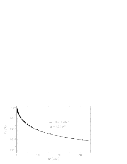
Figure 2: Theoretical results (solid line) versus corrected experimental Brash data on $F_{1}(Q^{2})$

From the two leading power corrections in the OPE, without gluon exchange, the one proportional to the quark condensate does not contribute to $F_{1}(Q^{2})$, while the other, proportional to the four-quark condensate, has a vanishing double discontinuity in the $(s,s^{\prime})$ complex plane. For details see the original article Dom05 .

In order to extract $F_{2}(Q^{2})$, we have to consider the leading-order non-perturbative corrections to the OPE, which in this case corresponds to the quark condensate.

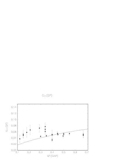
Figure 3: Experimental data on $G_{E}(Q^{2})$ for the neutron jeff , together with the theoretical results

In the case of the proton, the contribution involving the up-quark condensate vanishes (due to vanishing traces) and therefore we only have a piece proportional to $\langle\bar{d}d\rangle$. Our choice of Lorentz structure in this case is $/\!\!\!q\gamma^{\mu}$, which appears in the QCD sector as well as in the hadronic sector multiplying $F_{2}(Q^{2})$ but not $F_{1}(Q^{2})$. We refer to the original article Dom05 for the full expressions. Here we will give only the final result that emerges form the FESR

$$F_{2}(Q^{2})=-\frac{\langle\bar{d}d\rangle}{24\kappa_{p}\,M_{N}\,\pi^{2}\,\lambda_{N}^{2}}[2s_{0}(Q^{2}+s_{0})$$

$$+\,Q^{2}\,(Q^{2}+2s_{0})\,\ln(\frac{Q^{2}}{Q^{2}+2s_{0}})]\;.$$ (16)

The problem is that the asymptotic behavior does not agree with the expectations. We find

$$\lim_{Q^{2}\rightarrow\infty}F_{2}(Q^{2})=-\frac{\langle\bar{d}d\rangle}{18\kappa_{p}\,M_{N}\,\pi^{2}\,\lambda_{N}^{2}}$$

$$\times(\frac{s_{0}^{3}}{Q^{2}}-\frac{s_{0}^{4}}{Q^{4}}+...)\;,$$ (17)

and we would expect $F_{2}(Q^{2})$ to fall faster than $F_{1}(Q^{2})$ at least by a factor of $1/Q$ JLABF2 . A comparison of $F_{2}(Q^{2})$ from equation $(16)$ with data shows a disagreement at the level of a factor two, which cannot be improved adjusting the values of $\lambda$ and $s_{0}$. The main reason behind the disagreement is the soft $q^{2}$-dependence of $F_{2}(Q^{2})$.

We can do the same analysis for the neutron form factors. It turns out that $F_{1n}(Q^{2})$ for the neutron is numerically very small and consistent with zero, except near $Q^{2}=0$ due to the divergence in the chiral limit. Since $F_{1n}(Q^{2})\approx 0$, the Sachs form factor is proportional to $F_{2n}(Q^{2})$. In Fig.3 we show a plot of the electric Sachs form factor for the neutron. At low $Q^{2}$ there is reasonable agreement with the experimental data. However, for higher momentum transfers the disagreement turns out to be serious due to the soft $1/Q^{2}$ behavior of $F_{2n}(Q^{2})$.

Acknowledgements: We acknowledge support fom Fondecyt under grants 1051067 and 7050125

References

• (1) For a review see e.g. V.L. Chernyak, I.R. Zhitnitsky, Phys. Rep. 112 (1984) 173.
• (2) V.M. Braun, A. Lenz, N. Mahnke and E. Stein, Phys. Rev. D 65 (2002) 074011; A. Lenz, M. Wittmann and E. Stein, Phys. Lett. B 581 (2004) 199
• (3) For a recent review see e.g. P. Colangelo, A. Khodjamirian, in ”At the frontiers of particle physics, Handbook of QCD, Vol. 3, 1495, M.A. Shifman, ed., (World Scientific, Singapore, 2001).
• (4) For a review see e.g. L.J. Reinders, H. Rubinstein, S. Yazaki, Phys. Rep. 127 (1985) 1.
• (5) C.A. Dominguez, M. Loewe, Z. Phys. C 58 (1993) 273.
• (6) B.L. Ioffe, Nucl. Phys. B 188 (1981) 817; E: B 191 (1981) 591.
• (7) C.A. Dominguez, M. Loewe, J.S. Rozowsky, Phys. Lett. B 335 (1994) 506.
• (8) J. Arrington, Phys. Rev. D 68 (2003) 034325; Phys. Rev. C 69 (2004) 022201.
• (9) E. J. Brash, A. Kozlov, S. Li and G. M. Huber, Phys. Rev. D 65 (2002) 022201.
• (10) H. Castillo, C. A. Dominguez and M. Loewe, JHEP 03 (2005)012.
• (11) JEFFERSON LAB E93-026 collaboration, G. Warren et al., Phys. Rev. Lett. 92 (2004) 04301 and references therein.