Dynamically Warped Theory Space and Collective Supersymmetry Breaking

Abstract:

We study deconstructed gauge theories in which a warp factor emerges dynamically and naturally. We present nonsupersymmetric models in which the potential for the link fields has translational invariance, broken only by boundary effects that trigger an exponential profile of vacuum expectation values. The spectrum of physical states deviates exponentially from that of the continuum for large masses; we discuss the effects of such exponential towers on gauge coupling unification. We also present a supersymmetric example in which a warp factor is driven by Fayet-Iliopoulos terms. The model is peculiar in that it possesses a global supersymmetry that remains unbroken despite nonvanishing D-terms. Inclusion of gravity and/or additional messenger fields leads to the collective breaking of supersymmetry and to unusual phenomenology.

1 Introduction

The possibility exists that there are spatial dimensions beyond the three that we are able to perceive. However, gauge theories in extra dimensions are not renormalizable and are to be understood as effective theories. An example of an ultraviolet completion of extra-dimensional gauge theories is provided by deconstruction [1, 2]. In this approach, one arranges the action of a four-dimensional gauge theory so that at low energies it reproduces the action of a five-dimensional theory that is latticized in one spatial dimension. The high-energy theory can be asymptotically free, with fermions condensing at an intermediate scale to provide the link fields of the latticized theory [1]. At energies below the scale at which the condensation occurs (which still must be significantly higher than the inverse size of the extra dimension) the theory is effectively described by a “moose” theory in which scalar link fields obtain vacuum expectation values (vevs) [2]. The spectrum of fields in the spontaneously-broken theory is designed to mimic the Kaluza-Klein (KK) towers of the higher-dimensional theory.

Deconstructed extra dimensions have proven useful for building the features of higher-dimensional phenomenology into four-dimensional models. Examples include the little Higgs models of electroweak symmetry breaking [3], extra-dimensional grand unified theories [4] and models of supersymmetry (SUSY) breaking [5, 6, 7, 8, 9, 10].

Deconstruction has also provided a new handle on nonperturbative effects in higher-dimensional supersymmetric theories and string compactifications [11, 12]. The novel latticizations which arise in studies of deconstruction have led to new approaches in latticizing chiral gauge theories [13] and supersymmetric theories [14]. The deconstruction of theories with higher-dimensional gravity has not been completely successful, but has provided insight into the scales at which gravitational modes in a latticized theory become strongly coupled [15]. In addition, deconstruction of warped extra dimensions [16, 17] has allowed for an explicit realization of the holographic renormalization group [18] and the transition between logarithmic and power-law running of couplings as a function of energy [19].

Most deconstructed extra-dimensional models are fine tuned in the sense that the gauge couplings at each lattice site and the vevs of the link fields must be fixed precisely in order to reproduce the dynamics of an extra dimension. We will study some theories in which a warped theory space is generated dynamically, without a significant fine-tuning of parameters. To this end, we impose an approximate hopping symmetry in the link field potential, which would render our theories invariant under translations if our moose were infinitely long. We allow the form of the hopping potential to vary at the ends of our finite moose, as a way of taking into account effects that could reasonably occur at the boundaries in the continuum theory. With these assumptions, we will see that an exponential profile of link field vevs can occur naturally for a wide range of model parameters, precisely what one needs to deconstruct models with bulk fields in Anti-de Sitter (AdS) space.

In contrast to the spectra obtained in the continuum theory, however, we find towers of gauge and link field states whose masses grow exponentially with KK number. This suggests a concrete way to distinguish the four-dimensional models that we study from those that genuinely live in a warped extra dimension. If the standard model exists in the bulk of the deconstructed extra dimension, we will see that unification occurs at least as well as in the nonsupersymmetric standard model, but at an accelerated rate due to the Kaluza-Klein modes.

We then turn to supersymmetric moose models that dynamically generate warp factors. We focus on a U(1)ⁿ theory in which a Fayet-Iliopoulos term for each gauge factor forces vevs for neighboring link fields to vary monotonically along the lattice, except at the boundary. What is intriguing about this model is that each U(1) factor has a nonvanishing D term, yet the low-energy theory remains globally supersymmetric, as we will see by studying the spectra of the gauge and link fields. We explain how this unusual circumstance is possible, and then add mediating fields and gravity, leading to nonsupersymmetric spectra. The collective SUSY breaking in the extended theory shares some features with Scherk-Schwarz SUSY breaking [20] and twisted theory space [7], but is also different from those types of models in several important ways. In the absence of the mediating fields, global SUSY remains unbroken, as opposed to the usual situation in which mediating fields have a tendency to restore SUSY. Also, SUSY breaking here is of the “supersoft” type [21] because there are no fields which obtain F-term vevs. However, the suppression of the SUSY breaking scale with respect to the vacuum energy yields a gravitino that is heavy in these models.

Our paper is organized as follows. In Section 2 we review the framework of deconstructed extra dimensions and theory space. In Section 3 we study dynamically generated nonsupersymmetric warped extra dimensions. We study gauge coupling running in these deconstructed theories and compare with the continuum theory and with the Standard Model. In Section 4 we study the dynamically deconstructed supersymmetric U(1) theory and its unusual SUSY breaking phenomenology. We conclude in Section 5.

2 Framework

In this section we review the deconstruction of a warped extra dimension. It is important to note that the gauge theories we eventually study are more correctly described as models in “theory space”, i.e., the space of four-dimensional theories that can be described conveniently by moose diagrams. For particular values of the link field vevs and gauge couplings, the theory space will coincide at low energies with a latticized extra dimension. It will be of particular interest to us when this correspondence reproduces the spectrum and interactions of a gauge theory in AdS space, at least in the continuum limit.

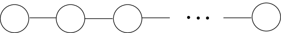
Figure 1: A linear moose.

Consider an $n$-site moose diagram with $n$ SU(N) gauge groups connected by $n-1$ link fields $\phi_{i}$, as shown in Fig. 1. The link fields transform in the bifundamental representation under neighboring groups. The action of our moose diagram is

$$S=\int d^{4}x\sum_{i}\left[-\frac{1}{2}\hbox{Tr}\left[F^{\mu\nu}_{i}F^{i}_{\mu\nu}\right]+\hbox{Tr}|D_{\mu}\phi_{i}|^{2}\right]\,$$ (1)

where $F^{\mu\nu}_{i}$ is the non-Abelian field strength for the $i^{th}$ group, and $\phi_{i}$ is the link field connecting the $i^{th}$ and $(i+1)^{th}$ site. (We leave it implicit that the sum runs up to $n$ in the first term and $n-1$ in the second term.) The covariant derivative of $\phi_{i}$ is given by,

$$D_{\mu}\phi_{i}=\partial_{\mu}\phi_{i}+iq\,A_{\mu}^{i}\phi_{i}-iq\,\phi_{i}A_{\mu}^{i+1}.$$ (2)

Note that $F_{\mu\nu}\equiv F_{\mu\nu}^{a}T^{a}$, where $T^{a}$ is a group generator, satisfying $\mbox{Tr}(T^{a}T^{b})=\delta^{ab}/2$. (In the Abelian case we will take the generators to be the identity, so that $\mbox{Tr}(T^{2})=1$). To compare the moose theory with the lattice gauge theory action it is useful to express Eq. (1) using a nonlinear field redefinition of the bifundamental fields $\phi_{j}$:

$$\phi_{j}=v_{j}\,U(j,j+1) \equiv v_{j}\,\exp\left[iqa\,A_{5}^{j}\right]$$ (3)

$$\approx v_{j}\,(1+iqaA_{5}^{j}+\cdots)\,,$$

where we have expressed the $j^{th}$ link in terms of a “comparator” field $U$. The parameter $a$ has units of length, and the exponential in the field redefinition represents the Wilson line along the interval $(y_{j},y_{j}+a)$ in the extra dimension. With this choice, the action for the link fields may be written to quadratic order in $A_{5}$ as,

$$S = \int d^{4}x\sum_{i}q^{2}v_{i}^{2}a^{2}\mbox{Tr}|\partial_{\mu}A_{5}^{i}-\frac{(A^{i+1}_{\mu}-A_{\mu}^{i})}{a}+iq\,(A_{\mu}^{i}A_{5}^{i}-A_{5}^{i}A_{\mu}^{i+1})|^{2}$$ (4)

$$= \int d^{4}x\sum_{i}q^{2}v_{i}^{2}a^{2}\mbox{Tr}|\partial_{\mu}A_{5}^{i}-\frac{(A^{i+1}_{\mu}-A_{\mu}^{i})}{a}+iq\,[A_{\mu}^{i},A_{5}^{i}]-iqA_{5}^{i}(A_{\mu}^{i+1}-A_{\mu}^{i})|^{2}$$

We can compare this to the action of a warped five-dimensional theory,

$$S=\int\,d^{4}x\,dy\sqrt{g}\,\left(-\frac{1}{2}\mbox{Tr}[F^{\mu\nu}F_{\mu\nu}]-\mbox{Tr}[F^{\mu 5}F_{\mu 5}]\right)\,,$$ (5)

where the metric is of the form

$$ds^{2}=e^{-f(y)}dx^{2}+dy^{2}\,.$$ (6)

We now discretize this action on a lattice with $n$ sites and spacing $a$, so that the length of the extra dimension in these coordinates is $R=na$. This requires that we make the substitutions

$$F^{\mu\nu}(x^{\rho},y)\rightarrow F^{\mu\nu}_{i}(x^{\rho})\,,\,\,\,\,\,\,f(y)\rightarrow f_{i}\,,$$ (7)

$$\int dy\rightarrow\sum_{i}a\,\,\,,$$ (8)

$$\partial_{5}A^{\mu}\rightarrow\frac{A_{i+1}^{\mu}-A_{i}^{\mu}}{a}\,\,\,,$$ (9)

so that our five-dimensional action becomes

$$S=\sum_{i}a\int d^{4}x\,\left[-\frac{1}{2}\mbox{Tr}(F_{i}^{\mu\nu})^{2}+e^{-f_{i}}\,\mbox{Tr}\left(\partial_{\mu}A_{i}^{5}-\frac{A^{i+1}_{\mu}-A^{i}_{\mu}}{a}+iq\,[A_{\mu}^{i},A_{5}^{i}]\right)^{2}\right]\,\,\,.$$ (10)

Thus we recover the action of the moose model, up to terms of higher order in the lattice spacing $a$, provided we identify

$$v_{i}=\frac{e^{-f_{i}/2}}{qa}\,\,\,.$$ (11)

The exercise above demonstrates how the geometry of an extra dimension may be encoded in the profile of link field vevs in the four-dimensional theory. For AdS space, one has $f_{j}=2kaj$, where $k$ is the AdS curvature, and one finds that $v_{j+1}=\exp(-ka)\,v_{j}$. In the next section, we present nonsupersymmetric models in which such a profile of vevs is generated dynamically. In these models, the potential for the link fields will have the form

$$V=V_{b}\,(\phi_{1})+\sum_{i=1}^{n-1}V_{i}\,(\phi_{i},\phi_{i+1})\,,$$ (12)

with $\phi_{n}\equiv 0$, corresponding to a Dirichlet boundary condition. The second term in Eq. (12) is invariant under translations $i\rightarrow i+1$ along the moose, except at the boundaries $i=1$ and $i=n-1$. We may choose $V_{b}(\phi_{1})$ so that the explicit breaking of this translation invariance triggers a monotonically varying profile of link vevs. We show in the next section that generic forms exist for the hopping terms $V_{i}$ that provide for local minima with the desired properties, without requiring an unnatural choice of parameters.

The deconstruction of warped supersymmetric theories is similar to the example just considered, except that each site corresponds to an ${\cal N}=1$ vector multiplet, and each link to a chiral multiplet. Aside from the vector multiplet that includes the zero mode gauge field, the remaining $n-1$ massive multiplets include both a vector and chiral superfield, each transforming as an adjoint under the unbroken diagonal subgroup. This is consistent with our expectation that the KK levels arising from an underlying 5D theory should form ${\cal N}=2$ SUSY multiplets. Each bi-fundamental link field also contains a singlet under the unbroken gauge group, but these states are generally assumed to have no impact on the low-energy phenomenology. In our explicit treatment of the link potential, the spectra of all physical states will be specified in our models.

3 Non-supersymmetric Warped Theory Space

In this section, we consider non-supersymmetric examples of the class of theories described in Section 2. These theories dynamically generate a warp factor that becomes exponential in the limit that the number of sites $n$ is taken large. We determine the spectrum of link and gauge fields that appear in such models later in this section.

3.1 Non-supersymmetric Models

Let us begin by considering nonsupersymmetric U(1)ⁿ gauge theories, with gauge couplings $g_{i}=g$ and $n-1$ link fields with charges

$$\phi_{i}\sim(+1,-1)\,\,\,,$$ (13)

under the $i^{th}$ and $(i+1)^{th}$ group factors, respectively. We wish to find potentials of the form (12) that will generate a warp factor. As a warm up, consider the following fine-tuned example,

$$V_{b}=(a_{1}-m^{2})^{2}\,\,\,,$$ (14)

and

$$V_{i}=(\lambda\,a_{i}-a_{i+1})^{2}\,\,\,.$$ (15)

where $a_{i}=\phi_{i}^{\dagger}\phi_{i}$, for $i=1\dots n-1$, and $a_{n}=0$. This model is fine-tuned in the sense that the terms appearing in the potential are not the most general set allowed by the symmetries of the theory. We discuss more general examples afterwards. The advantage of the model defined by Eqs. (14) and (15) is that it allows us to extract a number of useful results without resorting to numerical analysis.

Since we are looking for solutions in which all the $\phi$ develop vevs, we may minimize $V$ with respect to the $a_{i}$. Excluding the links at the ends of the moose, the minimization condition for the $\ell^{th}$ link is simply

$$(1+\lambda^{2})\,a_{\ell}-\lambda\,(a_{\ell+1}+a_{\ell-1})=0\,\,\,.$$ (16)

Given the translation invariance of the system, it is not hard to show that a general solution is given by

$$a_{j}=A\,\exp(Kj)+B\,\exp(-Kj)$$ (17)

where

$$\cosh K=\frac{1+\lambda^{2}}{2\lambda}\,\,\,.$$ (18)

The minimization conditions on $a_{1}$ and $a_{n-1}$ both differ from Eq. (16),

$$(1+\lambda^{2})\,a_{1}-m^{2}-\lambda\,a_{2}=0\,\,\,,$$ (19)

$$-\lambda\,a_{n-2}+(1+\lambda^{2})\,a_{n-1}=0\,\,\,.$$ (20)

and determine the coefficients $A$ and $B$. After some algebra, the general solution in Eq. (17) can be reduced to

$$a_{j}=\frac{m^{2}}{\lambda}\left(\frac{1}{1-\lambda^{2n}}\,\lambda^{j}+\frac{1}{1-\lambda^{-2n}}\,\lambda^{-j}\right)\,\,\,,$$ (21)

for $j=1\ldots n-1$.

This solution provides the desired warp factor, providing it corresponds to, at least, a local minimum of the potential. For our choice $\lambda<1$, one sees that in the $n\rightarrow\infty$ limit Eq. (21) reduces to

$$a_{j}=m^{2}\,\lambda^{j-1},$$ (22)

since the second term approaches $-\lambda^{2n-j}$, which is vanishing for all $j$. For finite $n$, one finds monotonically decreasing link vevs. For example, in the case where $n=4$ (i.e., three link fields) and $\lambda=0.3$ one finds

$$v_{1}=1.00\,m,\,\,\,\,\,\,\,\,\,\,v_{2}=0.55\,m,\,\,\,\,\,\,\,\,\,\,v_{3}=0.29\,m,$$ (23)

where $v_{i}=\langle a_{i}\rangle^{1/2}$. Note that the U(1)ⁿ gauge invariance allows us to choose all of the $v_{i}$ real and positive.

Without working out the mass spectrum of the link fields explicitly, we may nonetheless show that the extremum of the potential just described is at least a local minimum. First we note that in the $n\rightarrow\infty$ limit, the solution Eq. (22) corresponds to $V(\{\langle\phi_{i}\rangle\})=0$. However, the potential is clearly positive definite and there are no flat directions. We therefore conclude that our solution in the $n\rightarrow\infty$ limit corresponds to a global minimum.

For $n$ finite, consider the scalar mass squared matrix

$$m^{2}_{ij}=\left(\frac{\partial^{2}V}{\partial\xi_{i}\xi_{j}}\right)_{min}=\left(\frac{\partial^{2}V}{\partial a_{k}\partial a_{\ell}}\frac{\partial a_{k}}{\partial\xi_{i}}\frac{\partial a_{\ell}}{\partial\xi_{j}}\right)_{min}\,\,\,,$$ (24)

where $\xi_{i}$ represents the real and imaginary components of the link fields in the basis

$$\xi=(\phi_{1}^{im},\phi_{2}^{im},\ldots,\phi_{n-1}^{im},\phi_{1}^{re},\phi_{2}^{re},\ldots,\phi_{n-1}^{re})\,\,\,.$$ (25)

For $1\leq i\leq n-1$ or $1\leq j\leq n-1$, the factors $\partial a/\partial\xi$ are vanishing, since the vevs of the $\phi_{i}$ are purely real. This implies that there are $n-1$ zero eigenvalues, corresponding to the goldstone boson degrees of freedom in the spontaneous breaking of U(1)${}^{n}\rightarrow$U(1). Only the lower-right $(n-1)\times(n-1)$ block of the Eq. (24) is nonvanishing, and is of the form

$$m^{2}=VA\,V^{T}\,\,\,,$$ (26)

where $V$ is a diagonal matrix of vacuum expectation values $V=diag(v_{1},v_{2},\ldots v_{n-1})$, and $A$ is a dimensionless matrix of the form

$$A=\left(\begin{array}[]{cccccc}(1+\lambda^{2})&-\lambda&&&&\\ -\lambda&\,(1+\lambda^{2})&-\lambda&&&\\ &&&&\ddots&\\ &&&&-\lambda&(1+\lambda^{2})\end{array}\right)\,\,\,.$$ (27)

Since $V$ is nonsingular, it follows that the number of positive eigenvalues of $m^{2}$ and $A$ are the same. Therefore, it is sufficient that we show that $A$ has only positive eigenvalues. The proof is as follows: For $\lambda=0$, $A$ is the identity matrix, which is clearly positive definite. As we allow $\lambda$ to vary continuously away from zero, the only way any eigenvalue can become negative is for there to exist a value of $\lambda$ for which that eigenvalue vanishes and the determinant of $A$ is zero. However, one can verify that

$$\det A=1+\sum_{j=1}^{n-1}\lambda^{2j}\,\,\,,$$ (28)

which is never vanishing. Thus, all the eigenvalues of $A$, and hence $m^{2}$, remain positive for arbitrary $\lambda$. Our warped solution corresponds to a minimum of the potential.

As we have commented earlier, the potential we have just examined is not the most general one that we could have written down. Ignoring the currently fashionable trend of settling for fine-tuned models, we now turn to more general possibilities. Assuming renormalizable, next-to-nearest-neighbor interactions, the most general form for the $V_{i}$ in a U(1)ⁿ theory is

$$V_{i}(\phi_{i},\phi_{i+1})=\hat{m}^{2}a_{i}+\lambda\,a_{i}^{2}+\rho a_{i}\,a_{i+1}\,\,\,.$$ (29)

As before, we assume the boundaries of the moose are special, and include the additional corrections

$$V_{b}(\phi_{1})=-m_{1}^{2}a_{1}+\lambda_{1}a_{1}^{2}\,\,\,,$$ (30)

designed to trigger a vacuum expectation value at one end of the moose. In this general parameterization, the four-site example that gave us Eq. (23) corresponds to $m_{1}^{2}=2m^{2}$, $\lambda_{1}=0$, $\hat{m}^{2}=0$, $\lambda=1.09$, and $\rho=-0.6$. By varying these parameters continuously away from our successful, yet fine-tuned, solution we can find more general results. For example, the parameter choice $\lambda_{1}=-0.8$, $\hat{m}^{2}=0.4$, $\lambda=1.0$, and $\rho=-0.7$ we obtain a local minimum with

$$v_{1}=1.78\,m_{1},\,\,\,\,\,\,\,\,\,\,v_{2}=0.98\,m_{1},\,\,\,\,\,\,\,\,\,\,v_{3}=0.37\,m_{1}\,\,\,.$$ (31)

For large $n$, where end effects become less important in determining the location of the minimum, one can find parameter choices that yield viable warped solutions for arbitrary $n$. To illustrate this point, we have studied numerically the potential defined by Eqs. (29) and (30) for $n$ ranging from $30$ to $100$. The results, which we have verified correspond to minima of the potential, are shown in Fig. 2.

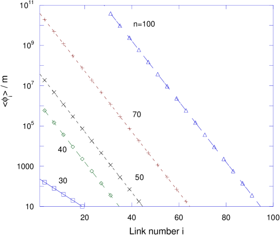
Figure 2: Link field vevs for $n=30$, $40$, $50$, $70$ and $100$. The solutions shown correspond to the parameter choices $m_{1}^{2}=2m^{2}$, $\lambda_{1}=-0.8$, $\lambda=1$, and $\rho=-0.8$.

It is clear by inspection that the vevs have the desired approximate exponential dependence on link number. Also note that there is no significant fine-tuning in the choice of parameters $m_{1}^{2}=2m^{2}$, $\lambda_{1}=-0.8$, $\lambda=1$, and $\rho=-0.8$. While other successful solutions are possible, we will not survey the parameter space.

We instead turn to models that may have somewhat different phenomenological applications, namely those involving non-Abelian group factors. We are interested in SU(N)ⁿ moose that are broken to the diagonal SU(N) while spontaneously generating a warp factor. Defining the SU(N)${}_{i}\times$SU(N)_i+1 invariant combinations,

$$a_{i}=\mbox{Tr}({\phi_{i}}^{\dagger}\phi_{i})\,,\,\,\,\,b_{i}=\mbox{Tr}({\phi_{i}}^{\dagger}\phi_{i}{\phi_{i}}^{\dagger}\phi_{i})\,,\,\,\,\,c_{i}=\mbox{Tr}({\phi_{i}}^{\dagger}\phi_{i}\phi_{i+1}{\phi_{i+1}}^{\dagger})\,\,\,,$$ (32)

we study the potential

$$V_{i}=\tilde{m}^{2}a_{i}+\tilde{\lambda}\,a_{i}^{2}+\tilde{\lambda}^{\prime}b_{i}+\tilde{\rho}\,a_{i}\,a_{i+1}+\tilde{\eta}\,c_{i}\,\,\,,$$ (33)

$$V_{b}=-\tilde{m}_{1}^{2}\,a_{1}+\tilde{\lambda}_{1}\,a_{1}^{2}\,\,\,,$$ (34)

where, again, boundary corrections have been added to trigger spontaneous symmetry breaking. To facilitate our numerical analysis of the potential, we choose $N=3$, since SU(3) is the smallest SU(N) group that retains many of same group theoretical properties of larger SU(N) (for example, non-vanishing $f^{abc}$ and $d^{abc}$ constants). It is possible to duplicate the warp factors shown in Fig. 2 in the non-Abelian case, provided that we make the parameter identifications

$$\tilde{m}_{1}^{2}=m_{1}^{2}/3\,\,\,\,\,\tilde{\lambda}_{1}=\lambda_{1}/9\,\,\,\,\,\tilde{m}^{2}=m^{2}/3\,\,\,\,\,9\tilde{\lambda}+3\tilde{\lambda}^{\prime}=\lambda\,\,\,\,\,9\tilde{\rho}+3\tilde{\eta}=\rho\,\,\,.$$ (35)

For $\tilde{\lambda}=\tilde{\lambda}^{\prime}=\lambda/12$ and $\tilde{\rho}=\tilde{\eta}=\rho/12$ we have found numerically that our warped extrema remain stable minima of the enlarged potential Eqs. (33) and (34). The results of Fig. 2 can thus be applied to study the gauge boson spectrum in both Abelian and non-Abelian examples.

Gauge boson masses originate from the link kinetic terms

$${\cal L}_{m}=\sum_{j}^{n-1}\,\mbox{Tr}\left(D_{\mu}\phi_{j}\right)^{\dagger}\left(D^{\mu}\phi_{j}\right)\,\,\,,$$ (36)

which reduce to

$$g^{2}\sum_{j}^{n-1}v_{j}^{2}\,\mbox{Tr}\left[A_{j+1}\cdot A_{j+1}-2\,A_{j+1}\cdot A_{j}+A_{j}\cdot A_{j}\right]\,\,\,,$$ (37)

where $g$ is the gauge coupling, or in matrix form

$$m^{2}_{gauge}=g^{2}\left(\begin{array}[]{ccccccc}\quad v^{2}_{1}&\quad-v^{2}_{1}&&&&&\\ -v^{2}_{1}&v^{2}_{1}+v^{2}_{2}&-v^{2}_{2}&&&&\\ &-v^{2}_{2}&v^{2}_{2}+v^{2}_{3}&-v^{2}_{3}&&&\\ &&&&\ddots&\\ &&&&&v^{2}_{n-2}+v^{2}_{n-1}&-v^{2}_{n-1}\\ &&&&&-v^{2}_{n-1}&v^{2}_{n-1}\end{array}\right)\,\,.$$ (38)

For the warped solutions shown in Fig. 2, it is straightforward to evaluate the eigenvalues of Eq. (38) numerically. Results for the Abelian, $n=100$ model are shown in Fig. 3.

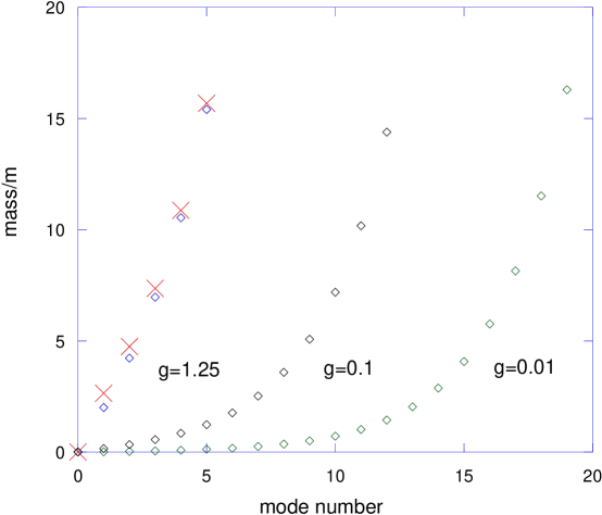
Figure 3: Mass spectra of the scalar and vector states for the Abelian $n=100$ model, for $g=0.01$, $0.1$ and $1.25$. Gauge (link) field states are indicated by diamonds (crosses).

A number of comments are in order. While the gauge tower has a zero mode (corresponding to the unbroken U(1) factor), the scalar tower has an “almost” zero mode whose mass approaches zero in the limit $n\rightarrow\infty$. This mode can be identified as the pseudo-goldstone boson of the broken approximate translation invariance of the moose. In the Abelian models, this state (as well as every other in its tower) is a gauge singlet and does not necessarily portend any inescapable phenomenological problems. However, more precise statements can only be made in the context of specific phenomenological applications. For the other scalar and vector modes, which we will label by an integer $k\geq 1$, the mass spectra in Fig. 3 are very accurately described by the exponential functions,

$$m_{k}^{s} = 2.711\,m\,e^{0.347\,k}$$

$$m_{k}^{v} = 2.086g\,m\,e^{0.348\,k}\,\,\,,$$ (39)

where $s$ and $v$ indicate the scalar and vector masses, respectively. For the particular value $g\approx 1.25$, the two towers of states become nearly degenerate. In Reference [22], it was shown that the product of nonzero eigenvalues of the mass matrix Eq. (38) is given by,

$$\prod_{i}m_{i}^{2}=N\prod_{i}g^{2}v_{i}^{2}.$$ (40)

If the vevs $v_{i}$ vary exponentially, then (40) leads one to conjecture that the masses may have an exponential spectrum for most of the tower, as we have found numerically. Assuming a tower of the form $m_{j}\sim[\exp(-kR)/a]\exp(kaj)$, where $k$ is the AdS scale and $a$ is the lattice spacing, we expect the exponential to approximate the roughly linear tower of the continuum theory for the first ${\cal O}(ka)$ modes. It is useful to compare these results explicitly to the spectrum of bulk scalar and vector modes in a 5D slice of anti-de Sitter space. Defining the parameter $x_{n}$ by

$$m_{n}=x_{n}\,k\,\exp(-kr_{c}\pi)\,\,\,,$$ (41)

where $k$ is the AdS curvature and $r_{c}$ is the compactification radius, the values of $x_{n}$ for a massless bulk scalar are given by [23]

$$2\,J_{\nu}(x_{n})+x_{n}\,J^{\prime}_{\nu}(x_{n})=0\,\,\,,$$ (42)

with $\nu=2$, and for a bulk U(1) gauge field by [24]

$$J_{1}(x_{n})+x_{n}\,J^{\prime}_{1}(x_{n})+\alpha_{n}[Y_{1}(x_{n})+x_{n}\,Y^{\prime}_{1}(x_{n})]=0\,\,\,,$$ (43)

where $J$ and $Y$ are Bessel functions, and

$$\alpha_{n}\approx-\frac{\pi}{2}[\ln(x_{n}/2)-kr_{c}\pi+\gamma+1/2]^{-1}\,\,\,.$$ (44)

Note that $\gamma\approx 0.577$ is the Euler constant, and the Eqs. (42), (43) and (44) are accurate provided that $\exp(-kr_{c}\pi)\ll 1$. The values of $x_{n}$ can be obtained numerically, and increase approximately linearly with $n$. For simplicity, we can compare this spectrum to our original, fine-tuned model where $a_{i}\approx m^{2}\lambda^{j-1}$, with $\lambda$ set to $1/2$. Assuming the phenomenologically motivated value $kr_{c}\approx 11.27$ (to generate the Planck scale/weak scale hierarchy) and the choice $m\approx 5\times 10^{-12}k$ (to match the light KK spectrum of the continuum theory), we obtain the first few modes shown in Fig. 4.

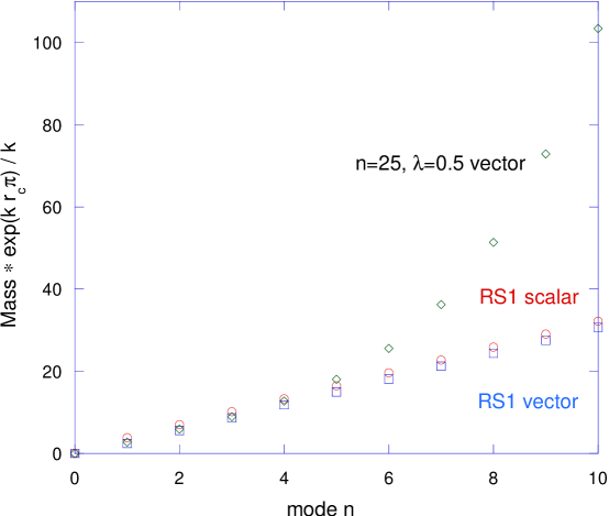
Figure 4: Comparison of the spectra of our simplified deconstructed model to the continuum results Eqs. (42) and (43), assuming $\lambda=1/2$, $m\approx 5\times 10^{-12}k$ and $kr_{c}\approx 11.27$. See the text for discussion.

It is therefore possible that the deconstructed models presented here can effectively mimic the first few gauge Kaluza-Klein modes of the Randall-Sundrum model, even with a coarse-grained lattice (i.e. large lattice spacing). As one would expect, fine lattices do a better job of reproducing continuum results. As an example, let us assume the hierarchy $v_{n-1}/v_{1}=e^{-k\pi r_{c}}=e^{-30}$. Since $\pi r_{c}=na$ we identify the AdS scale, $k=(k\pi r_{c})/(na)=30/(na)$. We also identify the lattice spacing, $a^{-1}=gv_{1}$, where we have chosen to shift the warp factor so that $f(y_{1})=0$. This choice corresponds to $\lambda=e^{-60/(n-1)}=0.985$ for $n=4000$ in the parametrization of the mass matrix used earlier. To summarize, the mapping of continuum parameters to lattice parameters in this model is $k=30gv_{1}/n$ and $\pi r_{c}=n/(gv_{1})$. In Fig. 5 we consider a relatively fine lattice with 4000 lattice sites and compute the spectrum of gauge boson masses; there is relatively good agreement between this result and that of the continuum. Whether or not there is a continuum interpretation of the models we consider over a large range of energies, our warped deconstructed models are interesting in their own right, as we will describe in the following sections.

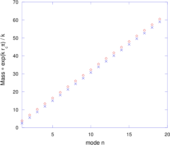
Figure 5: Comparison of the continuum (crosses) and the deconstructed gauge boson spectrum for $4000$ lattice sites (diamonds), in units of $k\exp(-k\pi r_{c})$ with $k\pi r_{c}=30$.

Finally, we comment on the scalar mass spectrum of the non-Abelian models. We have already noted that the potential given in Eqs. (33) and (34) generate warp factors, and we identified solutions that are minima of the potential. We note here that the bifundamentals decompose under the diagonal gauge group into a real adjoint which is eaten; and a real adjoint and complex singlet which remain in the physical spectrum. The uneaten fields do not necessarily have an extra dimensional interpretation. (The adjoints are necessary in the supersymmetric version of the theory to form KK modes of a 5D SUSY multiplet.) The $n-1$ singlets under the diagonal gauge group remain massless and are identified with the Goldstone bosons of the spontaneously broken U(1)^n-1 global symmetry acting on the $\phi_{i}$. One may include SU(N)_i-invariant operators like

$$\Delta V_{i}=c\,M^{4-N}\,\det\phi_{i}+\mbox{h.c.}$$ (45)

with small coefficient $c$, and the $n-1$ singlet states in question will become massive without spoiling the pattern of link field vevs obtained in the absence of these terms. It is also worth noting that higher-dimension operators that break the translation invariance of the moose can be included to raise the mass of the lightest adjoint scalar state.

3.2 Gauge Coupling Running

There are many possible applications of the nonsupersymmetric warped deconstructed theories that we have just considered. For example, one could construct purely four-dimensional analogs of the warped theories that attempt to explain fermion masses via bulk wave function overlaps [25]. Whatever the application, one is bound to ask how the mass spectra described in the previous section affect gauge coupling running and unification [26]. We consider that issue in this section.

We begin with the generic observation that the towers of gauge and link fields that we obtained were well approximated by

$$m_{0}=0\,\,\,\,\,\mbox{and}\,\,\,\,\,m_{j}=\bar{m}e^{\bar{a}\,j},\,j\geq 1\,$$ (46)

when the number of sites was large. Here, the parameter set $(\bar{m},\bar{a})$ corresponds to a particular towers of states, and may differ between the gauge and uneaten link fields. We will simplify our discussion by assuming that these parameters are universal. However, as we noted earlier, the link degrees of freedom that are not eaten by the gauge fields could have a different spectrum. While the gauge tower has an exact zero mode, we assume that the lightest link field modes (which are real scalar fields in the adjoint representations of the diagonal, non-Abelian gauge groups) are heavy enough to evade direct detection, but can be taken as massless as far as the renormalization group running is concerned. This is equivalent to saying that we ignore any low-scale threshold effects.

For simplicity, let us consider the effect of a single field with an exponential tower of modes on the running of a diagonal gauge coupling. Imagine that we start at some initial renormalization scale $\mu_{0}$ and evolve the gauge coupling $\alpha$ through each KK mass threshold up to a scale $\mu$ that is given by $m_{N}\leq\mu\leq m_{N+1}$. One finds that

$$\alpha^{-1}(\mu)=\alpha^{-1}(\mu_{0})-\frac{b}{2\pi}\ln\frac{m_{1}}{\mu_{0}}-\sum_{j=2}^{N}\frac{j\,b}{2\pi}\ln\frac{m_{j}}{m_{j-1}}-\frac{(N+1)\,b}{2\pi}\ln\frac{\mu}{m_{N}}\,,$$ (47)

where $b$ is the one-loop beta function. The exponential form of the spectrum for the massive modes in the KK towers leads to a simplification of the logarithms in Eq. (47), which in turn allows us to do the sum in the third term. The result is

$$\alpha^{-1}(\mu)=\alpha^{-1}(\mu_{0})-\frac{b}{2\pi}\ln\frac{\mu}{\mu_{0}}-\frac{N\,b}{2\pi}\ln\frac{\mu}{\bar{m}}+\frac{\bar{a}\,b}{4\pi}N(N+1)\,\,\,.$$ (48)

The first two terms give the usual one-loop renormalization group running of the couplings between the scales $\mu_{0}$ and $\mu$; the last two terms are corrections due to the particular form of our KK towers. To understand the effect of these terms, it is useful to note that for large $N$, $N(N+1)\approx N^{2}\approx(\ln\frac{\mu}{\bar{m}}/\bar{a})^{2}$. Thus, unlike gauge coupling running in the standard model, Eq. (48) has a quadratic dependence on the log of the renormalization scale.

This point has been noted before in studies of gauge coupling running in deconstructed AdS space [26]. The presence of log squared terms arises due to the choice of boundary conditions on the gauge couplings. In our models, we define the gauge couplings to have a common value at a common scale, which can be identified as the scale of the highest link field vev. This choice is required by the assumed translation invariance of our theories. However, to reproduce the purely logarithmic gauge coupling evolution expected in AdS space, one must define each gauge coupling of the deconstructed theory at the scale of the corresponding link vev, before setting the couplings equal [26]. In the framework that we have presented, there is no symmetry of the four-dimensional theory that would make such a choice natural. We therefore use Eq. (48) to draw our phenomenological conclusions.

Let us now apply Eq. (48) to the standard model. We take $\mu_{0}=m_{Z}$ and the gauge couplings $\alpha^{-1}_{1}=59.02$, $\alpha^{-1}_{2}=29.57$ and $\alpha^{-1}_{3}=8.33$. Our SU(3), SU(2) and U(1) beta function contributions are

$$\begin{array}[]{lcl}\mbox{gauge (massless)}&\mbox{ }&(-11,-22/3,0)\\ \mbox{gauge (massive)}&&(-21/2,-7,0)\\ \mbox{physical links}&&(1/2,1/3,0)\\ \mbox{matter}&&(4,4,4)\\ \mbox{Higgs}&&(0,1/6,1/10)\end{array}$$ (49)

One sees that the sum of massless gauge, higgs and matter beta functions in Eq. (49) is $(-7,-19/6,41/10)$, the usual result in the standard model with one electroweak Higgs doublet. As a further check, one can also note that the sum of Higgs plus massive gauge beta functions is $(-21/2,-41/6,1/10)$, which agrees with the KK beta function given in Ref. [19] for the nonsupersymmetric standard model with only the gauge fields and one Higgs doublet in the bulk. In the present application, the beta functions multiplying the $\ln(\mu/\mu_{0})$ term in Eq. (48) are the sum of the Higgs, matter, physical link, and massless gauge beta functions shown in Eq. (49), $(-13/2,-17/6,41/10)$; the beta function contributions of each KK level is the sum of the physical link and massive gauge beta functions, $(-10,-20/3,0)$. As an example, the choice $\bar{a}=1$ and $\bar{m}=1$ TeV leads to unification at the scale $7\times 10^{5}$ GeV with

$$\frac{\alpha^{-1}_{3}-\alpha^{-1}_{12}}{\alpha^{-1}_{12}}=11.8\%,$$ (50)

where $\alpha^{-1}_{12}$ is evaluated at the point where the SU(2) and U(1) couplings unify. This is not terribly impressive, but should be put in the appropriate context. Unification in the nonsupersymmetric standard model occurs at $1\times 10^{13}$ GeV with

$$\frac{\alpha^{-1}_{3}-\alpha^{-1}_{12}}{\alpha^{-1}_{12}}=13.4\%$$ (51)

using the input numbers defined earlier. Thus, the existence of the exponential towers of gauge and link states actually improves unification slightly in comparison to the minimal standard model. This is significant since we had no reason a priori to expect that approximate unification would be possible at all. From a practical point of view, this suggests that any of a number of possible corrections to standard model unification (for example, those motivated by split supersymmetry) could correct this result as needed. We do not pursue this possibility further here.

4 Deconstructed Warped SUSY and Collective SUSY Breaking

In this section we consider models with global supersymmetry. We dynamically deconstruct a warped 5D supersymmetric U(1) gauge theory, and discuss the unusual properties and phenomenology of this model. Related models were studied in [8, 9, 10].

4.1 The Deconstructed SUSY U(1) Theory

The 4D theory is an ${\cal N}$=1 supersymmetric moose theory. Unlike our previous examples, the U(1) gauge fields now belong to vector multiplets with the associated gauginos, and the link fields $\phi_{i}$ are chiral multiplets with charges $(+1,-1)$ under neighboring gauge groups. To avoid gauge anomalies we can use the Green-Schwarz mechanism or add Wess-Zumino terms. The structure of the anomaly-canceling sector of the theory is tightly constrained if the theory is to appear extra dimensional in the limit of small lattice spacing [8]. We will not concern ourselves with the details of this sector of the theory, but rather cancel anomalies by introducing a duplicate set of link fields $\overline{\phi}$, but with opposite charges $(-1,+1)$, resulting in the quivers of Figure 6. The additional bifundamentals have no extra dimensional interpretation, but they also are singlets under the low-energy U(1) gauge symmetry and for most practical purposes can be ignored. In the following, we will include the doubled set of link fields with the understanding that one of the two sets will not have a higher-dimensional interpretation.

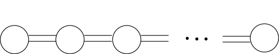
Figure 6: Moose for the supersymmetric U(1)ⁿ theory. Doubled links indicate chiral superfields with charges $(+1,-1)$ and $(-1,+1)$.

Warping of the extra dimensions in the Abelian theory can be accomplished through the addition of Fayet-Iliopoulos (FI) terms $\xi_{i}$. The potential for the scalar link fields arises from the D-terms, and is given by:

$$V_{D}=\sum_{i=1}^{n}D_{i}^{2},$$ (52)

where,

$$D_{i}=g\left(|\phi_{i}|^{2}-|\phi_{i-1}|^{2}-|\overline{\phi}_{i}|^{2}+|\overline{\phi}_{i-1}|^{2}+\xi_{i}\right).$$ (53)

As usual, for a circular moose we define $\phi_{0}=\phi_{n}$ and for the interval (orbifold) moose we define $\phi_{0}=\phi_{n}=0$ (and similarly for $\overline{\phi}_{0}$ and $\overline{\phi}_{n}$). We will again focus on the orbifold theory. We assume for now that the superpotential vanishes, so that the only contribution to the scalar potential is due to the D-terms.

The stationary points of the D-term potential satisfy,

$$\left<\phi_{i}\right>\,\left(\left<D_{i}\right>-\left<D_{i+1}\right>\right)=0\ .$$ (54)

The vacua generically have equal D-terms, with,

$$\left<D_{i}\right>=\frac{\sum_{j}g\xi_{j}}{n}\equiv D.$$ (55)

As a result, the scalar VEVs $v_{i}$ and $\overline{v}_{i}$ satisfy the recursion relation,

$$(|v_{i+2}|^{2}-|\overline{v}_{i+2}|^{2})-2(|v_{i+1}|^{2}-|\overline{v}_{i+1}|^{2})+(|v_{i}|^{2}-|\overline{v}_{i}|^{2})=(\xi_{i+1}-\xi_{i+2})\ .$$ (56)

The U(1)ⁿ gauge symmetry is generically broken to a diagonal U(1). The second set of link fields does not alter this symmetry breaking pattern because the link fields are neutral under the unbroken U(1). There are flat directions in the potential for which $|\phi_{i}|^{2}$ and $|\overline{\phi}_{i}|^{2}$ are shifted by the same constant $c_{i}$. These flat directions correspond to the $n-1$ moduli $\overline{\phi}_{i}\phi_{i}$. For simplicity in what follows, we will assume $\overline{v}_{i}=0$, and we will use the gauge symmetry to make the $v_{i}$ real. None of the following results changes qualitatively if we allow for $\overline{\phi}_{i}$ vevs. Alternatively, as discussed earlier, we can remove the $\overline{\phi}$ chiral multiplets from the theory and include Wess-Zumino terms in the action to cancel the gauge anomalies.

One amusing consequence of supersymmetry in this theory is that the spectrum of massive chiral multiplets is the same as the spectrum of massive vector multiplets, as required in order to mimic the KK spectrum of a supersymmetric 5D gauge theory. The SUSY Higgs mechanism forces the scalar masses to equal the gauge boson masses, resulting in a 4D ${\cal N}$=2 supersymmetric spectrum of massive fields [5].

Notice that the relation between scalar VEVs (56) is a latticized form of the equation,

$$\frac{\partial^{2}|\phi(y)|^{2}}{\partial y^{2}}=-\frac{\xi^{\prime}(y)}{a},$$ (57)

where $a$ is a lattice spacing that will be defined in terms of the fundamental parameters of the theory shortly. The explicit ultraviolet dependence in the continuum scalar field equation could be absorbed in a redefinition of the FI terms, but we will not do that here. Equation (57) can be integrated once to give,

$$\frac{\partial|\phi(y)|^{2}}{\partial y}=\frac{-\xi(y)+D/g}{a},$$ (58)

with integration constant $D/g$, which is the continuum form of (55) with $D_{i}$ given by (53) and

$$D/g=\int_{0}^{R}dy\,\xi(y)/R.$$ (59)

Equation (58) relates the warp factor of (6) to the 4D Fayet-Iliopoulos terms:

$$\frac{\partial e^{-f(y)}}{\partial y}=(-g^{2}\xi(y)+gD)a.$$ (60)

The warp factors that can be obtained in this way form a restricted class. As a particular example, if all of the FI terms are equal then from (58) with $\xi(y)=D/g=const$, the warp factor is constant and the metric reproduces flat spacetime. As another example, if the first of the FI terms differs from the rest, then the right-hand side of (58) is constant in $y$ except at the special site with unique FI term (corresponding to a delta function in the continuum limit). The resulting (squared) warp factor $e^{-f(y)}$ has a linear profile.

More generally, we note that according to (55) each D-term is equal to the average value of $g\xi_{j}$, which in the continuum limit becomes

$$D=g\int_{0}^{R}dy\,\frac{\xi(y)}{R}.$$ (61)

Then, suppose we want to fix the right-hand side of (58) so as to reproduce a particular warp factor, so that

$$\xi(y)=\widetilde{\xi}(y)+D/g=\widetilde{\xi}(y)+\int_{0}^{R}dy\,\xi(y)/R,$$ (62)

for some specified profile $\widetilde{\xi}(y)$. Whether or not there is a solution to the integral equation (62) depends on the choice of $\widetilde{\xi}(y)$. To determine the constraint on $\widetilde{\xi}(y)$ we integrate (62) over $y$ and find,

$$\int_{0}^{R}dy\,\widetilde{\xi}(y)=0.$$ (63)

Hence, we learn that in order to obtain a monotonic warp factor, there must be a delta function contribution to $\xi(y)$ at a boundary of the spacetime. We can also see the difficulty in obtaining a monotonic warp factor by recognizing that $\widetilde{\xi}(y)$ is the difference between $\xi(y)$ and its average value over the interval $(0,R)$. As a result, if $\widetilde{\xi}(y)>0$ for some y, then there must exist some $y^{\prime}$ where $\xi(y^{\prime})<0$. The same argument applies to the latticized theory: If for some $i$, $(\xi_{i}-D/g)>0$ then there exists an $i^{\prime}$ for which $(\xi_{i^{\prime}}-D/g)<0$. Then, by Eqs. (53) and (55), in order for the warp factor to be monotonic, the FI term $\xi_{1}$ at the boundary will differ in sign from the FI terms in the bulk. (In fact, we will see in Section 4.3 that $\widetilde{\xi}(y)$ is the profile of FI terms in an equivalent theory with vanishing vacuum energy.)

4.2 The KK spectrum

The masses of the components of the vector and chiral multiplets arise from the Kähler potential for the bifundamental chiral multiplets,

$${\cal L}\supset\int d^{4}\theta\,\sum_{i}\Phi_{i}^{\dagger}\,\exp\left[g(V_{i}-V_{i+1})\right]\,\Phi_{i}+\overline{\Phi}_{i}^{\dagger}\,\exp\left[g(-V_{i}+V_{i+1})\right]\,\overline{\Phi}_{i},$$ (64)

where $\Phi_{i}$ is the bifundamental chiral multiplet charged under U(1)_i+1 and U(1)_i, and $V_{i}$ is the U(1)_i vector multiplet. We will separately calculate the gauge boson, scalar, and fermion masses, and find that the spectrum is supersymmetric despite the nonvanishing D-terms in the vacuum. Later we will explain why the presence of global supersymmetry is to be expected, and we will study the unusual SUSY breaking phenomenology of this and related models.

4.2.1 Gauge bosons

On the supersymmetric orbifold, as in the nonsupersymmetric case, the gauge boson masses arise from the bifundamental vevs through the Higgs mechanism, with mass terms,

$${\cal L}\supset\frac{1}{2}A_{i\,\mu}M_{ij}A_{j}^{\mu}\ .$$ (65)

The mass-squared matrix is, as before,

$$m_{\rm gauge}^{2}=2g^{2}\left(\begin{array}[]{ccccccc}v_{1}^{2}&&-v_{1}^{2}&&&&\\ -v_{1}^{2}&&v_{1}^{2}+v_{2}^{2}&&-v_{2}^{2}&&\\ &&-v_{2}^{2}&&v_{2}^{2}+v_{3}^{2}&-v_{3}^{2}&\\ &&&&\ddots&\ddots&\\ &&&&&-v_{n-1}^{2}&\ v_{n-1}^{2}\end{array}\right)$$ (66)

Identifying the lattice spacing with $a\equiv 1/(gv_{1})$ as in the nonsupersymmetric theory, we recover the spectrum of gauge fields in a latticized warped extra dimension with metric,

$$ds^{2}=e^{-f(y)}dx^{2}+dy^{2}\ ,$$ (67)

with warp factor $e^{-f(na)}=v_{n}/v_{1}$. The action of the continuum theory then includes,

$$S\supset\int d^{5}x\left(-\frac{1}{4}F_{MN}F^{MN}\right).$$ (68)

The relative factor of two between Equations (66) and (38) is due to our normalization of the generators in the Abelian and non-Abelian theories. We have chosen $\rm{Tr}\,T^{a}T^{b}=c\delta_{ab}$ with $c=1/2$ for the non-Abelian theory, but $c=1$ for the Abelian theory.

4.2.2 Fermions

The Kähler potential for the chiral multiplets couples the chiral multiplets to the gauginos, and gives rise to the following mass terms in the fermion Lagrangian:

$${\cal L} \supset i\frac{g}{\sqrt{2}}\,\sum_{i}\left[\lambda_{i}(v_{i}\psi_{i}-v_{i-1}\psi_{i-1})-\overline{\lambda}_{i}(\overline{\psi}_{i}-\overline{\psi}_{i-1})\right]\$$ (69)

$$= i\frac{g}{\sqrt{2}}\,(\lambda_{i}\ |\ \psi_{i})\ \left(\begin{array}[]{c|c}&\ \Theta\\ \hline\cr\Theta^{\dagger}&\end{array}\right)_{ij}\ \left(\begin{array}[]{c}\lambda_{j}\\ \hline\cr\psi_{j}\end{array}\right)\ +\ {\rm h.c.},$$ (74)

where the $n\times(n-1)$ dimensional matrix $\Theta$ is,

$$\Theta=\left(\begin{array}[]{cccc}v_{1}&&&\\ -v_{1}&v_{2}&&\\ &\ddots&\ddots&\\ &&-v_{n-2}&v_{n-1}\\ &&&-v_{n-1}\end{array}\right)\ .$$ (75)

The fermion mass matrix is identified by writing the fermion Lagrangian in the form,

$${\cal L}\supset\frac{1}{2}\,(\lambda_{i}\ |\ \psi_{i})\ M_{ij}\left(\begin{array}[]{c}\lambda_{j}\\ \hline\cr\psi_{j}\end{array}\right)\ +\ {\rm h.c.}$$ (76)

The squared mass matrix is the given by,

$$M^{2}_{\rm fermions}=2g^{2}\left(\begin{array}[]{cc}\Theta\Theta^{\dagger}&\\ &\Theta^{\dagger}\Theta\end{array}\right)\ .$$ (77)

The block diagonal elements of the mass matrix are proportional to,

$$\Theta\Theta^{\dagger} = \left(\begin{array}[]{ccccc}v_{1}^{2}&-v_{1}^{2}&&&\\ -v_{1}^{2}&\ v_{1}^{2}+v_{2}^{2}&-v_{2}^{2}&&\\ &-v_{2}^{2}&v_{2}^{2}+v_{3}^{2}&-v_{3}^{2}&\\ &&\ddots&\ddots&\\ &&&-v_{n-1}^{2}&v_{n-1}^{2}\end{array}\right)\,,$$ (83)

$$\Theta^{\dagger}\Theta = \left(\begin{array}[]{ccccc}2v_{1}^{2}&-v_{1}v_{2}&&&\\ -v_{1}v_{2}&2v_{2}^{2}&-v_{2}v_{3}&&\\ &-v_{2}v_{3}&2v_{3}^{2}&-v_{3}v_{4}&\\ &&\ddots&\ddots&\\ &&&-v_{n-2}v_{n-1}&2v_{n-1}^{2}\end{array}\right)\ .$$ (89)

The upper-left diagonal block of the mass squared matrix $M^{2}_{\rm fermions}$ is identical to the gauge boson mass matrix. The bottom right diagonal block has identical eignenvalues to the first, except that the zero mode is missing from that sector. The single fermion zero mode is therefore composed entirely of the gauginos:

$$\lambda\equiv\frac{1}{\sqrt{n}}\sum_{i=1}^{n}\lambda_{i}.$$ (90)

This zero mode will be important later in the discussion of SUSY breaking. The massive modes match the spectrum of massive gauge bosons, as required for 5D supersymmetry.

4.2.3 Scalars

The scalar masses are determined by the D-term potential Eq. (53). Defining $d_{i}\equiv\left<D_{i}\right>=v_{i}^{2}-v_{i-1}+\xi_{i}$, and $\phi_{i}=v_{i}+\varphi_{i}$, we may expand,

$$V_{D} = g^{2}\sum_{i}\left[(\varphi_{i+1}+v_{i+1})(\varphi_{i+1}^{\dagger}+v_{i+1})-(\varphi_{i}+v_{i})(\varphi_{i}^{\dagger}+v_{i})-|\overline{\phi}_{i+1}|^{2}+|\overline{\phi}_{i}|^{2}+\xi_{i+1}\right]^{2}$$

$$= g^{2}\sum_{i}\left[d_{i+1}+|\varphi_{i+1}|^{2}+v_{i+1}\,(\varphi_{i+1}^{\dagger}+\varphi_{i+1})-|\varphi_{i}|^{2}-v_{i}\,(\varphi_{i}^{\dagger}+\varphi_{i})-|\overline{\phi}_{i+1}|^{2}+|\overline{\phi}_{i}|^{2}\right]^{2}\,,$$

from which if follows that

$$V_{D}\supset 2g^{2}\sum_{i}(d_{i}-d_{i+1}) \left(|\varphi_{i}|^{2}+v_{i}\,(\varphi_{i}^{\dagger}+\varphi_{i})-|\overline{\phi}_{i}|^{2}\right)$$

$$+g^{2}\sum_{i}\left(v_{i+1}(\varphi_{i+1}^{\dagger}+\varphi_{i+1})-v_{i}(\varphi_{i}^{\dagger}+\varphi_{i})\right)^{2}$$

$$=2g^{2}\sum_{i}(d_{i}-d_{i+1}) \left(|\varphi_{i}|^{2}+v_{i}\,(\varphi_{i}^{\dagger}+\varphi_{i})-|\overline{\phi}_{i}|^{2}\right)$$ (93)

$$+\frac{1}{2}(\varphi_{i}^{\dagger}\ |\ \varphi_{i})\,g^{2}\left(\begin{array}[]{c|c}\Theta^{\dagger}\Theta&\ \Theta^{\dagger}\Theta\\ \hline\cr\Theta^{\dagger}\Theta&\ \Theta^{\dagger}\Theta\end{array}\right)\left(\begin{array}[]{c}\varphi_{i}\\ \hline\cr\varphi_{i}^{\dagger}\end{array}\right)\ ,$$

where $\Theta^{\dagger}\Theta$ is the same matrix that determines the fermion masses Eq. (89). We will see again in Section 4.3 that the D-terms in the vacuum, $d_{i}$, are all equal, so that the terms in (93) proportional to $(d_{i}-d_{i+1})$ vanish.

Diagonalizing the mass matrix, the imaginary modes $(\varphi_{i}-\varphi_{i}^{\dagger})$ have vanishing masses, and are the $n-1$ eaten Goldstone modes of the U(1)${}^{n}\rightarrow$U(1) gauge symmetry breaking pattern. The real modes have the same masses as the massive fermions and gauge bosons. The $\overline{\phi}_{i}$ fields remain massless, and do not have a higher-dimensional interpretation.

The 5D vector multiplet is decomposed into a tower of massive 4D vector multiplets, consisting of a massive gauge boson, two Weyl fermions and a real scalar; it includes, in addition, a massless vector multiplet and chiral multiplet, consisting of a massless gauge boson, two Weyl fermions, and a complex scalar. In the continuum theory, by allowing the orbifold action on the fields to include a transformation by an element of the R-symmetry of the supersymmetric theory, supersymmetry can be partly or completely broken. The “boundary conditions,” specified by the terms in the Lagrangian from the first and last site of the moose, project out one massless Weyl fermion and one massless complex scalar, leaving an ${\cal N}$=1 vector multiplet zero mode consisting of a massless gauge boson and Weyl fermion. (We could have kept an extra zero-mode chiral multiplet by adding an additional chiral multiplet charged under the first U(1) gauge group in the moose and not giving its scalar component a vev.) Hence, we have found a spectrum of gauge bosons, fermions and scalars consistent with 5D supersymmetry partially broken to 4D SUSY at the zero-mode level by the orbifold boundary conditions. The U(1) D-terms do not vanish in the vacuum, so the fact that we have recovered a supersymmetric low-energy theory may at first sight seem surprising. This is the subject of the next section.

4.3 SUSY Without Supergravity

Unless the FI terms are fine-tuned such that $\sum_{i}\xi_{i}=0$, then by Eq. (55) the D-terms cannot simultaneously vanish and it would seem that there should then be a collective breaking of supersymmetry from the nonvanishing D-term VEVs. In fact this is not the case, as we have seen that the spectrum of the deconstructed U(1) orbifold theory preserves four supercharges (${\cal N}$=1 in 4D). The reason this is possible is that only the unbroken diagonal U(1) has a nonvanishing FI term,

$$\xi_{\rm diag}=\frac{1}{\sqrt{n}}\sum_{i}\xi_{i}\ .$$ (94)

All linear combinations of U(1)’s orthogonal to the diagonal U(1) have vanishing FI terms by orthogonality and the equality of the D-term VEVs $d_{i}$.

The diagonal U(1) has no charged matter, so the FI term is just a cosmological constant and can be shifted away (until we couple the theory to gravity). To see this explicitly, we define,

$$\widetilde{\xi}_{i}\equiv\xi_{i}-\frac{\sum_{i}\xi_{i}}{n}\ ,$$ (95)

and

$$\widetilde{D}_{i}\equiv g\left(|\phi_{i}|^{2}-|\phi_{i-1}|^{2}-|\overline{\phi}_{i}|^{2}+|\overline{\phi}_{i-1}|^{2}+\widetilde{\xi}_{i}\right)\ ,$$ (96)

after which the D-term potential becomes

$$V_{D}=\sum_{i}\widetilde{D}_{i}^{2}+\frac{\left(\sum_{i}\xi_{i}\right)^{2}}{n}\ .$$ (97)

We have defined $\widetilde{\xi}_{i}$ such that $\sum_{i}\widetilde{\xi}_{i}=0$. Hence, the deconstructed U(1) theory with arbitrary FI terms is equivalent to a theory with FI terms $\widetilde{\xi}_{i}$ in which global SUSY is unbroken (according to Eq. (55)) plus a cosmological constant $\Lambda=(\sum_{i}\xi_{i})^{2}/n$.

According to the usual definition of the supersymmetry transformations, the Goldstino transforms non-homogeneously. This is usually taken to be the indicator of supersymmetry breaking. However, in this theory we can redefine the action of the SUSY generators on the gauginos such that the non-homogeneous part of the SUSY transformed Goldstino is shifted away. The Goldstino is identified with the massless fermion mode of (90), $\lambda=\sum_{i}\lambda_{i}/\sqrt{n}$. The Goldstino is composed entirely of gauginos, as expected in the absence of F-terms. Its SUSY transformation is,

$$\delta\lambda=i\epsilon\frac{\sum_{i}D_{i}}{\sqrt{n}}+\sigma^{\mu\nu}\epsilon\frac{\sum_{i}{F_{\mu\nu}^{i}}}{\sqrt{n}}\ ,$$ (98)

where $\epsilon$ is the superspace parameter and $\sigma^{\mu\nu}=1/4\,[\sigma^{\mu},\sigma^{\nu}]$ with $\sigma^{\mu}$ the Pauli matrices for $\mu=1,2,3$ and $\sigma^{0}=-1$. The vacuum value of the D-term part of the transformation rule makes the gaugino transform non-homogeneously, which is usually taken to be the indicator of SUSY breaking. However, if we shift the D-terms by their VEVs, we find that the following SUSY transformation is also preserved by this theory:

$$\widetilde{\delta}\lambda=i\frac{\sum_{i}\widetilde{D}_{i}}{\sqrt{n}}+\sigma^{\mu\nu}\epsilon\frac{\sum_{i}{F_{\mu\nu}^{i}}}{\sqrt{n}}\ .$$ (99)

The vacuum part of the $\widetilde{\rm D}$-term part vanishes by definition, so that the would-be Goldstino transforms homogeneously under the shifted SUSY transformation. The SUSY transformation rule for the shifted auxiliary fields $\widetilde{D}_{i}$ is the same as for the original auxiliary fields $D_{i}$,

$$\widetilde{\delta}\widetilde{D}_{i}=\delta D_{i}=\overline{\epsilon}\,\overline{\sigma}^{\mu}\partial_{\mu}\lambda_{i}-\epsilon\sigma^{\mu}\partial_{\mu}\overline{\lambda}_{i}.$$ (100)

We are free to shift the supersymmetry transformations in this way because the diagonal D-term is independent of the matter fields in this theory, and its SUSY transformation depends only on derivatives of the gauginos so that the additional shift of the gauginos by a constant does not affect the transformation of the D-term. Once again, we are only able to shift the SUSY transformations in this theory because there is no charged matter under the diagonal U(1) gauge symmetry which has nonvanishing D-term. Otherwise the shifted SUSY would not be a symmetry of the theory because of the dependence of the auxiliary D-term on the charged fields. Also, when we couple the theory to gravity we will no longer be able to redefine the supersymmetry in a similar way because the positive vacuum energy breaks local supersymmetry.

4.4 SUSY-breaking Phenomenology

Despite the unbroken global SUSY identified above, SUSY breaking reappears when the supersymmetric U(1) theory is coupled to gravity or a messenger sector. In this case, one finds the unusual feature that the scales of SUSY breaking in the messenger and in the gravity sector may be hierarchically different. This result is obtained because the supersymmetry is broken collectively: if any one of the D-terms conditions were removed, then there would be a supersymmetric ground state. The supersymmetry breaking is therefore nonlocal in nature and, from the 5D perspective, corresponds to including an explicit position-dependent cosmological constant in the theory by hand. However, one should not take this interpretation too literally, as we have not deconstructed 5D gravity. It should be clear, though, that this situation is unlike models of deconstructed Scherk-Schwarz SUSY breaking or radion F-term SUSY breaking [27]. In those cases the boundary conditions break global supersymmetry, while here we preserve supersymmetry without supergravity.

If we are willing to give up on the higher-dimensional interpretation of the model, then we may assign random Fayet-Iliopoulos terms to the $n$ U(1) factors in the theory. The central limit theorem leads to an expected value of $\sum_{i}\xi_{i}$ which grows like $\sqrt{n}$ for large number of lattice sites. Now we can imagine coupling one of the U(1) factors in the moose to the MSSM through messenger fields. If we define the typical scale for the $\xi_{i}$ to be $\hat{\xi}$ and take $g\sqrt{\hat{\xi}}\sim M_{Pl}$ then the SUSY breaking scale as seen by the messengers and the splitting of messenger masses would be of size,

$$M_{\rm SUSY}^{2}=\left<D_{i}\right>=\frac{g^{2}\sum_{i}\xi_{i}}{n}\sim\frac{g^{2}\hat{\xi}}{n^{1/2}}\sim\frac{M_{Pl}^{2}}{n^{1/2}}\ .$$ (101)

Gravity, on the other hand, would communicate a SUSY breaking scale specified by the cosmological constant,

$$M_{\rm grav}^{2}=\left(\sum_{i}D_{i}^{2}\right)^{1/2}\sim g^{2}\xi\sim M^{2}_{Pl}\ ,$$ (102)

and gravitino mass,

$$m_{3/2}=M_{\rm grav}^{2}/M_{Pl}\sim M_{Pl}\ .$$ (103)

The suppression of the collectively broken SUSY scale by the number of lattice sites in (101) is reminiscent of the suppressed scalar mass in little Higgs theories [3], although in the present case the suppression is a tree level effect. It is also reminiscent of a related model, studied in Ref. [8], in which SUSY is broken by a deconstructed Wilson line and Fayet-Iliopoulos terms at the boundary. The collective SUSY breaking in that model gives rise to a suppressed SUSY breaking scale at the first lattice site because the D-terms themselves are warped in that model. This is as opposed to the present theory, in which the D-terms are equal along the lattice.

We can mediate the SUSY breaking via heavy messengers $T$ and $\overline{T}$ connecting the first lattice site to the MSSM, as in Figure 7. If we give the messengers a large mass compared to the scale of the light modes (but potentially $\ll M_{Pl}$), then the D-term at the first lattice site splits the squared masses of the scalar fields in $T$ and $\overline{T}$ by an amount $\pm 2\left<D_{1}\right>$. Fermion masses remain unchanged at tree level.

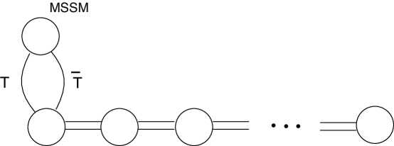
Figure 7: Schematic representation of the coupling of the U(1)ⁿ theory to the MSSM (or gauge extended MSSM) via the messenger fields $T$ and $\bar{T}$.

Because SUSY breaking is governed by D-terms, the collective D-term breaking in our model only generates supersoft SUSY breaking terms [21]. As exposited in [21], in the MSSM coupled to a D-term SUSY breaking sector, SUSY breaking scalar masses first arise by a dimension-ten operator. If the gauge sector of the MSSM is enhanced to that of ${\cal N}$=2 SUSY in 4D, then additional SUSY breaking operators are possible, including supersoft Dirac gaugino masses $\sim D/M$ and supersoft scalar squared masses $\sim D^{2}/M^{2}$. These operators are called supersoft because they do not give rise to log divergences in scalar masses or in other operators. The phenomenology of such models is interesting and, with the extended gauge sector, the spectrum of the theory interpolates between that of gaugino mediation and gauge mediation [21]. However, due to the collective SUSY breaking in our U(1) moose model, the phenomenology here is somewhat different. To examine this, we extend the MSSM gauge sector by adding MSSM adjoint chiral multiplets $A$, enhancing the gauge sector to the content of ${\cal N}$=2 SUSY multiplets.

F-terms can couple the messengers to the adjoint chiral multiplets of the extended gauge sector of the MSSM via a Lagrangian of the form,

$$\int d^{2}\theta\,\left(MT\overline{T}+\alpha TA\overline{T}\right)\ .$$ (104)

Here we assume that $A$ has vanishing VEVs so that the MSSM gauge symmetry is not broken by the adjoint scalars. Then $T$ and $\overline{T}$ do not obtain VEVs, so the U(1) $D$ term VEVs are unchanged by the presence of the messenger fields. Integrating out the messengers through diagrams containing the D-term vev gives rise to supersoft scalar and gaugino masses [21]. However, because of the hierarchy in this model between the vacuum energy and the D-term at each site, the gravitino need not be the lightest SUSY particle even if $M\ll M_{Pl}$ with weak scale supersoft gaugino masses $\sim\left<D_{1}\right>/M\sim m_{W}$, since $m_{3/2}\sim\sum_{i}\left<D_{i}\right>/M_{Pl}\gg\left<D_{1}\right>/M_{Pl}$ for a large moose. This is unlike the generic supersoft theory in which a single D-term governs the scale of SUSY breaking masses in both the MSSM and the supergravity sector and the gravitino can be naturally light.

5 Conclusions

Deconstruction provides a new paradigm for creating four-dimensional gauge theories. At some points in the space of link field vevs, a deconstructed theory may have a simple description as the latticized version of a gauge theory in a higher-dimensional space. At other points, there may be no simple correspondence, but the theory may nonetheless possess some interesting phenomenological features of its extra-dimensional cousins. Much of the literature has focused on deconstructed flat extra dimensions, in which all the link fields have equal vevs, while somewhat less attention has been directed toward warped spaces. In either case, the origin of the link field vevs and the mechanism that provides naturally for a warping of the theory space have met little scrutiny. We have studied a number of explicit models to shed light on these issues.

In our nonsupersymmetric constructions, we have seen that a combination of translation invariance in the bulk and boundary corrections to the link field potential are often sufficient to generate an exponential profile for the link field vevs. In these examples, the bulk potential depends only on a few parameters and could be taken general in form, aside from the constraint of translation invariance. Local minima of the potential could be found that exhibited the desired warping, without a significant fine-tuning of parameters. The physical spectra of gauge and link fields consists of exponential towers, with a ‘pseudo-zero mode’ for the link tower corresponding to the broken approximate translational invariance of the moose. The mass of this state can be raised by including appropriate higher-dimension operators. We found that the first few states in these towers can mimic the results expected for anti-de Sitter space, but that the spectra overall deviate exponentially from the expected linear dependence on mode number. Perhaps the most exciting possibility in these models is that this deviation could be discerned at a future collider. In this case, one could learn whether the physics observed corresponds to an underlying theory space or to a new physical space.

In the supersymmetric case, we focused primarily on an Abelian theory, where the warping was accomplished via Fayet-Iliopoulos D-terms that forced the squares of the link field vevs to grow by an additive factor as one moves along the moose. Aside from providing an existence proof of supersymmetric versions of the type of models of interest to us, this U(1)ⁿ model is particularly interesting in the way that supersymmetry breaking occurs non-locally: without all $n$ $D$-flatness constraints (involving all of the $n-1$ link fields) there would be supersymmetric vacua. In its simplest form, the model has the peculiar feature that supersymmetry breaking appears only via the generation of a cosmological constant, while the spectra of the physical gauge and link states remains supersymmetric. In the case where the moose is allowed to couple to additional matter, the delocalization of supersymmetry breaking implies that fields localized at a single site experience a source of supersymmetry-breaking, $D_{i}^{2}$, that is $1/n$ as strong as the full amount available for gravity mediation leading, for example, to a heavy gravitino. In addition, supersymmetry breaking is supersoft in this scenario. These features may make our U(1)ⁿ model distinctive if it is applied as a secluded supersymmetry-breaking sector for the minimal supersymmetric standard model.

The models we have presented suggest a path for building more realistic and economical models in warped theory space. The construction of useful warped non-Abelian supersymmetric moose models and a study of the full standard model embedding in this framework are directions worthy of future study.

References

- [1] N. Arkani-Hamed, A. G. Cohen and H. Georgi, “(De)constructing dimensions,” Phys. Rev. Lett. 86, 4757 (2001) [arXiv:hep-th/0104005].
- [2] C. T. Hill, S. Pokorski and J. Wang, “Gauge invariant effective Lagrangian for Kaluza-Klein modes,” Phys. Rev. D 64, 105005 (2001) [arXiv:hep-th/0104035].
- [3] N. Arkani-Hamed, A. G. Cohen and H. Georgi, “Electroweak symmetry breaking from dimensional deconstruction,” Phys. Lett. B 513, 232 (2001) [arXiv:hep-ph/0105239]; N. Arkani-Hamed, A. G. Cohen, T. Gregoire and J. G. Wacker, “Phenomenology of electroweak symmetry breaking from theory space,” JHEP 0208, 020 (2002) [arXiv:hep-ph/0202089]; N. Arkani-Hamed, A. G. Cohen, E. Katz, A. E. Nelson, T. Gregoire and J. G. Wacker, “The minimal moose for a little Higgs,” JHEP 0208, 021 (2002) [arXiv:hep-ph/0206020]; N. Arkani-Hamed, A. G. Cohen, E. Katz and A. E. Nelson, “The littlest Higgs,” JHEP 0207, 034 (2002) [arXiv:hep-ph/0206021].
- [4] N. Weiner, “Unification without unification,” arXiv:hep-ph/0106097; H. C. Cheng, K. T. Matchev and J. Wang, “GUT breaking on the lattice,” Phys. Lett. B 521, 308 (2001) [arXiv:hep-ph/0107268]; N. Arkani-Hamed, A. G. Cohen and H. Georgi, “Accelerated unification,” arXiv:hep-th/0108089; P. H. Chankowski, A. Falkowski and S. Pokorski, “Unification in models with replicated gauge groups,” JHEP 0208, 003 (2002) [arXiv:hep-ph/0109272]; C. Csaki, G. D. Kribs and J. Terning, “4D models of Scherk-Schwarz GUT breaking via deconstruction,” Phys. Rev. D 65, 015004 (2002) [arXiv:hep-ph/0107266]. C. D. Carone, “Tri-N-ification,” Phys. Rev. D 71, 075013 (2005) [arXiv:hep-ph/0503069].
- [5] C. Csaki, J. Erlich, C. Grojean and G. D. Kribs, “4D constructions of supersymmetric extra dimensions and gaugino mediation,” Phys. Rev. D 65, 015003 (2002) [arXiv:hep-ph/0106044].
- [6] H. C. Cheng, D. E. Kaplan, M. Schmaltz and W. Skiba, “Deconstructing gaugino mediation,” Phys. Lett. B 515, 395 (2001) [arXiv:hep-ph/0106098].
- [7] N. Arkani-Hamed, A. G. Cohen and H. Georgi, “Twisted supersymmetry and the topology of theory space,” JHEP 0207, 020 (2002) [arXiv:hep-th/0109082].
- [8] A. Falkowski, H. P. Nilles, M. Olechowski and S. Pokorski, “Deconstructing 5D supersymmetric U(1) gauge theories on orbifolds,” Phys. Lett. B 566, 248 (2003) [arXiv:hep-th/0212206]; E. Dudas, A. Falkowski and S. Pokorski, “Deconstructed U(1) and supersymmetry breaking,” Phys. Lett. B 568, 281 (2003) [arXiv:hep-th/0303155].
- [9] K. R. Dienes, E. Dudas and T. Gherghetta, “A calculable toy model of the landscape,” Phys. Rev. D 72, 026005 (2005) [arXiv:hep-th/0412185].
- [10] T. Kobayashi, N. Maru and K. Yoshioka, “4D construction of bulk supersymmetry breaking,” Eur. Phys. J. C 29, 277 (2003) [arXiv:hep-ph/0110117]; H. Abe, T. Kobayashi, N. Maru and K. Yoshioka, “Field localization in warped gauge theories,” Phys. Rev. D 67, 045019 (2003) [arXiv:hep-ph/0205344]; N. Maru and K. Yoshioka, “Sparticle masses in product-group gauge theories,” Eur. Phys. J. C 31, 245 (2003) [arXiv:hep-ph/0311337].
- [11] C. Csaki, J. Erlich, V. V. Khoze, E. Poppitz, Y. Shadmi and Y. Shirman, “Exact results in 5D from instantons and deconstruction,” Phys. Rev. D 65, 085033 (2002) [arXiv:hep-th/0110188].
- [12] N. Arkani-Hamed, A. G. Cohen, D. B. Kaplan, A. Karch and L. Motl, “Deconstructing (2,0) and little string theories,” JHEP 0301, 083 (2003) [arXiv:hep-th/0110146]; C. Csaki, J. Erlich and J. Terning, “Seiberg-Witten description of the deconstructed 6D (0,2) theory,” Phys. Rev. D 67, 025019 (2003) [arXiv:hep-th/0208095].
- [13] T. Bhattacharya, C. Csaki, M. R. Martin, Y. Shirman and J. Terning, “Warped domain wall fermions,” arXiv:hep-lat/0503011.
- [14] D. B. Kaplan, E. Katz and M. Unsal, “Supersymmetry on a spatial lattice,” JHEP 0305, 037 (2003) [arXiv:hep-lat/0206019]; A. G. Cohen, D. B. Kaplan, E. Katz and M. Unsal, “Supersymmetry on a Euclidean spacetime lattice. I: A target theory with four supercharges,” JHEP 0308, 024 (2003) [arXiv:hep-lat/0302017]; A. G. Cohen, D. B. Kaplan, E. Katz and M. Unsal, “Supersymmetry on a Euclidean spacetime lattice. II: Target theories with eight supercharges,” JHEP 0312, 031 (2003) [arXiv:hep-lat/0307012].
- [15] N. Arkani-Hamed and M. D. Schwartz, “Discrete gravitational dimensions,” Phys. Rev. D 69, 104001 (2004) [arXiv:hep-th/0302110]; M. D. Schwartz, “Constructing gravitational dimensions,” Phys. Rev. D 68, 024029 (2003) [arXiv:hep-th/0303114]. T. Gregoire, M. D. Schwartz and Y. Shadmi, “Massive supergravity and deconstruction,” JHEP 0407, 029 (2004) [arXiv:hep-th/0403224]; L. Randall, M. D. Schwartz and S. Thambyapillai, “Discretizing gravity in warped spacetime,” arXiv:hep-th/0507102.
- [16] K. Sfetsos, “Dynamical emergence of extra dimensions and warped geometries,” Nucl. Phys. B 612, 191 (2001) [arXiv:hep-th/0106126].
- [17] L. Randall, Y. Shadmi and N. Weiner, “Deconstruction and gauge theories in AdS(5),” JHEP 0301, 055 (2003) [arXiv:hep-th/0208120].
- [18] C. Csaki, J. Erlich, T. J. Hollowood and J. Terning, “Holographic RG and cosmology in theories with quasi-localized gravity,” Phys. Rev. D 63, 065019 (2001) [arXiv:hep-th/0003076].
- [19] K. R. Dienes, E. Dudas and T. Gherghetta, “Extra spacetime dimensions and unification,” Phys. Lett. B 436, 55 (1998) [arXiv:hep-ph/9803466]; K. R. Dienes, E. Dudas and T. Gherghetta, “Grand unification at intermediate mass scales through extra dimensions,” Nucl. Phys. B 537, 47 (1999) [arXiv:hep-ph/9806292].
- [20] J. Scherk and J. H. Schwarz, “Spontaneous Breaking Of Supersymmetry Through Dimensional Reduction,” Phys. Lett. B 82, 60 (1979).
- [21] P. J. Fox, A. E. Nelson and N. Weiner, “Dirac gaugino masses and supersoft supersymmetry breaking,” JHEP 0208, 035 (2002) [arXiv:hep-ph/0206096].
- [22] A. Katz and Y. Shadmi, JHEP 0411, 060 (2004) [arXiv:hep-th/0409223].
- [23] W. D. Goldberger and M. B. Wise, “Bulk fields in the Randall-Sundrum compactification scenario,” Phys. Rev. D 60, 107505 (1999) [arXiv:hep-ph/9907218].
- [24] H. Davoudiasl, J. L. Hewett and T. G. Rizzo, “Bulk gauge fields in the Randall-Sundrum model,” Phys. Lett. B 473, 43 (2000) [arXiv:hep-ph/9911262].
- [25] S. J. Huber, “Flavor violation and warped geometry,” Nucl. Phys. B 666, 269 (2003) [arXiv:hep-ph/0303183].
- [26] A. Falkowski and H. D. Kim, “Running of gauge couplings in AdS(5) via deconstruction,” JHEP 0208, 052 (2002) [arXiv:hep-ph/0208058]; L. Randall, Y. Shadmi and N. Weiner, “Deconstruction and gauge theories in AdS(5),” JHEP 0301, 055 (2003) [arXiv:hep-th/0208120].
- [27] D. E. Kaplan and N. Weiner, “Radion mediated supersymmetry breaking as a Scherk-Schwarz theory,” arXiv:hep-ph/0108001.