Comparison and combination of ZEUS and H1 PDF analyses
HERA - LHC Workshop Proceedings

Abstract

The H1 and ZEUS published PDF analyses are compared, including a discussion of the different treatments of correlated systematic uncertainties. Differences in the data sets and the analyses are investigated by putting the H1 data set through both PDF analyses and by putting the ZEUS and H1 data sets through the same (ZEUS) analysis, separately. Finally, the HERA averaged data set is put through the ZEUS PDF analysis and the result is compared to that obtained when putting the ZEUS and H1 data sets through this analsysis together, using both the Offset and Hessian methods of treating correlated systematic uncertainties.

Parton Density Function (PDF) determinations are usually global fits [1, 2, 3], which use fixed target DIS data as well as HERA data. In such analyses the high statistics HERA NC $e^{+}p$ data, which span the range $6.3\times 10^{-5}<x<0.65,2.7<Q^{2}<30,000$GeV², have determined the low-$x$ sea and gluon distributions, whereas the fixed target data have determined the valence distributions and the higher-$x$ sea distributions. The $\nu$-Fe fixed target data have been the most important input for determining the valence distributions, but these data suffer from uncertainties due to heavy target corrections. Such uncertainties are also present for deuterium fixed target data, which have been used to determine the shape of the high-$x$ $d$-valence quark.

HERA data on neutral and charged current (NC and CC) $e^{+}p$ and $e^{-}p$ inclusive double differential cross-sections are now available, and have been used by both the H1 and ZEUS collaborations [4] in order to determine the parton distributions functions (PDFs) using data from within a single experiment. The HERA high $Q^{2}$ cross-section data can be used to determine the valence distributions, thus eliminating uncertainties from heavy target corrections. The PDFs are presented with full accounting for uncertainties from correlated systematic errors (as well as from statistical and uncorrelated sources). Peforming an analysis within a single experiment has considerable advantages in this respect, since the global fits have found significant tensions between different data sets, which make a rigorous statistical treatment of uncertainties difficult.

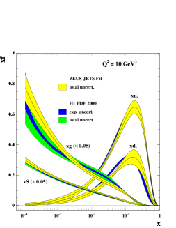
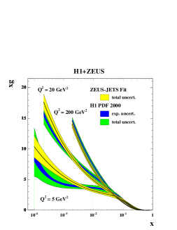
Fig. 1 compares the results of the H1 and ZEUS analyses. Whereas the extracted PDFs are broadly compatible within errors, there is a noticeable difference in the shape of the gluon PDFs.

Figure 1: Left plot: Comparison of PDFs from ZEUS and H1 analyses at $Q^{2}=10$GeV². Right plot: Comparison of gluon from ZEUS and H1 analyses, at various $Q^{2}$. Note that the ZEUS analysis total uncertainty includes both experimental and model uncertainties.

Full details of the analyses are given in the relevant publications, in this contribution we examine the differences in the two analyses, recapping only salient details.

The kinematics of lepton hadron scattering is described in terms of the variables $Q^{2}$, the invariant mass of the exchanged vector boson, Bjorken $x$, the fraction of the momentum of the incoming nucleon taken by the struck quark (in the quark-parton model), and $y$ which measures the energy transfer between the lepton and hadron systems. The differential cross-section for the NC process is given in terms of the structure functions by

$$\frac{d^{2}\sigma(e^{\pm}p)}{dxdQ^{2}}=\frac{2\pi\alpha^{2}}{Q^{4}x}\left[Y_{+}\,F_{2}(x,Q^{2})-y^{2}\,F_{L}(x,Q^{2})\mp Y_{-}\,xF_{3}(x,Q^{2})\right],$$

where $\displaystyle Y_{\pm}=1\pm(1-y)^{2}$. The structure functions $F_{2}$ and $xF_{3}$ are directly related to quark distributions, and their $Q^{2}$ dependence, or scaling violation, is predicted by pQCD. At $Q^{2}\leq 1000$ GeV² $F_{2}$ dominates the charged lepton-hadron cross-section and for $x\leq 10^{-2}$, $F_{2}$ itself is sea quark dominated but its $Q^{2}$ evolution is controlled by the gluon contribution, such that HERA data provide crucial information on low-$x$ sea-quark and gluon distributions. At high $Q^{2}$, the structure function $xF_{3}$ becomes increasingly important, and gives information on valence quark distributions. The CC interactions enable us to separate the flavour of the valence distributions at high-$x$, since their (LO) cross-sections are given by,

$$\frac{d^{2}\sigma(e^{+}p)}{dxdQ^{2}}=\frac{G_{F}^{2}M_{W}^{4}}{(Q^{2}+M_{W}^{2})^{2}2\pi x}x\left[(\bar{u}+\bar{c})+(1-y)^{2}(d+s)\right],$$

$$\frac{d^{2}\sigma(e^{-}p)}{dxdQ^{2}}=\frac{G_{F}^{2}M_{W}^{4}}{(Q^{2}+M_{W}^{2})^{2}2\pi x}x\left[(u+c)+(1-y)^{2}(\bar{d}+\bar{s})\right].$$

For both HERA analyses the QCD predictions for the structure functions are obtained by solving the DGLAP evolution equations [6] at NLO in the $\overline{\rm{MS}}$ scheme with the renormalisation and factorization scales chosen to be $Q^{2}$. These equations yield the PDFs at all values of $Q^{2}$ provided they are input as functions of $x$ at some input scale $Q^{2}_{0}$. The resulting PDFs are then convoluted with coefficient functions, to give the structure functions which enter into the expressions for the cross-sections. For a full explanation of the relationships between DIS cross-sections, structure functions, PDFs and the QCD improved parton model see ref. [10].

The HERA data are all in a kinematic region where there is no sensitivity to target mass and higher twist contributions but a minimum $Q^{2}$ cut must be imposed to remain in the kinematic region where perturbative QCD should be applicable. For ZEUS this is $Q^{2}>2.5$ GeV², and for H1 it is $Q^{2}>3.5$ GeV². Both collaborations have included the sensitivity to this cut as part of their model errors.

In the ZEUS analysis, the PDFs for $u$ valence, $xu_{v}(x)$, $d$ valence, $xd_{v}(x)$, total sea, $xS(x)$, the gluon, $xg(x)$, and the difference between the $d$ and $u$ contributions to the sea, $x(\bar{d}-\bar{u})$, are each parametrized by the form

$$p_{1}x^{p_{2}}(1-x)^{p_{3}}P(x),$$ (1)

where $P(x)=1+p_{4}x$, at $Q^{2}_{0}=7$GeV². The total sea $xS=2x(\bar{u}+\bar{d}+\bar{s}+\bar{c}+\bar{b})$, where $\bar{q}=q_{sea}$ for each flavour, $u=u_{v}+u_{sea},d=d_{v}+d_{sea}$ and $q=q_{sea}$ for all other flavours. The flavour structure of the light quark sea allows for the violation of the Gottfried sum rule. However, there is no information on the shape of the $\bar{d}-\bar{u}$ distribution in a fit to HERA data alone and so this distribution has its shape fixed consistent with the Drell-Yan data and its normalisation consistent with the size of the Gottfried sum-rule violation. A suppression of the strange sea with respect to the non-strange sea of a factor of 2 at $Q^{2}_{0}$, is also imposed consistent with neutrino induced dimuon data from CCFR. Parameters are further restricted as follows. The normalisation parameters, $p_{1}$, for the $d$ and $u$ valence and for the gluon are constrained to impose the number sum-rules and momentum sum-rule. The $p_{2}$ parameter which constrains the low-$x$ behaviour of the $u$ and $d$ valence distributions is set equal, since there is no information to constrain any difference. When fitting to HERA data alone it is also necessary to constrain the high-$x$ sea and gluon shapes, because HERA-I data do not have high statistics at large-$x$, in the region where these distributions are small. The sea shape has been restricted by setting $p_{4}=0$ for the sea, but the gluon shape is constrained by including data on jet production in the PDF fit. Finally the ZEUS analysis has 11 free PDF parameters. ZEUS have included reasonable variations of these assumptions about the input parametrization in their analysis of model uncertainties. The strong coupling constant was fixed to $\alpha_{s}(M_{Z}^{2})=0.118$ [11]. Full account has been taken of correlated experimental systematic errors by the Offset Method, as described in ref [3, 12].

For the H1 analysis, the value of $Q^{2}_{0}=4$GeV², and the choice of quark distributions which are parametrized is different. The quarks are considered as $u$-type and $d$-type with different parametrizations for, $xU=x(u_{v}+u_{sea}+c)$, $xD=x(d_{v}+d_{sea}+s)$, $x\bar{U}=x(\bar{u}+\bar{c})$ and $x\bar{D}=x(\bar{d}+\bar{s})$, with $q_{sea}=\bar{q}$, as usual, and the the form of the quark and gluon parametrizations given by Eq. 1. For $x\bar{D}$ and $x\bar{U}$ the polynomial, $P(x)=1.0$, for the gluon and $xD$, $P(x)=(1+p_{4}x)$, and for $xU$, $P(x)=(1+p_{4}x+p_{5}x^{3})$. The parametrization is then further restricted as follows. Since the valence distributions must vanish as $x\to 0$, the low-$x$ parameters, $p_{1}$ and $p_{2}$ are set equal for $xU$ and $x\bar{U}$, and for $xD$ and $x\bar{D}$. Since there is no information on the flavour structure of the sea it is also necessary to set $p_{2}$ equal for $x\bar{U}$ and $x\bar{D}$. The normalisation, $p_{1}$, of the gluon is determined from the momentum sum-rule and the $p_{4}$ parameters for $xU$ and $xD$ are determined from the valence number sum-rules. Assuming that the strange and charm quark distributions can be expressed as $x$ independent fractions, $f_{s}$ and $f_{c}$, of the $d$ and $u$ type sea, gives the further constraint $p_{1}(\bar{U})=p_{1}(\bar{D})(1-f_{s})/(1-f_{c})$. Finally there are 10 free parameters. H1 have also included reasonable variations of these assumptions in their analysis of model uncertainties. The strong coupling constant was fixed to $\alpha_{s}(M_{Z}^{2})=0.1185$ and this is sufficiently similar to the ZEUS choice that we can rule it out as a cause of any significant difference. Full account has been taken of correlated experimental systematic errors by the Hessian Method, see ref. [12].

For the ZEUS analysis, the heavy quark production scheme used is the general mass variable flavour number scheme of Roberts and Thorne [13]. For the H1 analysis, the zero mass variable flavour number scheme is used. It is well known that these choices have a small effect on the steepness of the gluon at very small-$x$, such that the zero-mass choice produces a slightly less steep gluon. However, there is no effect on the more striking differences in the gluon shapes at larger $x$.

There are two differences in the analyses which are worth further investigation. The different choices for the form of the PDF parametrization at $Q^{2}_{0}$ and the different treatment of the correlated experimental uncertainties.

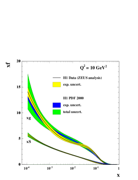
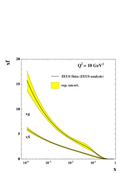
So far we have compared the results of putting two different data sets into two different analyses. Because there are many differences in the assumptions going into these analyses it is instructive to consider:(i) putting both data sets through the same analysis and (ii) putting one of the data sets through both analyses. For these comparisons, the ZEUS analysis does NOT include the jet data, so that the data sets are more directly comparable, involving just the inclusive double differential cross-section data. Fig. 2 compares the sea and gluon PDFs, at $Q^{2}=10$GeV², extracted from H1 data using the H1 PDF analysis with those extracted from H1 data using the ZEUS PDF analysis. These alternative analyses of the same data set give results which are compatible within the model dependence error bands. Fig. 2 also compares the sea and gluon PDFs extracted from ZEUS data using the ZEUS analysis with those extracted from H1 data using the ZEUS analysis. From this comparison we can see that the different data sets lead to somewhat different gluon shapes even when put through exactly the same analysis. Hence the most of the difference in shape of the ZEUS and H1 PDF analyses can be traced back to a difference at the level of the data sets.

Figure 2: Sea and gluon distributions at $Q^{2}=10$GeV² extracted from different data sets and different analyses. Left plot: H1 data put through both ZEUS and H1 analyses. Middle plot: ZEUS data put through ZEUS analysis. Right plot: H1 data put through ZEUS analysis.

Before going further it is useful to discuss the treatment of correlated systematic errors in the ZEUS and H1 analyses. A full discussion of the treatment of correlated systematic errors in PDF analyses is given in ref [10], only salient details are recapped here. Traditionally, experimental collaborations have evaluated an overall systematic uncertainty on each data point and these have been treated as uncorrelated, such that they are simply added to the statistical uncertainties in quadrature when evaluating $\chi^{2}$. However, modern deep inelastic scattering experiments have very small statistical uncertainties, so that the contribution of systematic uncertainties becomes dominant and consideration of point to point correlations between systematic uncertainties is essential.

For both ZEUS and H1 analyses the formulation of the $\chi^{2}$ including correlated systematic uncertainties is constructed as follows. The correlated uncertainties are included in the theoretical prediction, $F_{i}(p,s)$, such that

$$F_{i}(p,s)=F_{i}^{\rm NLOQCD}(p)+\sum_{\lambda}s_{\lambda}\Delta^{\rm sys}_{i\lambda}$$

where, $F_{i}^{\rm NLOQCD}(p)$, represents the prediction from NLO QCD in terms of the theoretical parameters $p$, and the parameters $s_{\lambda}$ represent independent variables for each source of systematic uncertainty. They have zero mean and unit variance by construction. The symbol $\Delta^{\rm sys}_{i\lambda}$ represents the one standard deviation correlated systematic error on data point $i$ due to correlated error source $\lambda$. The $\chi^{2}$ is then formulated as

$$\chi^{2}=\sum_{i}\frac{\left[F_{i}(p,s)-F_{i}(\rm meas)\right]^{2}}{\sigma_{i}^{2}}+\sum_{\lambda}s^{2}_{\lambda}$$ (2)

where, $F_{i}(\rm meas)$, represents a measured data point and the symbol $\sigma_{i}$ represents the one standard deviation uncorrelated error on data point $i$, from both statistical and systematic sources. The experiments use this $\chi^{2}$ in different ways. ZEUS uses the Offset method and H1 uses the Hessian method.

Traditionally, experimentalists have used ‘Offset’ methods to account for correlated systematic errors. The $\chi^{2}$ is formluated without any terms due to correlated systematic errors ($s_{\lambda}=0$ in Eq. 2) for evaluation of the central values of the fit parameters. However, the data points are then offset to account for each source of systematic error in turn (i.e. set $s_{\lambda}=+1$ and then $s_{\lambda}=-1$ for each source $\lambda$) and a new fit is performed for each of these variations. The resulting deviations of the theoretical parameters from their central values are added in quadrature. (Positive and negative deviations are added in quadrature separately.) This method does not assume that the systematic uncertainties are Gaussian distributed. An equivalent (and much more efficient) procedure to perform the Offset method has been given by Pascaud and Zomer [14], and this is what is actually used. The Offset method is a conservative method of error estimation as compared to the Hessian method. It gives fitted theoretical predictions which are as close as possible to the central values of the published data. It does not use the full statistical power of the fit to improve the estimates of $s_{\lambda}$, since it choses to mistrust the systematic error estimates, but it is correspondingly more robust.

The Hessian method is an alternative procedure in which the systematic uncertainty parameters $s_{\lambda}$ are allowed to vary in the main fit when determining the values of the theoretical parameters. Effectively, the theoretical prediction is not fitted to the central values of the published experimental data, but these data points are allowed to move collectively, according to their correlated systematic uncertainties. The theoretical prediction determines the optimal settings for correlated systematic shifts of experimental data points such that the most consistent fit to all data sets is obtained. Thus, in a global fit, systematic shifts in one experiment are correlated to those in another experiment by the fit. In essence one is allowing the theory to calibrate the detectors. This requires great confidence in the theory, but more significantly, it requires confidence in the many model choices which go into setting the boundary conditions for the theory (such as the parametrization at $Q^{2}_{0}$).

The ZEUS analysis can be performed using the Hessian method as well as the Offset method and Fig. 3 compares the PDFs, and their uncertainties, extracted from ZEUS data using these two methods.

Figure 3: PDFs at $Q^{2}=10$GeV², for the ZEUS analysis of ZEUS data performed by the Offset and the Hessian methods.

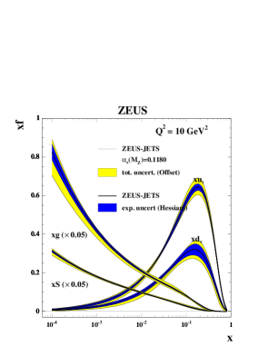
The central values of the different methods are in good agreement but the use of the Hessian method results in smaller uncertainties, for a the standard set of model assumptions, since the input data can be shifted within their correlated systematic uncertainties to suit the theory better. However, model uncertainties are more significant for the Hessian method than for the Offset method. The experimental uncertainty band for any one set of model choices is set by the usual $\chi^{2}$ tolerance, $\Delta\chi^{2}=1$, but the acceptability of a different set of choices is judged by the hypothesis testing criterion, such that the $\chi^{2}$ should be approximately in the range $N\pm\surd(2N)$, where $N$ is the number of degrees of freedom. The PDF parameters obtained for the different model choices can differ by much more than their experimental uncertainties, because each model choice can result in somewhat different values of the systematic uncertainty parameters, $s_{\lambda}$, and thus a different estimate of the shifted positions of the data points. This results in a larger spread of model uncertainty than in the Offset method, for which the data points cannot move. Fig 1 illustrates the comparability of the ZEUS (Offset) total uncertainty estimate to the H1 (Hessian) experimental plus model uncertainty estimate.

Another issue which arises in relation to the Hessian method is that the data points should not be shifted far outside their one standard deviation systematic uncertainties. This can indicate inconsistencies between data sets, or parts of data sets, with respect to the rest of the data. The CTEQ collaboration have considered data inconsistencies in their most recent global fit [2]. They use the Hessian method but they increase the resulting uncertainty estimates, by increasing the $\chi^{2}$ tolerance to $\Delta\chi^{2}=100$, to allow for both model uncertainties and data inconsistencies. In setting this tolerance they have considered the distances from the $\chi^{2}$-minima of individual data sets to the global minimum for all data sets. These distances by far exceed the range allowed by the $\Delta\chi^{2}=1$ criterion. Strictly speaking such variations can indicate that data sets are inconsistent but the CTEQ collaboration take the view that all of the current world data sets must be considered acceptable and compatible at some level, even if strict statistical criteria are not met, since the conditions for the application of strict criteria, namely Gaussian error distributions, are also not met. It is not possible to simply drop “inconsistent” data sets, as then the partons in some regions would lose important constraints. On the other hand the level of “inconsistency” should be reflected in the uncertainties of the PDFs. This is achieved by raising the $\chi^{2}$ tolerance. This results in uncertainty estimates which are comparable to those achieved by using the Offset method [12].

Using data from a single experiment avoids questions of data consistency, but to get the most information from HERA it is necessary to put ZEUS and H1 data sets into the same analysis together, and then questions of consistency arise. Fig 4 compares the sea and gluon PDFs and the $u$ and $d$ valence PDFs extracted from the ZEUS PDF analysis of ZEUS data alone, to those extracted from the ZEUS PDF analysis of both H1 and ZEUS data.

Figure 4: Top plots: Sea and gluon distributions at $Q^{2}=10$GeV² extracted from H1 and ZEUS data using the ZEUS analysis (left) compared to those extracted from ZEUS data alone using the ZEUS analysis (right). Bottom Plots: Valence distributions at $Q^{2}=10$GeV², extracted from H1 and ZEUS data using the ZEUS analysis (left) compared to those extracted from ZEUS data alone using the ZEUS analysis (right).

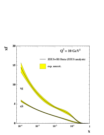
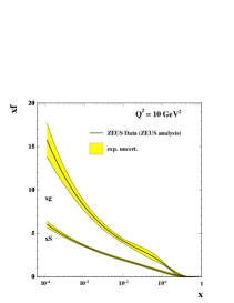
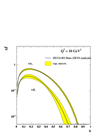
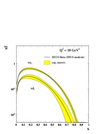
It is noticeable that, for the low-$x$ sea and gluon PDFs, combining the data sets does not bring a reduction in uncertainty equivalent to doubling the statistics. This is because the data which determine these PDFs are systematics limited. In fact there is some degree of tension between the ZEUS and the H1 data sets, such that the $\chi^{2}$ per degree of freedom rises for both data sets when they are fitted together. The Offset method of treating the systematic errors reflects this tension such that the overall uncertainty is not much improved when H1 data are added to ZEUS data. However, the uncertainty on the high-$x$ valence distributions is reduced by the input of H1 data, since the data are still statistics limited at high $x$.

Thus there could be an advantage in combining ZEUS and H1 data in a PDF fit if the tension between the data sets could be resolved. It is in this context the question of combining these data into a single data set arises. The procedure for combination is detailed in the contribution of S. Glazov to these proceedings. Essentially, since ZEUS and H1 are measuring the same physics in the same kinematic region, one can try to combine them using a ’theory-free’ Hessian fit in which the only assumption is that there is a true value of the cross-section, for each process, at each $x,Q^{2}$ point. The systematic uncertainty parameters, $s_{\lambda}$, of each experiment are fitted to determine the best fit to this assumption. Thus each experiment is calibrated to the other. This works well because the sources of systematic uncertainty in each experiment are rather different. Once the procedure has been performed the resulting systematic uncertainties on each of the combined data points are significantly smaller than the statistical errors. Thus one can legitimately make a fit to the combined data set in which these statistical and systematic uncertainties are simply combined in quadrature. The result of making such a fit, using the ZEUS analysis, is shown in Fig. 5.

Figure 5: Left plot: Sea and gluon distributions at $Q^{2}=10$GeV², extracted from the combined H1 and ZEUS data set using the ZEUS analysis. Right plot: Valence distributions at $Q^{2}=10$GeV², extracted from the combined H1 and ZEUS data set using the ZEUS analysis.

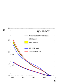
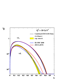
The central values of the ZEUS and H1 published analyses are also shown for comparison. Looking back to Fig. 4 one can see that there has been a dramatic reduction in the level of uncertainty compared to the ZEUS Offset method fit to the separate ZEUS and H1 data sets. This result is very promising. A preliminary study of model dependence, varying the form of the polynomial, $P(x)$, used in the PDF paremtrizations at $Q^{2}_{0}$, also indicates that model dependence is relatively small.

The tension between ZEUS and H1 data could have been resolved by putting them both into a PDF fit using the Hessian method to shift the data points. That is, rather than calibrating the two experiments to each other in the ’theory-free’ fit, we could have used the theory of pQCD to calibrate each experiment. Fig. 6 shows the PDFs extracted when the ZEUS and H1 data sets are put through the ZEUS PDF analysis procedure using the Hessian method.

Figure 6: Left plot: Sea and gluon distributions at $Q^{2}=10$GeV², extracted from the H1 and ZEUS data sets using the ZEUS analysis done by Hessian method. Right plot: Valence distributions at $Q^{2}=10$GeV², extracted from the H1 and ZEUS data sets using the ZEUS analysis done by Hessian method.

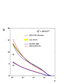
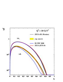
The uncertainties on the resulting PDFs are comparable to those found for the fit to the combined data set, see Fig. 5. However, the central values of the resulting PDFs are rather different- particularly for the less well known gluon and $d$ valence PDFs. For both of the fits shown in Figs. 5, 6 the values of the systematic error parameters, $s_{\lambda}$, for each experiment have been allowed to float so that the data points are shifted to give a better fit to our assumptions, but the values of the systematic error parameters chosen by the ’theory-free’ fit and by the PDF fit are rather different. A representaive sample of these values is given in Table 1. These discrepancies might be somewhat alleviated by a full consideration of model errors in the PDF fit, or of appropriate $\chi^{2}$ tolerance when combining the ZEUS and H1 experiments in a PDF fit, but these differences should make us wary about the uncritical use of the Hessian method.

Syatematic uncertainty $s_{\lambda}$	in PDF fit	in Theory-free fit
ZEUS electron efficiency	1.68	0.31
ZEUS electron angle	-1.26	-0.11
ZEUS electron energy scale	-1.04	0.97
ZEUS hadron calorimeter energy scale	1.05	-0.58
H1 electron energy scale	-0.51	0.61
H1 hadron energy scale	-0.26	-0.98
H1 calorimeter noise	1.00	-0.63
H1 photoproduction background	-0.36	0.97

Table 1: Systematic shifts for ZEUS and H1 data as determine by a joint pQCD PDF fit, and as determined by the theory-free data combination fit

References

- [1] A.D. Martin et al., Eur. Phys.J C23, 73 (2002)
- [2] J. Pumplin et al., JHEP 0207, 012 (2002)
- [3] ZEUS Coll., S. Chekanov et al., Phys. Rev D 67, 012007 (2003)
- [4] ZEUS Coll., S. Chekanov et al., Eur.Phys.J C 42, 1 (2005)
- [5] H1 Coll., C.Adloff et al., Eur.Phys.J C 30, 32 (2003)
- [6] G. Altarelli, G. Parisi, Nucl.Phys. B126, 298 (1977)
- [7] V.N. Gribov, L.N. Lipatov, Sov.J.Nucl.Phys 15, 438 (1972)
- [8] L.N. Lipatov, Sov.J.Nucl.Phys 20, 94 (1975)
- [9] Yu.L. Dokshitzer, JETP 46, 641 (1977)
- [10] R C E Devenish and A M Cooper-Sarkar, Deep Inelastic Scattering. Oxford Unviersity Press, Oxford, 2004
- [11] S. Eidelman, Phys.Lett B 592, 1 (2004)
- [12] A.M. Cooper-Sarkar, J.Phys G 28, 2669 (2002)
- [13] R.S. Thorne and R.G. Roberts, Phys.Rev D57, 6871 (1998)
- [14] C. Pascaud and F. Zomer, Correlated systematic error propagation. Preprint LAL-95-05, 1995.