CP Asymmetry, Branching ratios and Isospin breaking effects in $B\to\rho\gamma$ and $B\to\omega\gamma$ decays with the pQCD approach

Abstract

The radiative ${B\rightarrow\rho\gamma}$, ${B\to\omega\gamma}$ decay modes are caused by the flavor-changing-neutral-current process, so they give us good insight towards probing the standard model in order to search for new physics. In this paper, we compute the branching ratio, direct CP asymmetry, and isospin breaking effects using the perturbative QCD approach within the standard model.

1 Introduction

The standard model (SM) predicts large CP violation in ${B}$ decays [1, 2] and they have been verified in ${B\to J/\psi K_{s}}$ [3, 4], ${B\to\pi\pi}$ [5, 6], and ${B\to DK}$ [7] decays. The quest of high energy physics has always been to search for the most fundamental theory. So our immediate goal is to search for deviation from the predictions of the SM. It is believed that the quantum effects in ${B}$ meson decay amplitudes may contain effects of new physics.

The flavor-changing-neutral-current (FCNC) process which causes ${b\to s\gamma}$ and ${b\to d\gamma}$ decays may contain new physics (NP) effects through penguin amplitudes. As the SM effects represent the background when we search for NP effects, we shall compute these effects. In doing so, we can understand the sensitivity of each NP search.

The first experimental evidence of this FCNC transition process in ${B}$ decay was observed about a decade ago, where the inclusive process $b\to s\gamma$ and exclusive process $B\to K^{*}\gamma$ were detected, and their branching ratios were measured [8]. On the other hand, the expected branching ratio for ${b\to d\gamma}$ is suppressed by ${O(10^{-2})}$ with respect to that for ${b\to s\gamma}$, because of the Cabbibo-Kobayashi-Maskawa (CKM) quark-mixing matrix factor. The world average for ${b\to d}$ penguin decays is given as follows [9]:

$$\begin{cases}&Br(B^{0}\to\rho^{0}\gamma)=(0.38\pm 0.18)\times 10^{-6}\\ &Br(B^{0}\to\omega\gamma)=(0.54^{+0.23}_{-0.21})\times 10^{-6}\\ &Br(B^{+}\to\rho^{+}\gamma)=(0.68^{+0.36}_{-0.31})\times 10^{-6}.\end{cases}$$

Theoretically, $B\to\rho\gamma$ and $B\to\omega\gamma$ are widely studied both within and beyond the SM [10, 11]. The bound states are involved in the exclusive process, so the perturbation theory can not be used in a simple manner. It has been shown that, at least in the leading order, all nonperturbative effects can be included in the definition of the ${B}$ meson and the vector meson wave functions, and the rest of the amplitude (the hard part of the amplitude) can be computed in the perturbation theory. This is called the perturbative QCD (pQCD) approach and it was proven several years ago [12, 13]. In this paper, we compute the branching ratio, direct CP asymmetry, and isospin breaking effects for ${B\to\rho\gamma}$, ${B\to\omega\gamma}$ decays by using the pQCD within the SM.

The remaining part of this paper is organized as follows. In Sec.2, we briefly review the pQCD approach, and in Sec.3, we present some basic formulas such as the effective Hamiltonian and kinetic conventions. In Sec.4, the hard amplitudes calculated in pQCD are given. Section 5 is devoted to numerical calculation and discussion. Finally, a brief summary is given in Sec.6.

2 Perturbative QCD Approach

In order to explain the pQCD approach, we want to suppose that a static ${B^{+}}$ meson decays into ${\rho^{+}}$ and ${\gamma}$ through the ${O_{7\gamma}}$ operator as in Fig.1.

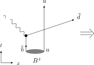
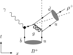
Figure 1: The heavy ${\bar{b}}$ quark decays into the light ${\bar{d}}$ quark and a photon through the electromagnetic operator, and the decay products dash away back-to-back with momenta ${O(M_{B}/2)}$. In order to form a ${\rho^{+}}$ meson with no hadron jets, the spectator quark must line up with ${\bar{d}}$. This can be accomplished most efficiently by exchanging a hard gluon

In the rest frame of the ${B^{+}}$ meson, the ${\bar{b}}$ quark is almost at rest and the spectator ${u}$ quark moves around the ${\bar{b}}$ quark with ${O(\Lambda)=O(M_{B}-m_{b})}$ momentum, where ${M_{B}}$, and ${m_{b}}$ are ${B}$ meson, and ${b}$ quark mass, respectively. Then the ${\bar{b}}$ quark decays into ${\bar{d}}$ and ${\gamma}$, and these products dash away back-to-back with ${O(M_{B}/2)}$ momenta. When a quark is rapidly accelerated like this, infinitely many gluons are likely to be emitted by bremsstrahlung. There is a familiar phenomena in QED, when an electrically charged particle is accelerated, infinitely many photons are emitted. But the gluon emission by bremsstrahlung QCD must result in many hadrons in the final state. As the emitted gluon will hadronize, the fact that no hadron except for ${\rho(\omega)}$ should be observed in ${B\to\rho(\omega)\gamma}$, means that the bremsstrahlung gluon emission mentioned above can not occur. Thus the branching ratio for an exclusive decay ${B\to\rho(\omega)\gamma}$ is proportional to the probability that no bremsstrahlung gluon is emitted. The amplitude for an exclusive decay contains the Sudakov factor and it is depicted in Fig.2. As seen in Fig.2, the Sudakov factor is large for small ${b}$ and small ${Q}$, where ${b}$ is the spacial distance between quark and antiquark into ${B}$ meson, as shown in Fig.3, and ${Q}$ is the ${b}$ quark momentum inside the ${B}$ meson. Large ${b}$ implies that the quark and antiquark pair is separated in space, which in turn implies less color shielding. Similar absence of the color shielding occurs when the ${b}$ quark carries the most of the momentum of the ${B}$ meson. That is, as seen in Fig.2, in order to form a ${\rho(\omega)}$ meson with no hadron jets, the condition for color shielding is essential. The condition needed for the color shielding is the small separation in space between quark and antiquark within the meson, and it indicates that the energy scale of the decay process should be high. Actually, the invariant-mass square of the exchanged gluon depicted in Fig.1 is about ${O(\Lambda M_{B})}$, which can be considered to be in the short distance regime. Thus we can see that the decay process can be treated perturbatively. The decay amplitude for the exclusive mode like ${B\to\rho(\omega)\gamma}$ decay can be factorized into the hard part with a hard gluon exchange, which can be treated perturbatively, and the soft part of all nonperturbative strong interactions is included in the meson wave functions.

Figure 2: The dependence of the Sudakov factor ${\exp[-s(Q,b)]}$ on ${Q}$ and ${b}$ where ${Q}$ is the ${b}$ quark momentum, and ${b}$ is the interval between quarks which form hadrons. It is clear that the large ${b}$ and ${Q}$ region is suppressed.

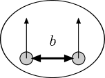
Figure 3: ${b}$ is the transverse interval between the ${\bar{b}}$ and ${u}$ quark in the ${B}$ meson.

Then the total decay amplitude can be expressed as the convolution like

$$\int^{1}_{0}dx_{1}dx_{2}\int^{1/\Lambda}_{0}d^{2}b_{1}d^{2}b_{2}\hskip 2.84526ptC(t)\otimes\exp{[-S(x_{1},x_{2},b_{1},b_{2},t)]}$$

$$\hskip 71.13188pt\otimes\Phi_{\rho,\hskip 2.84526pt\omega}(x_{2},b_{2})\hskip 2.84526pt\otimes H(x_{1},x_{2},b_{1},b_{2},t)\otimes\Phi_{B}(x_{1},b_{1}),$$ (1)

where ${\Phi_{\rho\hskip 2.84526pt\omega}(x_{2},b_{2})}$ and ${\Phi_{B}(x_{1},b_{1})}$ are meson distribution amplitudes, ${\exp{[-S(x_{1},x_{2},b_{1},b_{2},t)]}}$ is the Sudakov factor, which results from summing up all the double logarithms of the soft divergences. ${H(x_{1},x_{2},b_{1},b_{2},t)}$ is the hard kernel including finite piece of quantum correction, ${b_{1}}$, ${b_{2}}$ are the conjugate variables to transverse momenta, and ${x_{1}}$, ${x_{2}}$ are the momentum fractions of spectator quarks.

In the computation of the decay amplitudes with the pQCD approach, we adopt the model functions for the meson distribution amplitudes. The meson amplitudes are characterized by the strong interaction. The effective range of the strong interaction which can propagate, is wide. Then the meson distribution amplitudes should be expressed as some averaged physical quantity. Thus the meson amplitude does not depend on the decay process etc. For the ${B}$ meson wave function, we adopt a model [14]. For the ${\rho}$ and ${\omega}$ meson wave function, we use ones determined by the light-cone QCD sum rule [15]. The detailed expressions for the meson functions are in Appendix A.

3 Basic formulas

The flavor-changing ${b\rightarrow d\gamma}$ transition induced by an effective Hamiltonian is given by [16]

$$H_{\mbox{\scriptsize{eff}}} = \frac{G_{F}}{\sqrt{2}}\Big{[}V_{ub}V_{ud}^{*}\left\{C_{1}^{(u)}(\mu)O_{1}^{(u)}(\mu)+C_{2}^{(u)}(\mu)O_{2}^{(u)}(\mu)\right\}$$

$$\hskip 17.07164pt+V_{cb}V_{cd}^{*}\left\{C_{1}^{(c)}(\mu)O_{1}^{(c)}(\mu)+C_{2}^{(c)}(\mu)O_{2}^{(c)}(\mu)\right\}$$

$$\hskip 17.07164pt-V_{tb}V_{td}^{*}\Big{\{}\sum_{i=3\sim 6}C_{i}(\mu)O_{i}(\mu)+C_{7\gamma}(\mu)O_{7\gamma}(\mu)+C_{8g}(\mu)O_{8g}(\mu)\Big{\}}\Big{]}+(\mbox{h.c.}),$$

where $C_{i}$’s are Wilson coefficients, and $O_{i}$’s are local operators which are given by

$$O_{1}^{(q)} = (\bar{d}_{i}q_{j})_{V-A}(\bar{q}_{j}b_{i})_{V-A},\hskip 73.97733ptO_{2}^{(q)}=(\bar{d}_{i}q_{i})_{V-A}(\bar{q}_{j}b_{j})_{V-A},$$

$$O_{3}^{(q)} = (\bar{d}_{i}b_{i})_{V-A}\sum_{q}(\bar{q}_{j}q_{j})_{V-A},\hskip 56.9055ptO_{4}^{(q)}=(\bar{d}_{i}b_{j})_{V-A}\sum_{q}(\bar{q}_{j}q_{i})_{V-A},$$

$$O_{5}^{(q)} = (\bar{d}_{i}b_{i})_{V-A}\sum_{q}(\bar{q}_{j}q_{j})_{V+A},\hskip 56.9055ptO_{6}^{(q)}=(\bar{d}_{i}b_{j})_{V-A}\sum_{q}(\bar{q}_{j}q_{i})_{V+A},$$ (3)

$$O_{7\gamma} = \frac{e}{8{\pi}^{2}}m_{b}\bar{d}_{i}\sigma^{\mu\nu}(1+\gamma_{5})b_{i}F_{\mu\nu},\hskip 45.5244ptO_{8g}=\frac{g}{8{\pi}^{2}}m_{b}\bar{d}_{i}\sigma^{\mu\nu}(1+\gamma_{5})T_{ij}^{a}b_{j}G_{\mu\nu}^{a},$$

and we neglect the terms which are proportional to ${d}$ quark mass in ${O_{7\gamma}}$ and ${O_{8g}}$. Here ${(\bar{q}_{i}q_{j})_{V\mp A}}$ means ${\bar{q}_{i}\gamma^{\mu}(1\mp\gamma^{5})q_{j}}$, and ${i}$, ${j}$ are color indexes. With the effective Hamiltonian given above, the decay amplitude of $B\to\rho(\omega)\gamma$ can be expressed as

$$A=\langle F|H_{\mbox{\scriptsize{eff}}}|B\rangle=\frac{G_{F}}{\sqrt{2}}\sum_{i,q}V_{qb}^{*}V_{qd}C_{i}(\mu)\langle F|O_{i}(\mu)|B\rangle,$$ (4)

where $F$ denotes the final state $\rho\gamma$ or $\omega\gamma$. In addition, the amplitude can be decomposed into scalar (${M^{S}}$) and pseudo-scalar (${M^{P}}$) components as

$$A=(\varepsilon_{V}^{*}\cdot\varepsilon_{\gamma}^{*})M^{S}+\frac{i}{P_{V}\cdot P_{\gamma}}\epsilon_{\mu\nu\rho\sigma}\varepsilon_{\gamma}^{*\mu}\varepsilon_{V}^{*\nu}P_{\gamma}^{\rho}P_{V}^{\sigma}M^{P},$$ (5)

where $P_{V}$, and $P_{\gamma}$ are the momenta of $\rho$($\omega$) meson, and photon, respectively. $\varepsilon_{\gamma}^{*}$ and $\varepsilon_{V}^{*}$ are the relevant polarization vectors. The matrix element $\langle F|O_{i}(\mu)|B\rangle$ can be calculated in the pQCD approach.

For convenience, we work in light-cone coordinate. Then the momentum is taken in the form

$$p=(p^{+},p^{-},\vec{p}_{T})=\left(\frac{p^{0}+p^{3}}{\sqrt{2}},\frac{p^{0}-p^{3}}{\sqrt{2}},(p^{1},p^{2})\right),$$ (6)

and the scalar product of two arbitrary vectors $A$ and $B$ is $A\cdot B=A_{\mu}B^{\mu}=(A^{+}B^{-}+A^{-}B^{+})-\vec{A}_{\bot}\cdot\vec{B}_{\bot}$. In the $B$ meson rest frame, the momentum of $B$ meson is

$$P_{B}=(P_{B}^{+},P_{B}^{-},\vec{P}_{B\perp})=\frac{M_{B}}{\sqrt{2}}(1,1,\vec{0}_{\bot}),$$ (7)

and by choosing the coordinate frame where the $\rho$ or $\omega$ meson moves in the “-” and photon in the “+” direction, the momenta of final state particles are

$$P_{\gamma} = (P_{\gamma}^{+},P_{\gamma}^{-},\vec{P}_{\gamma\perp})=\frac{M_{B}}{\sqrt{2}}(1,0,\vec{0}_{\bot}),$$ (8)

$$P_{V} = (P_{V}^{+},P_{V}^{-},\vec{P}_{V\perp})=\frac{M_{B}}{\sqrt{2}}(0,1,\vec{0}_{\bot}).$$ (9)

The momenta of the spectator quarks in $B$ and $\rho$ or $\omega$ mesons are

$$k_{1} = (k_{1}^{+},k_{1}^{-},\vec{k}_{1T})=(\frac{M_{B}}{\sqrt{2}}x_{1},0,\vec{k_{1T}}),$$ (10)

$$k_{2} = (k_{2}^{+},k_{2}^{-},\vec{k}_{2T})=(0,\frac{M_{B}}{\sqrt{2}}x_{2},\vec{k_{2T}}),$$ (11)

where $x_{1}$, and $x_{2}$ are momentum fractions which are defined by $x_{1}=k_{1}^{+}/P_{B}^{+}$, and $x_{2}=k_{2}^{-}/P_{V}^{-}$, respectively.

4 Formulas of the hard amplitude

In this section we give the amplitudes caused by each operator in Eq.(3).

4.1 Contribution of $O_{7\gamma}$

Figure 4: Contribution from operator $O_{7\gamma}$ to $B\to\rho(\omega)\gamma$ decay. The photon is emitted through the operator, and hard gluon exchange is need to form a ${\rho(\omega)}$ meson.

At first, we present the contribution of the electromagnetic operator $O_{7\gamma}$. The diagrams are shown in Fig.4. In this case, the photon is emitted through the operator, and hard gluon exchange is needed to form a ${\rho(\omega)}$ meson. Contributions of the $O_{7\gamma}$ operator to the amplitudes $M^{S}$ and $M^{P}$ defined in Eq.(5) are as follows:

$$M_{7\gamma}^{S(a)} = -M_{7\gamma}^{P(a)}$$ (12)

$$= -2F^{(0)}\xi_{t}\int dx_{1}dx_{2}\int db_{1}db_{2}b_{1}b_{2}\alpha_{s}(t_{7}^{a})\exp[-S_{B}(t_{7}^{a})-S_{V}(t_{7}^{a})]S_{t}(x_{1})C_{7\gamma}(t_{7}^{a})\phi_{B}(x_{1},b_{1})$$

$$\times r_{V}\Big{[}\phi^{v}_{V}(x_{2})+\phi^{a}_{V}(x_{2})\Big{]}H_{7}^{(a)}(A_{7}b_{2},B_{7}b_{1},B_{7}b_{2}),$$

$$\hskip 85.35826pt\left(t_{7}^{a}=\mbox{max}(A_{7},B_{7},1/b_{1},1/b_{2})\right),$$

$$M_{7\gamma}^{S(b)} = -M_{7\gamma}^{P(b)}$$ (13)

$$= -2F^{(0)}\xi_{t}\int dx_{1}dx_{2}\int db_{1}db_{2}b_{1}b_{2}\alpha_{s}(t_{7}^{b})\exp[-S_{B}(t_{7}^{b})-S_{V}(t_{7}^{b})]S_{t}(x_{2})C_{7\gamma}(t_{7}^{b})\phi_{B}(x_{1},b_{1})$$

$$\times \Big{[}(1+x_{2})\phi^{T}_{V}(x_{2})+(1-2x_{2})r_{V}[\phi^{a}_{V}(x_{2})+\phi^{v}_{V}(x_{2})]\Big{]}H_{7}^{(b)}(A_{7}b_{1},C_{7}b_{1},C_{7}b_{2}),$$

$$\hskip 85.35826pt\left(t_{7}^{b}=\mbox{max}(A_{7},C_{7},1/b_{1},1/b_{2})\right),$$

$$H_{7}^{(a)}\left(A_{7}b_{2},B_{7}b_{1},B_{7}b_{2}\right) \equiv K_{0}(A_{7}b_{2})\Big{[}\theta(b_{1}-b_{2})K_{0}\left(B_{7}b_{1}\right)I_{0}\left(B_{7}b_{2}\right)$$ (14)

$$\hskip 85.35826pt+\theta(b_{2}-b_{1})K_{0}\left(B_{7}b_{2}\right)I_{0}\left(B_{7}b_{1}\right)\Big{]},$$

$$H_{7}^{(b)}(A_{7}b_{1},C_{7}b_{1},C_{7}b_{2})=H_{7}^{(a)}(A_{7}b_{1},C_{7}b_{1},C_{7}b_{2}),$$ (15)

$$A_{7}^{2}=x_{1}x_{2}M_{B}^{2},\hskip 14.22636ptB_{7}^{2}=x_{1}{M_{B}}^{2},\hskip 14.22636ptC_{7}^{2}=x_{2}M_{B}^{2}.$$ (16)

Here ${K_{0},~{}I_{0}}$ are modified Bessel functions which are extracted by the propagator integrations. We define the common factor as

$$F^{(0)}=\frac{G_{F}}{\sqrt{2}}\frac{e}{\pi}C_{F}M_{B}^{5},$$ (17)

and the CKM matrix element as ${\xi_{q}=V_{qb}^{*}V_{qs}}$. The exponentials $\exp[-S_{B}(t)]$ and $\exp[-S_{V}(t)]$ are the Sudakov factors [12], and the explicit expressions of the exponents $S_{B}$, $S_{V}$ are shown in Appendix B. The quark structures for vector mesons are ${\rho^{+}=|\bar{d}u\rangle}$,  ${\rho^{0}=|\bar{u}u-\bar{d}d\rangle/\sqrt{2}}$,  and ${\omega=|\bar{u}u+\bar{d}d\rangle/\sqrt{2}}$, then the decay amplitudes for each decay modes caused by ${O_{7\gamma}}$ operator are given as follows:

$$M(B^{+}\to\rho^{+}\gamma)_{7\gamma}^{j} = M_{7\gamma}^{j(a)}+M_{7\gamma}^{j(b)},$$ (18)

$$M(B^{0}\to\rho^{0}\gamma)_{7\gamma}^{j} = -\frac{1}{\sqrt{2}}\left[M_{7\gamma}^{j(a)}+M_{7\gamma}^{j(b)}\right],$$ (19)

$$M(B^{0}\to\omega\gamma)_{7\gamma}^{j} = \frac{1}{\sqrt{2}}\left[M_{7\gamma}^{j(a)}+M_{7\gamma}^{j(b)}\right],$$ (20)

where ${j}$ expresses the decay amplitude components ${S}$ or ${P}$.

4.2 Contribution of $O_{8g}$

Figure 5: Diagrams for the contribution of the chromomagnetic operator $O_{8g}$. A hard gluon is emitted through the $O_{8g}$ operator and glued to the spectator quark line. Thus a photon is emitted by the bremsstrahlung of the external quark lines.

The diagrams for the contribution of the chromomagnetic penguin operator $O_{8g}$ are shown in Fig.5. Contributions of each diagram are given in the following. In this case, a hard gluon is emitted through the ${O_{8g}}$ operator and glued to the spectator quark line, and a photon is emitted by the bremsstrahlung from the external quark lines. Each decay amplitude caused by ${O_{8g}}$ operator is expressed as follows:

$$M_{8}^{S(a)}(Q_{b}) = -M_{8}^{P(a)}(Q_{b})$$ (21)

$$= -F^{(0)}\xi_{t}Q_{b}\int dx_{1}dx_{2}\int db_{1}db_{2}b_{1}b_{2}\alpha_{s}(t_{8}^{a})\exp[-S_{B}(t_{8}^{a})-S_{V}(t_{8}^{a})]S_{t}(x_{1})$$

$$\times C_{8g}(t_{8}^{a})\phi_{B}(x_{1},b_{1})\left[x_{2}r_{V}\phi^{a}_{V}(x_{2})+x_{1}\phi^{T}_{V}(x_{2})+x_{2}r_{V}\phi^{v}_{V}(x_{2})\right]$$

$$\times H_{8}^{(a)}(A_{8}b_{2},B_{8}b_{1},B_{8}b_{2}),$$

$$\hskip 56.9055pt\left(t_{8}^{a}=\mbox{max}(A_{8},B_{8},1/b_{1},1/b_{2})\right),$$

$$M_{8}^{S(b)}(Q_{d}) = -M_{8}^{P(b)}(Q_{d})$$ (22)

$$= -F^{(0)}\xi_{t}Q_{d}\int dx_{1}dx_{2}\int db_{1}db_{2}b_{1}b_{2}\alpha_{s}(t_{8}^{b})\exp[-S_{B}(t_{8}^{b})-S_{V}(t_{8}^{b})]S_{t}(x_{2})$$

$$\times C_{8g}(t_{8}^{b})\phi_{B}(x_{1},b_{1})\left[-3x_{2}r_{V}\phi^{a}_{V}(x_{2})+(2x_{2}-x_{1})\phi^{T}_{V}(x_{2})-3x_{2}r_{V}\phi^{v}_{V}(x_{2})\right]$$

$$\times H_{8}^{(b)}(A_{8}b_{1},C_{8}b_{1},C_{8}b_{2}),$$

$$\hskip 56.9055pt\left(t_{8}^{b}=\mbox{max}(A_{8},C_{8},1/b_{1},1/b_{2})\right),$$

$$M_{8}^{S(c)}(Q_{q}) = -M_{8}^{P(c)}(Q_{q})$$ (23)

$$= -F^{(0)}\xi_{t}Q_{q}\int dx_{1}dx_{2}\int db_{1}db_{2}b_{1}b_{2}\alpha_{s}(t_{8}^{c})\exp[-S_{B}(t_{8}^{c})-S_{V}(t_{8}^{c})]S_{t}(x_{1})$$

$$\times C_{8g}(t_{8}^{c})\phi_{B}(x_{1},b_{1})\left[x_{2}r_{V}\phi^{a}_{V}(x_{2})-x_{1}\phi^{T}_{V}(x_{2})+x_{2}r_{V}\phi^{v}_{V}(x_{2})\right]$$

$$\times H_{8}^{(c)}\left(\sqrt{|A_{8}^{{}^{\prime}2}|}b_{2},D_{8}b_{1},D_{8}b_{2}\right),$$

$$\hskip 56.9055pt\left(t_{8}^{c}=\mbox{max}(\sqrt{|A_{8}^{{}^{\prime}2}|},D_{8},1/b_{1},1/b_{2})\right),$$

$$M_{8}^{S(d)}(Q_{q}) = -F^{(0)}\xi_{t}Q_{q}\int dx_{1}dx_{2}\int db_{1}db_{2}b_{1}b_{2}\alpha_{s}(t_{8}^{d})\exp[-S_{B}(t_{8}^{d})-S_{V}(t_{8}^{d})]S_{t}(x_{2})$$ (24)

$$\times C_{8g}(t_{8}^{d})\phi_{B}(x_{1},b_{1})\left[(x_{2}-x_{1}+2)\phi^{T}_{V}(x_{2})+6x_{2}r_{V}\phi^{v}_{V}(x_{2})\right]$$

$$\times H_{8}^{(d)}\left(\sqrt{|A_{8}^{{}^{\prime}2}|}b_{1},E_{8}b_{1},E_{8}b_{2}\right),$$

$$M_{8}^{P(d)}(Q_{q}) = F^{(0)}\xi_{t}Q_{q}\int dx_{1}dx_{2}\int db_{1}db_{2}b_{1}b_{2}\alpha_{s}(t_{8}^{d})\exp[-S_{B}(t_{8}^{d})-S_{V}(t_{8}^{d})]S_{t}(x_{2})$$ (25)

$$\times C_{8g}(t_{8}^{d})\phi_{B}(x_{1},b_{1})\left[(x_{2}-x_{1}+2)\phi^{T}_{V}(x_{2})+6x_{2}r_{V}\phi^{a}_{V}(x_{2})\right]$$

$$\times H_{8}^{(d)}\left(\sqrt{|A_{8}^{{}^{\prime}2}|}b_{1},E_{8}b_{1},E_{8}b_{2}\right),$$

$$\hskip 56.9055pt\left(t_{8}^{d}=\mbox{max}(\sqrt{|A_{8}^{{}^{\prime}2}|},E_{8},1/b_{1},1/b_{2})\right),$$

$$H_{8}^{(a)}(A_{8}b_{2},B_{8}b_{1},B_{8}b_{2}) \equiv K_{0}(A_{8}b_{2})\Big{[}\theta(b_{1}-b_{2})K_{0}(B_{8}b_{1})I_{0}(B_{8}b_{2})+(b_{1}\leftrightarrow b_{2})\Big{]},$$ (26)

$$H_{8}^{(b)}(A_{8}b_{1},C_{8}b_{1},C_{8}b_{2}) \equiv \frac{i\pi}{2}K_{0}(A_{8}b_{1})\Big{[}\theta(b_{1}-b_{2})H_{0}^{(1)}(C_{8}b_{1})J_{0}(C_{8}b_{2})+(b_{1}\leftrightarrow b_{2})\Big{]},$$ (27)

$$H_{8}^{(c)}(\sqrt{|A_{8}^{\prime 2}|}b_{2},D_{8}b_{1},D_{8}b_{2}) \equiv \theta(A_{8}^{\prime 2})\hskip 2.84526ptK_{0}(\sqrt{|A_{8}^{\prime 2}|}b_{2})\Big{[}\theta(b_{1}-b_{2})K_{0}(D_{8}b_{1})I_{0}(D_{8}b_{2})+(b_{1}\leftrightarrow b_{2})\Big{]}$$ (28)

$$+\theta(-A_{8}^{\prime 2})\hskip 2.84526pti\frac{\pi}{2}H_{0}^{(1)}(\sqrt{|A_{8}^{\prime 2}|}b_{2})\Big{[}\theta(b_{1}-b_{2})K_{0}(D_{8}b_{1})I_{0}(D_{8}b_{2})+(b_{1}\leftrightarrow b_{2})\Big{]},\hskip 28.45274pt$$

$$H_{8}^{(d)}(\sqrt{|A_{8}^{\prime 2}|}b_{1},E_{8}b_{1},E_{8}b_{2}) \equiv \theta(A_{8}^{\prime 2})\hskip 2.84526pti\frac{\pi}{2}K_{0}(\sqrt{|A_{8}^{\prime 2}|}b_{1})\left[\theta(b_{1}-b_{2})H_{0}^{(1)}(E_{8}b_{1})J_{0}(E_{8}b_{2})+(b_{1}\leftrightarrow b_{2})\right]$$ (29)

$$-\theta(-A_{8}^{\prime 2})\hskip 2.84526pt\left(\frac{\pi}{2}\right)^{2}H_{0}^{(1)}(\sqrt{|A_{8}^{\prime 2}}|b_{1})\left[\theta(b_{1}-b_{2})H_{0}^{(1)}(E_{8}b_{1})J_{0}(E_{8}b_{2})+(b_{1}\leftrightarrow b_{2})\right],$$

$$A_{8}^{2} = x_{1}x_{2}M_{B}^{2},\hskip 22.76219ptB_{8}^{2}=M_{B}^{2}(1+x_{1}),\hskip 22.76219ptC_{8}^{2}=M_{B}^{2}(1-x_{2}),$$

$$A_{8}^{\prime 2} = (x_{1}-x_{2})M_{B}^{2},\hskip 22.76219ptD_{8}^{2}=x_{1}{M_{B}}^{2},\hskip 22.76219ptE_{8}^{2}=x_{2}{M_{B}}^{2}.$$ (30)

Here we define ${Q_{q}}$ as the electric charge for the quark ${q}$: ${Q_{b}=Q_{d}=-1/3}$ and ${Q_{u}=2/3}$. Then the decay amplitudes for each decay channels can be written as follows:

$$M(B^{+}\to\rho^{+}\gamma)_{8g}^{j} = M_{8g}^{j(a)}(Q_{b})+M_{8g}^{j(b)}(Q_{d})+M_{8g}^{j(c)}(Q_{u})+M_{8g}^{j(d)}(Q_{u}),$$ (31)

$$M(B^{0}\to\rho^{0}\gamma)_{8g}^{j} = -\frac{1}{\sqrt{2}}\left[M_{8g}^{j(a)}(Q_{b})+M_{8g}^{j(b)}(Q_{d})+M_{8g}^{j(c)}(Q_{d})+M_{8g}^{j(d)}(Q_{d})\right],$$ (32)

$$M(B^{0}\to\omega\gamma)_{8g}^{j} = \frac{1}{\sqrt{2}}\left[M_{8g}^{j(a)}(Q_{b})+M_{8g}^{j(b)}(Q_{d})+M_{8g}^{j(c)}(Q_{d})+M_{8g}^{j(d)}(Q_{d})\right].$$ (33)

4.3 Loop contributions

In this section, we consider the contributions of diagrams with the effective operators $O_{i}$’s inserted in the loop diagram. ${O_{1}}$ does not contribute because of the color mismatch. Penguin operators $O_{3\sim 6}$ insertion is neglected, because they are small compared with $O_{2}$ insertion in the loop diagram. Therefore, we only consider the tree $O_{2}$ operator insertion. These diagrams can be separated into two types. One type is that of a photon emitted from the external quark line (Fig.6), and the other is that of a photon emitted from the loop quark line (Fig.7).

4.3.1 Contributions of external-quark-line emission

Figure 6: Diagrams in which the operator $O_{2}$ is inserted in the loop, and a photon is emitted from the external quark line. ${O_{1}}$ does not contribute and it can be shown that ${O_{3\sim 6}}$ can be neglected.

For the calculation of the diagrams in Fig.6, one can at first calculate the effective vertex $\bar{b}\to\bar{d}g$ by performing the loop integration. For the topological structure with $O_{2}$ inserted in the loop diagram of Fig.6, the effective vertex obtained with $\overline{\mathrm{MS}}$ scheme is

$$I^{\nu}=\frac{g}{8\pi^{2}}\left[\frac{2}{3}-G(m_{i}^{2},k^{2},\mu)\right]\bar{b}T^{a}_{ij}(k^{2}\gamma^{\nu}-k^{\nu}\not k)(1-\gamma_{5})d\;,$$ (34)

$$G(m_{i}^{2},k^{2},\mu)=-\int_{0}^{1}dx4x(1-x)\mathrm{log}\left[\frac{m_{i}^{2}-x(1-x)k^{2}-i\epsilon}{\mu^{2}}\right]\;,$$ (35)

where $i=u,c$ is the flavor of the loop quark, $k$ is the momentum of the virtual gluon, and $\nu$ is the Lorentz index of the gluon field. We can see that the vertex function has gauge invariant form. With the effective vertex given in Eq.(34), the contributions of diagrams in Fig.6 can be obtained as follows:

$$M_{1i}^{S(a)}(Q_{b}) = M_{1i}^{P(a)}(Q_{b})$$ (36)

$$= \frac{1}{2}F^{(0)}\xi_{i}Q_{b}\int dx_{1}dx_{2}\int db_{1}db_{2}b_{1}b_{2}\alpha_{s}(t_{8}^{a})\exp[-S_{B}(t_{8}^{a})-S_{V}(t_{8}^{a})]S_{t}(x_{1})$$

$$\times C_{2}(t_{8}^{a})\phi_{B}(x_{1},b_{1})x_{1}x_{2}r_{V}\left[\phi^{v}_{V}(x_{2})-\phi^{a}_{V}(x_{2})\right]H_{8}^{(a)}(A_{8}b_{2},B_{8}b_{1},B_{8}b_{2})$$

$$\times \left[G(m^{2}_{i},-x_{1}x_{2}m_{B}^{2},t_{8}^{a})-\frac{2}{3}\right],$$

$$M_{1i}^{S(b)}(Q_{d}) = -M_{1i}^{P(b)}(Q_{d})$$ (37)

$$= -\frac{1}{2}F^{(0)}\xi_{i}Q_{d}\int dx_{1}dx_{2}\int db_{1}db_{2}b_{1}b_{2}\alpha_{s}(t_{8}^{b})\exp[-S_{B}(t_{8}^{b})-S_{V}(t_{8}^{b})]S_{t}(x_{2})$$

$$\times C_{2}(t_{8}^{b})\phi_{B}(x_{1},b_{1})\left[3x_{1}x_{2}\phi^{T}_{V}(x_{2})+x_{2}^{2}r_{V}\{\phi^{v}_{V}(x_{2})+\phi^{a}_{V}(x_{2})\}\right]H_{8}^{(b)}(A_{8}b_{1},C_{8}b_{1},C_{8}b_{2})$$

$$\times \left[G(m^{2}_{i},-x_{1}x_{2}m_{B}^{2},t_{8}^{b})-\frac{2}{3}\right],$$

$$M_{1i}^{S(c)}(Q_{q}) = -M_{1i}^{P(c)}(Q_{q})$$ (38)

$$= \frac{1}{2}F^{(0)}\xi_{i}Q_{q}\int dx_{1}dx_{2}\int db_{1}db_{2}b_{1}b_{2}\alpha_{s}(t_{8}^{c})\exp[-S_{B}(t_{8}^{c})-S_{V}(t_{8}^{c})]S_{t}(x_{1})$$

$$\times C_{2}(t_{8}^{c})\phi_{B}(x_{1},b_{1})\left[x_{2}r_{V}\{\phi^{v}_{V}(x_{2})+\phi^{a}_{V}(x_{2})\}-x_{1}\phi^{T}_{V}(x_{2})\right]H_{8}^{(c)}(\sqrt{|A_{8}^{{}^{\prime}2}|}b_{2},D_{8}b_{1},D_{8}b_{2})$$

$$\times \left[G\left(m^{2}_{i},(x_{2}-x_{1})m_{B}^{2},t_{8}^{c}\right)-\frac{2}{3}\right],$$

$$M_{1i}^{S(d)}(Q_{q}) = \frac{1}{2}F^{(0)}\xi_{i}Q_{q}\int dx_{1}dx_{2}\int db_{1}db_{2}b_{1}b_{2}\alpha_{s}(t_{8}^{d})\exp[-S_{B}(t_{8}^{d})-S_{V}(t_{8}^{d})]S_{t}(x_{2})$$ (39)

$$\times C_{2}(t_{8}^{d})\phi_{B}(x_{1},b_{1})\left[3(x_{2}-x_{1})\phi^{T}_{V}(x_{2})+x_{2}r_{V}\{3(1+x_{2})\phi^{v}_{V}(x_{2})-(1-x_{2})\phi^{a}_{V}(x_{2})\}\right]$$

$$\times H_{8}^{(d)}(\sqrt{|A_{8}^{{}^{\prime}2}|}b_{1},E_{8}b_{1},E_{8}b_{2})\left[G\left(m^{2}_{i},(x_{2}-x_{1})m_{B}^{2},t_{8}^{d}\right)-\frac{2}{3}\right],$$

$$M_{1i}^{P(d)}(Q_{q}) = -\frac{1}{2}F^{(0)}\xi_{i}Q_{q}\int dx_{1}dx_{2}\int db_{1}db_{2}b_{1}b_{2}\alpha_{s}(t_{8}^{d})\exp[-S_{B}(t_{8}^{d})-S_{V}(t_{8}^{d})]S_{t}(x_{2})$$ (40)

$$\times C_{2}(t_{8}^{d})\phi_{B}(x_{1},b_{1})\left[3(x_{2}-x_{1})\phi^{T}_{V}(x_{2})-x_{2}r_{V}\{(1-x_{2})\phi^{v}_{V}(x_{2})-3(1+x_{2})\phi^{a}_{V}(x_{2})\}\right]$$

$$\times H_{8}^{(d)}(\sqrt{|A_{8}^{{}^{\prime}2}|}b_{1},E_{8}b_{1},E_{8}b_{2})\left[G\left(m^{2}_{i},(x_{2}-x_{1})m_{B}^{2},t_{8}^{d}\right)-\frac{2}{3}\right].$$

Then the decay amplitudes in this case can be expressed as follows:

$$M(B^{+}\to\rho^{+}\gamma)_{1i}^{j} = M_{1i}^{j(a)}(Q_{b})+M_{1i}^{j(b)}(Q_{d})+M_{1i}^{j(c)}(Q_{u})+M_{1i}^{j(d)}(Q_{u}),$$ (41)

$$M(B^{0}\to\rho^{0}\gamma)_{1i}^{j} = -\frac{1}{\sqrt{2}}\left[M_{1i}^{j(a)}(Q_{b})+M_{1i}^{j(b)}(Q_{d})+M_{1i}^{j(c)}(Q_{d})+M_{1i}^{j(d)}(Q_{d})\right],$$ (42)

$$M(B^{0}\to\omega\gamma)_{1i}^{j} = \frac{1}{\sqrt{2}}\left[M_{1i}^{j(a)}(Q_{b})+M_{1i}^{j(b)}(Q_{d})+M_{1i}^{j(c)}(Q_{d})+M_{1i}^{j(d)}(Q_{d})\right].$$ (43)

4.3.2 Contributions of internal-loop-quark-line emission

Figure 7: Diagrams in which the operator $O_{2}$ is inserted in the loop, and a photon is emitted from the internal loop quark line.

The diagrams in which a photon emitted from the internal loop quark line are shown in Fig.7. The sum of the effective vertex $\bar{b}\to\bar{d}\gamma g^{*}$ in Figs.7(a) and 7(b) has been derived in [17, 18]. The result can be expressed as

$$I=\bar{d}\gamma^{\rho}(1-\gamma_{5})T^{a}bI_{\mu\nu\rho}\varepsilon_{\gamma}^{\mu}\varepsilon_{g}^{\nu},$$ (44)

with the tensor structure given by

$$I_{\mu\nu\rho} = A_{4}\left[(q\cdot k)\epsilon_{\mu\nu\rho\sigma}(q-k)^{\sigma}+\epsilon_{\nu\rho\sigma\tau}q^{\sigma}k^{\tau}k_{\mu}-\epsilon_{\mu\rho\sigma\tau}q^{\sigma}k^{\tau}q_{\nu}\right]$$ (45)

$$+A_{5}\left[\epsilon_{\mu\rho\sigma\tau}q^{\sigma}k^{\tau}k_{\nu}-k^{2}\epsilon_{\mu\nu\rho\sigma}q^{\sigma}\right],$$

and

$$A_{4} = \frac{4ieg}{3\pi^{2}}\int_{0}^{1}dx\int_{0}^{1-x}dy\frac{xy}{x(1-x)k^{2}+2xyq\cdot k-m_{i}^{2}+i\varepsilon}\;,$$ (46)

$$A_{5} = -\frac{4ieg}{3\pi^{2}}\int_{0}^{1}dx\int_{0}^{1-x}dy\frac{x(1-x)}{x(1-x)k^{2}+2xyq\cdot k-m_{i}^{2}+i\varepsilon}\;,$$ (47)

where $q$ is the momentum of the photon $q=P_{B}-P_{V}$, and $k$ is the momentum of the gluon $k=k_{2}-k_{1}$. The result of the amplitudes $M^{S}$ and $M^{P}$ contributed by each diagram in Fig.7 can be expressed as

$$M_{2i}^{S} = -\frac{4}{3}F^{(0)}\xi_{i}\int_{0}^{1}dx\int_{0}^{1-x}dy\int dx_{1}dx_{2}\int db_{1}b_{1}\alpha_{s}(t_{2i})\exp[-S_{B}(t_{2i}]$$ (48)

$$\times C_{2}(t_{2i})\phi_{B}(x_{1},b_{1})H_{2i}(b_{1}A,b_{1}\sqrt{|B^{2}|})\frac{1}{xyx_{2}M_{B}^{2}-m_{i}^{2}}$$

$$\times \Big{[}x(1-x)x_{2}\left(3x_{1}\phi^{T}_{V}(x_{2})+x_{2}r_{V}\{\phi^{v}_{V}(x_{2})+\phi^{a}_{V}(x_{2})\}\right)$$

$$-xyx_{2}\left((1+2x_{1})\phi^{T}_{V}(x_{2})-r_{V}\{(1-2x_{2})\phi^{v}_{V}(x_{2})+\phi^{a}_{V}(x_{2})\}\right)\Big{]},$$

$$M_{2i}^{P} = \frac{4}{3}F^{(0)}\xi_{i}\int_{0}^{1}dx\int_{0}^{1-x}dy\int dx_{1}dx_{2}\int db_{1}b_{1}\alpha_{s}(t_{2i})\exp[-S_{B}(t_{2i})]$$ (49)

$$\times C_{2}(t_{2i})\phi_{B}(x_{1},b_{1})H_{2i}(b_{1}A,b_{1}\sqrt{|B^{2}|})\frac{1}{xyx_{2}M_{B}^{2}-m_{i}^{2}}$$

$$\times \Big{[}x(1-x)x_{2}\left(3x_{1}\phi^{T}_{V}(x_{2})+x_{2}r_{V}\{\phi^{v}_{V}(x_{2})+\phi^{a}_{V}(x_{2})\}\right)$$

$$-xyx_{2}\left((1+2x_{1})\phi^{T}_{V}(x_{2})-r_{V}\{(1-2x_{2})\phi^{a}_{V}(x_{2})+\phi^{v}_{V}(x_{2})\}\right)\Big{]},$$

$$\hskip 85.35826pt\left(t_{2i}=\max(A,\sqrt{|B^{2}|},1/b_{1})\right),$$

$$A^{2}=x_{1}x_{2}M_{B}^{2},\hskip 28.45274ptB^{2}=x_{1}x_{2}M_{B}^{2}-\frac{y}{1-x}x_{2}M_{B}^{2}+\frac{m_{i}^{2}}{x(1-x)},$$ (50)

$$H_{2i}(b_{1}A,b_{1}\sqrt{|B^{2}|}) \equiv K_{0}(b_{1}A)-K_{0}(b_{1}\sqrt{|B^{2}|})\hskip 34.14322pt(B^{2}\geq 0),$$ (51)

$$\equiv K_{0}(b_{1}A)-i\frac{\pi}{2}H_{0}(b_{1}\sqrt{|B^{2}|})\hskip 22.76219pt(B^{2}<0).$$

and the decay amplitudes for each decay modes are as follows:

$$M(B^{+}\to\rho^{+}\gamma)_{2i}^{j}=M_{2i}^{j},\hskip 22.76219ptM(B^{0}\to\rho^{0}\gamma)_{2i}^{j}=-\frac{M_{2i}^{j}}{\sqrt{2}},\hskip 22.76219ptM(B^{0}\to\omega\gamma)_{2i}^{j}=\frac{M_{2i}^{j}}{\sqrt{2}}.$$ (52)

4.4 Annihilation diagram contributions

Next we consider the annihilation-type diagrams. They provide the main contribution for the isospin breaking effects in $Br(B^{+}\to\rho^{+}\gamma)$ and $2Br(B^{0}\to\rho^{0}\gamma)$.

4.4.1 Tree annihilation

Figure 8: Annihilation diagrams in which the operators ${O_{1},~{}O_{2}}$ are inserted. The box denotes operator insertion.

We consider the tree annihilation caused by ${O_{1},~{}O_{2}}$ operators shown in Fig.8.

In the charged mode, this contribution is color allowed; on the other hand, it is color suppressed in the neutral modes. We define the combinations of the Wilson coefficients as

$$a_{1}(t)=C_{1}(t)+C_{2}(t)/3,\hskip 28.45274pta_{2}(t)=C_{2}(t)+C_{1}(t)/3,$$ (53)

and each decay amplitudes can be given as follows:

$$M_{A_{k}}^{S(a)}(Q_{b}) = M_{A_{k}}^{P(a)}(Q_{b})$$ (54)

$$= -F^{(0)}\xi_{u}\frac{3\sqrt{6}Q_{b}f_{V}\pi}{4M_{B}^{2}}r_{V}\int dx_{1}\int db_{1}b_{1}\exp[-S_{B}(t_{A}^{a})]S_{t}(x_{1})$$

$$\times a_{k}(t_{A}^{a})\phi_{B}(x_{1},b_{1})K_{0}(b_{1}A_{a}),\hskip 28.45274pt\left(t_{A}^{a}=\mbox{max}(A_{a},1/b_{1})\right),$$

$$M_{A_{k}}^{S(b)}(Q_{q}) = -F^{(0)}\xi_{u}\frac{3\sqrt{6}Q_{q}f_{V}\pi}{4M_{B}^{2}}r_{V}\int dx_{2}\int db_{2}b_{2}\exp[-S_{V}(t_{A}^{b})]S_{t}(x_{2})$$ (55)

$$\times a_{k}(t_{A}^{b})i\frac{\pi}{2}H^{(1)}_{0}(b_{2}B_{a})\left[x_{2}\phi^{a}_{V}(x_{2})+(2-x_{2})\phi^{v}_{V}(x_{2})\right],$$

$$M_{A_{k}}^{P(b)}(Q_{q}) = F^{(0)}\xi_{u}\frac{3\sqrt{6}Q_{q}f_{B}\pi}{4M_{B}^{2}}r_{V}\int dx_{2}\int db_{2}b_{2}\exp[-S_{V}(t_{A}^{b})]S_{t}(x_{2})$$ (56)

$$\times a_{k}(t_{A}^{b})i\frac{\pi}{2}H^{(1)}_{0}(b_{2}B_{a})\left[(2-x_{2})\phi^{a}_{V}(x_{2})+x_{2}\phi^{v}_{V}(x_{2})\right],$$

$$\hskip 56.9055pt\left(t_{A}^{b}=\mbox{max}(B_{a},1/b_{2})\right),$$

$$M_{A_{k}}^{S(c)}(Q_{q^{\prime}}) = -M_{A_{k}}^{P(c)}(Q_{q^{\prime}})$$ (57)

$$= F^{(0)}\xi_{u}\frac{3\sqrt{6}Q_{q^{\prime}}f_{V}\pi}{4M_{B}^{2}}r_{V}\int dx_{1}\int db_{1}b_{1}\exp[-S_{B}(t_{A}^{c})]S_{t}(x_{1})$$

$$\times a_{k}(t_{A}^{c})\phi_{B}(x_{1},b_{1})K_{0}(b_{1}C_{1}),\hskip 28.45274pt\left(t_{A}^{c}=\mbox{max}(C_{a},1/b_{1})\right),$$

$$M_{A_{k}}^{S(d)}(Q_{q^{\prime\prime}}) = F^{(0)}\xi_{u}\frac{3\sqrt{6}Q_{q^{\prime\prime}}f_{B}\pi}{4M_{B}^{2}}r_{V}\int dx_{2}\int db_{2}b_{2}\exp[-S_{V}(t_{A}^{d})]S_{t}(x_{2})$$ (58)

$$\times a_{k}(t_{A}^{d})i\frac{\pi}{2}H^{(1)}_{0}(b_{2}D_{a})\left[-(1-x_{2})\phi^{a}_{V}(x_{2})+(1+x_{2})\phi^{v}_{V}(x_{2})\right],$$

$$M_{A_{k}}^{P(d)}(Q_{q^{\prime\prime}}) = F^{(0)}\xi_{u}\frac{3\sqrt{6}Q_{q^{\prime\prime}}f_{B}\pi}{4M_{B}^{2}}r_{V}\int dx_{2}\int db_{2}b_{2}\exp[-S_{V}(t_{A}^{d})]S_{t}(x_{2})$$ (59)

$$\times a_{k}(t_{A}^{d})i\frac{\pi}{2}H^{(1)}_{0}(b_{2}D_{a})\left[(1+x_{2})\phi^{a}_{V}(x_{2})-(1-x_{2})\phi^{v}_{V}(x_{2})\right],$$

$$\hskip 56.9055pt\left(t_{A}^{d}=\mbox{max}(D_{a},1/b_{2})\right),$$

$$A_{a}^{2}=(1+x_{1})M_{B}^{2},\hskip 28.45274ptB_{a}^{2}=(1-x_{2})M_{B}^{2},\hskip 28.45274ptC_{a}^{2}=x_{1}M_{B}^{2},\hskip 28.45274ptD_{a}^{2}=x_{2}M_{B}^{2}.$$ (60)

Here we use the index ${k}$ in order to express the Wilson coefficient combination in Eq.(53). Then each decay amplitude can be expressed as follows:

$$M(B^{+}\to\rho^{+}\gamma)_{A}^{j} = M_{A_{2}}^{j(a)}(Q_{b})+M_{A_{2}}^{j(b)}(Q_{d})+M_{A_{2}}^{j(c)}(Q_{u})+M_{A_{2}}^{j(d)}(Q_{u}),$$ (61)

$$M(B^{0}\to\rho^{0}\gamma)_{A}^{j} = \frac{1}{\sqrt{2}}\left[M_{A_{1}}^{j(a)}(Q_{b})+M_{A_{1}}^{j(b)}(Q_{u})+M_{A_{1}}^{j(c)}(Q_{d})+M_{A_{1}}^{j(d)}(Q_{u})\right],$$ (62)

$$M(B^{0}\to\omega\gamma)_{A}^{j} = \frac{1}{\sqrt{2}}\left[M_{A_{1}}^{j(a)}(Q_{b})+M_{A_{1}}^{j(b)}(Q_{u})+M_{A_{1}}^{j(c)}(Q_{d})+M_{A_{1}}^{j(d)}(Q_{u})\right].$$ (63)

4.4.2 QCD penguin annihilation

Next we consider the QCD penguin annihilation contributions. There are two types of the annihilation diagrams in which the operators $O_{i}$’s are inserted. One type is shown in Fig.9 and the other is in Fig.10.

First we consider the Fig.9 contributions. Here we also define the combinations of the Wilson coefficients as

$$a_{3}(t)=C_{3}(t)+C_{4}(t)/3,\hskip 28.45274pta_{4}(t)=C_{4}(t)+C_{3}(t)/3,$$

$$a_{5}(t)=C_{5}(t)+C_{6}(t)/3,\hskip 28.45274pta_{6}(t)=C_{6}(t)+C_{5}(t)/3.$$ (64)

For ${(V-A)(V-A)}$ operators, the results are as follows:

Figure 9: Annihilation diagrams in which the QCD penguin operators are inserted. The box denotes operator insertion.

$$M_{A1_{k}}^{S(a)^{-}}(Q_{b}) = M_{A1_{k}}^{P(a)^{-}}(Q_{b})$$ (65)

$$= F^{(0)}\xi_{t}\frac{3\sqrt{6}Q_{b}f_{V}\pi}{4M_{B}^{2}}r_{V}\int dx_{1}\int db_{1}b_{1}\exp[-S_{B}(t_{A1}^{a})]S_{t}(x_{1})$$

$$\times a_{k}(t_{A1}^{a})\phi_{B}(x_{1},b_{1})K_{0}(b_{1}A_{a}),\hskip 28.45274pt\left(t_{A1}^{a}=\mbox{max}(A_{a},1/b_{1})\right),$$

$$M_{A1_{k}}^{S(b)^{-}}(Q_{q}) = F^{(0)}\xi_{t}\frac{3\sqrt{6}Q_{q}f_{V}\pi}{4M_{B}^{2}}r_{V}\int dx_{2}\int db_{2}b_{2}\exp[-S_{V}(t_{A1}^{b})]S_{t}(x_{2})$$ (66)

$$\times a_{k}(t_{A1}^{b})i\frac{\pi}{2}H^{(1)}_{0}(b_{2}B_{a})\left[x_{2}\phi^{a}_{V}(x_{2})+(2-x_{2})\phi^{v}_{V}(x_{2})\right],$$

$$M_{A1_{k}}^{P(b)^{-}}(Q_{q}) = -F^{(0)}\xi_{t}\frac{3\sqrt{6}Q_{q}f_{B}\pi}{4M_{B}^{2}}r_{V}\int dx_{2}\int db_{2}b_{2}\exp[-S_{V}(t_{A1}^{b})]S_{t}(x_{2})$$ (67)

$$\times a_{k}(t_{A1}^{b})i\frac{\pi}{2}H^{(1)}_{0}(b_{2}B_{a})\left[(2-x_{2})\phi^{a}_{V}(x_{2})+x_{2}\phi^{v}_{V}(x_{2})\right],$$

$$\hskip 56.9055pt\left(t_{A1}^{b}=\mbox{max}(B_{a},1/b_{2})\right),$$

$$M_{A1_{k}}^{S(c)^{-}}(Q_{d}) = -M_{A1_{k}}^{P(c)^{-}}(Q_{d})$$ (68)

$$= -F^{(0)}\xi_{t}\frac{3\sqrt{6}Q_{d}f_{V}\pi}{4M_{B}^{2}}r_{V}\int dx_{1}\int db_{1}b_{1}\exp[-S_{B}(t_{A1}^{c})]S_{t}(x_{1})$$

$$\times a_{k}(t_{A1}^{c})\phi_{B}(x_{1},b_{1})K_{0}(b_{1}C_{1}),\hskip 28.45274pt\left(t_{A1}^{c}=\mbox{max}(C_{a},1/b_{1})\right),$$

$$M_{A1_{k}}^{S(d)^{-}}(Q_{q^{\prime}}) = -F^{(0)}\xi_{t}\frac{3\sqrt{6}Q_{q^{\prime}}f_{B}\pi}{4M_{B}^{2}}r_{V}\int dx_{2}\int db_{2}b_{2}\exp[-S_{V}(t_{A1}^{d})]S_{t}(x_{2})$$ (69)

$$\times a_{k}(t_{A1}^{d})i\frac{\pi}{2}H^{(1)}_{0}(b_{2}D_{a})\left[-(1-x_{2})\phi^{a}_{V}(x_{2})+(1+x_{2})\phi^{v}_{V}(x_{2})\right],$$

$$M_{A1_{k}}^{P(d)^{-}}(Q_{q^{\prime}}) = -F^{(0)}\xi_{t}\frac{3\sqrt{6}Q_{q^{\prime}}f_{B}\pi}{4M_{B}^{2}}r_{V}\int dx_{2}\int db_{2}b_{2}\exp[-S_{V}(t_{A1}^{d})]S_{t}(x_{2})$$ (70)

$$\times a_{k}(t_{A1}^{d})i\frac{\pi}{2}H^{(1)}_{0}(b_{2}D_{a})\left[(1+x_{2})\phi^{a}_{V}(x_{2})-(1-x_{2})\phi^{v}_{V}(x_{2})\right]$$

$$\hskip 56.9055pt\left(t_{A1}^{d}=\mbox{max}(D_{a},1/b_{2})\right),$$

$$A_{a}^{2}=(1+x_{1})M_{B}^{2},\hskip 28.45274ptB_{a}^{2}=(1-x_{2})M_{B}^{2},\hskip 28.45274ptC_{a}^{2}=x_{1}M_{B}^{2},\hskip 28.45274ptD_{a}^{2}=x_{2}M_{B}^{2}.$$ (71)

Here we use the index ${k}$ in order to express the Wilson coefficient combination in Eq.(64), and upper index “-” means the ${(V-A)(V-A)}$ vertex structure. The total amplitudes in Fig.9 contribute only to the neutral decay modes and they are color suppressed contributions, thus they are given as follows:

$$M(B^{0}\to\rho^{0}\gamma)_{A1}^{j^{-}} = \frac{1}{\sqrt{2}}\Big{[}\left(M_{A1_{3}}^{j(b)^{-}}(Q_{u})-M_{A1_{3}}^{j(b)^{-}}(Q_{d})\right)+\left(M_{A1_{3}}^{j(d)^{-}}(Q_{u})-M_{A1_{3}}^{j(d)^{-}}(Q_{d})\right)\Big{]},\hskip 22.76219pt$$ (72)

$$M(B^{0}\to\omega\gamma)_{A1}^{j^{-}} = \frac{1}{\sqrt{2}}\Big{[}2M_{A1_{3}}^{j(a)^{-}}(Q_{b})+\left\{M_{A1_{3}}^{j(b)^{-}}(Q_{u})+M_{A1_{3}}^{j(b)^{-}}(Q_{d})\right\}$$ (73)

$$\hskip 56.9055pt+2M_{A1_{3}}^{j(c)^{-}}(Q_{d})+\left\{M_{A1_{3}}^{j(d)^{-}}(Q_{u})+M_{A1_{3}}^{j(d)^{-}}(Q_{d})\right\}\Big{]}.\hskip 14.22636pt$$

Amplitudes with ${(V-A)(V+A)}$ operators can be related to those with ${(V-A)(V-A)}$ amplitudes as

$$M_{A1}^{S(a)^{+}}(Q_{b}) = M_{A1}^{S(a)^{-}}(Q_{b}),\hskip 28.45274ptM_{A1}^{P(a)^{+}}(Q_{b})=M_{A1}^{P(a)^{-}}(Q_{b}),$$ (74)

$$M_{A1}^{S(b)^{+}}(Q_{q}) = M_{A1}^{S(b)^{-}}(Q_{q}),\hskip 28.45274ptM_{A1}^{P(b)^{+}}(Q_{q})=-M_{A1}^{P(b)^{-}}(Q_{q}),$$ (75)

$$M_{A1}^{S(c)^{+}}(Q_{q^{\prime}}) = M_{A1}^{S(c)^{-}}(Q_{q^{\prime}}),\hskip 28.45274ptM_{A1}^{P(c)^{+}}(Q_{q^{\prime}})=M_{A1}^{P(c)^{-}}(Q_{q^{\prime}}),$$ (76)

$$M_{A1}^{S(d)^{+}}(Q_{q^{\prime\prime}}) = M_{A1}^{S(d)^{-}}(Q_{q^{\prime\prime}}),\hskip 28.45274ptM_{A1}^{P(d)^{+}}(Q_{q^{\prime\prime}})=-M_{A1}^{P(d)^{-}}(Q_{q^{\prime\prime}}),$$ (77)

where “+” expresses the ${(V-A)(V+A)}$ vertex structure. The decay amplitudes caused by the ${(V-A)(V+A)}$ vertex exist only in the neutral modes and can be expressed as follows:

$$M(B^{0}\to\rho^{0}\gamma)_{A1}^{j^{+}} = \frac{1}{\sqrt{2}}\left[\Big{\{}M_{A1_{5}}^{j(b)^{+}}(Q_{u})-M_{A1_{5}}^{j(b)^{+}}(Q_{d})\Big{\}}+\Big{\{}M_{A1_{5}}^{j(d)^{+}}(Q_{u})-M_{A1_{5}}^{j(d)^{+}}(Q_{d})\Big{\}}\right],\hskip 14.22636pt$$ (78)

$$M(B^{0}\to\omega\gamma)_{A1}^{j^{+}} = \frac{1}{\sqrt{2}}\Big{[}2M_{A1_{5}}^{j(a)^{+}}(Q_{b})+\Big{\{}M_{A1_{5}}^{j(b)^{+}}(Q_{u})+M_{A1_{5}}^{j(b)^{+}}(Q_{d})\Big{\}}$$ (79)

$$\hskip 56.9055pt+2M_{A1_{5}}^{j(c)^{+}}(Q_{d})+\Big{\{}M_{A1_{5}}^{j(d)^{+}}(Q_{u})+M_{A1_{5}}^{j(d)^{+}}(Q_{d})\Big{\}}\Big{]}.$$

Next we consider the type two diagrams shown in Fig.10.

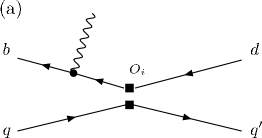
Figure 10: The other type of annihilation diagrams with operator insertion.

For ${(V-A)(V-A)}$ operators inserted in these diagrams, the results $M_{A2}^{(S,P)^{-}}$ are the same as $M_{A1}^{(S,P)^{-}}$,

$$M(B^{+}\to\rho^{+}\gamma)_{A2}^{j^{-}} = M_{A2_{4}}^{j(a)^{-}}(Q_{b})+M_{A2_{4}}^{j(b)^{-}}(Q_{d})+M_{A2_{4}}^{j(c)^{-}}(Q_{u})+M_{A2_{4}}^{j(d)^{-}}(Q_{u}),$$ (80)

$$M(B^{0}\to\rho^{0}\gamma)_{A2}^{j^{-}} = -\frac{1}{\sqrt{2}}\left[M_{A2_{4}}^{j(a)^{-}}(Q_{b})+M_{A2_{4}}^{j(b)^{-}}(Q_{d})+M_{A2_{4}}^{j(c)^{-}}(Q_{d})+M_{A2_{4}}^{j(d)^{-}}(Q_{d})\right],$$ (81)

$$M(B^{0}\to\omega\gamma)_{A2}^{j^{-}} = \frac{1}{\sqrt{2}}\left[M_{A2_{4}}^{j(a)^{-}}(Q_{b})+M_{A2_{4}}^{j(b)^{-}}(Q_{d})+M_{A2_{4}}^{j(c)^{-}}(Q_{d})+M_{A2_{4}}^{j(d)^{-}}(Q_{d})\right].$$ (82)

On the other hand, for ${(V-A)(V+A)}$ operators, the results are

$$M_{A2_{k}}^{S(a)^{+}}(Q_{b})=M_{A2_{k}}^{P(a)^{+}}(Q_{b})=0,$$ (83)

$$M_{A2_{k}}^{S(b)^{+}}(Q_{d}) = -M_{A2_{k}}^{S(b)^{+}}(Q_{d})$$ (84)

$$= F^{(0)}\xi_{p}\frac{3\sqrt{6}Q_{d}f_{B}\pi}{2M_{B}^{2}}\int dx_{2}\int db_{2}b_{2}\exp[-S_{V}(t_{A1}^{b})]S_{t}(x_{2})$$

$$\times a_{k}(t_{A1}^{b})\phi^{T}_{V}(x_{2})i\frac{\pi}{2}H^{(1)}_{0}(b_{2}B_{a}),$$

$$M_{A2_{k}}^{S(c)^{+}}(Q_{q})=M_{A2_{k}}^{P(c)^{+}}(Q_{q})=0,$$ (85)

$$M_{A2_{k}}^{S(d)^{+}}(Q_{q^{\prime}}) = -M_{A2_{k}}^{S(d)^{+}}(Q_{q^{\prime}})$$ (86)

$$= F^{(0)}\xi_{p}\frac{3\sqrt{6}Q_{q^{\prime}}f_{B}\pi}{2M_{B}^{2}}\int dx_{2}\int db_{2}b_{2}\exp[-S_{V}(t_{A1}^{d})]S_{t}(x_{2})$$

$$\times a_{k}(t_{A1}^{d})\phi^{T}_{V}(x_{2})i\frac{\pi}{2}H^{(1)}_{0}(b_{2}D_{a}),$$

then the amplitudes of this type with ${(V-A)(V+A)}$ vertex become as follows:

$$M(B^{+}\to\rho^{+}\gamma)_{A2}^{j^{+}} = M_{A2_{6}}^{j(a)^{+}}(Q_{b})+M_{A2_{6}}^{j(b)^{+}}(Q_{d})+M_{A2_{6}}^{j(c)^{+}}(Q_{u})+M_{A2_{6}}^{j(d)^{+}}(Q_{u}),$$ (87)

$$M(B^{0}\to\rho^{0}\gamma)_{A2}^{j^{+}} = -\frac{1}{\sqrt{2}}\left[M_{A2_{6}}^{j(a)^{+}}(Q_{b})+M_{A2_{6}}^{j(b)^{+}}(Q_{d})+M_{A2_{6}}^{j(c)^{+}}(Q_{d})+M_{A2_{6}}^{j(d)^{+}}(Q_{d})\right],$$ (88)

$$M(B^{0}\to\omega\gamma)_{A2}^{j^{+}} = \frac{1}{\sqrt{2}}\left[M_{A2_{6}}^{j(a)^{+}}(Q_{b})+M_{A2_{6}}^{j(b)^{+}}(Q_{d})+M_{A2_{6}}^{j(c)^{+}}(Q_{d})+M_{A2_{6}}^{j(d)^{+}}(Q_{d})\right].$$ (89)

In these type two cases, they are all color allowed decay modes.

4.5 The final decay amplitudes $M^{S}$ and $M^{P}$

Finally, we summarize the amplitudes $M^{j}$’s, $j=S,P$ for each decay mode:

$$M^{j}(B^{+}\to\rho^{+}\gamma) = M(B^{+}\to\rho^{+}\gamma)^{j}_{7\gamma}+M(B^{+}\to\rho^{+}\gamma)^{j}_{8g}+M(B^{+}\to\rho^{+}\gamma)^{j}_{1i}$$ (90)

$$+M(B^{+}\to\rho^{+}\gamma)^{j}_{2i}+M(B^{+}\to\rho^{+}\gamma)^{j}_{A}+M(B^{+}\to\rho^{+}\gamma)^{j-}_{A2}$$

$$+M(B^{+}\to\rho^{+}\gamma)^{j+}_{A2}~{},$$

$$M^{j}(B^{0}\to\rho^{0}\gamma) = M(B^{0}\to\rho^{0}\gamma)^{j}_{7\gamma}+M(B^{0}\to\rho^{0}\gamma)^{j}_{8g}+M(B^{0}\to\rho^{0}\gamma)^{j}_{1i}$$ (91)

$$+M(B^{0}\to\rho^{0}\gamma)^{j}_{2i}+M(B^{0}\to\rho^{0}\gamma)^{j}_{A}+M(B^{0}\to\rho^{0}\gamma)^{j-}_{A1}$$

$$+M(B^{0}\to\rho^{0}\gamma)^{j+}_{A1}+M(B^{0}\to\rho^{0}\gamma)^{j-}_{A2}+M(B^{0}\to\rho^{0}\gamma)^{j+}_{A2}~{},$$

$$M^{j}(B^{0}\to\omega\gamma) = M(B^{0}\to\omega\gamma)^{j}_{7\gamma}+M(B^{0}\to\omega\gamma)^{j}_{8g}+M(B^{0}\to\omega\gamma)^{j}_{1i}$$ (92)

$$+M(B^{0}\to\omega\gamma)^{j}_{2i}+M(B^{0}\to\omega\gamma)^{j}_{A}+M(B^{0}\to\omega\gamma)^{j-}_{A1}$$

$$+M(B^{0}\to\omega\gamma)^{j+}_{A1}+M(B^{0}\to\omega\gamma)^{j-}_{A2}+M(B^{0}\to\omega\gamma)^{j+}_{A2}~{}.$$

5 Numerical analysis and discussions

In our numerical calculations, the choice of the input parameters is summarized in Tab.1, where $\lambda$, $A$, $\rho$ and $\eta$ are CKM parameters in Wolfenstein parametrization [19], and $\bar{\rho}=\rho(1-\frac{1}{2}\lambda^{2})$, $\bar{\eta}=\eta(1-\frac{1}{2}\lambda^{2})$. Their values can be found in PDG [20]. The numerical results for each decay amplitudes ${M_{i}^{j}}$ in the ${B^{0}\to\rho^{0}\gamma}$ (Tab.2), ${B^{0}\to\omega\gamma}$ (Tab.3), and ${B^{+}\to\rho^{+}\gamma}$ (Tab.4) in unit of ${10^{-6}\mbox{GeV}^{-2}}$ are as follows.

When we estimate the physical quantities like branching ratio, direct CP asymmetry, and isospin breaking effect, we take into account the following theoretical errors. The detailed discussions for the errors are in [21]. First, we change the input parameters; the decay constants and ${\omega_{B}}$ in the $B$ meson wave function, and we regard the 15% error in each cases at the amplitude level. This generates the theoretical error for the physical quantities about 40% in the branching ratio, 5% in the direct CP asymmetry, and 30% in the isospin breaking.

Second, we estimate that the higher order effects in perturbation expansion to be about 15% error in the amplitude. This leads to about 30% in the branching ratio and in the isospin breaking. Here, the cancellation of the higher order effects can occur by taking the ratio of the decay width in the direct CP asymmetry. Then we can neglect these uncertainties for the CP asymmetry.

CKM parameters and QCD constant
$\begin{array}[]{ccccc}\lambda&A&\bar{\rho}&\bar{\eta}&\Lambda_{\overline{\mathrm{MS}}}^{(f=4)}\\ 0.2196&0.819&0.20\pm 0.09&0.33\pm 0.05&250~{}\mbox{MeV}\end{array}$
Meson decay constants
$\begin{array}[]{ccccc}f_{B}&f_{\rho}&f_{\rho}^{T}&f_{\omega}&f_{\omega}^{T}\\ 190~{}\mbox{MeV}&220~{}\mbox{MeV}&160~{}\mbox{MeV}&195~{}\mbox{MeV}&160~{}\mbox{MeV}\end{array}$
Masses
$\begin{array}[]{ccccc}M_{W}&M_{B}&M_{\rho}&M_{\omega}&m_{c}\\ 80.41~{}\mbox{GeV}&5.28~{}\mbox{GeV}&0.77~{}\mbox{GeV}&0.78~{}\mbox{GeV}&1.2~{}\mbox{MeV}\end{array}$
$B$ meson life time
$\begin{array}[]{cc}\tau_{B^{0}}&\tau_{B^{\pm}}\\ 1.542~{}\mbox{ps}&1.674~{}\mbox{ps}\end{array}$

Table 1: Summary of input parameters

Third, the error due to the CKM parameter uncertainties ${\bar{\rho}}$ and ${\bar{\eta}}$ generates about 30% error in the branching ratios and direct CP asymmetry, and $100$% error in the isospin breaking effects. We can see that the uncertainty which comes from the CKM parameters are large compared to ${B\to K^{*}\gamma}$ decay modes [21]. The reason for it is that the all CKM matrix elements which concern ${B\to\rho(\omega)\gamma}$ decay (${V_{tb}^{*}V_{td}}$, ${V_{cb}^{*}V_{cd}}$, ${V_{ub}^{*}V_{ud}}$) are comparable, and the three angles of the KM unitarity triangle are sizable: the situation is different from in ${B\to K^{*}\gamma}$ decay. The conditions mentioned above make the uncertainty from the CKM parameters large.

In the end, we also take into account the uncertainties from ${u}$ quark loop contributions like Figs.6 and 7. We guess that the nonperturbative effects in the ${u}$ quark loop might lead to large hadronic uncertainties. So, we introduce the 100% theoretical error at the amplitude level. This theoretical uncertainty leads to small uncertainties (about 2%) for the branching ratio, ${80}$% errors for the CP asymmetry, and about 3% errors for the isospin breaking effects.

	${M_{i}^{S}/F^{(0)}\xi_{q}}$			${M_{i}^{P}/F^{(0)}\xi_{q}}$
${M_{7\gamma}^{S}/F^{(0)}\xi_{t}}$	${M_{8g}^{S}/F^{(0)}\xi_{t}}$	${\sum_{i=1,2}M_{Ai}^{S}/F^{(0)}\xi_{t}}$	${M_{7\gamma}^{P}/F^{(0)}\xi_{t}}$	${M_{8g}^{P}/F^{(0)}\xi_{t}}$	${\sum_{i=1,2}M_{Ai}^{P}/F^{(0)}\xi_{t}}$
-172.12	-0.44-1.19i	-7.76 - 3.45 i	172.12	0.48+1.18i	7.55+ 3.47 i
${M_{1c}^{S}/F^{(0)}\xi_{c}}$	${M_{2c}^{S}/F^{(0)}\xi_{c}}$		${M_{1c}^{P}/F^{(0)}\xi_{c}}$	${M_{2c}^{P}/F^{(0)}\xi_{c}}$
0.39+1.01i	-1.21+8.84i		-0.08-0.97i	0.42-6.28i
${M_{1u}^{S}/F^{(0)}\xi_{u}}$	${M_{2u}^{S}/F^{(0)}\xi_{u}}$	${M_{A}^{S}/F^{(0)}\xi_{u}}$	${M_{1u}^{P}/F^{(0)}\xi_{u}}$	${M_{2u}^{P}/F^{(0)}\xi_{u}}$	${M_{A}^{P}/F^{(0)}\xi_{u}}$
1.35+2.06i	-1.11-27.76i	1.14-0.01i	-1.13-1.98i	-0.73+28.15i	-2.47+0.17i

Table 2: The numerical results for ${B^{0}\to\rho^{0}\gamma}$ decay at ${\bar{\rho}=0.20}$, ${\bar{\eta}=0.33}$, ${\omega_{B}=0.40}$GeV.

	${M_{i}^{S}/F^{(0)}\xi_{q}}$			${M_{i}^{P}/F^{(0)}\xi_{q}}$
${M_{7\gamma}^{S}/F^{(0)}\xi_{t}}$	${M_{8g}^{S}/F^{(0)}\xi_{t}}$	${\sum_{i=1,2}M_{Ai}^{S}/F^{(0)}\xi_{t}}$	${M_{7\gamma}^{P}/F^{(0)}\xi_{t}}$	${M_{8g}^{P}/F^{(0)}\xi_{t}}$	${\sum_{i=1,2}M_{Ai}^{P}/F^{(0)}\xi_{t}}$
161.59	0.44+1.21i	7.73 + 3.45 i	-161.59	-0.47-1.18i	-7.71 - 3.42 i
${M_{1c}^{S}/F^{(0)}\xi_{c}}$	${M_{2c}^{S}/F^{(0)}\xi_{c}}$		${M_{1c}^{P}/F^{(0)}\xi_{c}}$	${M_{2c}^{P}/F^{(0)}\xi_{c}}$
-0.46-0.99i	1.21-8.58i		0.12+0.99i	-0.36+6.35i
${M_{1u}^{S}/F^{(0)}\xi_{u}}$	${M_{2u}^{S}/F^{(0)}\xi_{u}}$	${M_{A}^{S}/F^{(0)}\xi_{u}}$	${M_{1u}^{P}/F^{(0)}\xi_{u}}$	${M_{2u}^{P}/F^{(0)}\xi_{u}}$	${M_{A}^{P}/F^{(0)}\xi_{u}}$
-1.03-2.10i	1.64+ 27.00i	1.04-0.01i	1.06+2.10i	0.05-27.45i	-2.25+0.12i

Table 3: The numerical results for ${B^{0}\to\omega\gamma}$ decay at ${\bar{\rho}=0.20}$, ${\bar{\eta}=0.33}$, ${\omega_{B}=0.40}$GeV.

	${M_{i}^{S}/F^{(0)}\xi_{q}}$			${M_{i}^{P}/F^{(0)}\xi_{q}}$
${M_{7\gamma}^{S}/F^{(0)}\xi_{t}}$	${M_{8g}^{S}/F^{(0)}\xi_{t}}$	${\sum_{i=1,2}M_{Ai}^{S}/F^{(0)}\xi_{t}}$	${M_{7\gamma}^{P}/F^{(0)}\xi_{t}}$	${M_{8g}^{P}/F^{(0)}\xi_{t}}$	${\sum_{i=1,2}M_{Ai}^{P}/F^{(0)}\xi_{t}}$
243.72	4.76-3.12i	-4.61 - 2.73 i	-243.72	-4.56+3.15i	4.08 + 2.42 i
${M_{1c}^{S}/F^{(0)}\xi_{c}}$	${M_{2c}^{S}/F^{(0)}\xi_{c}}$		${M_{1c}^{P}/F^{(0)}\xi_{c}}$	${M_{2c}^{P}/F^{(0)}\xi_{c}}$
-0.74+2.70i	1.70-15.36i		1.51-3.02i	-0.48+ 11.23i
${M_{1u}^{S}/F^{(0)}\xi_{u}}$	${M_{2u}^{S}/F^{(0)}\xi_{u}}$	${M_{A}^{S}/F^{(0)}\xi_{u}}$	${M_{1u}^{P}/F^{(0)}\xi_{u}}$	${M_{2u}^{P}/F^{(0)}\xi_{u}}$	${M_{A}^{P}/F^{(0)}\xi_{u}}$
-2.39+ 6.05i	1.70+39.28i	37.28-7.90i	2.65-5.19i	0.99-39.80i	-55.47-0.37i

Table 4: The numerical results for ${B^{+}\to\rho^{+}\gamma}$ decay at ${\bar{\rho}=0.20}$, ${\bar{\eta}=0.33}$, ${\omega_{B}=0.40}$GeV.

Then the total theoretical error for each physical quantity becomes as about 60% in the branching ratio, 85% in the CP asymmetry, and 100% in the isospin breaking effects.

With the amplitudes $M^{S}$ and $M^{P}$ defined in Eq.(5), the total decay rate of $B\to\rho(\omega)\gamma$ is given by

$$\Gamma=\frac{|M^{S}|^{2}+|M^{P}|^{2}}{8\pi M_{B}}\;,$$ (93)

and the relevant decay branching ratio is defined to be

$$Br=\frac{\tau_{B}}{\hbar}\Gamma\;,$$ (94)

where $\tau_{B}$ is the mean lifetime of the $B$ meson. The branching ratios for neutral and charged modes are defined as

$$Br(B^{\pm}\to\rho^{\pm}\gamma) = \frac{1}{2}\left[Br(B^{+}\to\rho^{+}\gamma)+Br(B^{-}\to\rho^{-}\gamma)\right],\hskip 19.91692pt$$ (95)

$$Br(B^{0}\to\rho^{0}\gamma) = \frac{1}{2}\left[Br(B^{0}\to\rho^{0}\gamma)+Br(\bar{B}^{0}\to\rho^{0}\gamma)\right],\hskip 19.91692pt$$ (96)

and its’ predicted values become as

$$Br(B^{0}\to\rho^{0}\gamma)=(1.2\pm 0.7)\times 10^{-6},$$ (97)

$$Br(B^{0}\to\omega\gamma)=(1.1\pm 0.6)\times 10^{-6},$$ (98)

$$Br(B^{\pm}\to\rho^{\pm}\gamma)=(2.5\pm 1.5)\times 10^{-6}.$$ (99)

The direct CP asymmetry is defined by

$$A_{cp}(B^{\pm}\to\rho^{\pm}\gamma)=\frac{\Gamma(B^{-}\to\rho^{-}\gamma)-\Gamma(B^{+}\to\rho^{+}\gamma)}{\Gamma(B^{-}\to\rho^{-}\gamma)+\Gamma(B^{+}\to\rho^{+}\gamma)}$$ (100)

for charged $B$ meson decays, and

$$A_{cp}(B^{0}\to\rho^{0}(\omega)\gamma)=\frac{\Gamma(\bar{B}^{0}\to\rho^{0}(\omega)\gamma)-\Gamma(B^{0}\to\rho^{0}(\omega)\gamma)}{\Gamma(\bar{B}^{0}\to\rho^{0}(\omega)\gamma)+\Gamma(B^{0}\to\rho^{0}(\omega)\gamma)}$$

for neutral $B$ meson decays. The numerical results for these CP asymmetries in $B\to\rho\gamma$ and $\omega\gamma$ are as follows:

$$A_{cp}(B^{0}\to\rho^{0}\gamma) = (17.6\pm 15.0)\%$$ (102)

$$A_{cp}(B^{0}\to\omega\gamma) = (17.9\pm 15.2)\%$$ (103)

$$A_{cp}(B^{\pm}\to\rho^{\pm}\gamma) = (17.7\pm 15.0)\%.$$ (104)

Next we discuss the isospin breaking effect in $B\to\rho\gamma$ decay. The isospin relation requires that the branching ratio of $B^{+}\to\rho^{+}\gamma$ is two times of $B^{0}\to\rho^{0}\gamma$. However, the contribution of the annihilation diagrams can violate this isospin relation. We can define the isospin breaking parameter as

$$\Delta_{0+}(B\to\rho\gamma) = \frac{\Gamma(B^{+}\to\rho^{+}\gamma)}{2\Gamma(B^{0}\to\rho^{0}\gamma)}-1,$$ (105)

$$\Delta_{0-}(B\to\rho\gamma) = \frac{\Gamma(B^{-}\to\rho^{-}\gamma)}{2\Gamma(\bar{B}^{0}\to\rho^{0}\gamma)}-1,$$ (106)

$$\Delta(\rho\gamma) = \frac{\Delta_{0+}+\Delta_{0-}}{2}.$$ (107)

If isospin relation is maintained, $\Delta(\rho\gamma)$ defined above should be zero. Our numerical result for isospin effects is

$$\Delta(\rho\gamma)=-(5.4\pm 5.4)\%.$$ (108)

6 Conclusion

In this paper, we calculated the branching ratio, direct CP asymmetry and isospin breaking effects within the standard model using the pQCD approach. Our predictions for the physical quantities are summarized in Tab.5.

Numerical results

Branching ratio

$\begin{array}[]{ccccc}B^{0}\to\rho^{0}\gamma&&B^{0}\to\omega\gamma&&B^{+}\to\rho^{+}\gamma\\ (1.2\pm 0.7)\times 10^{-6}&&(1.1\pm 0.6)\times 10^{-6}&&(2.5\pm 1.5)\times 10^{-6}\end{array}$

Direct CP asymmetry

$\begin{array}[]{ccccc}B^{0}\to\rho^{0}\gamma&&B^{0}\to\omega\gamma&&B^{+}\to\rho^{+}\gamma\\ (17.6\pm 15.0)\%{}{}{}{}&&(17.9\pm 15.2)\%{}{}{}{}&&(17.7\pm 15.0)\%{}{}{}{}\end{array}$

Isospin breaking effects

$\begin{array}[]{c}\Delta(\rho\gamma)=-(5.4\pm 5.4)\%\end{array}$

Table 5: The conclusion related to the branching ratio, CP asymmetry, and isospin breaking effects.

The ${B\to\rho}$ magnetic form factor ${T_{1}^{\rho}}$ is defined as

$$\langle\rho(P_{2},\epsilon_{K^{*}})\mid iq^{\nu}\bar{d}\sigma_{\mu\nu}b\mid B(P_{1})\rangle=-iT_{1}^{\rho}(0)\epsilon_{\mu\alpha\beta\rho}\epsilon_{\rho}^{\alpha}P^{\beta}q^{\rho}$$ (109)

where ${P=P_{1}+P_{2}}$, ${q=P_{1}-P_{2}}$, and the value computed by the pQCD approach is ${T_{1}^{\rho}=}$ ${0.26\pm 0.07}$. The value from the light-cone-QCD sum rule (LCSR) is ${T_{1}^{\rho}=0.29\pm 0.04}$ [22], then our value of the form factor is in good agreement with LCSR. The branching ratios only from ${O_{7\gamma}}$ become ${Br(B^{\pm}\to\rho^{\pm}\gamma)=(2.4\pm 1.2)\times 10^{-6}}$, ${Br(B^{0}\to\rho^{0}\gamma)=(1.1\pm 0.5)\times 10^{-6}}$, and
${Br(B^{0}\to\omega\gamma)=(1.0\pm 0.5)\times 10^{-6}}$; then by comparing them to Eqs.(97)-(99), we can see that ${O_{7\gamma}}$ contributions are dominant.

The subtle excess of the branching ratio of ${B^{0}\to\rho^{0}\gamma}$ compared to that of ${B^{0}\to\omega\gamma}$ is caused by the following two reasons: (1) the difference in the meson mass and decay constants between ${\rho}$ and ${\omega}$; (2) the annihilation contributions from ${O_{1}}$ to ${O_{6}}$. We examined these possibilities, and concluded that the subtle excess of the branching ratio mainly comes from (1), and the effects from (2) are very small.

The isospin breaking effect ${\Delta(\rho\gamma)}$ is caused by the contributions ${O_{8g}}$ (Fig.5), charm and up quark loop contributions (Fig.6), and ${O_{1}\sim O_{6}}$ annihilation contributions (Figs.8-10). Our prediction for this quantity is given in Eq.(108). The main contributions to the isospin breaking effect come from ${O_{1}\sim O_{6}}$ annihilation diagrams. In general, we can expect that the annihilation contributions are suppressed by the factor ${O(m_{q}/m_{b})}$, where ${m_{q}=m_{u},~{}m_{d}}$. In our computation, weak annihilations caused by ${O_{3}\sim O_{6}}$ are about 5% and tree annihilations caused by ${O_{1},O_{2}}$ are 1% in the neutral modes, (see Tabs.2 and 3); on the other hand, in the charged mode, weak annihilations are about 2% and tree annihilations are about 20%; this contribution is large because it is a color allowed process (see Tab.4) in the amplitudes. If we neglect ${O_{1}\sim O_{6}}$ annihilation contributions, the isospin breaking effects have the opposite sign: ${\Delta(\rho\gamma)=+(3.4\pm 3.4)\%}$. Thus the annihilation contributions are crucial to the isospin breaking effects.

When we compare our results with the world averages of experimental data for the ${b\to d\gamma}$ decay modes [9], our results for the branching ratios are somewhat large. For now, we shall not worry about it for the following reason: Note that our conclusion given in Tab.5,

$$Br(B^{0}\to\rho^{0}\gamma)\approx Br(B^{0}\to\omega\gamma)\approx\frac{1}{2}Br(B^{+}\to\rho^{+}\gamma),$$ (110)

follows from the isospin symmetry and the fact that contribution from the ${O_{7\gamma}}$ operator dominates over all other contributions. A similar conclusion has been derived from the ${B\to K^{*}\gamma}$ decay mode [23], and experimental results for ${B\to K^{*}\gamma}$ agree with our conclusions. While the error is large, the relationships indicated by Eq.(110) are not obviously seen in the recent experimental data. We thus feel it is too early to discuss the validity of Eq.(110). We expect that the data may change by about a factor two if Eq.(110) is approximately valid.

Appendix A Wave function

In the calculation of the decay amplitude, the wave functions of meson states can be defined via nonlocal matrix elements of quark operators sandwiched between meson states and vacuum. Next let us introduce the wave functions needed in this work.

The two leading-twist B meson wave functions can be defined through the following nonlocal matrix element [24]:

$$\int_{0}^{1}\frac{d^{4}z}{(2\pi)^{4}}e^{i\bf{k_{1}}\cdot z}\langle 0|\bar{q}_{\alpha}(z)b_{\beta}(0)|\bar{B}(p_{B})\rangle$$

$$\hskip 14.22636pt=\frac{i}{\sqrt{2N_{c}}}\left\{(\not p_{B}+M_{B})\gamma_{5}\left[\frac{\not v}{\sqrt{2}}\phi_{B}^{+}({\bf k_{1}})+\frac{\not n}{\sqrt{2}}{\phi}_{B}^{-}({\bf k_{1}})\right]\right\}_{\beta\alpha}$$

$$\hskip 14.22636pt=-\frac{i}{\sqrt{2N_{c}}}\left\{(\not p_{B}+M_{B})\gamma_{5}\left[\phi_{B}({\bf k_{1}})+\sqrt{2}{\not n}\bar{\phi}_{B}({\bf k_{1}})\right]\right\}_{\beta\alpha},$$

(111)

where $\bf{k_{1}}$ is the momentum of the light quark in the $B$ meson, and $n=(1,0,{\bf 0_{T}})$, and $v=(0,1,{\bf 0_{T}})$. The normalization conditions for these two wave functions are

$$\int d^{4}k_{1}\phi_{B}^{+}({\bf k_{1}})=\frac{f_{B}}{2\sqrt{2N_{c}}},~{}~{}~{}\int d^{4}k_{1}\phi_{B}^{-}({\bf k_{1}})=\frac{f_{B}}{2\sqrt{2N_{c}}}.$$ (112)

The relations between $\phi_{B}$, $\bar{\phi}_{B}$ and $\phi_{B}^{+}$, $\phi_{B}^{-}$ are

$$\phi_{B}=\phi_{B}^{+}~{},~{}~{}\bar{\phi}_{B}=\frac{\phi_{B}^{+}-\phi_{B}^{-}}{2}.$$ (113)

In practice it is convenient to work in the impact parameter $b$ space rather than the transverse momentum space ($k_{\bot}$-space). So we make a Fourier transformation $\int d^{2}k_{\bot}e^{-i{\bf k}_{\bot}\cdot{\bf b}}$ to transform the wave functions and hard amplitude into $b$-space. Then the normalization condition for $\phi_{B}$ and $\bar{\phi}_{B}$ can be expressed as

$$\int_{0}^{1}dx\phi_{B}(x,b=0)=\frac{f_{B}}{2\sqrt{2N_{c}}},~{}~{}~{}\int_{0}^{1}dx\bar{\phi}_{B}(x,b=0)=0\;.$$ (114)

$\phi_{B}$ and $\bar{\phi}_{B}$ include bound state effects; they are controlled by nonperturbative dynamics. They can be treated by models or by solving the equation of motion in heavy quark limit.

In some particular models, $\phi_{B}$ and $\bar{\phi}_{B}$ can be selected such that the contribution of $\bar{\phi}_{B}$ is the next-to-leading-power $\bar{\Lambda}/m_{B}$ [25]. In this case the contribution of $\bar{\phi}_{B}$ can be neglected at leading-power. Hence, only $\phi_{B}$ is considered in this case. We adopt the model for $\phi_{B}$ in the impact parameter $b$ space, which is widely used in the study of $B$ decays in the perturbative QCD approach [14]

$$\phi_{B}(x,b)=N_{B}x^{2}(1-x)^{2}\mathrm{exp}\left[-\frac{1}{2}\left(\frac{xM_{B}}{\omega_{B}}\right)^{2}-\frac{\omega_{B}^{2}b^{2}}{2}\right]\;,$$ (115)

where the shape parameter $\omega_{B}$ has been determined as $\omega_{B}=0.40\mathrm{GeV}$, and $N_{B}$ is the normalization constant.

In $B\to\rho\gamma$ and $\omega\gamma$ decays, $\rho$ and $\omega$ meson can only be transversely polarized. We only need to consider the wave function of transversely polarized $\rho$ or $\omega$ meson. They are defined by

$$\langle\rho/\omega(P,\epsilon_{V}^{T})|\bar{d_{\alpha}}(z)u_{\beta}(0)|0\rangle=\frac{1}{\sqrt{2N_{c}}}\int_{0}^{1}dxe^{ixP\cdot z}\Big{[}M_{V}[\ooalign{\hfil/\hfil\crcr$\epsilon$}_{V}^{\ast T}]\phi_{V}^{v}(x)$$ (118)

$$\hskip 128.0374pt+[\ooalign{\hfil/\hfil\crcr$\epsilon$}_{V}^{\ast T}\hskip 2.84526pt\ooalign{\hfil/\hfil\crcr$P$}]\phi_{V}^{T}(x)-\frac{M_{V}}{P\cdot n_{+}}i\epsilon_{\mu\nu\rho\sigma}[\gamma^{5}\gamma^{\mu}]\epsilon_{V}^{T\nu}P^{\rho}n_{+}^{\sigma}\phi_{V}^{a}(x)\Big{]}.\hskip 28.45274pt$$ (123)

For the transverse $\rho$ meson, the distribution amplitudes are given as [15]:

$$\phi_{\rho}^{T}(x) = \frac{3f_{\rho}^{T}}{\sqrt{6}}x(1-x)\left[1+0.2C_{2}^{3/2}(t)\right],$$ (124)

$$\phi_{\rho}^{v}(x) = \frac{f_{\rho}}{2\sqrt{6}}\Big{[}\frac{3}{4}(1+t^{2})+0.24(3t^{2}-1)$$ (125)

$$\hskip 42.67912pt+0.12(3-30t^{2}+35t^{4})\Big{]},$$

$$\phi_{\rho}^{a}(x) = \frac{3f_{\rho}}{4\sqrt{6}}~{}t\left[1+0.93(10x^{2}-10x+1)\right],$$ (126)

where $t=1-2x$ and

$$\phi_{V}^{T}(x)=\frac{f_{V}^{T}}{2\sqrt{2N_{c}}}\phi_{\perp},\hskip 22.76219pt\phi_{V}^{v}(x)=\frac{f_{V}}{2\sqrt{2N_{c}}}g_{\perp}^{(v)},\hskip 22.76219pt\phi_{V}^{a}(x)=\frac{f_{V}}{8\sqrt{2N_{c}}}\frac{d}{dx}g_{\perp}^{(a)}.$$

We use ${\epsilon_{0123}=1}$ and set the normalization condition about ${\phi_{i}=\{\phi_{\perp},g_{\perp}^{(v)},g_{\perp}^{(a)}\}}$ as

$$\int_{0}^{1}dx\phi_{i}(x)=1.$$ (127)

The Gegenbauer polynomial is defined by

$$C_{2}^{3/2}(t)=\frac{3}{2}(5t^{2}-1).$$ (128)

Appendix B Some Functions

The expressions for some functions are presented in this appendix. In our numerical calculation, we use the leading order ${\alpha_{s}}$ formula as

$$\alpha_{s}(\mu)=\frac{2\pi}{\beta_{0}\ln(\mu/\Lambda_{n_{f}})},\hskip 14.22636pt\beta_{0} = \frac{33-2n_{f}}{3},$$ (129)

and we fix the number of the flavor as ${n_{f}=4}$. The explicit expression for Sudakov factor ${s(t,b)}$ is given by [26] as follows:

$$s(t,b) = \int^{t}_{1/b}\frac{d\mu}{\mu}\left[\ln{\left(\frac{t}{\mu}\right)}A(\alpha_{s}(\mu))+B(\alpha_{s}(\mu))\right],$$ (130)

$$A = C_{F}\frac{\alpha_{s}}{\pi}+\left(\frac{\alpha_{s}}{\pi}\right)^{2}\left[\frac{67}{9}-\frac{{\pi}^{2}}{3}-\frac{10}{27}n_{f}+\frac{2}{3}\beta_{0}\ln\left(\frac{e^{\gamma}_{E}}{2}\right)\right],$$ (131)

$$B = \frac{2}{3}\frac{\alpha_{s}}{\pi}\ln\left(\frac{e^{2\gamma_{E}}-1}{2}\right),$$ (132)

where ${\gamma_{E}=0.5722}$ is Euler constant and ${C_{F}=4/3}$ is color factor. The meson wave function including summation factor has energy dependence,

$$\phi_{B}(x_{1},b_{1},t) = \phi_{B}(x_{1},b_{1})\exp{[-S_{B}(t)]},$$ (133)

$$\phi_{V}(x_{2},t) = \phi_{V}(x_{2})\exp{[-S_{V}(t)]},$$ (134)

and the total functions including Sudakov factor and ultraviolet divergences are

$$S_{B}(t) = s(x_{1}P_{1}^{-},b_{1})+2\int^{t}_{1/b_{1}}\frac{d\bar{\mu}}{\bar{\mu}}\gamma(\alpha_{s}(\bar{\mu})),$$ (135)

$$S_{V}(t) = s(x_{2}P_{2}^{-},b_{2})+s((1-x_{2})P_{2}^{-},b_{2})+2\int^{t}_{1/b_{2}}\frac{d\bar{\mu}}{\bar{\mu}}\gamma(\alpha_{s}(\bar{\mu})).$$ (136)

Threshold factor is expressed as below [23, 27], and we take the value ${c=0.4}$:

$$S_{t}(x)=\frac{2^{1+2c}\Gamma(3/2+c)}{\sqrt{\pi}\Gamma(1+c)}[x(1-x)]^{c}.$$ (137)

References

- [1] A. B. Carter and A. I. Sanda, Phys. Rev. D 23, 1567 (1981).
- [2] I. I. Y. Bigi and A. I. Sanda, Nucl. Phys. B 193, 85 (1981).
- [3] K. Abe et al. [Belle Collaboration], arXiv:hep-ex/0308036.
- [4] G. Raven, eConf C0304052, WG417 (2003) [arXiv:hep-ex/0307067].
- [5] B. Aubert et al. [BABAR Collaboration], arXiv:hep-ex/0412037.
- [6] A. Bevan [BaBar Collaboration], arXiv:hep-ex/0411090.
- [7] K. Abe et al. [Belle Collaboration], arXiv:hep-ex/0411049.
- [8] R. Ammar et al. [CLEO Collaboration], Phys. Rev. Lett. 71, 674 (1993). M. S. Alam et al. [CLEO Collaboration], Phys. Rev. Lett. 74, 2885 (1995).
- [9] Heavy Flavor Averaging Group (HFAG), the data of the summer in 2005.
- [10] C. Greub, H. Simma, D. Wyler, Nucl. Phys. B434, 39 (1995); J. Milana, Phys. Rev .D53, 1403 (1996); A. Ali, V.M. Braun, Phys. Lett. B359, 223 (1995); J.F. Donoghue, E. Golowich, A.A. Petrov, Phys. Rev. D55, 2657 (1997); T. Huang, Z.H. Li, H.D. Zhang, J. Phys. G25, 1179 (1999); B. Grinstein and D. Pirjol, D 62, 093002 (2000) [arXiv:hep-ph/0002216]; D. Pirjol, Phys. Lett. B 487, 306 (2000) [arXiv:hep-ph/0006315]; A. Ali, A.Y. Parkhomenko, Eur. Phys. J. C23, 89 (2002); S.W. Bosch, G. Buchalla, Nucl. Phys. B621, 459 (2002); M. Beyer, D. Melikhov, N. Nikitin, B. Stech, Phys. Rev. D64, 094006 (2001); S.W. Bosch, eprint hep-ph/031031; A.Ali, E. Lunghi, A.Y. Parkhomenko, eprint hep-ph/0405075; M. Beneke, T. Feldmann and D. Seidel, arXiv:hep-ph/0412400.
- [11] A. Ali, L.T. Handoko, D. London, Phys. Rev. D63, 014014 (2000); L.T. Handoko, Nucl. Phys. Proc. Suppl. 93, 296 (2001); A. Arhrib, C.K. Chua, W.S. Hou, Eur. Phys. J. C21, 567 (2001); A. Ali, E. Lunghi, Eur. Phys. J. C26, 195 (2002); Z. Xiao, C. Zhuang, Eur. Phys. J. C33349 (2004); C.S. Kim, Y.G. Kim, K.Y. Lee, eprint hep-ph/0407060.
- [12] H.N. Li and H.L. Yu, Phys. Rev. Lett. 74 (1995) 4388; H.N. Li and H.L. Yu, Phys. Lett. B353 (1995) 301; H.N. Li, Phys. Rev. D52 (1995) 3958; H.N. Li and H.L. Yu, Phys. Rev. D53 (1996) 2480.
- [13] C.H. Chang and H.N. Li, Phys. Rev. D55 (1997) 5577; T.W. Yeh and H.N. Li, Phys. Rev. D56 (1997) 1615; M. Nagashima, H.N. Li, Phys. Rev. D67, 034001 (2003).
- [14] Y.Y. Keum, H.N. Li, A.I. Sanda, Phys. Lett. B504, 6 (2001); Phys. Rev. D63, 054008 (2001); Phys. Rev. D63, 074006 (2001); C.D. Lü, K. Ukai, M.Z. Yang, Phys. Rev. D63, 074009 (2001).
- [15] P. Ball, V.M. Braun, Y. Koike, and K. Tanaka, Nucl. Phys. B529 (1998) 323.
- [16] For a review, see G. Buchalla, A.J. Buras, and M.E. Lautenbacher, Rev. Mod. Phys. 68, 1125 (1996).
- [17] J. Liu and Y.P. Yao, Phys. Rev. D42, 1485 (1990); H. Simma and D. Wyler, Nucl. Phys. B344, 283 (1990).
- [18] H.n. Li and G.L. Lin, Phys. Rev. D60, 054001 (1999). Rev. D66, 0094010 (2002).
- [19] L. Wolfenstein, Phys. Rev. Lett. 51, 1945 (1983).
- [20] S. Eidelman et al. [Particle Data Group], Phys. Lett. B 592 (2004) 1.
- [21] Y. Y. Keum, M. Matsumori and A. I. Sanda, Phys. Rev. D 72 (2005) 014013 [arXiv:hep-ph/0406055].
- [22] P. Ball and V. M. Braun, Phys. Rev. D 58, 094016 (1998) [arXiv:hep-ph/9805422].
- [23] Y. Y. Keum, H. N. Li and A. I. Sanda, Phys. Rev. D 63 (2001) 054008 [arXiv:hep-ph/0004173].
- [24] A.G. Grozin, M. Neubert, Phys. Rev. D55, 272 (1997); M. Beneke, T. Feldmann, Nucl. Phys. B592, 3 (2001).
- [25] T. Kurimoto, Hsiang-nan Li, A.I. Sanda, Phys. Rev. D67, 054028 (2003).
- [26] J. Botts and G. Sterman, Nucl. Phys. B 325, 62 (1989).
- [27] H. n. Li, Phys. Rev. D 66, 094010 (2002) [arXiv:hep-ph/0102013].