Two-boson truncation of Pauli–Villars-regulated Yukawa theory

Abstract

We apply light-front quantization, Pauli–Villars regularization, and numerical techniques to the nonperturbative solution of the dressed-fermion problem in Yukawa theory in $3+1$ dimensions. The solution is developed as a Fock-state expansion truncated to include at most one fermion and two bosons. The basis includes a negative-metric heavy boson and a negative-metric heavy fermion in order to provide the necessary cancellations of ultraviolet divergences. The integral equations for the Fock-state wave functions are solved by reducing them to effective one-boson–one-fermion equations for eigenstates with $J_{z}=1/2$. The equations are converted to a matrix equation with a specially tuned quadrature scheme, and the lowest mass state is obtained by diagonalization. Various properties of the dressed-fermion state are then computed from the nonperturbative light-front wave functions. This work is a major step in our development of Pauli–Villars regularization for the nonperturbative solution of four-dimensional field theories and represents a significant advance in the numerical accuracy of such solutions.

and

1 Introduction

One of the important unsolved problems in obtaining bound-state solutions in quantum field theories such as quantum chromodynamcs is how to implement ultraviolet renormalization nonperturbatively. The central difficulty is that any truncation or approximation of the theory which breaks Lorentz symmetries, such as the truncation of the Fock space, introduces spurious divergences. Quadratic divergences can occur in the approximated theory, even when the renormalizable perturbative Feynman theory has only logarithmic divergences. Such problems arise even when one uses light-front quantization methods which retain the maximal set of kinematical Lorentz symmetries. A systematic light-front approach to renormalization, developed by Glazek, Harindranath, Perry, and Wilson [1, 2, 3], is to introduce new effective interactions which act as counterterms to control the ultraviolet behavior of the approximated theory. However, this method is challenging to implement in practice, because the large set of new effective interactions, some of which have a nonlocal structure, can require so much input data that the ability to make predictions is seriously compromised.

Another important nonperturbative approach is to cast the bound-state problem in the form of an effective Bethe–Salpeter equation and use Schwinger–Dyson methods to construct the effective renormalized quark and gluon propagators of the theory, including running quark masses consistent with chiral symmetry breaking [4, 5]. In principle, this method could be used to predict the light-front wave functions needed for QCD phenomenology, if one evaluates the Minkowski-space Bethe–Salpeter wave functions at fixed light-front time. However, it has been difficult to carry out this program in practice since the analyses have only been done in ladder gluon-exchange approximation and in Euclidean space. The full structure of nonperturbative renormalization will require consideration of higher-order kernels.

Lattice gauge theory [6] is currently the most successful method for solving gauge theories; it has a systematic gauge-invariant regularization procedure despite the fact that nonlinear gauge interactions are introduced and the lattice structure itself violates Lorentz symmetries at finite lattice size. However, unlike light-front methods, wave function information for bound states and other physical features of hadron dynamics have to be obtained indirectly through moments, because the lattice theory is formulated in Euclidean space.

In our work [7, 8, 9, 10, 11, 12] on light-front quantization, we have shown that the technique of Pauli–Villars (PV) regularization [13] of ultraviolet divergences can be implemented in nonperturbative light-front calculations of field-theoretic bound states. Until now this has been limited to light-front Fock-space truncations where the resulting wave functions could be computed analytically [11, 12] or to numerical calculations using discretized light-cone quantization (DLCQ) [14, 15] with limited precision [9]. In this paper we will test the PV method in some detail and present accurate results for the dressed-fermion state in Yukawa theory with a Fock basis which includes three-particle states.

In order to perform our calculations using PV regularization, we first introduce a sufficient number of PV fields in the underlying Lagrangian in order to render perturbation theory finite. However, we must also make sure that our nonperturbative result, if expanded in a power series in the coupling constant, would give agreement with the usual Feynman series for processes that can be calculated perturbatively. Obtaining such assurance may require the introduction of additional PV fields or counterterms, or both. Paston and Franke [16] have given a general set of rules which determine exactly what combination of PV fields and counterterms are needed to assure perturbative equivalence with Feynman methods. In that paper they apply their methods to the case of Yukawa theory; in [17], Paston, Franke and Prokhvatilov apply the methods to give the same information for QCD. In the case of the Yukawa theory that we study here, one PV fermion and one PV boson are sufficient to assure perturbative equivalence with Feynman methods without the need for counterterms. The PV regulators always preserve Lorentz invariance and may preserve gauge invariance, or at least the Ward identity. In the theories studied to date, the PV fields alone have been sufficient to give a finite theory, perturbatively equivalent to Feynman theory, without breaking Lorentz or gauge invariance; in future work we expect to include counterterms, along with the PV fields, in order to restore symmetries broken by the PV fields.

We must truncate the Fock space in order to be able to perform a numerical calculation of the spectrum and the wave functions. So far, all of our calculations have been for the ground state. The truncation breaks the symmetries of the theory, but since this introduces only finite breaking, we argue that if our answer is close, numerically, to the answer without truncation, then the approximated result should yield a useful result. This was shown to be the case in a nonperturbative calculation of the electron’s magnetic moment in QED [12].

We will work with the theory in light-cone coordinates [18], in order to have a well defined Fock expansion and a simple vacuum [15]. The field-theoretic bound-state problem for the dressed fermion is then reduced to integral equations for the wave functions which appear in the Fock expansion. The expansion is truncated to include states in three sectors: the bare fermion, the one-boson–one-fermion states, and the two-boson–one-fermion states. We neglect fermion-pair contributions.

In Yukawa theory and in QED, both without fermion loops, it is adequate to include one PV fermion and one PV boson to regulate the ultraviolet divergences. At the end of the calculation, we wish to take the PV masses large, and there is an ambiguity as to how to do that. We can take the fermion PV mass much larger than the PV boson mass, take the PV masses to be about equal, or take the PV boson mass to be much larger than the PV fermion mass. The answer that one obtains depends on the choice of this mass ratio [11]. In the case of QED, restoration of gauge invariance requires that the PV fermion mass be taken to infinity while the PV boson mass remains finite [12]. (Although both types of PV particles must be included to render the theory finite, once the calculations are complete the limit of the PV fermion mass going to infinity exists.) Of course, since the limit of the PV fermion mass going to infinity is finite, taking the fermion mass sufficiently large but finite will be adequate. We believe that taking the fermion mass to infinity first is the physical limit in Yukawa theory as well, but we have no argument as strong as the one in the case of QED; in the present paper we shall show results for taking the PV fermion mass large first and also for keeping the PV masses equal. Due to the truncation of the representation space, there always remain uncancelled divergences, so at least one PV mass must remain finite.

Unlike QED, where the wave function and vertex renormalizations cancel, Yukawa theory has a logarithmically divergent charge renormalization even without considering fermion loops and vacuum polarization. Thus in our truncation we must consider renormalization of both charge and fermion mass. To handle these renormalizations nonperturbatively, we regulate the theory and then fix the bare coupling and bare fermion mass by imposing conditions on the mass and Dirac radius of the dressed-fermion eigenstate.

There are three objectives for the present work: One is associated with the need to take the limit of the PV fermion mass to infinity first, leaving the theory regulated by just the PV boson mass. While the answer for infinite PV fermion mass exists, an explicit solution is not known, and for now we must settle for taking the fermion mass very large compared with the PV boson mass. That choice of masses raises a strong possibility of numerical trouble. Numerical methods work best in problems with a single scale, but here we have three scales: the physical mass scale, the PV boson mass scale, and the PV fermion mass scale. In this paper we present techniques which allow us to make accurate calculations even when the three mass scales are very different.

A further objective of the present work is associated with the need to keep one PV mass, usually the PV boson mass, finite, and therefore the need to choose a value for it. In [12] we proposed a method for choosing the PV boson mass based on the idea that there are two types of error associated with a finite PV mass, and that we should choose a value for which neither type of error is too large. (If no such value exists then our method will not work.) Two elements of the proposed method of choosing a final PV mass are examined in the present paper. One proposal is that one can obtain a reasonable estimate of the weight of the true wave function on the lowest excluded Fock sector by performing a perturbation calculation using the calculated wave function as the unperturbed state. The other proposal is that the weight of the wave function on the first excluded sector provides a useful estimate of the percent by which physical parameters would shift if the first excluded sector were to be included. We use the results of a calculation including only up to two particles to perform a perturbative estimate of the weight of the true wave function on the three-particle states and then compare that result with the weight of the wave function in the three-particle sector when that sector is included in the calculation. We also calculate a number of physical quantities for both the two-particle truncation and the three-particle truncation and compare the percent by which they change with the percent of the wave function that is in the three-particle sector.

The final objective of the present work is just to study the effects of adding an additional sector to the calculation. This extends earlier work [11] where a truncation to two particles allowed analytic solutions. We can see whether properties of the solutions persist with inclusion of the three-particle sectors and whether new physics appears.

The PV fermion and PV boson are introduced to the theory in such a way that the interaction term in the modified Lagrangian is a coupling between zero-norm combinations of the physical and PV fields. This guarantees that instantaneous-fermion terms do not appear in the light-cone Hamiltonian and only ordinary three-particle vertices remain. The negative-metric particles also cancel infinities from integrals over transverse momenta. The numerical approximation is then applied to a finite theory at fixed PV masses, and the behavior of the solution is studied as the PV masses are increased. The structure of the problem is simpler than in the case of quantum electrodynamics [12], not only because the bosons are massive scalars but also because the kernels of the integral operators are not plagued by singularities caused by spurious thresholds. Here the bare fermion mass is driven to large values rather than the small values seen in QED; this prevents the singularities.

The solution to the eigenvalue problem for the dressed-fermion state is obtained by first rearranging the coupled set of integral equations for the mass eigenvalue problem into a set of effective equations for the one-boson–one-fermion wave functions. The kernels of these equations have contributions from intermediate states containing a single bare fermion and states containing two bosons and a fermion, including self-energy terms. The effective equations can be considered an eigenvalue problem for the bare coupling at fixed bare and dressed fermion masses. The numerical solution provides the wave functions as well as the bare coupling. We can use these to compute various properties of the dressed fermion, including the magnetic moment and axial coupling, as well as structure functions.

The traditional DLCQ method [14, 15] has limited accuracy in the present case, because the solution is sensitive to regions of small longitudinal light-cone momentum fractions, on the order of the reciprocal of the PV mass squared in units of the physical mass. The equal spacings in momentum used in DLCQ must then be so large in number as to be impractical. Here we use coordinate transformations and Gauss–Legendre quadrature to capture these important regions.

The calculation of the solution is simplified by working in transverse polar coordinates. The Fock expansion is constructed to be an explicit eigenstate of $J_{z}$. The dependence of the wave functions on the azimuthal angle can then be determined exactly and removed from the numerical calculation. This reduces the effective dimension of the numerical problem from three to two.

The notation that we use for light-cone coordinates is

$$x^{\pm}=x^{0}+x^{3},\;\;\vec{x}_{\perp}=(x^{1},x^{2}).$$ (1)

The time coordinate is $x^{+}$, and the dot product of two four-vectors is

$$p\cdot x=\frac{1}{2}(p^{+}x^{-}+p^{-}x^{+})-\vec{p}_{\perp}\cdot\vec{x}_{\perp}.$$ (2)

The light-cone momentum component conjugate to $x^{-}$ is $p^{+}$, and the light-cone energy is $p^{-}$. Light-cone three-vectors are identified by underscores, such as

$$\underline{p}=(p^{+},\vec{p}_{\perp}).$$ (3)

For additional details, see Appendix A of Ref. [7] or the review [15].

We begin in Sec. 2 by introducing the light-cone Hamiltonian and dressed-fermion Fock-state expansion for Yukawa theory and by giving expressions for quantities to be computed from the Fock-state wave functions. Previous results for the one-boson truncation [11] are summarized in Sec. 3. Section 4 contains the analysis of the two-boson truncation, including a summary of the numerical techniques and a presentation of the results. Some concluding remarks are given in Sec. 5. Details of the kernels and the numerical approximation are left to two appendices.

Somewhat related calculations have been done by Bylev, Głazek, and Przeszowski [19], except that they did not use a covariant regulation procedure. Similar work in a purely scalar theory has been done by Bernard et al. [20], and more recently the two-fermion problem has been considered by Mangin-Brinet et al. [21]. For a more formal treatment of dressed constituents, see [22].

Other light-cone methods that show promise include supersymmetric DLCQ (SDLCQ) [23] and the transverse lattice approximation [24]. Both are used specifically for gauge theories.

2 Yukawa theory

We consider Yukawa theory with a PV scalar and a PV fermion. The action is

$$S=\int d^{4}x\left[\frac{1}{2}(\partial_{\mu}\phi_{0})^{2}-\frac{1}{2}\mu_{0}^{2}\phi_{0}^{2}-\frac{1}{2}(\partial_{\mu}\phi_{1})^{2}+\frac{1}{2}\mu_{1}^{2}\phi_{1}^{2}\right.$$

$$+\frac{i}{2}\left(\overline{\psi}_{0}\gamma^{\mu}\partial_{\mu}-(\partial_{\mu}\overline{\psi}_{0})\gamma^{\mu}\right)\psi_{0}-m_{0}\overline{\psi}_{0}\psi_{0}$$

$$\left.-\frac{i}{2}\left(\overline{\psi}_{1}\gamma^{\mu}\partial_{\mu}-(\partial_{\mu}\overline{\psi}_{1})\gamma^{\mu}\right)\psi_{1}+m_{1}\overline{\psi}_{1}\psi_{1}-g(\phi_{0}+\phi_{1})(\overline{\psi}_{0}+\overline{\psi}_{1})(\psi_{0}+\psi_{1})\right].$$

The subscript 0 indicates physical fields and 1, PV fields. The fermion masses are denoted by $m_{i}$, and the boson masses by $\mu_{j}$. When antifermions are excluded, the resulting light-cone Hamiltonian is

$$P^{-}=\sum_{i,s}\int d\underline{p}\frac{m_{i}^{2}+\vec{p}_{\perp}^{2}}{p^{+}}(-1)^{i}b_{i,s}^{\dagger}(\underline{p})b_{i,s}(\underline{p})$$

$$+\sum_{j}\int d\underline{q}\frac{\mu_{j}^{2}+\vec{q}_{\perp}^{2}}{q^{+}}(-1)^{j}a_{j}^{\dagger}(\underline{q})a_{j}(\underline{q})$$

$$+\sum_{i,j,k,s}\int d\underline{p}d\underline{q}\left\{\left[V_{-2s}^{*}(\underline{p},\underline{q})+V_{2s}(\underline{p}+\underline{q},\underline{q})\right]b_{j,s}^{\dagger}(\underline{p})a_{k}^{\dagger}(\underline{q})b_{i,-s}(\underline{p}+\underline{q})\right.$$

$$\left.\rule{36.135pt}{0.0pt}+\left[U_{j}(\underline{p},\underline{q})+U_{i}(\underline{p}+\underline{q},\underline{q})\right]b_{j,s}^{\dagger}(\underline{p})a_{k}^{\dagger}(\underline{q})b_{i,s}(\underline{p}+\underline{q})+h.c.\right\},$$

where $a_{j}^{\dagger}$ creates a boson of type $j$, $b_{i,s}^{\dagger}$ creates a fermion of type $i$ and spin $s$,

$$U_{j}(\underline{p},\underline{q})\equiv\frac{g}{\sqrt{16\pi^{3}}}\frac{m_{j}}{p^{+}\sqrt{q^{+}}},\;\;V_{2s}(\underline{p},\underline{q})\equiv\frac{g}{\sqrt{8\pi^{3}}}\frac{\vec{\epsilon}_{2s}^{\,*}\cdot\vec{p}_{\perp}}{p^{+}\sqrt{q^{+}}},$$ (6)

and

$$\vec{\epsilon}_{2s}\equiv-\frac{1}{\sqrt{2}}(2s,i).$$ (7)

The nonzero (anti)commutators are

$$\left[a_{i}(\underline{q}),a_{j}^{\dagger}(\underline{q}^{\prime})\right] = (-1)^{i}\delta_{ij}\delta(\underline{q}-\underline{q}^{\prime}),$$ (8)

$$\left\{b_{i,s}(\underline{p}),b_{j,s^{\prime}}^{\dagger}(\underline{p}^{\prime})\right\} = (-1)^{i}\delta_{ij}\delta_{s,s^{\prime}}\delta(\underline{p}-\underline{p}^{\prime}).$$

The opposite signature of the PV fields is the reason that no instantaneous-fermion terms appear in $P^{-}$; these terms are individually independent of the fermion mass and cancel between instantaneous physical and PV fermions.

We expand the eigenfunction for the dressed-fermion state in a Fock basis as

$$\Phi_{+}(\underline{P})=\sum_{i}z_{i}b_{i+}^{\dagger}(\underline{P})|0\rangle+\sum_{ijs}\int d\underline{q}f_{ijs}(\underline{q})b_{is}^{\dagger}(\underline{P}-\underline{q})a_{j}^{\dagger}(\underline{q})|0\rangle$$

$$+\sum_{ijks}\int d\underline{q_{1}}d\underline{q_{2}}f_{ijks}(\underline{q_{1}},\underline{q_{2}})\frac{1}{\sqrt{1+\delta_{jk}}}b_{is}^{\dagger}(\underline{P}-\underline{q_{1}}-\underline{q_{2}})a_{j}^{\dagger}(\underline{q_{1}})a_{k}^{\dagger}(\underline{q_{2}})|0\rangle+\ldots$$

and normalize it according to $\Phi_{\sigma}^{\prime\dagger}\cdot\Phi_{\sigma}=\delta(\underline{P}^{\prime}-\underline{P})$. The wave functions $f$ that define this state must satisfy the coupled system of equations that results from the field-theoretic mass-squared eigenvalue problem $P^{+}P^{-}\Phi_{+}=M^{2}\Phi_{+}$, since we work in the frame where $\vec{P}_{\perp}$ is zero. The state has $J_{z}=+1/2$. The first three coupled equations are

$$m_{i}^{2}z_{i} + \sum_{i^{\prime},j}(-1)^{i^{\prime}+j}P^{+}\int^{P^{+}}d\underline{q}\left\{f_{i^{\prime}j-}(\underline{q})[V_{+}(\underline{P}-\underline{q},\underline{q})+V_{-}^{*}(\underline{P},\underline{q})]\right.$$ (10)

$$\left.+f_{i^{\prime}j+}(\underline{q})[U_{i^{\prime}}(\underline{P}-\underline{q},\underline{q})+U_{i}(\underline{P},\underline{q})]\right\}=M^{2}z_{i},$$

$$\left[\frac{m_{i}^{2}+q_{\perp}^{2}}{1-y}+\frac{\mu_{j}^{2}+q_{\perp}^{2}}{y}\right]f_{ijs}(\underline{q})+\sum_{i^{\prime}}(-1)^{i^{\prime}}\left\{z_{i^{\prime}}\delta_{s,-}[V_{+}^{*}(\underline{P}-\underline{q},\underline{q})+V_{-}(\underline{P},\underline{q})]\right.$$

$$\rule{144.54pt}{0.0pt}\left.+z_{i^{\prime}}\delta_{s,+}[U_{i}(\underline{P}-\underline{q},\underline{q})+U_{i^{\prime}}(\underline{P},\underline{q})]\right\}$$

$$+2\sum_{i^{\prime},k}\frac{(-1)^{i^{\prime}+k}}{\sqrt{1+\delta_{jk}}}P^{+}\int^{P^{+}-q^{+}}d\underline{q}^{\prime}\left\{f_{i^{\prime}jk,-s}(\underline{q},\underline{q}^{\prime})[V_{2s}(\underline{P}-\underline{q}-\underline{q}^{\prime},\underline{q}^{\prime})\right.$$

$$\rule{144.54pt}{0.0pt}+V_{-2s}^{*}(\underline{P}-\underline{q},\underline{q}^{\prime})]$$

$$\left.+f_{i^{\prime}jks}(\underline{q},\underline{q}^{\prime})[U_{i^{\prime}}(\underline{P}-\underline{q}-\underline{q}^{\prime},\underline{q}^{\prime})+U_{i}(\underline{P}-\underline{q},\underline{q}^{\prime})]\right\}=M^{2}f_{ijs}(\underline{q}),$$

and

$$\left[\frac{m_{i}^{2}+(\vec{q}_{1\perp}+\vec{q}_{2\perp})^{2}}{1-y_{1}-y_{2}}+\frac{\mu_{j}^{2}+q_{1\perp}^{2}}{y_{1}}+\frac{\mu_{k}^{2}+q_{2\perp}^{2}}{y_{2}}\right]f_{ijks}(\underline{q_{1}},\underline{q_{2}})$$

$$+\sum_{i^{\prime}}(-1)^{i^{\prime}}\frac{\sqrt{1+\delta_{jk}}}{2}P^{+}$$

$$\times\left\{f_{i^{\prime}j,-s}(\underline{q_{1}})[V_{-2s}^{*}(\underline{P}-\underline{q_{1}}-\underline{q_{2}},\underline{q_{2}})+V_{2s}(\underline{P}-\underline{q_{1}},\underline{q_{2}})]\right.$$

$$+f_{i^{\prime}js}(\underline{q_{1}})[U_{i}(\underline{P}-\underline{q_{1}}-\underline{q_{2}},\underline{q_{2}})+U_{i^{\prime}}(\underline{P}-\underline{q_{1}},\underline{q_{2}})]$$

$$+f_{i^{\prime}k,-s}(\underline{q_{2}})[V_{-2s}^{*}(\underline{P}-\underline{q_{1}}-\underline{q_{2}},\underline{q_{1}})+V_{2s}(\underline{P}-\underline{q_{2}},\underline{q_{1}})]$$

$$\left.+f_{i^{\prime}ks}(\underline{q_{2}})[U_{i}(\underline{P}-\underline{q_{1}}-\underline{q_{2}},\underline{q_{1}})+U_{i^{\prime}}(\underline{P}-\underline{q_{2}},\underline{q_{1}})]\right\}+\ldots$$

$$=M^{2}f_{ijks}(\underline{q_{1}},\underline{q_{2}}).$$

The equations are invariant under Lorenta boosts: $P^{+}\rightarrow\gamma P^{+}$. We represent these diagrammatically in Fig. 1.

Each wave function has a total $L_{z}$ eigenvalue of 0 for $s=+1/2$ and 1 for $s=-1/2$. For the one-boson wave functions, this greatly restricts the dependence on the azimuthal angle; however, for the two-boson wave functions, the total $L_{z}$ eigenvalue can be obtained in an infinite number of ways by combining different individual orbitals.

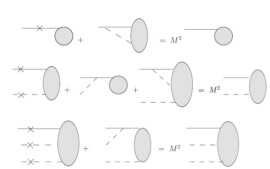
Figure 1: Diagrammatic representation of the first three coupled equations for the wave functions of the dressed-fermion state, Eqs. (10)-(2) in the text. The large blobs represent wave functions, the crosses represent light-cone energies, the solid lines indicate the fermion constituent, and the dashed lines correspond to bosons.

We define the physical wave functions as the coefficients of Fock states containing only particles with positive-definite norm. This reduction can be achieved by requiring all Fock states to be expressed in terms of the positive-norm creation operators $b_{0s}^{\dagger}$ and $a_{0}^{\dagger}$ and the zero-norm combinations $b_{s}^{\dagger}\equiv b_{0s}^{\dagger}+b_{1s}^{\dagger}$ and $a^{\dagger}\equiv a_{0}^{\dagger}+a_{1}^{\dagger}$. We then discard any term containing a $b_{s}^{\dagger}$ or an $a^{\dagger}$, which would be annihilated by the PV-generalized electromagnetic current, leaving the physical state

$$\Phi_{+{\rm phys}}=(z_{0}-z_{1})b_{1+}^{\dagger}(\underline{P})|0\rangle$$

$$+\sum_{s}\int d\underline{q}\left(\sum_{ij}(-1)^{i+j}f_{ijs}(\underline{q})\right)b_{0s}^{\dagger}(\underline{P}-\underline{q})a_{0}^{\dagger}(\underline{q})|0\rangle$$

$$+\sum_{s}\int d\underline{q_{1}}d\underline{q_{2}}\left(\sum_{ijk}\frac{(-1)^{i+j+k}}{\sqrt{1+\delta_{jk}}}f_{ijks}(\underline{q_{1}},\underline{q_{2}})\right)$$

$$\rule{144.54pt}{0.0pt}\times b_{0s}^{\dagger}(\underline{P}-\underline{q_{1}}-\underline{q_{2}})a_{0}^{\dagger}(\underline{q_{1}})a_{0}^{\dagger}(\underline{q_{2}})|0\rangle+\ldots$$

It is normalized by

$$1=(z_{0}-z_{1})^{2}+\sum_{s}\int d\underline{q}\left|\sum_{ij}(-1)^{i+j}f_{ijs}(\underline{q})\right|^{2}$$

$$+\sum_{s}\int d\underline{q_{1}}d\underline{q_{2}}\left|\sum_{ijk}(-1)^{i+j+k}\frac{\sqrt{2}}{\sqrt{1+\delta_{jk}}}f_{ijks}(\underline{q_{1}},\underline{q_{2}})\right|^{2}+\ldots$$

From this state we can compute a boson structure function

$$f_{Bs}(y)=\int d\underline{q}\delta(y-q^{+}/P^{+})\left|\sum_{ij}(-1)^{i+j}f_{ijs}(\underline{q})\right|^{2}$$

$$+\int d\underline{q_{1}}d\underline{q_{2}}\sum_{n=1}^{2}\delta(y-q_{n}^{+}/P^{+})\left|\sum_{ijk}(-1)^{i+j+k}\frac{\sqrt{2}}{\sqrt{1+\delta_{jk}}}f_{ijks}(\underline{q_{1}},\underline{q_{2}})\right|^{2}+\ldots,$$

which is defined as the probability density for finding a constituent boson of longitudinal momentum fraction $y$ when the constituent fermion has helicity $s$. The form factor slope $F^{\prime}_{1}(0)$ is given by [7]

$$F^{\prime}_{1}(0)=-\sum_{s}\int d\underline{q}\left|\frac{y}{2}\vec{\nabla}_{\perp}\sum_{ij}(-1)^{i+j}f_{ijs}(\underline{q})\right|^{2}$$

$$-\sum_{s}\int d\underline{q_{1}}d\underline{q_{2}}\sum_{l}\left|\frac{y_{l}}{2}\vec{\nabla}_{l\perp}\sum_{ijk}(-1)^{i+j+k}\frac{\sqrt{2}}{\sqrt{1+\delta_{jk}}}f_{ijks}(\underline{q_{1}},\underline{q_{2}})\right|^{2}-\ldots,$$

with $\vec{\nabla}_{l\perp}=\hat{x}\frac{\partial}{\partial q_{lx}}+\hat{y}\frac{\partial}{\partial q_{ly}}$. Since no transverse cutoff is used, this expression is no longer the approximation that it was in earlier work [7, 8, 9]. The Dirac radius of the state is given by $R=\sqrt{-6F^{\prime}_{1}(0)}$. From the two-body wave function, we compute a distribution function

$$\phi(x,Q_{\perp})\equiv\int^{Q_{\perp}}\frac{d^{2}k_{\perp}}{\sqrt{16\pi^{3}}}\sum_{ij}(-1)^{i+j}f_{ij+}(1-x,-\vec{k}_{\perp})$$ (17)

and its moments

$$f_{M} \equiv \int_{0}^{1}dx\phi(x,Q_{\perp}),\;\;\bar{x}\equiv\int_{0}^{1}dx\,x\phi(x,Q_{\perp})/f_{M},$$ (18)

$$\bar{x^{2}} \equiv \int_{0}^{1}dx\,x^{2}\phi(x,Q_{\perp})/f_{M}.$$

We can also calculate the axial coupling constant

$$g_{A}=(z_{0}-z_{1})^{2}+\sum_{s}(-1)^{s-1/2}\int d\underline{q}\left|\sum_{ij}(-1)^{i+j}f_{ijs}(\underline{q})\right|^{2}$$

$$+\sum_{s}(-1)^{s-1/2}\int d\underline{q_{1}}d\underline{q_{2}}\left|\sum_{ijk}(-1)^{i+j+k}\frac{\sqrt{2}}{\sqrt{1+\delta_{jk}}}f_{ijks}(\underline{q_{1}},\underline{q_{2}})\right|^{2}+\ldots$$

and the anomalous magnetic moment [25]

$$\kappa=-M\sum_{s}\int d\underline{q}\left(\sum_{ij}(-1)^{i+j}f_{ijs}^{\uparrow*}(\underline{q})\right)y\left(\frac{\partial}{\partial q_{x}}+i\frac{\partial}{\partial q_{y}}\right)\left(\sum_{ij}(-1)^{i+j}f_{ijs}^{\downarrow}(\underline{q})\right)$$

$$-M\sum_{s}\int d\underline{q_{1}}d\underline{q_{2}}\left(\sum_{ijk}(-1)^{i+j+k}\frac{\sqrt{2}}{\sqrt{1+\delta_{jk}}}f_{ijks}^{\uparrow*}(\underline{q_{1}},\underline{q_{2}})\right)$$

$$\rule{36.135pt}{0.0pt}\times\sum_{l}\left[y_{l}\left(\frac{\partial}{\partial q_{lx}}+i\frac{\partial}{\partial q_{ly}}\right)\right]\left(\sum_{ijk}(-1)^{i+j+k}\frac{\sqrt{2}}{\sqrt{1+\delta_{jk}}}f_{ijks}^{\downarrow}(\underline{q_{1}},\underline{q_{2}})\right)$$

$$-\ldots$$

Here an up or down arrow indicates wave functions associated with a dressed fermion having a $J_{z}$ value that is positive or negative, respectively. The wave functions with an up arrow are the same as those without an arrow; the coupled system of equations is constructed and solved for this case. The wave functions for the opposite spin are related as $f_{\ldots\pm}^{\downarrow}=\mp f_{\ldots\mp}^{\uparrow*}$, as can be established by comparing the equations that they each satisfy.

Once the coupled equations are truncated to a finite system, we have a well-defined problem with cancellations of infinities between any infinite integrals. The PV particles are kept in the basis to provide these cancellations. A one-boson truncation produces an analytically solvable problem, which we explored in [11] and discuss briefly here in Sec. 3. Less severe truncations produce larger coupled systems that require numerical techniques for their solution. Given an accurate discretization and the consequent finite matrix eigenvalue problem, one can compute mass eigenvalues and associated wave functions. The bare parameters, i.e. the bare coupling $g$ and the bare mass $m_{0}$ of the positive-norm fermion, can be fixed by fitting “physical” constraints. Here we specify the dressed fermion’s mass $M$ and radius $R$; the fit to a chosen value of $R$ is determined by an iterative root-finding scheme.

The discretization must be chosen carefully. When the PV masses are large, the integrals become sensitive to small momentum fractions, of order $\mu_{0}^{2}/\mu_{1}^{2}$ and $\mu_{0}^{2}/m_{1}^{2}$. This makes traditional DLCQ [14] impractical, because it divides the longitudinal momentum into segments of equal size; the number of segments then grows as $\mu_{1}^{2}/\mu_{0}^{2}$ and $m_{1}^{2}/\mu_{0}^{2}$, making the matrix diagonalization problem impossibly large. We instead employ a discretization based on Gauss–Legendre quadrature and certain variable transformations, as discussed more fully in Sec. 4 and Appendix B. The derivatives needed for computing the radius and the anomalous moment are estimated from cubic-spline fits to $\left[(m_{i}^{2}+q_{\perp}^{2})/(1-y)+(\mu_{j}^{2}+q_{\perp}^{2})/y\right]f_{ijs}(y,q_{\perp})$ as a function of $q_{\perp}$ at fixed $y$. The use of the multiplier reduces the variation in $f$ and makes possible a better fit. Standard finite-difference approximations are not useful, because the quadrature scheme introduces very unequal spacings.

3 One-boson truncation

As an alternative to traditional DLCQ, we can explicitly truncate the system with respect to the total number of bosons in any Fock state. We have already studied the case of the one-boson truncation [11] where the system of two equations can be solved analytically. The structure of the solution is as follows. From the second equation in the system, Eq. (2), the one-boson wave functions are immediately found to be

$$f_{ij+}(\underline{q}) = \frac{P^{+}}{M^{2}-\frac{m_{i}^{2}+q_{\perp}^{2}}{1-q^{+}/P^{+}}-\frac{\mu_{j}^{2}+q_{\perp}^{2}}{q^{+}/P^{+}}}\left[\left\{\sum_{k}(-1)^{k}z_{k}\right\}U_{i}(\underline{P}-\underline{q},\underline{q})\right.$$

$$\rule{144.54pt}{0.0pt}\left.+\sum_{k}(-1)^{k}z_{k}U_{k}(\underline{P},\underline{q})\right],$$

$$f_{ij-}(\underline{q}) = \frac{P^{+}}{M^{2}-\frac{m_{i}^{2}+q_{\perp}^{2}}{1-q^{+}/P^{+}}-\frac{\mu_{j}^{2}+q_{\perp}^{2}}{q^{+}/P^{+}}}\left\{\sum_{k}(-1)^{k}z_{k}\right\}V_{+}^{*}(\underline{P}-\underline{q},\underline{q}).$$ (21)

Substitution into the first equation, Eq. (10), yields algebraic equations for the bare-fermion amplitudes, which are

$$(M^{2}-m_{i}^{2})z_{i} = g^{2}\mu_{0}^{2}(z_{0}-z_{1})J+g^{2}m_{i}(z_{0}m_{0}-z_{1}m_{1})I_{0}$$ (22)

$$+g^{2}\mu_{0}[(z_{0}-z_{1})m_{i}+z_{0}m_{0}-z_{1}m_{1}]I_{1},$$

with

$$I_{n}(M^{2}) = \int\frac{dydq_{\perp}^{2}}{16\pi^{2}}\sum_{jk}\frac{(-1)^{j+k}}{M^{2}-\frac{m_{j}^{2}+q_{\perp}^{2}}{1-y}-\frac{\mu_{k}^{2}+q_{\perp}^{2}}{y}}\frac{(m_{j}/\mu_{0})^{n}}{y(1-y)^{n}},\;\;(n=0,1),$$ (23)

$$J(M^{2}) = \int\frac{dydq_{\perp}^{2}}{16\pi^{2}}\sum_{jk}\frac{(-1)^{j+k}}{M^{2}-\frac{m_{j}^{2}+q_{\perp}^{2}}{1-y}-\frac{\mu_{k}^{2}+q_{\perp}^{2}}{y}}\frac{(m_{j}^{2}+q_{\perp}^{2})/\mu_{0}^{2}}{y(1-y)^{2}}=\frac{M^{2}}{\mu_{0}^{2}}I_{0}.$$ (24)

The presence of the PV regulators makes these integrals finite and allows $I_{0}$ and $J$ to satisfy the identity $\mu_{0}^{2}J(M^{2})=M^{2}I_{0}(M^{2})$. Because $M$ is held fixed, these equations can be viewed as an eigenvalue problem for $g^{2}$. The solution to this eigenvalue problem is

$$g^{2}=-\frac{(M\mp m_{0})(M\mp m_{1})}{(m_{1}-m_{0})(\mu_{0}I_{1}\pm MI_{0})},\;\;\frac{z_{1}}{z_{0}}=\frac{M\mp m_{0}}{M\mp m_{1}}.$$ (25)

Structure functions and distribution amplitudes can then be computed and the PV-mass limits studied. Figures 2, 3, and 4 show typical results. The two-boson contribution is computed perturbatively. The forms show a significant sensitivity to the Pauli–Villars masses.

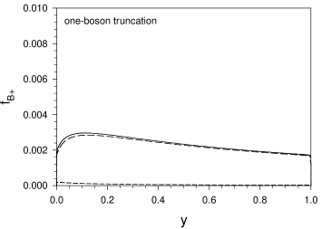
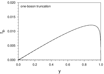
(a)	(b)
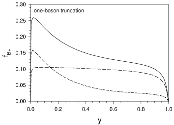
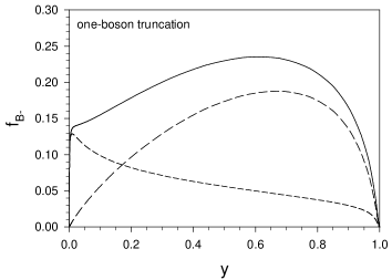
(c)	(d)

Figure 2: Bosonic structure functions $f_{B\pm}(y)$ as defined in Eq. (2) of the text, where $y=x_{B}=q^{+}/P^{+}$, for the dressed-fermion state with mass $M=\mu_{0}$ and radius $R=0.01/\mu_{0}$. The wave functions are computed from a truncation to one constituent boson, with the two-boson contribution then computed perturbatively. The solid line includes both contributions. The long dashes show the one-boson contribution, and the short dashes show the two-boson contribution. For (a) and (b), the PV masses are $m_{1}=\mu_{1}=2000\mu_{0}$, and for (c) and (d), they are $m_{1}=50000\mu_{0}$ and $\mu_{1}=500\mu_{0}$.

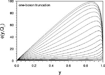
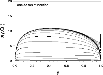
(a)	(b)

Figure 3: Same as Fig. 2 but for the distribution amplitude $\phi(x,Q_{\perp})$ defined in Eq. (17) of the text. The individual lines correspond to different values of $Q_{\perp}$. For (a) the PV masses are $m_{1}=\mu_{1}=2000\mu_{0}$, and for (b) they are $m_{1}=50000\mu_{0}$ and $\mu_{1}=500\mu_{0}$.

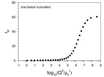
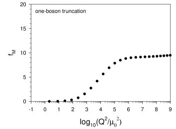
(a)	(b)
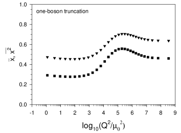
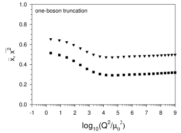
(c)	(d)

Figure 4: Moments of the distribution function, as defined in Eq. (18) of the text. The filled circles correspond to $f_{M}$, the triangles to $\bar{x}$, and the squares to $\bar{x^{2}}$. For (a) and (c), the PV masses are $m_{1}=\mu_{1}=2000\mu_{0}$, and for (b) and (d), they are $m_{1}=50000\mu_{0}$ and $\mu_{1}=500\mu_{0}$.

Further results can be found in Ref. [11].

4 Two-boson truncation

4.1 Effective equations

For a two-boson truncation, the solution is no longer analytic, but the coupled equations (10)-(2) can be reduced to eight equations for the two-particle amplitudes only, which are of the form

$$\left[M^{2}-\frac{m_{i}^{2}+q_{\perp}^{2}}{1-y}-\frac{\mu_{j}^{2}+q_{\perp}^{2}}{y}\right]f_{ijs}(y,q_{\perp})=\frac{g^{2}}{16\pi^{2}}\sum_{a}\frac{I_{ija}(y,q_{\perp})}{1-y}f_{ajs}(y,q_{\perp})$$

$$+\frac{g^{2}}{16\pi^{2}}\sum_{abs^{\prime}}\int_{0}^{1}dy^{\prime}dq_{\perp}^{\prime 2}J_{ijs,abs^{\prime}}^{(0)}(y,q_{\perp};y^{\prime},q^{\prime}_{\perp})f_{abs^{\prime}}(y^{\prime},q^{\prime}_{\perp})$$

$$+\frac{g^{2}}{16\pi^{2}}\sum_{abs^{\prime}}\int_{0}^{1-y}dy^{\prime}dq_{\perp}^{\prime 2}J_{ijs,abs^{\prime}}^{(2)}(y,q_{\perp};y^{\prime},q^{\prime}_{\perp})f_{abs^{\prime}}(y^{\prime},q^{\prime}_{\perp}),$$

with the angular dependence removed via $\sqrt{P^{+}}f_{ij+}(\underline{q})=f_{ij+}(y,q_{\perp})$ and $\sqrt{P^{+}}f_{ij-}(\underline{q})=f_{ij-}(y,q_{\perp})e^{i\phi}$. Here $I_{ija}$ is a computable self-energy and $J_{ijs,abs^{\prime}}^{(n)}$ is the kernel due to $n$-boson intermediate states. Specific forms for $I$ and $J^{(n)}$ can be found in Appendix A. A diagrammatic representation is given in Fig. 5.

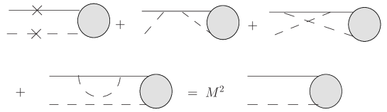
Figure 5: Same as Fig. 1 but for the effective equations in (4.1) of the text.

There is a difficulty with the structure of this eigenvalue problem, because the original eigenvalue $M^{2}$ appears in the denominator of integrands that go into finding the matrix elements. If attacked directly, this nonlinearity requires an additional layer of numerical effort, to get a self-consistent solution. An indirect approach is to again convert the problem to one where $g^{2}$ is the eigenvalue. To maintain symmetry (up to the indefinite norm), this conversion is done by defining a new function

$$\tilde{f}_{ij\pm}=f_{ij\pm}\sqrt{\frac{m_{i}^{2}+q_{\perp}^{2}}{1-y}+\frac{\mu_{j}^{2}+q_{\perp}^{2}}{y}-M^{2}}$$ (27)

before completing the rearrangement. The smallest real $g$ that is obtained for a given $M$ is taken to be the coupling value for which $M$ is the mass of the lowest state. Obviously, this works well with the renormalization condition where $M$ is fixed as input.

4.2 Method of solution

We solve the reduced integral equations (4.1) numerically by converting them to a discrete matrix equation via Gauss–Legendre quadrature of the integrals. The resolution of the quadrature is characterized by the order of the underlying polynomial, which we denote by $K$ in the longitudinal direction and by $2N+1$ in the transverse direction. For the transverse quadrature, only odd orders are used, to keep $q_{\perp}=0$ as a quadrature point, and only $N+1$ points are used. (The other $N$ points correspond to negative $q_{\perp}$.) Thus $K$ and $N$ characterize the resolution of the approximation, and we consider large values in order to be close to the continuum limit.

Before applying the quadrature rules, the variables $y^{\prime}$ and $q^{\prime}_{\perp}$ are transformed in such a way as to emphasize those regions most important to the approximation. In the case of $q^{\prime}_{\perp}$, the transformation is chosen also to produce a finite range of integration without introduction of a cutoff. Since the PV contributions make the integrals finite, no cutoff is needed for the continuum problem, and any cutoff would only be an artifact of the numerical approximation if introduced. A more complete discussion of the transformations is given in Appendix B.

The matrix eigenvalue problem is solved by applying the Lanczos diagonalization scheme developed previously [9]. This particular scheme was designed to efficiently handle the present situation where the matrix is self-adjoint with respect to an indefinite norm. What is different here, compared to the case in [9], is that the matrix is not sparse. Nevertheless, the Lanczos approach is much faster than standard diagonalization algorithms for nonsymmetric matrices, because we are interested in only one eigenstate. Typical matrix sizes are on the order of 20,000 by 20,000, but provide as many nonzero entries as the much larger sparse matrices considered in [9].

Use of the Lanczos technique is important for another reason. Standard diagonalization routines have difficulty when there are multiple mass scales in the problem; specifically, when $\mu_{1}$ is intermediate between $\mu_{0}$ and $m_{1}$, such that $\mu_{0}\ll\mu_{1}\ll m_{1}$, the standard diagonalization can fail. For the Lanczos process, we need only an accurate representation of the product of the matrix and a vector. The contribution of $J^{(0)}$ to the matrix can then be written in a factorized form $\sum_{i^{\prime}=0}^{1}(-1)^{i^{\prime}}\vec{v}_{i^{\prime}}\vec{v}_{i^{\prime}}^{T}\eta/(M^{2}-m_{i^{\prime}}^{2})$, where $\eta$ is a diagonal matrix that represents the signature of the norm, as determined by the factors $(-1)^{a+b}$ given as part of the definition of $J^{(0)}$ in Eq. (29). This factorized form provides a more faithful numerical representation of the contribution from $J^{(0)}$ by restricting the $J^{(0)}$-vector product to a linear combination of the vectors $\vec{v}_{i^{\prime}}$.

4.3 Results

The convergence with resolution is indicated in Fig. 6.

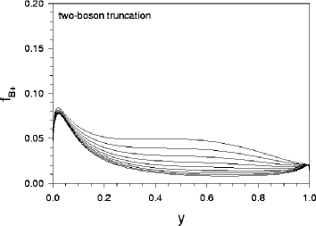
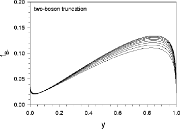
(a)	(b)
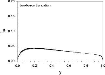
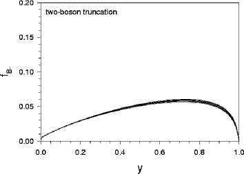
(c)	(d)

Figure 6: Bosonic structure functions $f_{B\pm}(y)$, as defined in Eq. (2) of the text, for the dressed-fermion state with mass $M=\mu_{0}$. The wave functions are computed from a truncation to two constituent bosons. The longitudinal resolution is varied from $K=30$ to $K=70$, with the transverse resolution fixed at $N=30$. The bare coupling is $g=2$. For (a) and (b) the PV masses are $m_{1}=\mu_{1}=1000\mu_{0}$, and for (c) and (d) they are $m_{1}=10000\mu_{0}$ and $\mu_{1}=100\mu_{0}$. In (a) the amplitude of $f_{B+}$ decreases with increasing $K$, and in (b) the amplitude of $f_{B-}$ increases.

For most quantities, and for the range of PV masses considered, resolutions of $K=50$ and $N=30$ are sufficient for convergence, and we use these resolutions for most of our calculations.

The variation of the structure functions and some characteristic quantities with respect to PV mass can be seen in Figs. 7, 8, and 9.

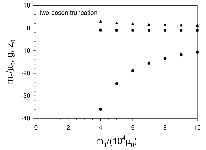
Figure 7: The bare mass $m_{0}$ of the constituent fermion (filled circles), the bare coupling $g$ (triangles), and the bare-fermion amplitude $z_{0}$ (squares) as functions of the PV fermion mass $m_{1}$. The ratio $\mu_{1}/m_{1}$ of PV boson mass to fermion mass is fixed at 0.01. The dressed mass is $M=\mu_{0}$, the radius is $R=0.01/\mu_{0}$, and the numerical resolutions are $K=50$ and $N=30$.

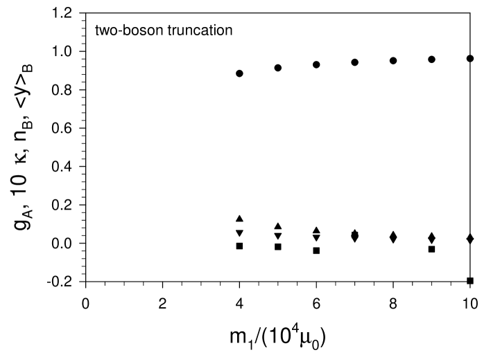
Figure 8: Same as Fig. 7 but for the axial coupling $g_{A}$ (filled circles), the anomalous moment $\kappa$ (squares), the average number of bosons $n_{B}$ (upward triangles), and the average momentum fraction $\langle y\rangle_{B}$ (downward triangles).

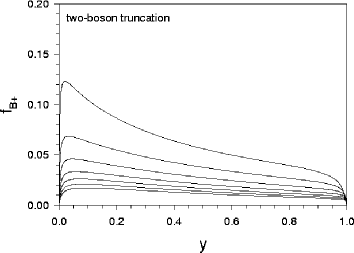
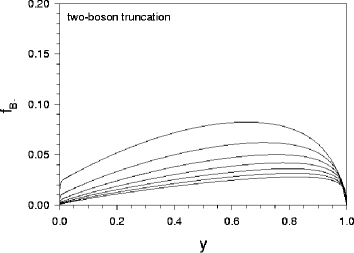
(a)	(b)

Figure 9: Bosonic structure functions $f_{B\pm}$ for the dressed-fermion state with mass $M=\mu_{0}$ and radius $R=0.01/\mu_{0}$. The different curves correspond to increasing values of $m_{1}$. The ratio $\mu_{1}/m_{1}$ is fixed at 0.01. The numerical resolutions are $K=50$ and $N=30$.

When the PV masses are equal, the radius of the state with mass $M=\mu_{0}$ is driven to zero as the PV mass is made large; thus in this limiting case a fixed radius cannot be maintained. The distribution amplitude and its moments are shown in Figs. 10 and 11 for two sets of PV masses.

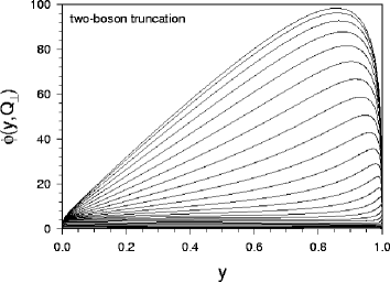
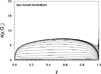
(a)	(b)

Figure 10: Same as Fig. 3 but for the two-boson truncation.

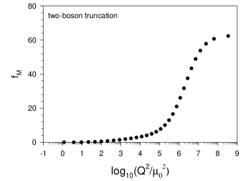
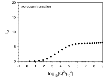
(a)	(b)
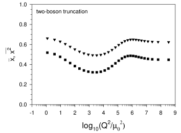
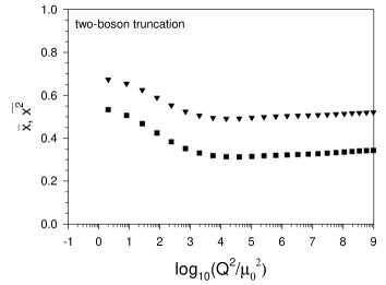
(c)	(d)

Figure 11: Same as Fig. 4 but for the two-boson truncation.

A comparison of results for the one and two-boson truncations at fixed resolution and fixed PV masses is given in Figs. 12 and 13. The dressed-fermion radius $R$ is held fixed at the same value of $0.01/\mu_{0}$ for both truncations. The one and two-boson contributions to the structure functions are shown in Fig. 14; these should be compared with the results in Fig. 2 for the one-boson truncation. To see the comparison more easily, the one and two-boson contributions in each case are plotted separately in Figs. 15 and 16. The differences in the results, between the one-boson and two-boson truncations, reflects not only the effects of including the two-boson contributions to the kernel in the one-boson equation, but also the differences in the bare fermion mass and the bare coupling. In the case of unequal PV masses, as in Figs. 15(c) and (d) and 16(c) and (d), the perturbative calculation significantly overestimates the two-boson contribution.

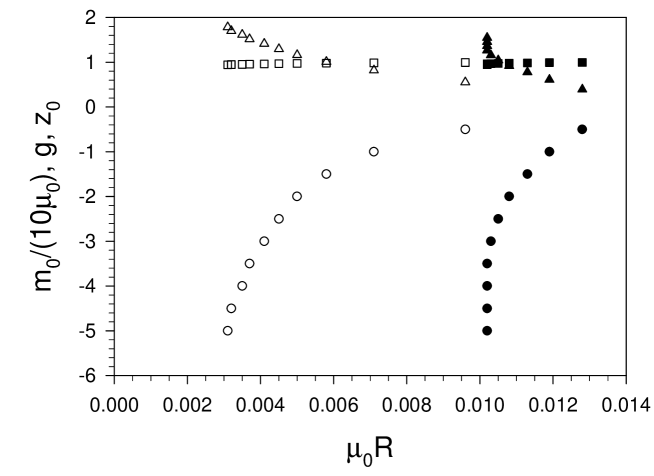
(a)

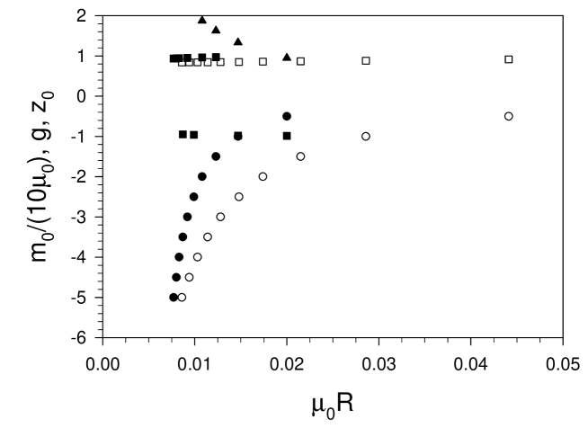
(b)

Figure 12: The bare fermion mass $m_{0}$ (circles), the Yukawa coupling $g$ (triangles), and the bare fermion amplitude $z_{0}$ (squares) as functions of the radius $R$. For (a) the PV masses are $m_{1}=\mu_{1}=2000\mu_{0}$, and for (b) they are $m_{1}=50000\mu_{0}$ and $\mu_{1}=500\mu_{0}$. The filled symbols correspond to the two-boson truncation, and the open symbols to the one-boson truncation. The dressed-fermion mass is $M=\mu_{0}$, and the resolutions are $K=50$ and $N=30$. For the one-boson truncation, the two-boson contribution is computed perturbatively.

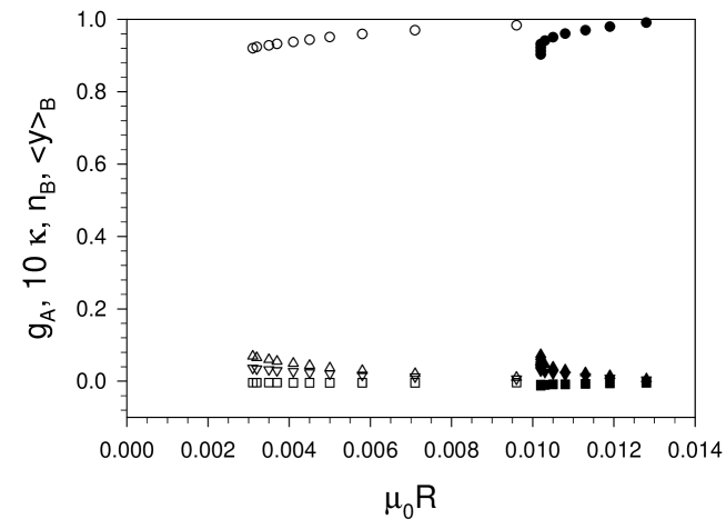
(a)

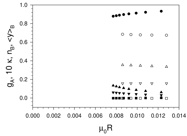
(b)

Figure 13: Same as Fig. 12 but for the axial coupling $g_{A}$ (circles), the anomalous moment $\kappa$ (squares), the average number of bosons $n_{B}$ (upward triangles), and the average momentum fraction $\langle y\rangle_{B}$ (downward triangles). The filled symbols correspond to the two-boson truncation, and the open symbols to the one-boson truncation.

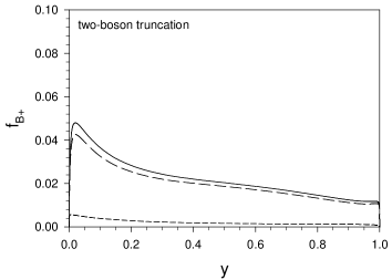
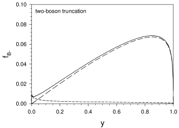
(a)	(b)
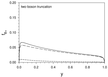
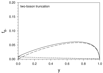
(c)	(d)

Figure 14: Same as Fig. 2 but for the wave functions computed from a truncation to two constituent bosons instead of one, with the bare coupling $g$ and bare-fermion mass $m_{0}$ adjusted to maintain $M=\mu_{0}$ and $R=0.01/\mu_{0}$. The resolutions are $K=50$ and $N=30$.

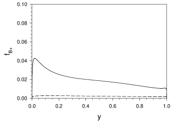
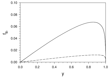
(a)	(b)
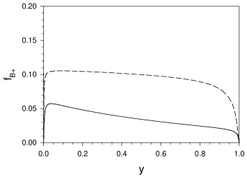
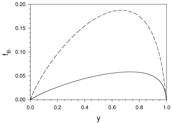
(c)	(d)

Figure 15: One-boson contributions to the structure functions $f_{B\pm}(y)$ as computed in the one-boson (dashed) and two-boson (solid) truncations. The dressed-fermion mass is $M=\mu_{0}$, and the radius is $R=0.01/\mu_{0}$. For (a) and (b), the PV masses are $m_{1}=\mu_{1}=2000\mu_{0}$, and for (c) and (d), they are $m_{1}=50000\mu_{0}$ and $\mu_{1}=500\mu_{0}$. The two-boson truncation is calculated with resolutions $K=50$ and $N=30$.

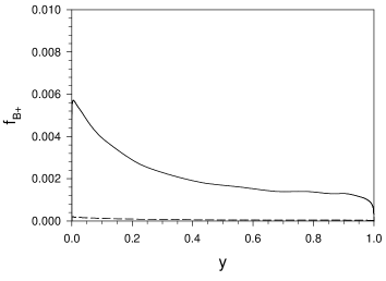
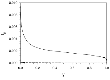
(a)	(b)
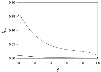
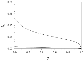
(c)	(d)

Figure 16: Same as Fig. 15, but for the two-boson contribution. In the case of the one-boson truncation, this is computed perturbatively.

In principle, these solutions can be used to estimate the optimal PV mass for the one-boson truncation. As the PV masses are increased, we expect the PV contributions to the one-boson Fock sector to decrease, but the magnitude of the total contribution from the two-boson sector to increase. The latter measures the truncation error for a one-boson calculation that does not include two-boson states even perturbatively. (To estimate the optimal PV mass for a two-boson truncation, we would need to estimate the three-boson contribution, which would require a much larger calculation.) These two measures, the PV contribution to the probability of the one-boson sector, $e_{1}$, and the ratio of the total probability of the two-boson sector to that of the one-boson sector, $e_{2}$, are plotted in Fig. 17, along with $e_{2}^{\rm pert}$, a perturbative estimate of $e_{2}$. We compute $e_{1}$ as the ratio of the PV contribution to the physical contribution, each of which is individually divergent but regulated by a transverse cutoff at $q_{\perp}^{2}=(3\mu_{1})^{2}$. The fermion mass is held fixed but very large. The optimal PV boson mass would be chosen to make the two errors equal; this apparently corresponds to a mass on the order of $250\mu_{0}$.

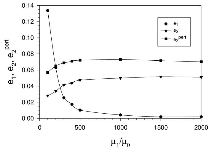
Figure 17: Measures of error in the truncations used as functions of the PV boson mass $\mu_{1}$. The quantity $e_{1}$ is a measure of the PV contribution to the probability of the one-boson sector, and $e_{2}$ is a measure of the truncation error, defined as the ratio of the total probability of the two-boson sector to that of the one-boson sector. The latter is computed both in the two-boson truncation and perturbatively in the one-boson truncation. The PV fermion mass is fixed at a large value, $m_{1}=50000\mu_{0}$, and the coupling is fixed at $g=2$. The bare fermion mass $m_{0}$ is allowed to vary, to maintain the constraint of $M^{2}=\mu_{0}^{2}$ on the dressed-fermion mass. The dressed-fermion radius is allowed to vary. The resolutions are $K=50$ and $N=30$.

5 Discussion

We have solved for the dressed fermion state in Yukawa theory using Pauli–Villars regularization and a truncation to no more than one fermion and two bosons in the Fock expansion. The solution yields the bare coupling $g$, the bare mass $m_{0}$ of the constituent fermion, and the Fock-state wave functions as functions of the PV masses $\mu_{1}$ and $m_{1}$ and the dressed mass $M$ and radius $R$. A limited region of the parameter space has been explored; however, a wide range of PV mass values was studied in order to observe the limiting behavior as these masses approached infinity. We also studied the effects of truncation by comparing the solutions obtained previously with no more than one boson in the basis.

From the wave functions, we calculated various properties of the dressed fermion. These are shown in Figs. 12 and 13. The one and two-boson truncations agree in the weak-coupling, large-radius limit, as expected, but show significant differences for stronger coupling, even though a two-boson contribution is included perturbatively in the case of the one-boson truncation. The presence of the two-boson intermediate states in the kernel of the effective integral equation does have important effects.

The use of light-cone quantization, Pauli–Villars regularization, and carefully crafted quadrature schemes can produce accurate solutions for bound states in quantum field theory. These techniques should be applicable to more interesting situations, such as the dressed electron in quantum electrodynamics [12] and two-fermion bound states in Yukawa theory and QED. As applications to a gauge theory become better understood, we can hope to develop methods sufficiently robust to solve for the bound states of quantum chromodynamics.

Appendix A: Interaction kernels

The self-energy in the reduced, coupled system Eq. (4.1) is

$$I_{ija} = \sum_{i^{\prime},b}(-1)^{i^{\prime}+a+b}(1-y)\int_{0}^{1-y}\frac{dy^{\prime}}{y^{\prime}}\frac{d\phi^{\prime}}{2\pi}dq_{\perp}^{\prime 2}\frac{-1}{D_{i^{\prime}jb}+F\cos\phi^{\prime}}$$

$$\times\left[\left(\frac{m_{i^{\prime}}}{1-y-y^{\prime}}+\frac{m_{i}}{1-y}\right)\left(\frac{m_{i^{\prime}}}{1-y-y^{\prime}}+\frac{m_{a}}{1-y}\right)\right.$$

$$\left.+\frac{1}{(1-y-y^{\prime})^{2}}\left(\frac{y^{\prime 2}q_{\perp}^{2}}{(1-y)^{2}}+q_{\perp}^{\prime 2}+\frac{2y^{\prime}q_{\perp}q^{\prime}_{\perp}\cos\phi^{\prime}}{(1-y)}\right)\right].$$

The bare-fermion kernel is

$$J_{ij+,ab+}^{(0)} = \sum_{i^{\prime}}\frac{(-1)^{i^{\prime}+a+b}}{\sqrt{yy^{\prime}}}\frac{1}{M^{2}-m_{i^{\prime}}^{2}}\left(\frac{m_{i}}{1-y}+m_{i^{\prime}}\right)\left(\frac{m_{a}}{1-y^{\prime}}+m_{i^{\prime}}\right),$$ (29)

$$J_{ij+,ab-}^{(0)} = \sum_{i^{\prime}}\frac{(-1)^{i^{\prime}+a+b}}{\sqrt{yy^{\prime}}}\frac{1}{M^{2}-m_{i^{\prime}}^{2}}\left(\frac{m_{i}}{1-y}+m_{i^{\prime}}\right)\frac{q^{\prime}_{\perp}}{1-y^{\prime}},$$

$$J_{ij-,ab+}^{(0)} = \sum_{i^{\prime}}\frac{(-1)^{i^{\prime}+a+b}}{\sqrt{yy^{\prime}}}\frac{1}{M^{2}-m_{i^{\prime}}^{2}}\frac{q_{\perp}}{1-y}\left(\frac{m_{a}}{1-y^{\prime}}+m_{i^{\prime}}\right),$$

$$J_{ij-,ab-}^{(0)} = \sum_{i^{\prime}}\frac{(-1)^{i^{\prime}+a+b}}{\sqrt{yy^{\prime}}}\frac{1}{M^{2}-m_{i^{\prime}}^{2}}\frac{q_{\perp}}{1-y}\frac{q^{\prime}_{\perp}}{1-y^{\prime}},$$

and the two-boson kernel is

$$J_{ij+,ab+}^{(2)} = \sum_{i^{\prime}}\frac{(-1)^{i^{\prime}+a+b}}{\sqrt{yy^{\prime}}}\int\frac{d\phi^{\prime}}{2\pi}\frac{-1}{D_{i^{\prime}jb}+F\cos\phi^{\prime}}$$

$$\times\left(\left[\frac{m_{i^{\prime}}}{1-y-y^{\prime}}+\frac{m_{a}}{1-y^{\prime}}\right]\left[\frac{m_{i^{\prime}}}{1-y-y^{\prime}}+\frac{m_{i}}{1-y}\right]\right.$$

$$+\frac{1}{(1-y-y^{\prime})^{2}}\left[\frac{y^{\prime}q_{\perp}^{2}}{1-y}+\frac{yq_{\perp}^{\prime 2}}{1-y^{\prime}}\right.$$

$$\left.\left.\rule{90.3375pt}{0.0pt}+\frac{(1-y-y^{\prime}+2yy^{\prime})q_{\perp}q^{\prime}_{\perp}}{(1-y)(1-y^{\prime})}\cos\phi^{\prime}\right]\right),$$

$$J_{ij+,ab-}^{(2)} = \sum_{i^{\prime}}\frac{(-1)^{i^{\prime}+a+b}}{\sqrt{yy^{\prime}}}\int\frac{d\phi^{\prime}}{2\pi}\frac{-1}{D_{i^{\prime}jb}+F\cos\phi^{\prime}}$$

$$\times\left(-\left[\frac{m_{i^{\prime}}}{1-y-y^{\prime}}+\frac{m_{i}}{1-y}\right]\frac{yq^{\prime}_{\perp}}{(1-y-y^{\prime})(1-y^{\prime})}\right.$$

$$+\left[\frac{m_{i^{\prime}}}{1-y-y^{\prime}}+\frac{m_{a}}{1-y^{\prime}}\right]\frac{q^{\prime}_{\perp}}{1-y-y^{\prime}}$$

$$-\left[\frac{m_{i^{\prime}}}{1-y-y^{\prime}}+\frac{m_{i}}{1-y}\right]\frac{q_{\perp}\cos\phi^{\prime}}{1-y-y^{\prime}}$$

$$\left.+\left[\frac{m_{i^{\prime}}}{1-y-y^{\prime}}+\frac{m_{a}}{1-y^{\prime}}\right]\frac{y^{\prime}q_{\perp}\cos\phi^{\prime}}{(1-y-y^{\prime})(1-y)}\right),$$

$$J_{ij-,ab+}^{(2)} = \sum_{i^{\prime}}\frac{(-1)^{i^{\prime}+a+b}}{\sqrt{yy^{\prime}}}\int\frac{d\phi^{\prime}}{2\pi}\frac{-1}{D_{i^{\prime}jb}+F\cos\phi^{\prime}}$$

$$\times\left(-\left[\frac{m_{i^{\prime}}}{1-y-y^{\prime}}+\frac{m_{a}}{1-y^{\prime}}\right]\frac{y^{\prime}q_{\perp}}{(1-y-y^{\prime})(1-y)}\right.$$

$$+\left[\frac{m_{i^{\prime}}}{1-y-y^{\prime}}+\frac{m_{i}}{1-y}\right]\frac{q_{\perp}}{1-y-y^{\prime}}$$

$$-\left[\frac{m_{i^{\prime}}}{1-y-y^{\prime}}+\frac{m_{a}}{1-y^{\prime}}\right]\frac{q^{\prime}_{\perp}\cos\phi^{\prime}}{1-y-y^{\prime}}$$

$$\left.+\left[\frac{m_{i^{\prime}}}{1-y-y^{\prime}}+\frac{m_{i}}{1-y}\right]\frac{yq^{\prime}_{\perp}\cos\phi^{\prime}}{(1-y-y^{\prime})(1-y^{\prime})}\right),$$

$$J_{ij-,ab-}^{(2)} = \sum_{i^{\prime}}\frac{(-1)^{i^{\prime}+a+b}}{\sqrt{yy^{\prime}}}\int\frac{d\phi^{\prime}}{2\pi}\frac{-1}{D_{i^{\prime}jb}+F\cos\phi^{\prime}}$$

$$\times\left(\left[\frac{m_{i^{\prime}}}{1-y-y^{\prime}}+\frac{m_{a}}{1-y^{\prime}}\right]\left[\frac{m_{i^{\prime}}}{1-y-y^{\prime}}+\frac{m_{i}}{1-y}\right]\cos\phi^{\prime}\right.$$

$$+\frac{1}{(1-y-y^{\prime})^{2}}\left[\frac{y^{\prime}q_{\perp}^{2}}{1-y}+\frac{yq_{\perp}^{\prime 2}}{1-y^{\prime}}\right]\cos\phi^{\prime}$$

$$\left.-\frac{q_{\perp}q^{\prime}_{\perp}}{(1-y-y^{\prime})(1-y)(1-y^{\prime})}+\frac{2q_{\perp}q^{\prime}_{\perp}\cos^{2}\phi^{\prime}}{(1-y-y^{\prime})^{2}}\right).$$

Here we have used

$$D_{ijk} = \frac{m_{i}^{2}+q_{\perp}^{2}+q_{\perp}^{\prime 2}}{1-y-y^{\prime}}+\frac{\mu_{j}^{2}+q_{\perp}^{2}}{y}+\frac{\mu_{k}^{2}+q_{\perp}^{\prime 2}}{y^{\prime}}-M^{2},$$ (34)

$$F = \frac{2q_{\perp}q^{\prime}_{\perp}}{1-y-y^{\prime}},$$

as well as a shift in the azimuthal angle $\phi^{\prime}-\phi\rightarrow\phi^{\prime}$. The angular integrals can be done analytically; they are

$$\int_{0}^{2\pi}\frac{d\phi^{\prime}}{2\pi}\frac{1}{D+F\cos\phi^{\prime}} = \frac{1}{\sqrt{D^{2}-F^{2}}},$$ (35)

$$\int_{0}^{2\pi}\frac{d\phi^{\prime}}{2\pi}\frac{\cos\phi^{\prime}}{D+F\cos\phi^{\prime}} = \frac{1}{F}\left(1-\frac{D}{\sqrt{D^{2}-F^{2}}}\right),$$ (36)

$$\int_{0}^{2\pi}\frac{d\phi^{\prime}}{2\pi}\frac{\cos^{2}\phi^{\prime}}{D+F\cos\phi^{\prime}} = -\frac{D}{F^{2}}\left(1-\frac{D}{\sqrt{D^{2}-F^{2}}}\right).$$ (37)

The integrals in the self-energy $I_{ija}$ also can be done analytically. After a change of variables to $\xi=q^{\prime+}/q^{+}=y^{\prime}/(1-y)$ and $\vec{k}_{\perp}=\vec{q}_{\perp}^{\,\prime}+\xi\vec{q}_{\perp}$, we obtain

$$I_{ija} = -\sum_{i^{\prime},b}(-1)^{i^{\prime}+a+b}\int_{0}^{1}\frac{d\xi}{\xi}\frac{d^{2}k_{\perp}}{\pi}\frac{m_{i}m_{a}+\frac{m_{i}+m_{a}}{1-\xi}m_{i^{\prime}}+\frac{m_{i}^{\prime 2}+k_{\perp}^{2}}{(1-\xi)^{2}}}{M_{j}^{2}+\frac{m_{i^{\prime}}^{2}+k_{\perp}^{2}}{1-\xi}+\frac{\mu_{b}^{2}+k_{\perp}^{2}}{\xi}}$$

$$= 16\pi^{2}(-1)^{a}\left[m_{i}m_{a}I_{0}(-M_{j}^{2})+\mu_{0}(m_{i}+m_{a})I_{1}(-M_{j}^{2})+\mu_{0}^{2}J(-M_{j}^{2})\right],$$

with

$$M_{j}^{2}\equiv\frac{\mu_{j}^{2}+q_{\perp}^{2}}{y}-\mu_{j}^{2}-(1-y)M^{2}>0,$$ (39)

and $I_{0}$, $I_{1}$, and $J$ defined in Eqs. (23) and (24). For $J$ we have $\mu_{0}^{2}J(-M_{j}^{2})=-M_{j}^{2}I_{0}(-M_{j}^{2})$. For $I_{0}$ and $I_{1}$, integration over $\vec{k}_{\perp}$ yields

$$16\pi^{2}I_{0} = \sum_{i^{\prime}b}(-1)^{i^{\prime}+b}(L_{0i^{\prime}b}-L_{1i^{\prime}b}),$$ (40)

$$16\pi^{2}I_{1} = \sum_{i^{\prime}b}(-1)^{i^{\prime}+b}\frac{m_{i^{\prime}}}{\mu_{0}}L_{0i^{\prime}b},$$ (41)

where

$$L_{ni^{\prime}b}\equiv\int_{0}^{1}dzz^{n}\ln[zm_{i^{\prime}}^{2}/M_{j}^{2}+(1-z)\mu_{b}^{2}/M_{j}^{2}+z(1-z)].$$ (42)

Integration over $z$ obtains

$$L_{0i^{\prime}b} = (1-y_{ji^{\prime}b})\ln\left(\frac{m_{i^{\prime}}^{2}}{M_{j}^{2}}\right)+y_{ji^{\prime}b}\ln\left(\frac{\mu_{b}^{2}}{M_{j}^{2}}\right)-2$$

$$-\sqrt{x_{ji^{\prime}b}}\ln\left[\frac{\sqrt{x_{ji^{\prime}b}}+y_{ji^{\prime}b}-1}{\sqrt{x_{ji^{\prime}b}}-y_{ji^{\prime}b}+1}\frac{\sqrt{x_{ji^{\prime}b}}-y_{ji^{\prime}b}}{\sqrt{x_{ji^{\prime}b}}+y_{ji^{\prime}b}}\right],$$

$$L_{1i^{\prime}b} = y_{ji^{\prime}b}L_{0i^{\prime}b}-\frac{1}{2}\left[\frac{m_{i^{\prime}}^{2}}{M_{j}^{2}}\ln\left(\frac{m_{i^{\prime}}^{2}}{M_{j}^{2}}\right)-\frac{m_{i^{\prime}}^{2}}{M_{j}^{2}}-\frac{\mu_{b}^{2}}{M_{j}^{2}}\ln\left(\frac{\mu_{b}^{2}}{M_{j}^{2}}\right)+\frac{\mu_{b}^{2}}{M_{j}^{2}}\right],$$ (44)

with $y_{ji^{\prime}b}\equiv(m_{i^{\prime}}^{2}-\mu_{b}^{2}+M_{j}^{2})/(2M_{j}^{2})$ and $x_{ji^{\prime}b}\equiv y_{ji^{\prime}b}^{2}+\mu_{b}^{2}/M_{j}^{2}$.

In practice one needs to use an alternate form when $M_{j}^{2}$ is small, as happens when $q_{\perp}^{2}$ is zero and $y$ is near 1. This alternate form is obtained as an expansion in powers of $M_{j}^{2}$ of the integrand in (42), written as

$$L_{ni^{\prime}b}=\int_{0}^{1}dzz^{n}\ln[zm_{i^{\prime}}^{2}+(1-z)\mu_{b}^{2}+M_{j}^{2}z(1-z)]-\frac{\ln\left(M_{j}^{2}\right)}{n+1}.$$ (45)

The dependence on $\ln\left(M_{j}^{2}\right)$ cancels in the sums in (40) and (41). When $M_{j}^{2}z(1-z)/\left(zm_{i^{\prime}}^{2}+(1-z)\mu_{b}^{2}\right)$ is of order 0.01 or smaller at $z=1/2$, two-term expansions of the first term in (45) in powers of $M_{j}^{2}$ are sufficient as replacements for (Appendix A: Interaction kernels) and (44).

There is also a special form needed when $M_{j}^{2}$ is large, such as when $z$ is near zero. When $M_{j}^{2}$ is greater than $10m_{1}^{2}$ or $10\mu_{1}^{2}$, expansions of the analytic expressions (Appendix A: Interaction kernels) and (44) to order $\mu_{0}^{2}/M_{j}^{2}$ and $\ln(M_{j}/\mu_{0})\mu_{0}^{2}/M_{j}^{2}$ are used.

Appendix B: Quadrature schemes

To solve the integral equations (4.1), we convert them to a matrix equation via quadrature in $y^{\prime}$ and $q_{\perp}^{\prime 2}$ and then diagonalize the matrix. For integrals with an upper limit of $y^{\prime}=1-y$, the form of the integrand at $1-y$ is obtained by explicitly taking the limit; the PV counterterms insure that this limit is finite. The quadrature weight is reduced by 1/2 at that point, to take into account the edge effect.

A particularly useful set of quadrature schemes is based on Gauss–Legendre quadrature combined with variable transformations to allocate quadrature points to important regions and to reduce the $q_{\perp}^{\prime 2}$ integral to a finite range. The transformations for the $y^{\prime}$ integral are

$$y^{\prime}(t) = t^{3}(1+dt)/[1+d-(3+4d)t+(3+6d)t^{2}-4dt^{3}+2dt^{4}],$$ (46)

$$t(u) = 2u-1.$$ (47)

The new variable $u$ ranges between -1 and 1, which is the nominal range for Gauss–Legendre quadrature. The transformation from $y^{\prime}$ to $t$ is motivated by the need for an accurate approximation to the integral $J$, defined in (24). This integral is largely determined by contributions near the endpoints whenever the PV masses are large. The transformation $y^{\prime}(t)$ places many of the quadrature points near 0 and 1. It was found empirically, beginning with a transformation constructed to compute the integral $\int[\ln(y+\epsilon_{0})-\ln(y+\epsilon_{1})]dy$ exactly from the quadrature formula, with $\epsilon_{0}$ and $\epsilon_{1}$ small. The final form is restricted to be symmetric under the transformation $t\rightarrow(1-t)$. The parameter $d$ is chosen such that $y^{\prime}\simeq 0.01t^{3}$ for small $t$.

For the transverse integral, the transformation is

$$q_{\perp}^{\prime 2}(v)=a^{2}\frac{1-\left(b^{2}/a^{2}\right)^{v}}{\left(b^{2}/a^{2}\right)^{v-1}-1},$$ (48)

with $v$ in the range 0 to 1. Only the positive Gauss–Legendre quadrature points of an odd order are used for $v$ between -1 and 1, so that $v=0$, and therefore $q^{\prime}_{\perp}=0$, is always a quadrature point. The points in the negative half of the range are discarded. To maintain the accuracy of the underlying sum, the weight of the point at zero is reduced by a factor of 1/2. The transformation from $q_{\perp}^{\prime 2}$ to $v$ is motivated by its ability to obtain an exact result for the integral $\int[1/(a^{2}+q^{2})-1/(b^{2}+q^{2})]dq^{2}$. For use in the integral equation (4.1), the parameters $a$ and $b$ are chosen to be the smallest and largest mass scales, i.e. $a=\mu_{0}$ and $b=m_{1}$.

References

• [1] R.J. Perry, A. Harindranath, and K.G. Wilson, Phys. Rev. Lett. 65 (1990), 2959.
• [2] R.J. Perry and K.G. Wilson, Nucl. Phys. B 403 (1993), 587.
• [3] St.D. Głazek and K.G. Wilson, Phys. Rev. D 49 (1994), 4214.
• [4] C.J. Burden, L. Qian, C.D. Roberts, P.C. Tandy, and M.J. Thomson, Phys. Rev. C 55 (1997), 2649 [arXiv:nucl-th/9605027].
• [5] P.C. Tandy, Nucl. Phys. B (Proc. Suppl.) 141 (2005), 9 [arXiv:nucl-th/0408037].
• [6] K.G. Wilson, Nucl. Phys. B (Proc. Suppl.) 140 (2005), 3.
• [7] S.J. Brodsky, J.R. Hiller, and G. McCartor, Phys. Rev. D 58 (1998), 025005 [arXiv:hep-th/9802120].
• [8] S.J. Brodsky, J.R. Hiller, and G. McCartor, Phys. Rev. D 60 (1999), 054506 [arXiv:hep-ph/9903388].
• [9] S.J. Brodsky, J.R. Hiller, and G. McCartor, Phys. Rev. D 64 (2001), 114023 [arXiv:hep-ph/0107038].
• [10] S.J. Brodsky, J.R. Hiller, and G. McCartor, Ann. Phys. 296 (2002), 406 [arXiv:hep-th/0107246].
• [11] S.J. Brodsky, J.R. Hiller, and G. McCartor, Ann. Phys. 305 (2003), 266 [arXiv:hep-th/0209028].
• [12] S.J. Brodsky, V.A. Franke, J.R. Hiller, G. McCartor, S.A. Paston, and E.V. Prokhvatilov, Nucl. Phys. B 703 (2004), 333 [arXiv:hep-ph/0406325].
• [13] W. Pauli and F. Villars, Rev. Mod. Phys. 21 (1949), 4334.
• [14] H.-C. Pauli and S.J. Brodsky, Phys. Rev. D 32 (1985), 1993; 32 (1985), 2001.
• [15] S.J. Brodsky, H.-C. Pauli, and S.S. Pinsky, Phys. Rep. 301 (1997), 299 [arXiv:hep-ph/9705477].
• [16] S.A. Paston and V.A. Franke, Theor. Math. Phys.  112 (1997), 1117 [Teor. Mat. Fiz. 112 (1997), 399] [arXiv:hep-th/9901110].
• [17] S.A. Paston, V.A. Franke, and E.V. Prokhvatilov, Theor. Math. Phys.  120 (1999), 1164 [Teor. Mat. Fiz. 120 (1999), 417] [arXiv:hep-th/0002062].
• [18] P.A.M. Dirac, Rev. Mod. Phys. 21 (1949), 392.
• [19] A.B. Bylev, S.D. Głazek, and J. Przeszowski, Phys. Rev. C 53 (1996), 3097.
• [20] D. Bernard, Th. Cousin, V.A. Karmanov, and J.-F. Mathiot, Phys. Rev. D 65 (2002), 025016.
• [21] M. Mangin-Brinet, J. Carbonell, and V.A. Karmanov, Phys. Rev. C 68 (2003), 055203.
• [22] St.D. Głazek and T. Maslowski, Phys. Rev. D 65 (2002), 065011; St.D. Głazek and M. Wieckowski, Phys. Rev. D 66 (2002), 016001; St.D. Głazek and J. Mlynik, Phys. Rev. D 67 (2003), 045001.
• [23] O. Lunin and S. Pinsky, in New Directions in Quantum Chromodynamics, edited by C.-R. Ji and D.-P. Min, AIP Conf. Proc. No. 494 (AIP, Melville, NY, 1999), p. 140 [hep-th/9910222]; J.R. Hiller, S.S. Pinsky, and U. Trittmann, Phys. Rev. D 67 (2003), 115005 [arXiv:hep-ph/0304147]; Nucl. Phys. B 661 (2003), 99 [arXiv:hep-ph/0302119]; J.R. Hiller, Y. Proestos, S. Pinsky, and N. Salwen, Phys. Rev. D 70 (2004), 065012 [arXiv:hep-th/0407076]; M. Harada, J.R. Hiller, S. Pinsky, and N. Salwen, Phys. Rev. D 70 (2004), 045015 [arXiv:hep-th/0404123].
• [24] M. Burkardt and S. Dalley, Prog. Part. Nucl. Phys.  48 (2002) 317 [arXiv:hep-ph/0112007]; S. Dalley and B. van de Sande, Phys. Rev. D 67 (2003), 114507.
• [25] S.J. Brodsky and S.D. Drell, Phys. Rev. D 22 (1980), 2236.