Higgs Production in Association with Bottom Quarks at Hadron Colliders

Abstract

We review the present status of the QCD corrected cross sections and kinematic distributions for the production of a Higgs boson in association with bottom quarks at the Fermilab Tevatron and CERN Large Hadron Collider. Results are presented for the Minimal Supersymmetric Standard Model where, for large $\tan\beta$, these production modes can be greatly enhanced compared to the Standard Model case. The next-to-leading order QCD results are much less sensitive to the renormalization and factorization scales than the lowest order results, but have a significant dependence on the choice of the renormalization scheme for the bottom quark Yukawa coupling. We also investigate the uncertainties coming from the Parton Distribution Functions and find that these uncertainties can be comparable to the uncertainties from the remaining scale dependence of the next-to-leading order results. We present results separately for the different final states depending on the number of bottom quarks identified.

I Introduction

One of the most exciting prospects of particle physics is the discovery of the source of Electroweak Symmetry Breaking (EWSB). In the Standard Model (SM), a single $SU(2)_{L}$ complex scalar doublet is responsible for both gauge boson masses (via the Higgs mechanism) and fermion masses (via Yukawa interactions). The only scalar physical remnant of the process is the Higgs boson ($h$) whose mass is a free parameter of the model. In contrast, the Minimal Supersymmetric Standard Model (MSSM) contains two complex $SU(2)_{L}$ scalar doublets, as required to give masses to both up- and down-type quarks and to cancel gauge anomalies. Once EWSB occurs in the MSSM, the scalar sector contains five physical Higgs bosons: a light scalar $h^{0}$, a heavy scalar $H^{0}$, a pseudoscalar $A^{0}$ and a pair of charged bosons $H^{\pm}$. Finding experimental evidence for the existence of one or more Higgs bosons is, thus, a major goal of current and future collider experiments. In addition, measuring the couplings of the Higgs boson(s) to gauge bosons, leptons and quarks would be imperative to uncover the true structure of the Higgs sector.

Direct searches for Higgs bosons at LEP2 have placed lower mass limits on both the SM Higgs ($M_{h}>$ 114.4 GeV at $95\%$ c.l.) Barate:2003sz and the lightest scalar and pseudoscalar Higgs bosons of the MSSM ($M_{h^{0},A^{0}}{\stackrel{{\scriptstyle>}}{{\scriptstyle\sim}}}$ 93 GeV at $95\%$ c.l.) Lephwg2:2004 . In addition, the mass of the lightest scalar Higgs boson of the MSSM is also bounded from above by theory to less than $\sim$ 130 GeV. Finally, precision electroweak measurements, which are sensitive to the effects of Higgs boson loop contributions, imply that the mass of the SM Higgs boson should be less than $\sim$ 186 GeV at $95\%$ c.l. Lepewwg:2004 ($\sim$ 219 GeV when including the LEP-2 direct search limit). Hence, in both the SM and the MSSM, a Higgs boson should lie in a mass range which can be explored at the Large Hadron Collider (LHC) Carena:2002es .

The dominant production mechanism for a SM Higgs boson in hadronic interactions ($p\bar{p}$ or $pp$) is gluon fusion ($gg\rightarrow h$), which proceeds predominantly through a loop of top quarks. Among the production modes with smaller rates, the associated production with electroweak gauge bosons ($q\bar{q}\rightarrow Vh$, where $V=W^{\pm},Z^{0}$) or with top quark pairs ($q\bar{q},gg\rightarrow t\bar{t}h$), as well as weak boson fusion ($qq\rightarrow qqh$), play crucial roles. The next-to-leading order (NLO) QCD corrections have been calculated for all of the above processes  Han:1991ia ; Han:1992hr ; Dawson:1991zj ; Djouadi:1991tk ; Graudenz:1993 ; Spira:1995 ; Beenakker:2001rj ; Reina:2001sf ; Reina:2001bc ; Beenakker:2002nc ; Dawson:2002tg ; Dawson:2003zu , while for gluon fusion and associated $Vh$ production corrections are also known at next-to-next-to-leading order (NNLO) in perturbative QCD Harlander:2002wh ; Anastasiou:2002yz ; Harlander:2003ai ; Catani:2001ic ; Ravindran:2002dc ; Brein:2003wg .

In the MSSM, the hierarchy of production modes can be significantly different from that of the SM. In fact, for large values of $\tan\beta$ (the ratio of the two MSSM Higgs vacuum expectation values), the bottom quark Yukawa couplings to both scalar and pseudoscalar Higgs bosons become strongly enhanced and the production of Higgs bosons with bottom quarks dominates over all other production modes.

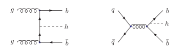
Figure 1: Sample Feynman diagrams for $gg\rightarrow b\bar{b}h$ and $q\bar{q}\rightarrow b\bar{b}h$ production at tree level.

Recently, the production of Higgs bosons in association with bottom quarks has received much interest from both the theoretical and experimental communities Campbell:2004 ; Avto:2005 ; Acosta:2005bk . At tree level, the cross section is almost entirely dominated by the sub-process $gg\rightarrow b\bar{b}h$, with only a small contribution from $q\bar{q}\rightarrow b\bar{b}h$, at both the Tevatron and LHC (see Fig. 1). The theoretical prediction of $b\bar{b}h$ production at hadron colliders, however, involves several subtle issues, as will be described in detail in this review, and depends on the number of bottom quarks identified, or tagged, in the final state. In case of no or only one tagged bottom quark there are two approaches available for calculating the cross sections to $b\bar{b}h$ production, dubbed the four flavor (4FNS) and five flavor (5FNS) number schemes. The main difference between these two approaches is that the 4FNS is a fixed-order calculation of QCD corrections to the $gg,q\bar{q}$-induced $b\bar{b}h$ production processes, while in the 5FNS the leading processes are induced by $bg$ ($\bar{b}g$) and $b\bar{b}$ initial states and large collinear logarithms present at tree level as well as at each order of QCD corrections are resummed by using a pertubatively defined bottom quark Parton Distribution Function (PDF). The two schemes are described in more detail in Section II.2 and II.1, respectively.

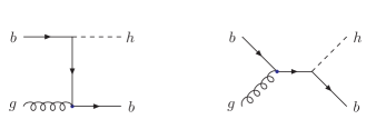
Figure 2: Tree level Feynman diagram for $bg\rightarrow bh$ in the 5FNS.

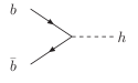
Figure 3: Tree level Feynman diagram for $b\bar{b}\rightarrow h$ in the 5FNS.

For purposes of differentiating the final states, we introduce the following terminology. Exclusive $b\bar{b}h$ production refers to the case when both bottom quark jets are tagged (or are at high transverse momentum, $p_{T}$). Note that, in this case, the computation of the cross section solely relies on the 4FNS. Semi-inclusive production (denoted by $b(\bar{b})h$) pertains to the case when at least one bottom quark is at high $p_{T}$. Here, the dominant leading-order (LO) process for the 4FNS (5FNS) is $gg\rightarrow b(\bar{b})h$ ($bg\rightarrow bh$ or $\bar{b}g\rightarrow\bar{b}h$, see Fig. 2). Finally, the inclusive production process (denoted by $(b\bar{b})h$) involves the case where no bottom quark jets are tagged. The dominant LO process for this mode is $gg\rightarrow(b\bar{b})h$ ($b\bar{b}\rightarrow h$, see Fig. 3) in the 4FNS (5FNS). It should be mentioned that, although the cross section for the inclusive production mode dominates over the less inclusive modes by one to two orders of magnitude, tagging bottom quark jets greatly reduces backgrounds, making the less inclusive modes experimentally more appealing. Requiring one or two high-$p_{T}$ bottom quark jets in the final state also ensures that the detected Higgs boson has been radiated off a bottom or anti-bottom quark and the corresponding cross section is unambiguously proportional to the bottom quark Yukawa coupling.

QCD corrected cross sections are available for all three final states and the inclusive and semi-inclusive production processes have been computed in both the 4FNS and 5FNS. For the inclusive case, the NLO QCD corrected 4FNS Dittmaier:2003ej ; Campbell:2004 and the NNLO QCD corrected 5FNS cross sections Harlander:2003ai have been compared and are found to be in good agreement within theoretical uncertainties. The NLO predictions of the semi-inclusive cross sections for the 4FNS Dittmaier:2003ej ; Dawson:2004tl and 5FNS Campbell:2002zm have also been extensively compared Campbell:2004 ; Dawson:2004tl and the agreement between the two is spectacular. The compatibility of these two seemingly different calculational schemes in the prediction of inclusive and semi-inclusive Higgs boson production rates is indeed a powerful check of the theory. The 4FNS and 5FNS represent different perturbative expansions of the same physical observables, and therefore should agree at sufficiently high order. Indeed, we see that considering the first (second) order of corrections already brings agreement between the two schemes within the respective theoretical uncertainties. Finally, two independent calculations of the NLO QCD corrections for the exclusive mode have been compared and agreement has been found Dittmaier:2003ej ; Dawson:2003ex ; Campbell:2004 .

The above discussion for the production of a scalar Higgs boson with bottom quarks applies equally well to the production of a pseudoscalar Higgs boson. In fact, for massless bottom quarks, the predictions for $b\bar{b}A^{0}$ would be identical to those of $b\bar{b}h^{0}/H^{0}$ given a rescaling of the Yukawa couplings. For massive bottom quarks, however, the situation becomes complicated due to the $\gamma_{5}$ appearing in the $b\bar{b}A^{0}$ Yukawa coupling. The $\gamma_{5}$ Dirac matrix is intrinsically a four-dimensional object and care must be taken in its treatment when dimensionally regularizing the calculation. In any case, bottom quark mass effects are expected to be small, i.e. $\mathcal{O}$$(\frac{m_{b}^{2}}{M_{h}^{2}})$, and predictions for $b\bar{b}h^{0}/H^{0}$ are good indicators for $b\bar{b}A^{0}$ production (modulus Yukawa couplings).

The remainder of this paper is organized as follows. In Section II, we discuss the framework of the calculations in the four- and five-flavor-number schemes in detail. Given the importance it plays in the prediction of the cross section through the Yukawa coupling, we also discuss different renormalization schemes of the bottom quark mass. Section III details the SUSY-corrected Yukawa couplings obtained from the program FeynHiggs Heinemeyer:2001qd ; Frank:2002qa ; Heinemeyer:2004ms that were used in this study to produce results for MSSM Higgs bosons. In Section IV, we review the results for inclusive, semi-inclusive and exclusive Higgs boson production with bottom quarks. In Section V, we investigate the uncertainties arising from the PDFs for the semi-inclusive $b\bar{b}h$ production process. These uncertainties are calculated using the algorithm developed by the CTEQ collaboration CTEQ:2002 . Finally, we summarize and conclude in Section VI.

II Theoretical Framework

II.1 Five Flavor Number Scheme

Final state bottom quarks are identified imposing cuts on their transverse momentum ($p_{T}\!>\!p_{T}^{min}$) and pseudorapidity ($|\eta|\!<\!\eta^{max}$). On the other hand, when a final state bottom quark is not identified, as in the inclusive and semi-inclusive $b\bar{b}h$ production processes, the corresponding integration over its phase space may give rise to large logarithms of the form:

$$\Lambda_{b}\equiv\ln\left(\frac{\mu^{2}}{m_{b}^{2}}\right)\,\,\,,$$ (1)

where $m_{b}$ and $\mu$ represent the lower and upper bounds on the integration over the transverse momentum, $p_{T}$, of the final state bottom quark. This happens when the final state bottom quark is directly originating from the $g\rightarrow b\bar{b}$ splitting of an initial state gluon, and corresponds to the collinear singularity that would be present in the case of a gluon splitting into massless quarks. The scale $\mu$ is typically of $\mathcal{O}(M_{h})$ and therefore, due to the smallness of the bottom quark mass, these logarithms can be quite large. Additionally, the same logarithms appear at every order in the perturbative expansion of the cross section in the strong coupling, $\alpha_{s}$, due to recursive gluon emission from internal bottom quark lines. These logarithms could severely hinder the convergence of the perturbative expansion of the total and differential cross sections. In the 5FNS the convergence is improved by introducing a perturbatively defined bottom quark PDF Barnett:1988 ; Olness:1988 ; Dicus:1989 , defined at lowest order in $\alpha_{s}$ as

$$b(x,\mu)=\frac{\alpha_{s}(\mu)}{2\pi}\Lambda_{b}\int_{x}^{1}\frac{dy}{y}P_{qg}\left(\frac{x}{y}\right)g(y,\mu)\,\,\,,$$ (2)

where $g(y,\mu)$ is the (experimentally-measured) gluon PDF and $P_{qg}$ is the Altarelli-Parisi splitting function for $g\rightarrow q\bar{q}$ given by

$$P_{qg}(z)=\frac{1}{2}[z^{2}+(1-z)^{2}]\,\,\,.$$ (3)

Subsequently, the $\Lambda_{b}$ logarithms are resummed through the DGLAP evolution equation Gribov:1972 ; Altarelli:1977zs ; Dokshitzer:1977 , such that contributions proportional to $(\alpha_{s}\Lambda_{b})^{n}$ can be absorbed, to all orders in $n$, into a leading logarithms bottom quark PDF, while subleading logarithms are recursively resummed when higher order corrections are considered in the DGLAP equation. Since $\alpha_{s}\Lambda_{b}$ is not a small expansion parameter, the use of a bottom quark PDF should improve the stability of the total and differential cross sections for inclusive and semi-inclusive Higgs boson production with bottom quarks.

The 5FNS is based on the approximation that any spectator bottom quarks (i.e., bottom quarks which are not tagged in the final state) are at small transverse momentum, since this is the region where the $\Lambda_{b}$ logarithms dominate over other $p_{T}$-dependent contributions. At lowest order, the spectator quarks are produced with zero $p_{T}$, and a transverse momentum spectrum for the outgoing bottom quarks is generated at higher orders Barnett:1988 ; Olness:1988 .

With the use of a bottom quark PDF, the 5FNS effectively reorders the perturbative expansion to be one in $\alpha_{s}$ and $\Lambda_{b}^{-1}$. To see how this works, let us consider the perturbative expansion of the inclusive process $b\bar{b}\rightarrow h$ (Fig. 3), which is at tree level of order $\alpha_{s}^{2}\Lambda_{b}^{2}$. At NLO, the virtual and real corrections to the tree level process make contributions of $\mathcal{O}(\alpha_{s}^{3}\Lambda_{b}^{2})$. However, at NLO, we must also consider the contribution from $bg\rightarrow bh$ where the final state bottom quark is at high $p_{T}$. This process makes a contribution of order $\alpha_{s}^{2}\Lambda_{b}$ and is, thus, a correction of $\mathcal{O}(\Lambda_{b}^{-1})$ to the tree level cross section. Similarly, at NNLO, among the myriad of radiative corrections of $\mathcal{O}(\alpha_{s}^{4}\Lambda_{b}^{2})$, we must also include the contribution from the process $gg\rightarrow b\bar{b}h$, where both $b$ and $\bar{b}$ are at high $p_{T}$. The contribution from these diagrams are of order $\alpha_{s}^{2}$, and are, thus, $\mathcal{O}(\Lambda_{b}^{-2})$ (or NNLO) corrections to the tree level process $b\bar{b}\rightarrow h$ Dicus:1989 ; Dicus:1998hs .

The above discussion for $b\bar{b}\rightarrow h$ also applies to the perturbative expansion of $bg\rightarrow bh$. In this case, the tree level process is of order $\alpha_{s}^{2}\Lambda_{b}$ and the contribution from $gg\rightarrow b\bar{b}h$ is a NLO correction of ${\cal{O}}(\Lambda_{b}^{-1})$ Campbell:2002zm .

Finally, we observe that, in the existing 5FNS calculations, all bottom quark masses other than the one appearing in the Yukawa coupling are set to zero.

II.2 Four Flavor Number Scheme

In the 4FNS, the initial state quarks are constrained to be the four lightest quarks, i.e. there are no bottom quarks in the initial state. No kinematic approximations are made and the cross section for $p\bar{p}(pp)\rightarrow b\bar{b}h$ is computed at fixed order in QCD without resumming higher-order collinear logarithms. Moreover, the bottom quark mass is always considered to be non-zero. Similarly to the 5FNS, for the less inclusive final states discussed above ($b(\bar{b})h$ or $b\bar{b}h$), identification cuts are imposed on the final state bottom quark(s) which constrain its transverse momentum and pseudorapidity. Applying these cuts to a final state bottom quark eliminates large logarithms that may appear from gluon splitting and it ensures that the bottom quark jets can be tagged experimentally. While the inclusive and semi-inclusive production of a Higgs boson with bottom quarks can be calculated in both the 4FNS and 5FNS, the exclusive production can only be calculated in the 4FNS, since both final state bottom quarks are tagged.

The NLO QCD corrections to the hadronic process $p\bar{p}(pp)\rightarrow b\bar{b}h$ in the 4FNS consist of calculating the $\mathcal{O}(\alpha_{s})$ virtual and real QCD corrections to the tree level (partonic) processes $q\bar{q},gg\rightarrow b\bar{b}h$ Dittmaier:2003ej ; Dawson:2003ex . We note that the NLO calculation of $p\bar{p}(pp)\rightarrow b\bar{b}h$ is identical to the calculation of the NLO QCD corrections to $p\bar{p}(pp)\rightarrow t\bar{t}h$ Beenakker:2001rj ; Reina:2001sf ; Reina:2001bc ; Beenakker:2002nc ; Dawson:2002tg , with the global interchange of the top quark and bottom quark masses ($m_{t}\leftrightarrow m_{b}$).

II.3 Definition of the bottom quark mass

One potential source of theoretical uncertainty in the calculation of $p\bar{p}(pp)\rightarrow b\bar{b}h$ involves the renormalization of the bottom quark mass. The bottom quark mass counterterm has to be used twice in the renormalization of the calculation: once to renormalize the bottom quark mass appearing in internal propagators and once to renormalize the SM bottom quark Yukawa coupling $g_{b\bar{b}h}^{\scriptscriptstyle S\!M}\!=\!m_{b}/v$, where $v=(\sqrt{2}G_{F})^{-1/2}=246$ GeV. Indeed, if one only considers QCD corrections, the counterterm for the bottom quark Yukawa coupling coincides with the counterterm for the bottom quark mass, since the vacuum expectation value $v$ is not renormalized at 1-loop in QCD.

The renormalization scheme dependence has been studied in Ref. Dawson:2003ex , in the 4FNS, for the case of the exclusive $b\bar{b}h$ production. Two schemes for the renormalization of the bottom quark mass have been chosen: the $\overline{MS}$ scheme and an on-shell ($OS$) scheme. The two are perturbatively consistent at NLO with the only difference being at higher orders and, thus, part of the theoretical uncertainty of the NLO calculation. The main reason for investigating this renormalization scheme dependence is the large sensitivity of the $\overline{MS}$ bottom quark mass and the prominent role it plays in the $b\bar{b}h$ production cross section through the overall bottom quark Yukawa coupling. A summary of the results of this investigation are presented in Section IV.3.

The benefit of using the $\overline{MS}$ scheme for the Yukawa coupling is that it potentially gives control over higher-order corrections beyond the 1-loop corrections. This is often reflected in the better perturbative behavior of physical observables calculated using the $\overline{MS}$ bottom quark Yukawa coupling. Therefore, unless otherwise stated all the results presented in this review are given using the $\overline{MS}$ scheme for the bottom quark mass and Yukawa coupling. This is accomplished by replacing the $\overline{MS}$ bottom quark mass in the Yukawa coupling with the corresponding 1-loop and 2-loop renormalization group improved $\overline{MS}$ masses:

$${\overline{m}}_{b}(\mu)_{1l}=m_{b}\left[\frac{\alpha_{s}(\mu)}{\alpha_{s}(m_{b})}\right]^{c_{0}/b_{0}}\,\,\,,$$ (4)

$${\overline{m}}_{b}(\mu)_{2l}=m_{b}\left[\frac{\alpha_{s}(\mu)}{\alpha_{s}(m_{b})}\right]^{c_{0}/b_{0}}\left[1+\frac{c_{0}}{b_{0}}(c_{1}-b_{1})\frac{\alpha_{s}(\mu)-\alpha_{s}(m_{b})}{\pi}\right]\left(1-\frac{4}{3}\frac{\alpha_{s}(m_{b})}{\pi}\right)\,\,\,,$$ (5)

where we take the bottom quark pole mass to be $m_{b}\!=\!4.62$ GeV and

$$b_{0} =\frac{1}{4\pi}(\frac{11}{3}N-\frac{2}{3}n_{lf})\,\,\,,\,\,\, c_{0}=\frac{1}{\pi}\,\,\,,$$

$$b_{1} =\frac{1}{2\pi}\frac{51N-19n_{lf}}{11N-2n_{lf}}\,\,\,, c_{1}=\frac{1}{72\pi}(101N-10n_{lf})$$ (6)

are the one and two loop coefficients of the QCD $\beta$ function and mass anomalous dimension $\gamma_{m}$, while $N=3$ is the number of colors and $n_{lf}=5$ is the number of light flavors.

III Radiatively-corrected MSSM bottom Yukawa Coupling

So far, most of the results for $b\bar{b}h$ production have been obtained in the SM, in order to simplify the comparison of different calculations and approaches (for a review see, e.g., Ref. Campbell:2004 ). As stated earlier, though, these processes are relevant discovery modes at hadron colliders only for SUSY models with large $\tan\beta$. Therefore, we will present most of the following results for the case of the MSSM with large $\tan\beta$. The prediction for the MSSM case can easily be derived from the SM results by rescaling the Yukawa couplings. In the 4FNS, due to the existence of diagrams where the Higgs is radiated off a closed top quark loop, some care must be taken when performing this rescaling. In this review, all 4FNS results for the neutral MSSM Higgs bosons, are obtained from the SM results by carefully rescaling the contributions with ($\sigma_{\scriptscriptstyle S\!M}$) and without top quark loops ($\sigma_{\scriptscriptstyle S\!M}-\sigma_{\scriptscriptstyle S\!M}^{t}$) as:

$$\sigma_{\scriptscriptstyle M\!S\!S\!M} = \left(\frac{g_{b\bar{b}h}^{\scriptscriptstyle M\!S\!S\!M}}{g_{b\bar{b}h}^{\scriptscriptstyle S\!M}}\right)^{2}\left(\sigma_{\scriptscriptstyle S\!M}-\sigma_{\scriptscriptstyle S\!M}^{t}\right)+\left(\frac{g_{t\bar{t}h}^{\scriptscriptstyle M\!S\!S\!M}g_{b\bar{b}h}^{\scriptscriptstyle M\!S\!S\!M}}{g_{t\bar{t}h}^{\scriptscriptstyle S\!M}g_{b\bar{b}h}^{\scriptscriptstyle S\!M}}\right)\sigma_{\scriptscriptstyle S\!M}^{t}\,\,\,.$$ (7)

Examples of the closed top quark loop contributions described by $\sigma_{\scriptscriptstyle S\!M}^{t}$ are shown in Fig. 4. Note that in the 5FNS, as implemented in the program MCFM MCFM:2004 , the corresponding contributions to $\sigma_{\scriptscriptstyle S\!M}^{t}$ are considered to be zero. While this could affect the comparison in the SM, in SUSY models with large bottom quark Yukawa couplings (and consequently small top quark Yukawa couplings) the contributions of the closed top quark diagrams is very small, and $\sigma_{\scriptscriptstyle S\!M}^{t}$ does not play a significant role.

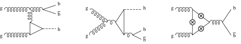
Figure 4: Sample Feynman diagrams for the closed top quark loop contribution to $gg\rightarrow b\bar{b}h$. The circled cross denotes all possible insertion of the final state Higgs boson leg, each insertion corresponding to a different diagram.

In the MSSM the bottom and top quark Yukawa couplings to the scalar, neutral Higgs bosons are given by:

$$\begin{array}[]{lclrcr}g_{b\bar{b}h^{0}}^{\scriptscriptstyle M\!S\!S\!M}&=&-\displaystyle{\frac{\sin\alpha}{\cos\beta}}g_{b\bar{b}h}^{\scriptscriptstyle S\!M}\,\,\,,&g_{t\bar{t}h^{0}}^{\scriptscriptstyle M\!S\!S\!M}&=&\displaystyle{\frac{\cos\alpha}{\sin\beta}}g_{t\bar{t}h}^{\scriptscriptstyle S\!M}\,\,\,,\\ g_{b\bar{b}H^{0}}^{\scriptscriptstyle M\!S\!S\!M}&=&\displaystyle{\frac{\cos\alpha}{\cos\beta}}g_{b\bar{b}h}^{\scriptscriptstyle S\!M}\,\,\,,&g_{t\bar{t}H^{0}}^{\scriptscriptstyle M\!S\!S\!M}&=&\displaystyle{\frac{\sin\alpha}{\sin\beta}}g_{t\bar{t}h}^{\scriptscriptstyle S\!M}\,\,\,,\end{array}$$ (8)

where $g_{b\bar{b}h}^{\scriptscriptstyle S\!M}$ and $g_{t\bar{t}h}^{\scriptscriptstyle S\!M}$ are the SM bottom and top quark Yukawa couplings, $h^{0}$ and $H^{0}$ are the lighter and heavier neutral scalars of the MSSM, and $\alpha$ is the angle which diagonalizes the neutral scalar Higgs mass matrix Gunion:1989we . The dominant SUSY radiative corrections to $b\bar{b}h$ production can be taken into account by including the SUSY corrections to the $b\bar{b}h$ vertex only, i.e. by replacing the tree level Yukawa couplings by the radiative corrected ones. We follow the treatment of the program FeynHiggs FeynHiggs:2005 and take into account the leading, $\tan\beta$ enhanced, radiative corrections that are generated by gluino-sbottom and chargino-stop loops, as follows Carena:1999py :

$$g_{b\bar{b}h^{0}}^{\scriptscriptstyle M\!S\!S\!M} = -g_{b\bar{b}h}^{\scriptscriptstyle S\!M}\frac{1}{1+\Delta_{b}}\left[\frac{\sin\alpha}{\cos\beta}-\Delta_{b}\frac{\cos\alpha}{\sin\beta}\right]\,\,\,,$$

$$g_{b\bar{b}H^{0}}^{\scriptscriptstyle M\!S\!S\!M} = \,\,\,\,g_{b\bar{b}h}^{\scriptscriptstyle S\!M}\frac{1}{1+\Delta_{b}}\left[\frac{\cos\alpha}{\cos\beta}+\Delta_{b}\frac{\sin\alpha}{\sin\beta}\right]\,\,\,,$$ (9)

with

$$\Delta_{b} = \mu\tan\beta\left[\frac{2\alpha_{s}(m_{t})}{3\pi}M_{\tilde{g}}I(m_{\tilde{b}_{1}},m_{\tilde{b}_{2}},m_{\tilde{g}})+\left(\frac{h_{t}}{4\pi}\right)^{2}A_{t}I(m_{\tilde{t}_{1}},m_{\tilde{t}_{2}},\mu)\right]\,\,\,,$$ (10)

where $h_{t}=\overline{m}_{t}(m_{t})/\sqrt{v_{1}^{2}+v_{2}^{2}}\approx\overline{m}_{t}(m_{t})/174$ GeV, $m_{\tilde{b}_{1,2}},m_{\tilde{t}_{1,2}},M_{\tilde{g}}$ denote the sbottom, stop, and gluino masses, respectively, $A_{t}$ is the stop and $\mu$ the Higgs mixing parameter. The strong coupling constant and the running top quark mass, $\overline{m}_{t}$, are evaluated at the on-shell top mass, $m_{t}\!=\!174$ GeV. The vertex function $I$ is given by

$$I(a,b,c) = \frac{[a^{2}b^{2}\ln(\frac{a^{2}}{b^{2}})+b^{2}c^{2}\ln(\frac{b^{2}}{c^{2}})+a^{2}c^{2}\ln(\frac{c^{2}}{a^{2}})]}{(a^{2}-b^{2})(b^{2}-c^{2})(a^{2}-c^{2})}\,\,\,.$$ (11)

In Tables 1 and 2 we provide the ratios of the SM and MSSM bottom and top quark Yukawa couplings at $\tan\beta\!=\!40$, as provided by FeynHiggs, where we assumed CP conserving couplings . In the following, we will use these ratios to derive the MSSM cross sections from the SM results as described in Eq. (7). Using FeynHiggs, the MSSM Higgs boson masses and the mixing angle $\alpha$ have been computed up to two-loop order. As expected, for this choice of MSSM input parameters the bottom Yukawa coupling is strongly enhanced and the top Yukawa coupling is suppressed, resulting in a MSSM $b\bar{b}h$ cross section that is about three orders of magnitude larger than the SM cross section.

$\tan\beta=40$
$M_{h^{0}}$ [GeV]	100	110	120	130
$\alpha$ [rad]	-1.5063	-1.4716	-1.3798	-0.7150
$g_{b\bar{b}h^{0}}^{\scriptscriptstyle M\!S\!S\!M}/g_{b\bar{b}h}^{\scriptscriptstyle S\!M}$	33.913	33.823	33.387	22.390
$g_{t\bar{t}h^{0}}^{\scriptscriptstyle M\!S\!S\!M}/g_{t\bar{t}h}^{\scriptscriptstyle S\!M}$	0.0645	0.0991	0.1899	0.7553

Table 1: Ratios of the MSSM and SM bottom and top quark Yukawa couplings to a light neutral scalar, along with the corresponding values for $\alpha$ as computed by FeynHiggs FeynHiggs:2005 . The genuine SUSY input parameters are chosen as follows: all soft-SUSY breaking masses for squark doublets and singlets are set to $M_{SUSY}\!=\!1$ TeV, $M_{\tilde{g}}\!=\!1$ TeV, $A_{b}\!=\!A_{t}\!=\!2$ TeV, and $\mu\!=\!M_{2}\!=\!200$ GeV. For this choice we find $\Delta_{b}\!=\!0.178$.

$\tan\beta=40$
$M_{H^{0}}$ [GeV]	120	200	300	400	500	600	800
$\alpha$ [rad]	-0.3315	-0.0454	-0.0318	-0.0282	-0.0266	-0.0258	-0.0251
$g_{b\bar{b}H^{0}}^{\scriptscriptstyle M\!S\!S\!M}/g_{b\bar{b}h}^{\scriptscriptstyle S\!M}$	25.787	27.338	27.356	27.360	27.362	27.363	27.364
$g_{t\bar{t}H^{0}}^{\scriptscriptstyle M\!S\!S\!M}/g_{t\bar{t}h}^{\scriptscriptstyle S\!M}$	-0.3255	-0.0454	-0.0318	-0.0282	-0.0266	-0.0258	-0.0251

Table 2: Ratios of the MSSM and SM bottom and top quark Yukawa couplings to a heavy neutral scalar, along with the corresponding values for $\alpha$ as computed by FeynHiggs FeynHiggs:2005 . The genuine SUSY input parameters are chosen as follows: all soft-SUSY breaking masses for squark doublets and singlets are set to $M_{SUSY}\!=\!1$ TeV, $M_{\tilde{g}}\!=\!1$ TeV, $A_{b}\!=\!A_{t}\!=\!25$ GeV, and $\mu\!=\!M_{2}\!=\!1000$ GeV. For this choice we find $\Delta_{b}\!=\!0.461$.

IV Numerical Results

If not stated otherwise, the numerical results are obtained using CTEQ6M parton distribution functions for the calculation of the NLO cross section, and CTEQ6L parton distribution functions for the calculation of the lowest order cross sections Lai:1999wy . The NLO (LO) cross section is evaluated using the 2-loop (1-loop) evolution of $\alpha_{s}(\mu)$ with $\alpha_{s}^{NLO}(M_{Z})=0.118$. For the exclusive and semi-inclusive channels ($b{\overline{b}}h$ and $bh+\bar{b}h$ production), it is required that the final state bottom quarks have $p_{T}\!>\!20~{}$GeV and pseudorapidity $\mid\!\eta\!\mid<\!2.0$ for the Tevatron and $\mid\!\eta\!\mid<\!2.5$ for the LHC. In the NLO real gluon emission contributions, the final state gluon and bottom quarks are considered as separate particles only if their separation in the pseudorapidity-azimuthal angle plane, $\Delta R\!=\!\sqrt{(\Delta\eta)^{2}+(\Delta\phi)^{2}}$, is larger than $0.4$. For smaller values of $\Delta R$, the four momentum vectors of the two particles are combined into an effective bottom/anti-bottom quark momentum four-vector.

In the following numerical discussion, the SM NLO QCD corrected cross sections for semi-inclusive and exclusive $b\bar{b}h$ production in the 4FNS are taken from Refs. Dawson:2004tl and Dawson:2003ex , respectively. The 5FNS SM results for semi-inclusive $b(\bar{b})h$ production have been produced with the program MCFM MCFM:2004 and for the inclusive case have been taken from Ref. Harlander:2003ai .

IV.1 Results for inclusive $(b\bar{b})h$ production

If the outgoing bottom quarks cannot be observed then the dominant MSSM Higgs production process at large $\tan\beta$ is $gg\rightarrow(b\bar{b})h$ (4FNS) or $b\bar{b}\rightarrow h$ (5FNS). At the LHC, this process can be identified by the decays to $\mu^{+}\mu^{-}$ and $\tau^{+}\tau^{-}$ for the heavy Higgs bosons, $H^{0}$ and $A^{0}$, of the MSSM where the Higgs couplings are enhanced at large $\tan\beta$. Recently, also at the Tevatron this process, with $h\rightarrow\tau^{+}\tau^{-}$, has been used to search for the neutral MSSM Higgs boson Acosta:2005bk . In the 5FNS this process has been computed to NNLO Harlander:2003ai , and has only a small renormalization and factorization scale dependence. In the 4FNS, the production processes $gg,q\bar{q}\rightarrow(b{\overline{b}})h$, where the outgoing bottom quarks are not observed, are known at NLO Dittmaier:2003ej ; Campbell:2004 and have been recalculated for the purpose of this review. A comparison of the total production rates in the 4FNS and 5FNS within the MSSM for $\tan\beta=40$ is shown in Fig. 5. The bands represent the theoretical uncertainty due to the residual scale dependence at NLO (NNLO). In the 4FNS they have been obtained by varying the renormalization ($\mu_{r}$) and factorization ($\mu_{f}$) scales independently from $\mu_{0}/4$ to $\mu_{0}$, where $\mu_{0}\!=\!m_{b}+M_{h}/2$. In the 5FNS, the renormalization scale is fixed to $\mu_{r}=M_{h}$ and the factorization scale is varied around the central scale $\mu_{f}=M_{h}/4$ from $0.1M_{h}$ to $0.7M_{h}$. There is good agreement between the results of the two schemes within their respective scale uncertainties, although the 5FNS at NNLO is slightly higher than the 4FNS for all values of the Higgs boson masses.

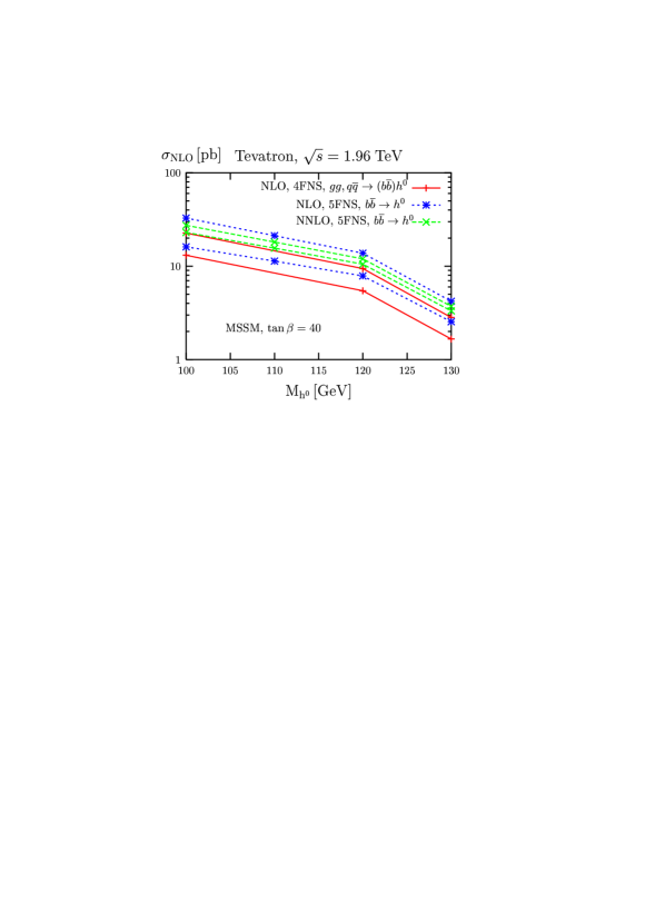
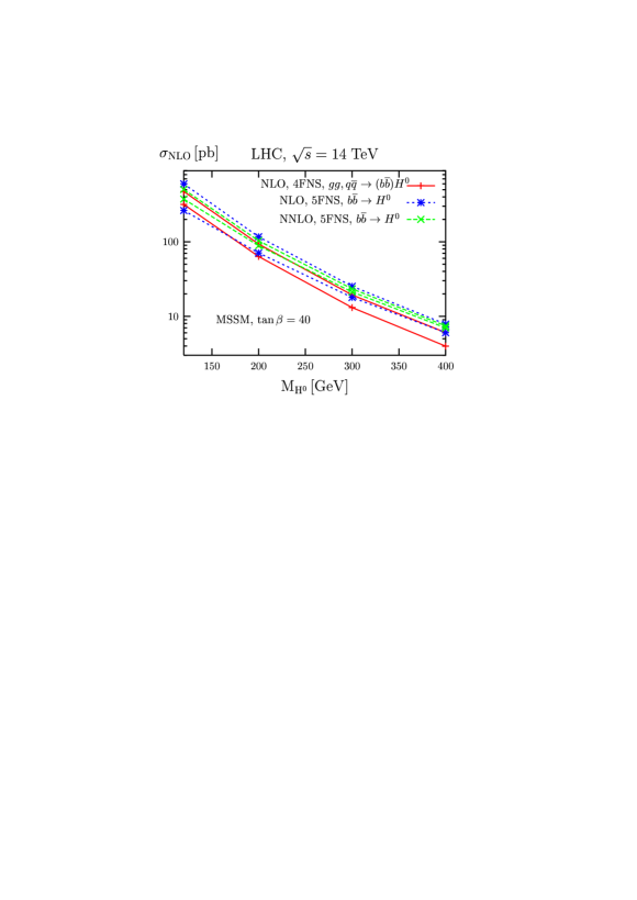
Figure 5: Total cross sections for $pp,p\bar{p}\rightarrow(b\bar{b})h$ ($h=h^{0},H^{0}$) in the MSSM with no bottom quark jet identified in the final state in the 4FNS (at NLO) and 5FNS (at NLO and NNLO) as a function of the light and heavy MSSM Higgs boson masses, at both the Tevatron and the LHC. The error bands have been obtained by varying the renormalization and factorization scales as described in the text.

IV.2 Results for semi-inclusive $b(\bar{b})h$ production

If a single bottom quark is tagged then the final state is $bh$ or $\bar{b}h$. A recent Tevatron study Avto:2005 used the search for neutral MSSM Higgs bosons in events with three bottom quarks in the final state ($bh+\bar{b}h$ production with $h\rightarrow b\bar{b}$) to impose limits on the $\tan\beta$ and $M_{A^{0}}$ parameter space. The effect of the NLO corrections in the 4FNS are illustrated in Fig. 6 where we show the SM results for the LO and NLO total production rates Dawson:2004tl . We see a strong reduction of the scale dependence at NLO. In Fig. 7 we compare the rates obtained in the MSSM for $\tan\beta=40$ for the single $b$-tagged events in the 4FNS and 5FNS schemes, where we varied separately the renormalization and factorization scales from $0.2\mu_{0}$ to $\mu_{0}$, with $\mu_{0}\!=\!m_{b}+M_{h}/2$. These are obtained by rescaling the SM results of Ref. Dawson:2004tl according to Eq. (7) to the MSSM scenario discussed in this review. Note that the resulting bands only give an estimate of the theoretical uncertainty due to residual scale dependence, but do not consider other uncertainties such as PDF uncertainties. A discussion of the PDF uncertainties can be found in Section V. As demonstrated in Fig. 7 the theoretical predictions in the 4FNS and 5FNS are fully compatible and, thus, either calculation can be used in the experimental analyses. The theoretical uncertainty in both schemes is still dominated by the residual scale dependence and the PDF uncertainty.

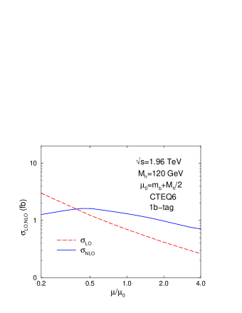
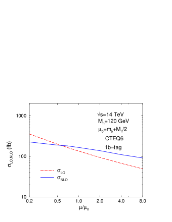
Figure 6: Total LO and NLO cross sections in the SM for $pp,p\bar{p}\rightarrow b(\bar{b})h$ production in the 4FNS as a function of $\mu\!=\!\mu_{r}\!=\!\mu_{f}$ for $M_{h}\!=\!120$ GeV, at both the Tevatron and the LHC.

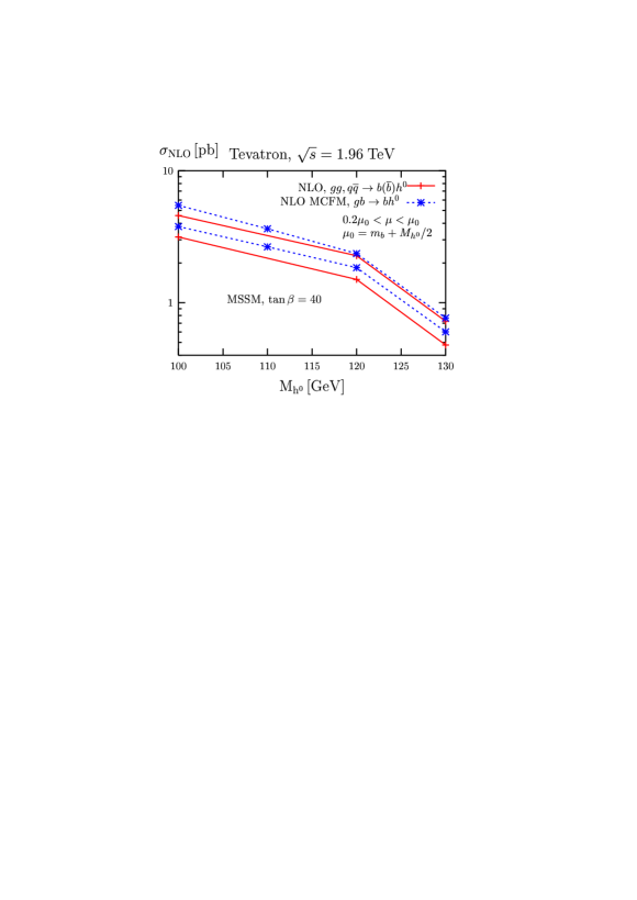
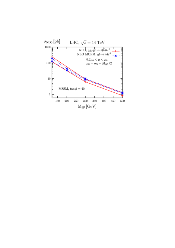
Figure 7: Total NLO cross section in the MSSM for $pp,p\bar{p}\rightarrow b(\bar{b})h$ production at the Tevatron and the LHC as a function of $M_{h^{0},H^{0}}$. We varied $\mu_{r}$ and $\mu_{f}$ independently to obtain the uncertainty bands, as explained in the text. The solid curves correspond to the 4FNS, the dashed curves to the 5FNS.

In comparing the four and five flavor number schemes it is particularly interesting to compare the kinematic distributions. In Figs. 8-9, we compare the results for the transverse momentum and pseudorapidity distributions of the light and heavy MSSM Higgs bosons, $h^{0}$ and $H^{0}$, in both the 4FNS and 5FNS, at the Tevatron and the LHC. We see, in general, good agreement between the two schemes within their respective theoretical uncertainties, except in regions of kinematic boundaries. This is particularly dramatic in the $p_{T}^{h}$ distributions in the 5FNS where, around $p_{T}^{h}\!\simeq\!20$ GeV, a kinematic threshold induced in $bg\rightarrow bh$ by the cut on the $p_{T}$ of the bottom quark causes the 5FNS NLO calculation to be unreliable. This instability can be reabsorbed by using a larger bin size (see inlays), and could therefore be interpreted as a sort of theoretical resolution for the 5FNS. The instabilities could be removed by a systematic resummation of threshold corrections Catani:1997xc ; DelDuca:2003uz , which is not implemented in MCFM.

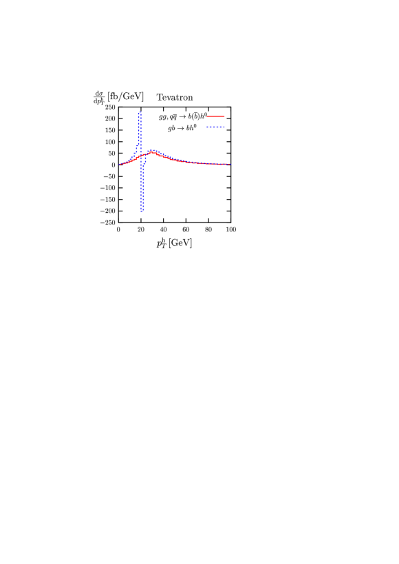
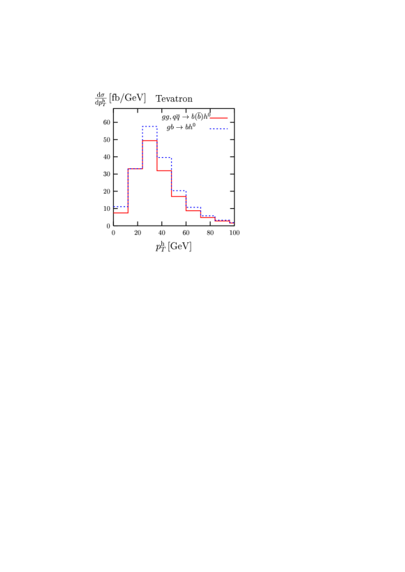
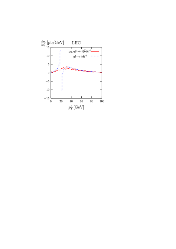
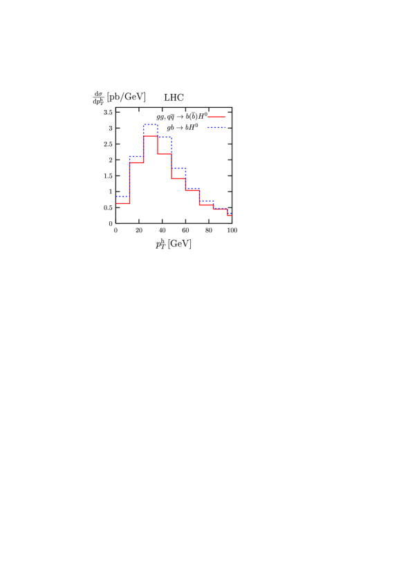
Figure 8: $d\sigma/dp_{T}^{h}$ in the MSSM at the Tevatron and the LHC for $M_{h^{0},H^{0}}\!=\!120$ GeV and $\mu_{r}\!=\!\mu_{F}\!=\!\mu_{0}/2$ for single $b$-tag events. We show the NLO results in the 4FNS (solid) and 5FNS (dashed), using two different bin sizes, 2 GeV (left) and 12 GeV (right).

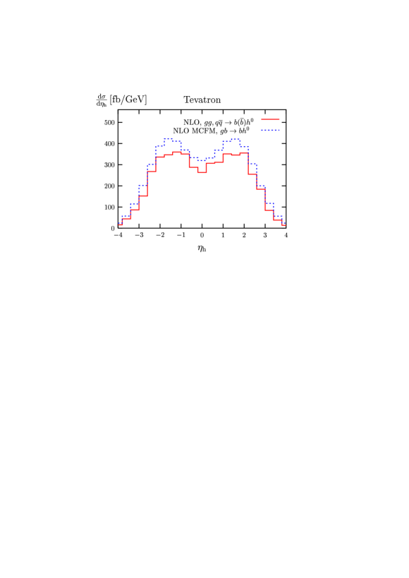
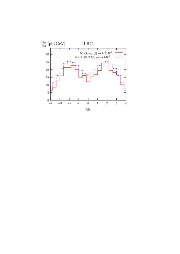
Figure 9: $d\sigma/d\eta_{h}$ in the MSSM at the Tevatron and the LHC for $M_{h^{0},H^{0}}\!=\!120$ GeV and $\mu_{r}\!=\!\mu_{f}\!=\!\mu_{0}/2$ for single $b$-tag events. We show the NLO results in the 4FNS (solid) and 5FNS (dashed).

IV.3 Results for exclusive $b\bar{b}h$ production

Finally, we discuss the fully exclusive LO and NLO cross sections for $b\bar{b}h$ production, where both the outgoing $b$ and $\bar{b}$ quarks are identified. The results of Ref. Dawson:2003ex that are presented here have been obtained by using the CTEQ5 set of PDFs. We have checked that the conclusions of the numerical discussion presented here do not change when using the CTEQ6 set of PDFs. In Fig. 10 we show, for $M_{h}\!=\!120$ GeV, the dependence of the LO and NLO total cross sections, calculated in the SM and in the 4FNS, on the arbitrary renormalization/factorization scale $\mu$ (with $\mu_{r}\!=\!\mu_{f}\!=\!\mu$). The curves labelled ”$OS$” (”$MS$”) use the on-shell (${\overline{MS}}$) scheme for the bottom Yukawa coupling. The NLO results have significantly less sensitivity to the scale choice, both in the $OS$ and in the $\overline{MS}$ schemes. However, while in the $OS$ scheme the plateau region, or region of least sensitivity to the renormalization/factorization scale, is around $\mu\!=\!\mu_{0}$, in the $\overline{MS}$ scheme it is shifted towards $\mu\!=\!\mu_{0}/2$, ($\mu_{0}\!=\!m_{b}+M_{h}/2$). It is interesting to note, that the scale choice $\mu=M_{h}/4$ is supported by theoretical studies Harlander:2003ai and corresponds to the point where the NNLO rate for inclusive Higgs production from bottom quarks is the same as the NLO rate Boos:2003yi ; Maltoni:2003pn . Fig. 10 shows how the $\overline{MS}$ scheme gives a perturbative cross section that is better behaved over a broader range of scales, and therefore preferable. Conservatively, one could interpret the difference between the two plateau regions as an additional 10-20% theoretical error.

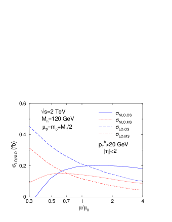
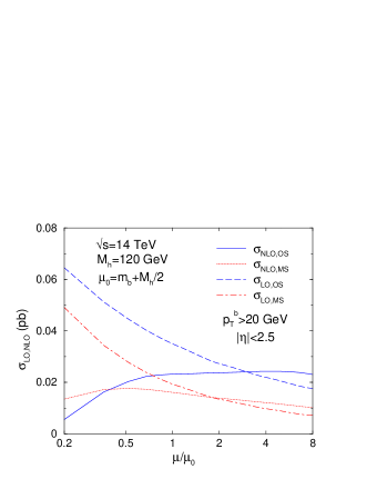
Figure 10: Total LO and NLO cross sections in the SM for the two $b$-tag process, $pp,p\bar{p}\rightarrow b\bar{b}h$, in the 4FNS as a function of $\mu\!=\!\mu_{r}\!=\!\mu_{f}$ for $M_{h}\!=\!120$ GeV, at both the Tevatron and the LHC. Results are shown for both the $\overline{MS}$ and $OS$ renormalization scheme for the bottom Yukawa coupling (see discussion in Section II.3).

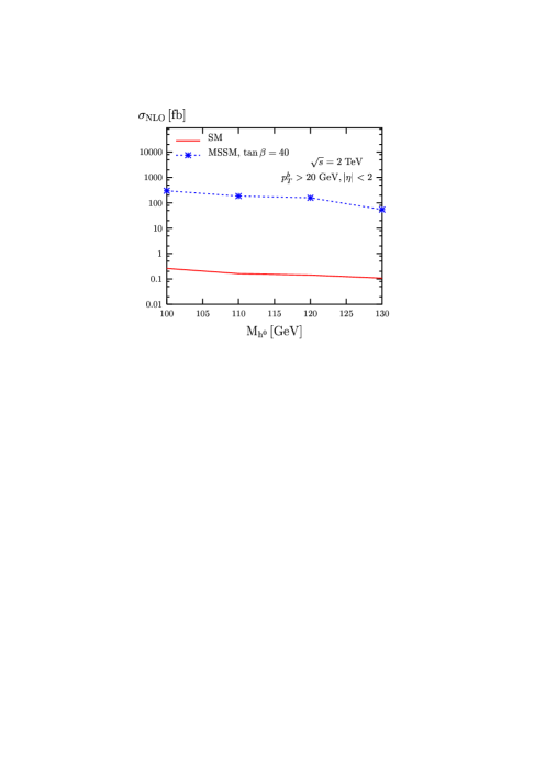
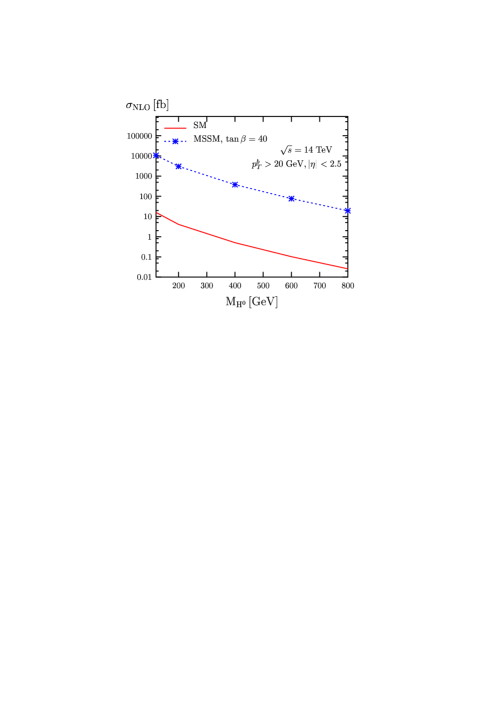
Figure 11: Total NLO cross sections in the SM and MSSM for the two $b$-tag process, $pp,p\bar{p}\rightarrow b\bar{b}h$, in the 4FNS for the central scale $\mu_{r}\!=\!\mu_{f}\!=\!\mu_{0}$. Shown is the dependence on the light and heavy MSSM Higgs boson masses at the Tevatron and the LHC, respectively.

In Fig. 11 we compare the production of the SM Higgs boson with that of the neutral scalar Higgs bosons of the MSSM and again observe a significant enhancement of the rate in the MSSM for large $\tan\beta$. The MSSM results have been obtained from the SM results as described in Eq. 7 by using the rescaling factors of Tables 1, 2 for $\tan\beta=40$.

Finally, in Figs. 12, 13 we illustrate the impact of NLO QCD corrections on the transverse momentum and pseudorapidity distribution of the SM Higgs boson and the bottom quark by showing the relative correction, $d\sigma_{NLO}/d\sigma_{LO}-1$ (in percent). For the renormalization/factorization scale we choose $\mu=2\mu_{0}$ at the Tevatron and $\mu=4\mu_{0}$ at the LHC. These two scale choices are well within the plateau regions where the NLO cross sections vary the least with the value of $\mu$. As can be seen, the NLO QCD corrections can considerably affect the shape of kinematic distributions, and their effect cannot be obtained from simply rescaling the LO distributions with a K-factor of $\sigma_{\scriptscriptstyle NLO}/\sigma_{\scriptscriptstyle LO}\!=\!1.38\pm 0.02$ (Tevatron, $\mu\!=\!2\mu_{0}$) and $\sigma_{\scriptscriptstyle NLO}/\sigma_{\scriptscriptstyle LO}\!=\!1.11\pm 0.03$ (LHC, $\mu\!=\!4\mu_{0}$). The errors only include the statistical uncertainty from the Monte Carlo integration. The kinematic distributions have been calculated within the SM and using the $OS$ scheme, but we see a similar behavior when using the $\overline{MS}$ bottom quark Yukawa coupling or consider the MSSM case.

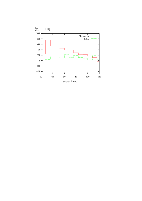
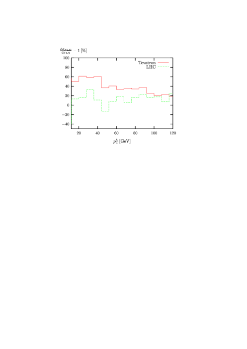
Figure 12: The relative corrections $d\sigma_{\scriptscriptstyle NLO}/d\sigma_{\scriptscriptstyle LO}-1$ for the $p_{T}$ distribution of the bottom or anti-bottom quark with the largest $p_{T}$ ($p_{T,max}$) (left) and of the SM Higgs boson ($p_{T}^{h}$) (right) to $b\bar{b}h$ production in the SM at the Tevatron (with $\sqrt{s}\!=\!2$ TeV and $\mu\!=\!2\mu_{0}$) and the LHC (with $\sqrt{s}\!=\!14$ TeV and $\mu\!=\!4\mu_{0}$).

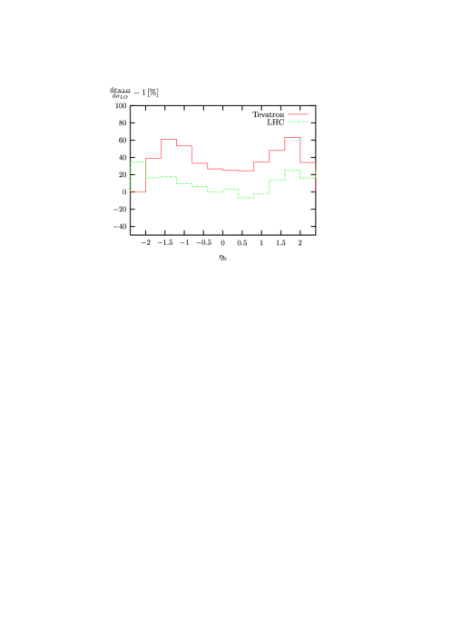
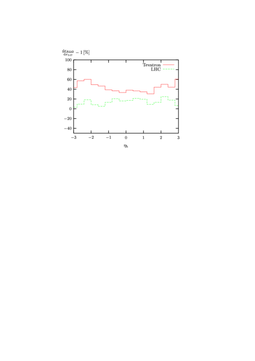
Figure 13: The relative corrections $d\sigma_{\scriptscriptstyle NLO}/d\sigma_{\scriptscriptstyle LO}-1$ for the $\eta$ distribution of the bottom quark $\eta_{b}$ (left) and of the SM Higgs boson ($\eta_{h}$) (right) to $b\bar{b}h$ production in the SM at the Tevatron (with $\sqrt{s}\!=\!2$ TeV and $\mu\!=\!2\mu_{0}$) and the LHC (with $\sqrt{s}\!=\!14$ TeV and $\mu\!=\!4\mu_{0}$).

V PDF Uncertainties

Besides the residual renormalization/factorization scale dependence after the NLO corrections have been included, another major source of theoretical uncertainty for cross section predictions at hadron colliders comes from the Parton Distribution Functions. Unfortunately, PDFs are plagued by uncertainties either from the non-perturbative starting distributions used to fit the data or from the perturbative DGLAP evolution to the higher energies relevant at hadron colliders Gribov:1972 ; Altarelli:1977zs ; Dokshitzer:1977 .

Recently, several collaborations have introduced new schemes which allow an estimate of theoretical uncertainties on physical observables due to the uncertainty in the PDFs. Here, we focus on the scheme introduced by the CTEQ collaboration based on the Hessian matrix method CTEQ:2002 and study the uncertainties of semi-inclusive total $b\bar{b}h$ production rates that are induced by the uncertainties in the PDFs. The details of this method are beyond the scope of this review, however, we give a brief explanation below. First, the nominal set of PDFs (e.g. CTEQ6) is constructed by fitting a non-perturbative core equation to data from low-energy experiments designed to measure PDFs. The core equation, in the method used by CTEQ, is parameterized by 20 independent parameters which are dialed to fit the data. Once the nominal set is fixed, the 20 parameters are then varied in a well-defined manner to produce an additional 40 sets of PDFs. These sets serve as a map of the neighborhood around the nominal fit to the data. Indeed, one can then use the 40 sets to estimate the uncertainty from the PDFs on a physical observable in the following way Ferrag:2003 : first, the central value cross section $\sigma_{0}$ is calculated using the global minimum PDF (i.e. CTEQ6M). The calculation of the cross section is then performed with the additional 40 sets of PDFs to produce 40 different predictions, $\sigma_{i}$. For each of these, the deviation from the central value is calculated to be $\Delta\sigma_{i}^{\pm}=|\sigma_{i}-\sigma_{0}|$ when ${\sigma_{i}}_{<}^{>}\sigma_{0}$. Finally, to obtain the uncertainties due to the PDFs the deviations are summed quadratically as $\Delta\sigma^{\pm}=\sqrt{\sum_{i}{\Delta\sigma^{\pm}_{i}}^{2}}$ and the cross section including the theoretical uncertainties arising from the PDFs is quoted as $\sigma_{0}|^{+\Delta\sigma^{+}}_{-\Delta\sigma^{-}}$. Recently, similar analyses have been performed for the dominant SM Higgs production modes Djouadi:2003pd and for the fully inclusive Higgs production modes in both the SM ($gg\to h$) and the MSSM ($b\bar{b}\to h$) Belyaev:2005nu .

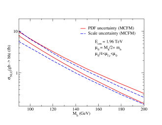
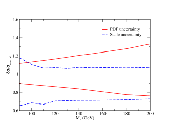
Figure 14: Comparison between theoretical uncertainties due to scale dependence and uncertainties arising from the PDFs at the Tevatron. In the bottom plot, both uncertainty bands have been normalized to the central value of the total cross section $\sigma_{0}$.

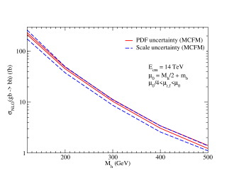
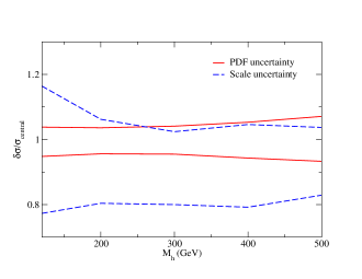
Figure 15: Comparison between theoretical uncertainties due to scale dependence and uncertainties arising from the PDFs at the LHC. In the bottom plot, both uncertainty bands have been normalized to the central value of the total cross section $\sigma_{0}$.

In Figs. 14 and 15 we plot the total SM NLO cross section for $bg\rightarrow bh$ obtained with MCFM MCFM:2004 at the Tevatron and LHC respectively. Here, we compare the spread uncertainties from residual scale dependence and the PDFs both for the total cross section (top) and the total cross section normalized to the central value calculated with CTEQ6M (bottom).

From Fig. 15 one can see that, at the LHC, the theoretical uncertainty is dominated by the residual scale dependence. Due to the large center of mass (c.o.m.) energy of the LHC, the gluons and bottom quarks in the initial state have small momentum fraction ($x$) values and, hence, small PDF uncertainties typically in the 5-10% range.

In contrast, due to the smaller c.o.m. energy, the PDF uncertainties at the Tevatron (Fig. 14) are comparable and even larger than the uncertainties due to residual scale dependence over the full Higgs mass range. The smaller c.o.m. energy results in higher-$x$ gluons and bottom quarks in the initial state which corresponds to large PDF uncertainties in the 10-30% range.

Finally, in Fig. 16, we plot the normalized total SM NLO cross sections of $bg\rightarrow bh$ and $gg\rightarrow b(\bar{b})h$ and compare their respective uncertainties due to the PDFs. We see that, at both the Tevatron and the LHC, the PDF uncertainties are almost identical for both the $gg$ and $bg$ initial states.

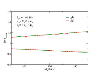
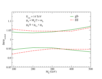
Figure 16: Normalized cross sections for Higgs production with one $b$ jet at the Tevatron (top) and the LHC (bottom) showing the uncertainty from PDFs for both the $gg$ and $bg$ initial states.

VI Conclusions

We discussed the status of theoretical predictions for Higgs boson production in association with bottom quarks for the cases where zero, one or both outgoing bottom quarks are identified. These processes are important Higgs boson discovery modes in models with enhanced bottom quark Yukawa couplings, such as the MSSM at large values of $\tan\beta$. We presented results for the MSSM $b\bar{b}h$ ($h=h^{0},H^{0}$) total and differential production rates at $\tan\beta=40$ and discussed the theoretical uncertainties of the state-of-the-art predictions due to the residual renormalization/factorization scale dependence at NLO (NNLO) in QCD and the uncertainty in the PDFs. We have shown that the total cross section for the inclusive case, $pp,p\bar{p}\rightarrow(b\bar{b})h$, and both the total and differential cross sections for the semi-inclusive case, $pp,p\bar{p}\rightarrow b(\bar{b})h$, within a 4FNS and 5FNS are fully compatible within the existing theoretical errors. All important Higgs production processes at hadron colliders are now known at NLO, and some even at NNLO, and the theoretical uncertainties of the QCD predictions are well under control.

References

- (1) The ALEPH, DELPHI, L3, OPAL Collaborations, and the LEP Higgs Working Group, Phys. Lett. B565, 61 (2003).
- (2) The LEP Higgs Working Group, LHWG-Note 2004-01 (August 2004).
- (3) The LEP Electroweak Working Group, hep-ex/0412015, update Summer 2005 at webpage: lepewwg.web.cern.ch/LEPEWWG/stanmod/summer2005results.
- (4) M. Carena and H.E. Haber, Prog. Part. Nucl. Phys. 50, 63 (2003).
- (5) T. Han and S. Willenbrock, Phys. Lett. B273, 167 (1991).
- (6) T. Han, G. Valencia, and S. Willenbrock, Phys. Rev. Lett. 69, 3274 (1992).
- (7) S. Dawson, Nucl. Phys. B359, 283 (1991).
- (8) A. Djouadi, M. Spira, and P.M. Zerwas, Phys. Lett. B264, 440 (1991).
- (9) D. Graudenz, M. Spira, and P.M. Zerwas, Phys. Rev. Lett. 70, 1372 (1993).
- (10) M. Spira, A. Djouadi, D. Graudenz, D. and P.M. Zerwas, Phys. Lett. B264, 440 (1991).
- (11) W. Beenakker, S. Dittmaier, M. Krämer, B. Plümper, M. Spira, and P.M. Zerwas, Phys. Rev. Lett. 87, 201805 (2001).
- (12) L. Reina and S. Dawson, Phys. Rev. Lett. 87, 201804 (2001).
- (13) L. Reina, S. Dawson, and D. Wackeroth, Phys. Rev. D65, 053017 (2002).
- (14) W. Beenakker, S. Dittmaier, M. Krämer, B. Plümper, M. Spira, and P.M. Zerwas, Nucl. Phys. B653, 151 (2003).
- (15) S. Dawson, L.H. Orr, L. Reina, and D. Wackeroth, Phys. Rev. D67, 071503 (2003).
- (16) S. Dawson, C. Jackson, L.H. Orr, L. Reina, and D. Wackeroth, Phys. Rev. D68, 034022 (2003).
- (17) R.V. Harlander and W.B. Kilgore, Phys. Rev. Lett. 88, 201801 (2002).
- (18) C. Anastasiou and K. Melnikov, Nucl. Phys. B646, 220 (2002).
- (19) R.V. Harlander and W.B. Kilgore, Phys. Rev. D68, 013001 (2003).
- (20) S. Catani, D. de Florian, and M. Grazzini, JHEP 05, 025 (2001).
- (21) V. Ravindran, J. Smith, and W.L. Van Neerven, Nucl. Phys. B634, 247 (2002).
- (22) O. Brein, A. Djouadi, and R. Harlander, Phys. Lett. B579, 149 (2004).
- (23) J. Campbell et al., in 3rd Les Houches Workshop Physics at TeV Colliders, 2003, hep-ph/0405302.
- (24) The D0 Collaboration, hep-ex/0504018.
- (25) The CDF Collaboration, “Search for Neutral MSSM Higgs Bosons Decaying to Tau Pairs”, CDF 7676 (2005).
- (26) S. Dittmaier, M. Krämer, and M. Spira, Phys. Rev. D70, 074010 (2004).
- (27) S. Dawson, C. Jackson, L. Reina, and D. Wackeroth, Phys. Rev. Lett. 94, 031802 (2005).
- (28) J. Campbell, R.K. Ellis, F. Maltoni, and S. Willenbrock, Phys. Rev. D67, 095002 (2003).
- (29) S. Dawson, C. Jackson, L. Reina, and D. Wackeroth, Phys. Rev. D69, 074027 (2004).
- (30) S. Heinemeyer, Eur. Phys. J. C22, 521 (2001).
- (31) M. Frank, S. Heinemeyer, W. Hollik, and G. Weiglein, hep-ph/0212037.
- (32) S. Heinemeyer, hep-ph/0407244.
- (33) J. Pumplin, D.R. Stump, J. Huston, H.L. Lai, P. Nadolsky, and W.-K. Tung, JHEP 0207, 012 (2002).
- (34) R. Barnett, H. Haber, D. Soper, Nucl. Phys. B306, 697 (1988).
- (35) F. Olness, W.-K. Tung, Nucl. Phys. B308, 813 (1988).
- (36) D. Dicus, T. Stelzer, Z. Sullivan, S. Willenbrock, Phys. Rev. D39, 751 (1989).
- (37) V. Gribov and L. Lipatov, Sov. J. Nucl. 15, 438 (1972).
- (38) G. Altarelli and G. Parisi, Nucl. Phys. B126, 298 (1977).
- (39) Y. Dokshitzer, Sov. J. Nucl. 46, 641 (1977).
- (40) D. Dicus, T. Stelzer, Z. Sullivan, S. Willenbrock, Phys. Rev. D59, 094016 (1999).
- (41) J. Campbell and R.K. Ellis, webpage: mcfm.fnal.gov.
- (42) J.F. Gunion, H. E. Haber, G. L. Kane, and S. Dawson, The Higgs Hunter’s Guide (Addison-Wesley, Menlo Park) 1990.
- (43) T. Hahn, S. Heinemeyer, W. Hollik, and G. Weiglein, webpage: www.feynhiggs.de (Version 2.2.10).
- (44) M. Carena, D. Garcia, U. Nierste, and C. E. M. Wagner, Nucl. Phys. B577, 88 (2000).
- (45) A. Djouadi, J. Kalinowski, and M. Spira, Comput. Phys. Commun. 108, 56 (1998).
- (46) J.S. Lee et al., Comput. Phys. Commun. 156, 283 (2004).
- (47) J.S. Lee et al., webpage: theory.ph.man.ac.uk/jslee/CPsuperH.html.
- (48) H.L. Lai et al., The CTEQ Collaboration, Eur. Phys. J. C12, 375 (2000).
- (49) S. Catani and B.R. Webber, JHEP 10, 005 (1997).
- (50) V. Del Duca, F. Maltoni, Z. Nagy, and Z. Trocsanyi, JHEP 04, 059 (2003).
- (51) E. Boos and T. Plehn, Phys. Rev. D69, 094005 (2004).
- (52) F. Maltoni, Z. Sullivan, and S. Willenbrock, Phys. Rev. D67, 093005 (2003).
- (53) S. Ferrag and B. Lagorge, ATLAS-COM-2003-13.
- (54) A.D. Martin, R.G. Roberts, W.J. Stirling, and R.S. Thorne, Eur. Phys. J. C28, 455 (2003).
- (55) A. Djouadi and S. Ferrag, Phys. Lett. B586, 345 (2003).
- (56) A. Belyaev, J. Pumplin, W.K. Tung and C.P. Yuan, hep-ph/0508222.