Forty-fifth anniversary
of the Nambu–Jona-Lasinio model

Abstract

A short review of the development of the Nambu–Jona-Lasinio (NJL) model is given. The $SU(2)\times SU(2)$ and $U(3)\times U(3)$ local quark NJL models are considered. The mechanisms of spontaneous breaking of chiral symmetry and vector dominance are shown. The local NJL model allows us to describe the mass spectrum and main strong and electroweak decays of the four ground-state nonets of pseudoscalar, scalar, vector and axial-vector mesons. Applications of this model to the description of mesons in hot and dense medium are discussed. It is shown that for solving problems connected with the description of the meson radial excitations and quark confinement it is necessary to consider a nonlocal extension of the NJL model. The main attention is attracted to the description of the methods used in different versions of the NJL model. Physical results for low-energy hadron physics obtained in these models can be found in the cited works.

Bogoliubov Laboratory of Theoretical Physics,
Joint Institute for Nuclear Research, 141980 Dubna, Russia

1 Introduction

The NJL model was proposed in 1961, where the authors attempted to explain the origin of the nucleon mass with the help of spontaneous breaking of chiral symmetry [1]. The model was formulated in terms of nucleons, pions and scalar $\sigma$ mesons. Remind that the fundamental theory of strong interactions, QCD, was not constructed at that time.

After 15 years this model was reformulated at the quark language by the Japanese physicists T. Eguchi and K. Kikkawa [4, 5]. It should be noted that it is supposed that all hadrons are formed from constituent quarks with mass $m\approx 300$ MeV, whereas the QCD theory is based on more light current quarks with mass $m_{0}\approx 5-7$ MeV. In [4, 5], it is shown that light current quarks turn into the massive constituent quarks due to spontaneous breaking of chiral symmetry. However, they only considered the quark NJL model in the chiral limit $m_{0}=0$. In this limit all masses of pseudoscalar mesons are equal to zero.

Starting from 1982 M.K. Volkov and D. Ebert with collaborators considered a more realistic version of the quark NJL model when $m_{0}\neq 0$ [6, 7, 8]. It allowed them to describe the mass spectrum, internal properties, and strong and electroweak interactions of scalar, pseudoscalar, and vector meson nonets [9, 10]. In 1984, T. Hatsuda and T. Kunihiro applied this model to the description of hadrons in hot dense medium [11, 12].

After 1986 this model gained popularity. In the following years more than six hundred papers devoted to the NJL model were published. Therefore, we cannot give here a full list of the corresponding references. We only note some authors who gave a noticeable contribution in this field of research.

The NJL model was especially intensively used for different applications in Germany (D. Ebert, Humboldt Univ., Berlin; H. Kleinert, Freie Univ., Berlin; H. Reinhardt, Tubingen Univ.; J. Hufner, S. Klevansky, Heidelberg Univ.; W. Weise Munich, Tech. Univ.; D. Blaschke, G. Roepke Rostock Univ.; K. Goeke, C.V. Christov Ruhr Univ., Bochum; B. Friman Darmstadt GSI and others), Japan (T. Hatsuda, K. Yazaki Tokyo Univ.; T. Kunihiro Kyoto Univ.; M. Asakawa, S. Sawada, K. Yamawaki Nagoya Univ. and others) and USA (M.D. Scadron Arizona Univ.; C.M. Shakin City Coll., N.Y. and others). The NJL model was also studied by many physicists from China, England, France, Italy, Portugal, South African Republic and other countries.

In our country this model was actively developed at JINR Dubna (M.K. Volkov, G.V. Efimov, M.I. Ivanov, Yu.L. Kalinovsky, A.A. Osipov with collaborators), St.-Petersburg State Univ. (A.A. Andrianov and V.A. Andrianov), St.-Petersburg INP (D. Diakonov, V.Yu. Petrov) and St.-Petersburg Polytechnic Inst. (A.N. Ivanov).

It is worthwhile to note that now NJL is widely used for different applications as in elementary particle physics as in nuclear physics (see e.g. [13, 14]).

2 $SU(2)\times SU(2)$ NJL model

2.1 Pseudoscalar and scalar mesons

Firstly, let us consider the simple $SU(2)\times SU(2)$ NJL model. The corresponding chiral quark Lagrangian is

$$\mathcal{L}(\bar{q},q)=\bar{q}(x)(i\hat{\partial}_{x}-m_{0})q(x)+\frac{G_{\pi}}{2}\left((\bar{q}(x)q(x))^{2}+(\bar{q}(x)i\tau_{a}\gamma^{5}q(x))^{2}\right),$$ (1)

where $\bar{q}(x)=\{u(x),d(x)\}$ are the fields of $u$, $d$ antiquarks, $m_{0}$ is the current quark mass, $G_{\pi}$ is the four-quark coupling constant, $\tau^{a}$ are the Pauli matrices, and $\gamma^{5}$ is the Dirac matrix.

After bosonization the Lagrangian takes the form

$$\mathcal{L}(\bar{q},q,\sigma,\pi)=\bar{q}(x)(i\hat{\partial}_{x}-m_{0}+\sigma(x)+i\gamma_{5}\tau_{a}\pi_{a}(x))q(x)-\frac{\sigma^{2}(x)+\pi_{a}^{2}(x)}{2G_{\pi}},$$ (2)

where $\sigma(x)$, $\pi_{a}(x)$ are the scalar and pseudoscalar meson fields. Effective meson Lagrangian can be obtained from Lagrangian (2) in one quark-loop approximation. Here we can see that vacuum expectation value of pion field is equal to zero, whereas $\sigma(x)$ has a nonzero vacuum expectation value $\langle\sigma\rangle_{0}=\sigma_{0}$. Therefore, it is necessary to redefine this field in order a new physical field $\sigma^{\prime}(x)=\sigma(x)-\sigma_{0}$ have a zero vacuum expectation value $\langle\sigma^{\prime}\rangle_{0}=0$. Excluding linear in $\sigma^{\prime}(x)$ terms from the Lagrangian we obtain gap equation

$$\left.\frac{\delta\mathcal{L}}{\delta\sigma^{\prime}}\right|_{\sigma^{\prime}=0}=0,\quad\Rightarrow\quad m_{0}=m+\sigma_{0}=m(1-8G_{\pi}I_{1}^{\Lambda}(m))$$ (3)

This equation describes spontaneous breaking of chiral symmetry. As a result, light current quark mass $m_{0}$ turns into massive constituent quark mass $m$. Note that all physical quantities in the NJL model are expressed through the quadratically and logarithmically divergent integrals $I_{1}^{\Lambda}(m)$ and $I_{2}^{\Lambda}(m)$

$$I_{1}^{\Lambda}(m) = \frac{N_{c}}{(2\pi)^{4}}\int\frac{d_{E}^{4}k\Theta(\Lambda^{2}-k^{2})}{m^{2}+k^{2}}=\frac{N_{c}}{4\pi^{2}}\left[\Lambda^{2}-m^{2}\ln\left(\frac{\Lambda^{2}}{m^{2}}+1\right)\right]$$ (4)

$$I_{2}^{\Lambda}(m) = \frac{N_{c}}{(2\pi)^{4}}\int\frac{d_{E}^{4}k\Theta(\Lambda^{2}-k^{2})}{(m^{2}+k^{2})^{2}}=\frac{N_{c}}{4\pi^{2}}\left[\ln\left(\frac{\Lambda^{2}}{m^{2}}+1\right)-\left(1+\frac{m^{2}}{\Lambda^{2}}\right)^{-1}\right]$$

These integrals are given in Euclidean space; $N_{c}=3$ is a number of quark colors; $\Lambda$ is the cut-off parameter. It describes the region where spontaneous breaking of chiral symmetry takes place.

From the Lagrangian (2) the following expressions for the $\pi$ and $\sigma$ meson masses can be obtained

$$m_{\pi}^{2}=g_{\pi qq}^{2}\left(\frac{1}{G_{\pi}}-8I_{1}^{\Lambda}(m)\right),\quad m_{\sigma}^{2}=m_{\pi}^{2}+4m^{2},$$ (5)

where $g_{\pi qq}=g_{\sigma qq}=(4I_{2}^{\Lambda}(m))^{-1/2}$ are the meson renormalization constants that provide a correct coefficient in the kinetic terms for the meson Lagrangian. It is easy to see from eqs. (3) and (5) that the pion mass is proportional to the first power of current quark mass (Gell-Mann–Oakes–Renner relation). As a result the pion become the Goldstone particle with zero mass in the chiral limit $m_{0}=0$.

From the weak pion decay $\pi\to\mu\nu$ the Goldberger-Treiman relation follows:

$$F_{\pi}=\frac{m}{g_{\pi qq}},$$ (6)

where $F_{\pi}=93$ MeV is the weak pion decay constant [15].

2.2 Vector and axial-vector mesons

The quark Lagrangian corresponding to the vector and axial-vector mesons is

$$\mathcal{L}(\bar{q},q)=-\frac{G_{\rho}}{2}\left((\bar{q}(x)\gamma^{\mu}\tau_{a}q(x))^{2}+(\bar{q}(x)\gamma^{\mu}\gamma^{5}\tau_{a}q(x))^{2}\right).$$ (7)

After bosonization this Lagrangian takes the form

$$\mathcal{L}(\bar{q},q,\rho,a_{1})=\bar{q}(x)(\gamma^{\mu}\tau_{a}\rho^{\mu}_{a}(x)+\gamma^{\mu}\gamma^{5}\tau_{a}{a_{1}}^{\mu}_{a})q(x)+\frac{({\rho}^{\mu}_{a})^{2}+({a_{1}}^{\mu}_{a})^{2}}{2G_{\rho}},$$ (8)

where $\rho^{\mu}_{a}$, ${a_{1}}^{\mu}_{a}$ are the fields of vector ($\rho$) and axial-vector ($a_{1}$) mesons.

Note that in the description of vector and axial-vector mesons a gauge-invariant regularization must be used [9]. The quark loop with two vector vertices defines the kinetic term of the vector meson and renormalization constant of the vector field $g_{\rho qq}$. As a result, the simple relation between $g_{\sigma qq}$ and $g_{\rho qq}$ appears [5, 9]

$$g_{\rho qq}=\sqrt{6}g_{\sigma qq}$$ (9)

We obtain for the $\rho$-meson mass

$$M_{\rho}^{2}=\frac{g_{\rho qq}^{2}}{4G_{\rho}}.$$ (10)

The renormalization constant of the $a_{1}$ meson field $g_{a_{1}qq}$ coincides with $g_{\rho qq}$ and the mass equals

$$M_{a_{1}}^{2}=M_{\rho}^{2}+6m^{2}$$ (11)

2.3 $\pi-a_{1}$ transitions

In the NJL model there are quark loops with pseudoscalar and axial-vector vertices that describe $\pi-a_{1}$ transitions [9, 16, 17, 18].

These transitions lead to nondiagonal terms in meson Lagrangian of the type $\sqrt{6}m{a_{1}}^{\mu}_{a}(x)\partial^{\mu}_{x}\pi_{a}(x)$. In order to exclude these terms it is necessary to redefine the axial-vector field as

$${a_{1}}^{\mu}_{a}(x)={a_{1}^{\prime}}^{\mu}_{a}(x)-\frac{\sqrt{6}m}{M_{a_{1}}^{2}}\partial^{\mu}_{x}\pi_{a}(x)$$ (12)

This leads to additional kinetic terms of the pions and to modification of the renormalization constant $g_{\pi qq}$. Now this constant is not equal to $g_{\sigma qq}$

$$g_{\pi qq}=Z^{1/2}g_{\sigma qq},\quad Z=\left(1-\frac{6m^{2}}{M_{a_{1}}^{2}}\right)^{-1}$$ (13)

It is interesting to note that allowance for the $\pi-a_{1}$ transitions does not affect to Goldberger-Treiman relation.

2.4 Numerical estimations

Let us define the model parameters. From eqs. (6), (9), (13) we can define constituent quark mass thought the observables $F_{\pi}=93$ MeV, $g_{\rho qq}=6.14$ (this value corresponds to the experimental width of $\rho$ meson) and $M_{a_{1}}=1.26$ GeV [15]

$$g_{\rho qq}=\sqrt{6}g_{\sigma qq}=\sqrt{\frac{6}{Z}}g_{\pi qq}=\sqrt{\frac{6}{Z}}\frac{m}{F_{\pi}}=\sqrt{6\left(1-\frac{6m^{2}}{M_{a_{1}}^{2}}\right)}\frac{m}{F_{\pi}}.$$ (14)

Then

$$m^{2}=\frac{M_{a_{1}}^{2}}{12}\left(1-\sqrt{1-\frac{4g_{\rho qq}^{2}F_{\pi}^{2}}{M_{a_{1}}^{2}}}\right)\quad\Rightarrow\quad m=280\,\mathrm{MeV}$$ (15)

The parameter $\Lambda$ can be found from the equation

$$g_{\rho qq}=\sqrt{\frac{6}{4I_{2}}}\quad\Rightarrow\quad\Lambda=1.25\,\mathrm{GeV}$$ (16)

$G_{\pi}$ and $G_{\rho}$ can be found from equations (5), (10) for pion and $\rho$-meson masses. Therefore, $G_{\pi}=4.9$ GeV^-2 and $G_{\rho}=16$ GeV^-2. The value of the current quark mass $m_{0}$ is defined from the gap equation (3), $m_{0}=3$ MeV.

3 $U(3)\times U(3)$ NJL model

In order to introduce strange mesons in the model, it is necessary to replace the Pauli matrices $\tau_{i}$ (i=1..3) by the Gell-Mann matrices $\lambda_{i}$ (i=0..8, where $\lambda_{0}=\sqrt{\frac{2}{3}}\mathbf{1}$). Let us remind that the $U_{A}(1)$ problem exists connected with a correct description of masses of $\eta$, $\eta^{\prime}$ mesons. Indeed, by using the $U(3)\times U(3)$ symmetric Lagrangian we obtain ”ideal” singlet-octet mixing for pseudoscalar isoscalar mesons. Then, one of these states contains only $u$ and $d$ quarks and the other state contains only the strange quark. This situation contradicts experimental data.

In order to solve this problem it is necessary to add the t‘Hooft interaction [19] to NJL Lagrangian [20, 21, 22, 23]. As a result the model for scalar and pseudoscalar meson nonets consist of two Lagrangians

$$\mathcal{L}^{NJL} = {\bar{q}}(i{\hat{\partial}}-m^{0})q+{G\over 2}\sum_{i=0}^{8}[({\bar{q}}{\lambda}_{i}q)^{2}+({\bar{q}}i{\gamma}_{5}{\lambda}_{i}q)^{2}],$$

$$\mathcal{L}^{tH} = -K\left({\det}[{\bar{q}}(1+\gamma_{5})q]+{\det}[{\bar{q}}(1-\gamma_{5})q]\right),$$ (17)

where $\bar{q}=\{\bar{u},\bar{d},\bar{s}\}$ are antiquark fields, $m^{0}$ is a current quark mass matrix with diagonal elements $m^{0}_{u}$, $m^{0}_{d}$, $m^{0}_{s}$ $(m^{0}_{u}\approx m^{0}_{d})$.

The Lagrangian (17) can be rewritten in the form (see [21])

$$\mathcal{L}={\bar{q}}(i{\hat{\partial}}-m^{0})q+{\frac{1}{2}}\sum_{i=1}^{9}[G_{i}^{(-)}({\bar{q}}{\lambda^{\prime}}_{i}q)^{2}+G_{i}^{(+)}({\bar{q}}i{\gamma}_{5}{\lambda^{\prime}}_{i}q)^{2}]+$$

$$\qquad+G^{(-)}_{us}({\bar{q}}{\lambda}_{u}q)({\bar{q}}{\lambda}_{s}q)+G_{us}^{(+)}({\bar{q}}i{\gamma}_{5}{\lambda}_{u}q)({\bar{q}}i{\gamma}_{5}{\lambda}_{s}q)~{},$$ (18)

where

$${\lambda^{\prime}}_{i}={\lambda}_{i}~{}~{}~{}(i=1,...,7),~{}~{}~{}\lambda^{\prime}_{8}=\lambda_{u}=({\sqrt{2}}\lambda_{0}+\lambda_{8})/{\sqrt{3}},$$

$$\lambda^{\prime}_{9}=\lambda_{s}=(-\lambda_{0}+{\sqrt{2}}\lambda_{8})/{\sqrt{3}},$$

$$G_{1}^{(\pm)}=G_{2}^{(\pm)}=G_{3}^{(\pm)}=G\pm 4Km_{s}I_{1}^{\Lambda}(m_{s}),$$

$$G_{4}^{(\pm)}=G_{5}^{(\pm)}=G_{6}^{(\pm)}=G_{7}^{(\pm)}=G\pm 4Km_{u}I_{1}^{\Lambda}(m_{u}),$$

$$G_{u}^{(\pm)}=G\mp 4Km_{s}I_{1}(m_{s}),~{}~{}~{}G_{s}^{(\pm)}=G,~{}~{}~{}G_{us}^{(\pm)}=\pm 4{\sqrt{2}}Km_{u}I_{1}^{\Lambda}(m_{u}).$$ (19)

The t‘Hooft interaction leads to the additional terms in the gap equations for the $u$, $s$ quark masses

$$m_{u} = m_{u}^{0}+8m_{u}GI_{1}^{\Lambda}(m_{u})+32m_{u}m_{s}KI_{1}^{\Lambda}(m_{u})I_{1}^{\Lambda}(m_{s})$$

$$m_{s} = m_{u}^{0}+8m_{s}GI_{1}^{\Lambda}(m_{s})+32K\left(m_{u}I_{1}^{\Lambda}(m_{u})\right)^{2}$$ (20)

Now let us first consider bosonization of the diagonal parts of the Lagrangian (18) including the isovector and strange mesons. After renormalization of the meson fields we obtain

$$\mathcal{L}(\pi,K,a_{0},K^{*}_{0}) = -{g_{\pi}^{2}\over 2G_{\pi}}\sum_{i=1}^{3}\phi_{i}-{g_{K}^{2}\over G_{K}}\sum_{i=4}^{7}\phi_{i}-{g_{a_{0}}^{2}\over 2G_{a_{0}}}\sum_{i=1}^{3}\sigma_{i}-{g_{K_{0}^{*}}^{2}\over G_{K_{0}^{*}}}\sum_{i=4}^{7}\sigma_{i}-$$

$$-i{\rm Tr}~{}\ln\left\{1-{1\over i{\hat{\partial}}-M}\left[\sum_{i=1}^{7}(g_{\phi_{i}}i\gamma_{5}{\lambda_{i}}{\phi_{i}}+g_{\sigma_{i}}{\lambda_{i}}{\sigma_{i}})\right]\right\},$$

$$G_{\pi}=G_{1}^{(+)},\,G_{K}=G_{4}^{(+)},\,G_{a_{0}}=G_{1}^{(-)},\,G_{K_{0}^{*}}=G_{4}^{(-)},$$

$$g^{2}_{a_{0}}=[4I_{2}^{\Lambda}(m_{u})]^{-1},~{}~{}~{}g^{2}_{K_{0}^{*}}=[4I_{2}^{\Lambda}(m_{u},m_{s})]^{-1},$$

$$I_{2}^{\Lambda}(m_{u},m_{s})={N_{c}\over(2\pi)^{4}}\int d^{4}_{e}k{\theta(\Lambda^{2}-k^{2})\over(k^{2}+m^{2}_{u})(k^{2}+m^{2}_{s})}=$$

$$={3\over(4\pi)^{2}(m_{s}^{2}-m_{u}^{2})}\left[m_{s}^{2}\ln\left({\Lambda^{2}\over m_{s}^{2}}+1\right)-m_{u}^{2}\ln\left({\Lambda^{2}\over m_{u}^{2}}+1\right)\right],$$

$$g_{\pi}=Z^{1/2}_{\pi}g_{a_{0}},~{}~{}~{}g_{K}=Z^{1/2}_{K}g_{K_{0}^{*}},~{}~{}~{}Z_{\pi}\approx Z_{K}\approx 1.44\quad.$$

where $M$ is a constituent quark mass matrix, $\phi_{i}$ and $\sigma_{i}$ are the pseudoscalar and scalar fields.

As a result, the following expressions for the meson masses are obtained

$$M^{2}_{\pi}=g^{2}_{\pi}\left[{1\over G_{\pi}}-8I^{\Lambda}_{1}(m_{u})\right],$$

$$M^{2}_{K}=g^{2}_{K}\left[{1\over G_{K}}-4[I^{\Lambda}_{1}(m_{u})+I^{\Lambda}_{1}(m_{s})]\right]+Z(m_{s}-m_{u})^{2},$$

$$M^{2}_{a_{0}}=g^{2}_{a_{0}}\left[{1\over G_{a_{0}}}-8I^{\Lambda}_{1}(m_{u})\right]+4m^{2}_{u},$$ (22)

$$M^{2}_{K_{0}^{*}}=g^{2}_{K_{0}^{*}}\left[{1\over G_{K_{0}^{*}}}-4[I^{\Lambda}_{1}(m_{u})+I^{\Lambda}_{1}(m_{s})]\right]+(m_{u}+m_{s})^{2}.$$

The nondiagonal part of the Lagrangian (18) has the form

$${\Delta}\mathcal{L} ={1\over 2}\left\{G_{u}^{(+)}({\bar{q}}i\gamma_{5}\lambda_{u}q)^{2}+2G_{us}^{(+)}({\bar{q}}i\gamma_{5}\lambda_{u}q)({\bar{q}}i\gamma_{5}\lambda_{s}q)+G_{s}^{(+)}({\bar{q}}i\gamma_{5}\lambda_{s}q)^{2}+\right.$$

$$+G_{u}^{(-)}({\bar{q}}\lambda_{u}q)^{2}\left.+2G_{us}^{(-)}({\bar{q}}\lambda_{u}q)({\bar{q}}\lambda_{s}q)+G_{s}^{(-)}({\bar{q}}\lambda_{s}q)^{2}\right\}=$$

$$=({\bar{q}}i\gamma_{5}\lambda_{\alpha}q)T^{P}_{\alpha\beta}({\bar{q}}i\gamma_{5}\lambda_{\beta}q)+({\bar{q}}\lambda_{\alpha}q)T^{S}_{\alpha\beta}({\bar{q}}\lambda_{\beta}q),~{}~{}(\alpha=u,s)~{}~{}(\beta=u,s),$$

where

$$T^{P(S)}=\frac{1}{2}\left(\begin{array}[]{cc}G_{u}^{(\pm)}&G_{us}^{(\pm)}\\ G_{us}^{(\pm)}&G_{s}^{(\pm)}\end{array}\right).$$ (26)

After bosonization we obtain

$${\Delta}\mathcal{L}=-{g_{\eta_{\alpha}}g_{\eta_{\beta}}\over 4}\eta_{\alpha}(T^{P})^{-1}_{\alpha\beta}\eta_{\beta}-{g_{\sigma_{\alpha}}g_{\sigma_{\beta}}\over 4}\sigma_{\alpha}(T^{S})^{-1}_{\alpha\beta}\sigma_{\beta}-$$

$$-i~{}{\rm Tr}\ln\left\{1+{1\over i{\hat{\partial}}-M}[g_{\eta_{\alpha}}i\gamma_{5}\lambda_{\alpha}\eta_{\alpha}+g_{\sigma_{\alpha}}\lambda_{\alpha}\sigma_{\alpha}]\right\},$$ (27)

that leads to the following meson Lagrangian

$$\mathcal{L} = -{g_{\eta_{\alpha}}g_{\eta_{\beta}}\over 4}\eta_{\alpha}(T^{P})^{-1}_{\alpha\beta}\eta_{\beta}-{g_{\sigma_{\alpha}}g_{\sigma_{\beta}}\over 4}\sigma_{\alpha}(T^{S})^{-1}_{\alpha\beta}\sigma_{\beta}+$$

$$+4I^{\Lambda}_{1}(m)(g^{2}_{\eta_{u}}\eta_{u}^{2}+g^{2}_{\sigma_{u}}\sigma_{u}^{2})+4I^{\Lambda}_{1}(m_{s})(g^{2}_{\eta_{s}}\eta_{s}^{2}+g^{2}_{\sigma_{s}}\sigma_{s}^{2})-$$

$$-2(m^{2}_{u}\sigma^{2}_{u}+m^{2}_{s}\sigma^{2}_{s})=-{1\over 2}\left\{\eta_{\alpha}M^{P}_{\alpha\beta}\eta_{\beta}+\sigma_{\alpha}M^{S}_{\alpha\beta}\sigma_{\beta}\right\}$$

$$M^{P}_{uu}=g_{\eta_{u}}^{2}\left({1\over 2}(T^{P})^{-1}_{uu}-8I^{\Lambda}_{1}(m_{u})\right),$$

$$M^{P}_{ss}=g_{\eta_{s}}^{2}\left({1\over 2}(T^{P})^{-1}_{ss}-8I^{\Lambda}_{1}(m_{s})\right),$$

$$M^{P}_{us}={1\over 2}g_{\eta_{u}}g_{\eta_{s}}(T^{P})^{-1}_{us},$$

$$M^{S}_{uu}=g_{\sigma_{u}}^{2}\left({1\over 2}(T^{S})^{-1}_{uu}-8I^{\Lambda}_{1}(m_{u})\right)+4m^{2}_{u},$$

$$M^{S}_{ss}=g_{\sigma_{s}}^{2}\left({1\over 2}(T^{S})^{-1}_{ss}-8I^{\Lambda}_{1}(m_{s})\right)+4m^{2}_{s},$$

$$M^{S}_{us}={1\over 2}g_{\sigma_{u}}g_{\sigma_{s}}(T^{S})^{-1}_{us}.$$

$$g_{\sigma_{u}}=g_{\sigma{\bar{q}}q},~{}~{}~{}g_{\sigma_{s}}=[4I_{2}^{\Lambda}(m_{s})]^{-1/2},~{}~{}~{}g_{\eta_{u}}=g_{\pi{\bar{q}}q},~{}~{}~{}g_{\eta_{s}}=Z^{1/2}g_{\sigma_{s}}.$$

where $\sigma_{u}$, $\sigma_{s}$ are the fields of strange and nonstrange isoscalar mesons, and $\eta_{u}$, $\eta_{s}$ are the pseudoscalar fields.

After diagonalization of the Lagrangian (3) we find masses of the pseudoscalar and scalar mesons $\eta$, $\eta^{\prime}$, $\sigma$ and $f_{0}$

$$M^{2}_{(\eta,\eta^{\prime})}={1\over 2}\left[M^{P}_{ss}+M^{P}_{uu}\mp{\sqrt{(M^{P}_{ss}-M^{P}_{uu})^{2}+4(M^{P}_{us})^{2}}}\right],$$ (29)

$$M^{2}_{(\sigma,f_{0})}={1\over 2}\left[M^{S}_{ss}+M^{S}_{uu}\mp{\sqrt{(M^{S}_{ss}-M^{S}_{uu})^{2}+4(M^{S}_{us})^{2}}}\right].$$ (30)

Two additional arbitrary parameters appear in the $U(3)\times U(3)$ NJL model: the current mass of the strange quark $m_{0}^{s}$ and the coupling constant $\mathrm{K}$. We can define these parameters using kaon mass and $\eta$ - $\eta^{\prime}$ mass difference

$$m_{s}=425~{}{\textrm{MeV}},~{}~{}~{}K=13.3~{}{\textrm{GeV}}^{-5}.$$ (31)

Parameters $m_{u}$ , $\Lambda$ and $G_{\pi}$ remains unchanged, $m_{u}=280$ MeV, $\Lambda=1.25$ GeV, $G_{\pi}=4.9$ GeV^-2 .

After that we obtain the following estimations for the masses of the pseudoscalar and scalar mesons

$$M_{\pi}=135~{}{\rm\textrm{MeV}},~{}~{}~{}M_{K}=495~{}{\rm\textrm{MeV}},$$

$$M_{\eta}=520~{}{\rm\textrm{MeV}},~{}~{}~{}M_{\eta^{\prime}}=1000~{}{\rm\textrm{MeV}},$$

$$M_{\sigma}=550~{}{\rm\textrm{MeV}},~{}~{}~{}M_{f_{0}}=1130~{}{\rm\textrm{MeV}},$$

$$M_{a_{0}}=810~{}{\rm\textrm{MeV}},~{}~{}~{}M_{K_{0}^{*}}=960~{}{\rm\textrm{MeV}},$$ (32)

The experimental data are

$$M_{\pi^{0}}=134.9764\pm 0.0006~{}{\rm\textrm{MeV}},~{}~{}~{}M_{\pi^{\pm}}=139.6~{}{\rm\textrm{MeV}},$$

$$M_{K^{+}}=493.677\pm 0.016~{}{\rm\textrm{MeV}},~{}~{}~{}M_{K^{0}}=497.672\pm 0.031~{}{\rm\textrm{MeV}},$$

$$M_{\eta}=547.45\pm 0.19~{}{\rm\textrm{MeV}},~{}~{}~{}M_{\eta^{\prime}}=957.77\pm 0.14~{}{\rm\textrm{MeV}},$$

$$M_{\sigma_{0}(400-1200)}=400-1200~{}{\rm\textrm{MeV}},~{}~{}~{}M_{f_{0}(980)}=980\pm 10~{}{\rm\textrm{MeV}},$$

$$M_{a_{0}}=983.5\pm 0.9~{}{\rm\textrm{MeV}},~{}~{}~{}M_{K_{0}^{*}}\sim 800~{}{\rm\textrm{MeV}}.$$ (33)

The model parameters are fixed by the masses of pseudoscalar mesons. At the same time the scalar meson masses are in a qualitative agreement with experimental data.

Vector and axial-vector mesons in $U(3)\times U(3)$ version of the NJL model can be introduced as in $SU(2)\times SU(2)$ version. As a result after bosonization of quark Lagrangian we have for vector meson masses [9]

$$M_{\rho}^{2}=\frac{g_{\rho}^{2}}{4G_{\rho}},\,\,\,M_{K^{\star}}^{2}=\frac{g_{K^{\star}}^{2}}{4G_{\rho}}+\frac{3}{2}(m_{s}-m_{u})^{2},\,\,\,M_{\phi}^{2}=\frac{g_{\phi}^{2}}{4G_{\rho}},$$ (34)

where $g_{\rho}=\sqrt{6}g_{a0}$, $g_{K^{\star}}=\sqrt{6}g_{K^{\star}_{0}}$, $g_{\phi}=\sqrt{6}g_{\sigma_{s}}$. Note, the quark loops gives contribution to mass only for $K^{\star}$ meson. As a result the vector meson masses are in satisfactory agreement with experimental data

$$M_{\rho}=770\,\textrm{MeV},\,\,M_{K^{\star}}=930\,\textrm{MeV},\,\,M_{\phi}=1090\,\textrm{MeV}.$$ (35)

It is worthwhile to note that the general Lagrangian for the strong interactions of four meson nonets can be expressed in a very compact form

$$\mathcal{L}^{\mathrm{int}}=\frac{1}{4}\mathrm{Tr}\left\{g^{2}\left(\left[\left(\bar{\sigma}-\frac{M}{g}\right),\bar{\phi}\right]_{-}^{2}-\left[\left(\bar{\sigma}-\frac{M}{g}\right)^{2}+\bar{\phi}^{2}\right]^{2}\right)-\right.$$

$$-\frac{1}{2}\left(G_{V}^{\mu\nu}G_{V}^{\mu\nu}+G_{A}^{\mu\nu}G_{A}^{\mu\nu}\right)+\left[D_{\mu}\left(\bar{\sigma}-\frac{M}{g}\right)^{2}+\frac{g_{\rho}}{2}\left\{\bar{A}_{\mu},\bar{\phi}\right\}_{+}\right]^{2}$$

$$+\left.\left[D_{\mu}\bar{\phi}-\frac{g_{\rho}}{2}\left\{\bar{A}_{\mu},\left(\bar{\sigma}-\frac{M}{g}\right)\right\}_{+}\right]^{2}\right\}$$ (36)

where

$$\bar{a}=\lambda_{i}a^{i},\quad\quad D_{\mu}a=\partial_{\mu}a-i\frac{g_{\rho}}{2}[\bar{V}_{\mu},a]$$

$$G_{V}^{\mu\nu}=\partial_{\mu}\bar{V}^{\nu}-\partial_{\nu}\bar{V}^{\mu}-i\frac{g_{\rho}}{2}\left(\left[\bar{V}^{\mu},\bar{V}^{\nu}\right]_{-}+\left[\bar{A}^{\mu},\bar{A}^{\nu}\right]_{-}\right),$$

$$G_{A}^{\mu\nu}=\partial_{\mu}\bar{A}^{\nu}-\partial_{\nu}\bar{A}^{\mu}-i\frac{g_{\rho}}{2}\left(\left[\bar{V}^{\mu},\bar{A}^{\nu}\right]_{-}+\left[\bar{A}^{\mu},\bar{V}^{\nu}\right]_{-}\right).$$

The electroweak interactions are introduced in our model in a gauge-invariant manner on the basis of the original quark Lagrangian (1). This allows us to describe not only the strong processes (strong decays, $\pi\pi$, $\pi K$ scattering and so on) but also different electroweak processes such as e.-m. and weak decays, radii, polarizabilities, different rare processes(for instance $\eta\to\pi^{0}\gamma\gamma$).

4 Vector dominance

After introducing e.-m. interactions in the NJL Lagrangian the photons can interact with the charged mesons only through quark loops. In contrast to the mesons, which are composite objects, the kinetic term for the photons is introduced independently into the Lagrangian (1). The allowance made for the quark loops leads only to renormalization of the electromagnetic fields and the charge.

The part of the Lagrangian describing the electromagnetic interactions has the form

$$\mathcal{L}_{em}=-\frac{1}{4}(F_{\mu\,\nu})^{2}-i\mathrm{Tr}\ln\left[1-\frac{e}{i\hat{\partial}-m}Q\hat{A}\right],$$ (37)

where

$$F_{\mu\,\nu}=\partial_{\mu}A_{\nu}-\partial_{\nu}A_{\mu},$$ (38)

$Q=(\lambda_{3}+{\lambda_{8}}/{\sqrt{3}})/2$ is the operator of the quark charge.

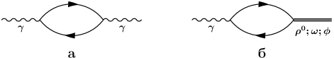
Figure 1: Divergent quark loops with external photons and vector mesons $\rho^{0}$, $\omega$, $\phi$.

After calculation of the divergent self-energy diagram of the photon (Fig. 1a), we obtain for $\mathcal{L}_{em}$ the expression

$$\mathcal{L}_{em}=-\frac{1}{4}(F_{\mu\,\nu}^{\prime})^{2}-i\mathrm{Tr}\ln\left[1-\frac{e}{i\hat{\partial}-M}Q\hat{A}\right]^{\prime},$$ (39)

where

$$A_{\mu}^{\prime}=\left(1+\frac{4}{3}\frac{e^{2}}{g_{\rho}^{2}}\right)^{1/2}A_{\mu}^{\prime},\quad e^{\prime}=\left(1+\frac{4}{3}\frac{e^{2}}{g_{\rho}^{2}}\right)^{-1/2}e$$ (40)

Besides the self-energy diagrams involving the photon there are divergent diagrams of mixed type, describing the transitions $\gamma\rho^{0}$, $\gamma\omega$ and $\gamma\phi$. (Fig. 1b). The inclusion of these diagrams leads to the appearance in the Lagrangian of terms of the form

$$\frac{1}{2}\frac{e^{\prime}}{g_{\rho}}F_{\mu\,\nu}^{\prime}\left(\rho^{0}_{\mu\,\nu}+\frac{1}{3}\omega_{\mu\,\nu}+\frac{\sqrt{2}}{3}\phi_{\mu\,\nu}\right),$$ (41)

where $\rho^{0}_{\mu\,\nu}$, $\omega_{\mu\,\nu}$ and $\phi_{\mu\,\nu}$ are tensors constructed from meson fields and derivatives, similarly to eq. (38).

As a result, the part of the Lagrangian that describes the electromagnetic interactions of the mesons and quarks takes the form

$$\mathcal{L}_{em} = \frac{M_{\rho}^{2}}{2}(\omega_{\mu}^{2}+\rho^{0}_{\mu})^{2}+\frac{M_{\phi}^{2}}{2}\phi_{\mu}^{2}-\frac{1}{4}\left({\rho^{0}}^{2}_{\mu\,\nu}+\omega_{\mu\,\nu}^{2}+\phi_{\mu\,\nu}^{2}+{F^{\prime}}^{2}_{\mu\,\nu}\right)$$

$$+\frac{1}{2}\frac{e^{\prime}}{g_{\rho}}F_{\mu\,\nu}^{\prime}\left(\rho^{0}_{\mu\,\nu}+\frac{1}{3}\omega_{\mu\,\nu}+\frac{\sqrt{2}}{3}\phi_{\mu\,\nu}\right)$$

$$-i\mathrm{Tr}\ln\left[1+\frac{1}{i\hat{\partial}-M}\left(\frac{g_{\rho}}{2}(\gamma_{\mu}\lambda^{i}V^{i}_{\mu})-e^{\prime}Q\hat{A}\right)\right]^{\prime},$$

where $V^{i}_{\mu}$ are the fields of vector mesons.

We diagonalize the kinetic terms by means of the following substitution of the fields:

$$\rho^{0}_{\mu}=\tilde{\rho}^{0}_{\mu}+\frac{e^{\prime}}{g_{\rho}}A^{\prime}_{\mu},\quad\omega_{\mu}=\tilde{\omega}_{\mu}+\frac{e^{\prime}}{3g_{\rho}}A^{\prime}_{\mu},\quad\phi_{\mu}=\tilde{\phi}_{\mu}+\frac{\sqrt{2}e^{\prime}}{3g_{\rho}}A^{\prime}_{\mu}$$ (43)

The electromagnetic field and the charge $e^{\prime}$ are then renormalized as follows:

$$\tilde{A}_{\mu} = \left(1-\frac{4}{3}\frac{{e^{\prime}}^{2}}{g_{\rho}^{2}}\right)^{1/2}A_{\mu}^{\prime},$$ (44)

$$\tilde{e} = \left(1-\frac{4}{3}\frac{{e^{\prime}}^{2}}{g_{\rho}^{2}}\right)^{-1/2}e^{\prime}=\left[\left(1-\frac{4}{3}\frac{{e^{\prime}}^{2}}{g_{\rho}^{2}}\right)\left(1+\frac{4}{3}\frac{e^{2}}{g_{\rho}^{2}}\right)\right]^{-1/2}e\rightarrow\tilde{e}=e$$

It is readily seen that as a result of the two renormalizations [ (39) and (44) ] the electric charge takes its original value. The final Lagrangian has the form

$$\mathcal{L}_{em} = \frac{M_{\rho}^{2}}{2}(\tilde{\omega}_{\mu}^{2}+\tilde{\rho}^{0}_{\mu})^{2}+\frac{M_{\phi}^{2}}{2}\tilde{\phi}_{\mu}^{2}-\frac{1}{4}\left({{\tilde{\rho^{0}}}_{\mu\,\nu}}^{2}+\tilde{\omega}_{\mu\,\nu}^{2}+\tilde{\phi}_{\mu\,\nu}^{2}+{{\tilde{F^{\prime}}}}^{2}_{\mu\,\nu}\right)$$ (45)

$$+\left(\frac{e}{3g_{\rho}}\right)^{2}\left(5M_{\rho}^{2}+m_{\phi}^{2}\right)\tilde{A}^{2}_{\mu}+\frac{e}{g_{\rho}}\left[M_{\rho}^{2}\left(\tilde{\rho^{0}}_{\mu}+\frac{\tilde{\omega}_{\mu}}{3}\right)+\frac{\sqrt{2}}{3}M_{\phi}^{2}\tilde{\phi}_{\mu}\right]$$

$$\qquad-i\mathrm{Tr}\ln\left[1+\frac{1}{i\hat{\partial}-M}\frac{g_{\rho}}{2}(\gamma_{\mu}\lambda^{i}V^{i}_{\mu})\right]$$

It is now easy to show that the photons can interact with the charged particles only through the neutral vector mesons. In this way, we have automatically obtained a model describing vector dominance. Under the sign of the logarithm, the term with photons has been completely absorbed by the vector mesons.

5 Meson in hot and dense matter

In the last few years the activity in search for a new state of matter, the quark-gluon plasma (QGP), has significantly increased. New data are already coming from running experiments on heavy-ion collisions at Brookhaven (RHIC) and CERN SPS. New facilities are planned to be constructed to increase our capability in this research (LHC, SIS-300). The QGP is expected to reveal itself through modified properties of hadronic reactions and their products.

The NJL model is a very convenient tool for investigation meson behavior in the hot and dense matter. First calculations of this type in NJL model were started in [11, 12].

It is possible to use different methods for investigation of meson behavior in the hot and dense matter. The most popular one is the Matsubara technique [28]. This ”imaginary time” formalism implies the replacement of the integration over the zero component of the momentum by the summation of frequencies

$$p^{0} \to (i\omega_{n}+\mu)$$ (46)

$$\int\frac{d^{4}p}{(2\pi)^{4}} \to iT\sum\limits_{n}\int\frac{d^{3}p}{(2\pi)^{3}},$$ (47)

where $\omega_{n}$ are the Matsubara frequencies, $\omega_{n}=(2n+1)\pi T$ for fermions and $\omega_{n}=2n\pi T$ for bosons; $\mu$ is the chemical potential and $T$ is the temperature.

However, for many applications it is more convenient to use an equivalent representation for the quark propagator derived in the ”real time” formalism [29]

$$S(p,T,\mu) = (\hat{p}+m)\left[\frac{1}{p^{2}-m^{2}+i\epsilon}+\right.$$ (48)

$$\left.i2\pi\delta(p^{2}-m^{2})(\theta(p^{0})n(\vec{p},\mu)+\theta(-p^{0})n(\vec{p},-\mu))\right],$$

where

$$n(\vec{p},\mu)=\left(1+\exp\frac{E-\mu}{T}\right)^{-1}$$ (49)

is the Fermi-Dirac function for quarks, $E=\sqrt{\vec{p}^{2}+m^{2}}$. This leads to a different method for calculation of integrals $I_{1}^{\Lambda_{3}}(m,T,\mu)$, $I_{2}^{\Lambda_{3}}(m,T,\mu)$. First we performed contour integration in the complex $p_{0}$ plane and after that reguralized integrals by three-momentum cut-off $\Lambda_{3}$. As a result, divergent integrals $I_{1}^{\Lambda_{3}}(m,T,\mu)$ and $I_{2}^{\Lambda_{3}}(m,T,\mu)$ take the form

$$I_{1}^{\Lambda_{3}}(m,T,\mu) = \frac{N_{c}}{(2\pi)^{2}}\int\limits_{0}^{\Lambda_{3}}dp\frac{p^{2}}{E}\left(1-\eta(\vec{p},\mu)-\tilde{\eta}(\vec{p},\mu)\right),$$

$$I_{2}^{\Lambda_{3}}(m,T,\mu) = \frac{N_{c}}{2(2\pi)^{2}}\int\limits_{0}^{\Lambda_{3}}dp\frac{p^{2}}{E^{3}}\left(1-\eta(\vec{p},\mu)-\tilde{\eta}(\vec{p},\mu)\right).$$ (50)

We defined values of model parameters in vacuum using the same conditions as in Sect. 2.4. Here we assume that model parameters $G_{\pi}$, $G_{\rho}$, $m_{0}$ and $\Lambda_{3}$ do not depend on $T$ and $\mu$. The dependence of $m$ on $T$ and $\mu$ is calculated from the gap equation. Then we calculate $T$ and $\mu$ dependence of basic integrals $I_{1}^{\Lambda_{3}}(m,T,\mu)$ and $I_{2}^{\Lambda_{3}}(m,T,\mu)$. This allows us to define the dependence on $T$ and $\mu$ of all physical quantities.

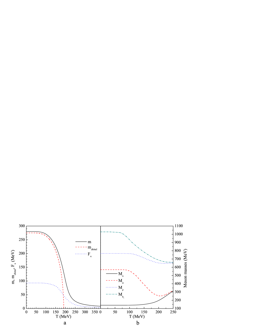
Figure 2: The behaviour of the quark mass and weak pion decay constant $F_{\pi}$ (a), and meson masses $M_{\pi}$, $M_{\sigma}$, $M_{\rho}$, $M_{a_{1}}$ (b) as function of $T$.

The behaviour of $m(T)$ is shown in Fig.2a. For $m_{0}=0$ the restoration of chiral symmetry is indicated by the vanishing of the order parameter $m(T)\to 0$ (or quark condensate) at critical value of the temperature $T_{c}$. When $m_{0}\neq 0$ the sharp phase boundary disappears. Figure 2b exhibits the behaviour of the meson masses $M_{\pi}$, $M_{\sigma}$, $M_{\rho}$, $M_{a_{1}}$ as function of $T$. As $T$ increases the mass of the $\sigma$ meson decreases sharply with the constituent quark mass. On the other hand, the mass of the pion will persistently stay constant until the critical conditions for chiral restoration are reached, beyond which it ceases to exist. $M_{\rho}$ is merely independent of $T$, whereas $M_{a_{1}}$ shows a sharp decrease similar to that of $M_{\sigma}$. Above the critical temperature one obtains $M_{\pi}=M_{\sigma}$ and $M_{\rho}=M_{a_{1}}$, as is expected for a chiral symmetric phase. In [30, 31] the value for critical temperature $T_{c}\approx 200$ MeV. In lattice recent QCD calculations the value for critical temperature $T_{c}\approx 170$ MeV [33].

Recently, very interesting results have been obtained from the investigation of strongly interacting quark matter in the color-superconducting phase. We do not consider here the diquark condensation and the related problems. The reader will find the details in [32, 34].

In conclusion, we would like to note that the properties of some particles can significantly change when approach to phase transition. The $\sigma$-meson, which in vacuum is a broad resonance may become very sharp resonance at particular temperature and chemical potential. When appropriate conditions are reached, this can lead to the amplification of some processes mediated by the $\sigma$-resonance, such as $\pi\pi\to\gamma\gamma$, $\pi\pi\to\pi\pi$ etc. This amplification, if observed in heavy-ion collision experiment, can be interpreted as an event indicating on the approaching the QGP.

6 First radial excitations of mesons

In the local version of the NJL model, it is impossible to describe radial excitations of mesons. Therefore, for the description of both the ground and first radially excited states it is necessary to consider not only the standard local Lagrangian $\mathcal{L}$ (1) but also additional nonlocal Lagrangian $\mathcal{L}^{\mathrm{nonloc}}$. In Lagrangian $\mathcal{L}^{\mathrm{nonloc}}$, we introduce a form-factor for each quark-antiquark current

$$J_{I}(x)=\int\int d^{4}x_{1}d^{4}x_{2}\,\bar{q}(x_{1})\,F_{I}(x;x_{1},x_{2})\,q(x_{2}).$$ (51)

The form-factors $F_{I}(x;x_{1},x_{2})$ can be written in a covariant form [35]. Here we do not discuss them in details, and only would like to remark the form-factors for the ground and first radially excited states can be given in a very simple form in momentum space,

$$f_{1}(k_{\bot}) = \Theta(\Lambda_{3}-|{k_{\bot}}|),$$ (52)

$$f_{2}(k_{\bot}) = c(1+d|{k_{\bot}}|^{2})\Theta(\Lambda_{3}-|{k_{\bot}}|),$$

where $k$ is the quark-antiquark pair relative momentum and $k_{\bot}$ is the part of $k$ transversal to the total momentum $P$

$$k_{\bot}\equiv k-\frac{k\cdot P}{P^{2}}P$$ (53)

The step function, $\Theta(\Lambda_{3}-|{k_{\bot}}|)$, is a covariant generalization of the 3-dimensional cut-off in the NJL model. For $d<-\Lambda_{3}^{-2}$ the form-factor $f_{2}(k_{\bot})$ has the form of an excited state wave function with a node in the interval $0<|{k_{\bot}}|<\Lambda_{3}$. The form-factors (52) are the first terms in a series expansion in ${k_{\bot}}^{2}$; the inclusion of higher radially excited states would require polynomials of a higher degree. The factor $c$ describes the change in the strength of the four-quark interaction in the radially excited channels relative to the constant $G_{\pi}$. This constant is defined from the mass of radial pion excitation $M_{\pi}^{\prime}=1300$ MeV. The parameter $d$ is defined from the condition

$$I_{1}^{f}=-iN_{c}\int_{\Lambda_{3}}\frac{d^{4}k}{(2\pi)^{4}}\frac{f_{1}(\mathbf{k})}{m^{2}-k^{2}}=0$$ (55)

Now let us explain the meaning of this condition. Note that in this model we have two gap equations

$$\frac{\delta\mathcal{W}}{\delta\sigma_{1}}=-iN_{c}\mathrm{tr}\int_{\Lambda_{3}}\frac{d^{4}k}{(2\pi)^{4}}\frac{1}{\hat{k}-m_{0}+\langle\sigma_{1}\rangle_{0}+\langle\sigma_{2}\rangle_{0}f_{2}(\mathbf{k})}-\frac{\langle\sigma_{1}\rangle_{0}}{G_{\pi}}=0$$ (56)

$$\frac{\delta\mathcal{W}}{\delta\sigma_{2}}=-iN_{c}\mathrm{tr}\int_{\Lambda_{3}}\frac{d^{4}k}{(2\pi)^{4}}\frac{f_{2}(\mathbf{k})}{\hat{k}-m_{0}+\langle\sigma_{1}\rangle_{0}+\langle\sigma_{2}\rangle_{0}f_{2}(\mathbf{k})}-\frac{\langle\sigma_{2}\rangle_{0}}{G_{\pi}}=0$$

In general, the solution of these equations would have $\langle\sigma_{2}\rangle_{0}\neq 0$; in this case the dynamically generated quark mass, $-\langle\sigma_{1}\rangle_{0}-\langle\sigma_{2}\rangle_{0}f_{1}(\mathbf{k})+m_{0}$, becomes momentum dependent. Condition (55) leads to the trivial solution for the second gap equation and, as a result, we have only one nontrivial gap equation coinciding with the standard gap equation of the local NJL model.

The free part of the effective action for pions takes the form

$$\mathcal{W}=\frac{1}{2}\int\frac{d^{4}P}{(2\pi)^{4}}\sum\limits_{i,j=1}^{2}\pi_{i}^{a}(P)K_{ij}^{ab}(P)\pi_{j}^{b}(P),$$ (57)

where $K_{ij}^{ab}(P)\equiv\delta^{ab}K_{ij}(P)$ and

$$K_{11}(P) = Z_{1}(P^{2}-M_{1}^{2}),\quad K_{22}(P)=Z_{2}(P^{2}-M_{2}^{2}),$$ (58)

$$K_{12}(P) = K_{21}(P)=\sqrt{Z_{1}Z_{2}}\Gamma P^{2},$$

with

$$M_{1}^{2} = \frac{1}{Z_{1}}\left(\frac{1}{G_{\pi}}-8I_{1}\right)=\frac{m_{0}}{Z_{1}G_{\pi}m},$$ (59)

$$M_{2}^{2} = \frac{1}{Z_{2}}\left(\frac{1}{G_{\pi}}-8I_{1}^{ff}\right),$$

$$Z_{1} = 4I_{2},\,Z_{2}=4I_{2}^{ff},\,\Gamma=\frac{4}{\sqrt{Z_{1}Z_{2}}}I_{2}^{f}.$$

To determine the physical $\pi$- and $\pi^{\prime}$-meson states, we have to diagonalize the quadratic part of the action. It can be performed with the help of an orthogonal tranformation of the fields $\pi_{1}$, $\pi_{2}$; the details of this procedure can be found in [35]. We would like to note that after the expansion in a series of a small current quark mass $m_{0}$ (from eq. (59) $M_{1}^{2}\sim m_{0}$), one finds for the physical states

$$M_{\pi}^{2} = M_{1}^{2}+O(M_{1}^{4}),$$ (60)

$$M_{\pi^{\prime}}^{2} = \frac{M_{2}^{2}}{1-\Gamma^{2}}\left[1+\Gamma^{2}\frac{M_{1}^{2}}{M_{2}^{2}}+O(M_{1}^{4})\right].$$

Thus, in the chiral limit, the effective Lagrangian indeed describes a massless Goldstone boson, the pion $\pi$, and a heavy pseudoscalar meson, $\pi^{\prime}$. The ratio of the $\pi$ and $\pi^{\prime}$ weak decay constants can be directly expressed in terms of the physical meson masses

$$\frac{F_{\pi^{\prime}}}{F_{\pi}} = \frac{\Gamma}{\sqrt{1-\Gamma^{2}}}\frac{M_{\pi}^{2}}{M_{\pi^{\prime}}^{2}}$$ (61)

It is worth noting that the matrix elements for a pseudoscalar meson and the divergence of the axial-vector current must vanish both for the pion and its radial excitation in the chiral limit. In the case of the pion, the matrix element is $\sim M_{\pi}^{2}$ and vanished in the chiral limit as $M_{\pi}^{2}\to 0$. The situation is opposite in the case of radially excited state, there $F_{\pi^{\prime}}\to 0$ in the chiral limit, while $M_{\pi^{\prime}}$ remaining finite.

Here we discuss only pions. In [36, 37, 38] it is shown that this method can be extended to the chiral $U(3)\times U(3)$ group for pseudoscalar, scalar and vector mesons. In the framework of this model the main strong decays of the radially excited meson were described [39, 37]. One of the most interesting results obtained in this model concerns the identification of nineteen experimentally observed scalar states for the masses 0.4 – 1.7 GeV. These states can be interpreted in our model as two scalar nonets and a scalar glueball with the mass $\sim 1.5$ GeV [40]. The first nonet consists of the ground state mesons with the masses between 0.4 – 1 GeV. The second nonet consists of radially excited scalar mesons with the masses 1.3 – 1.7 GeV. Four scalar states and scalar glueball are mixed, as they have the same quantum numbers.

7 Nonlocal NJL model and quark confinement

The NJL models have two main defects. They contain ultraviolet (UV) divergences and do not provide quark confinement. Usually, UV divergences are removed by using the cut-off parameter $\Lambda$ taken at an energy scale of the order of 1 GeV. The physical meaning of this cut-off is connected with the separation of the energy-momentum region, where spontaneous breaking of the chiral symmetry and bosonization of quarks takes place. In order to exclude unphysical quark-antiquark thresholds from amplitudes of different processes only lowest powers of momentum expansion of quark loops are usually used in the NJL models.

These drawbacks of the standard NJL model can be solved only in the framework of nonlocal models. There are many different nonlocal versions of NJL model (see e.g. [41, 42, 43, 44, 45]). Here we demonstrate one version of nonlocal models which is motivated by an instanton interaction [46]. Similar models are considered in [47, 48, 49, 50].

The $SU(2)\times SU(2)$ symmetric action with the nonlocal four-quark interaction has the form

$$\mathcal{S}(\bar{q},q)=\int d^{4}x\,\left\{\bar{q}(x)(i\hat{\partial}_{x}-m_{c})q(x)+\frac{G_{\pi}}{2}\left(J_{\sigma}(x)J_{\sigma}(x)+J_{\pi}^{a}(x)J_{\pi}^{a}(x)\right)\right.-$$

$$\left.-\frac{G_{\rho}}{2}(J_{\rho}^{\mu\,a}(x)J_{\rho}^{\mu\,a}(x)+J_{a_{1}}^{\mu\,a}(x)J_{a_{1}}^{\mu\,a}(x))\right\},$$ (62)

The nonlocal quark currents $J_{I}(x)$ are expressed as

$$J_{I}(x)=\int\int d^{4}x_{1}d^{4}x_{2}\,f(x_{1})f(x_{2})\,\bar{q}(x-x_{1})\,\Gamma_{I}\,q(x+x_{2}),$$ (63)

where the nonlocal function $f(x)$ is normalized by $f(0)=1$. In (62) the matrices $\Gamma_{I}$ are defined as $\Gamma_{\sigma}=\mathbf{1}$, $\Gamma_{\pi}^{a}=i\gamma^{5}\tau^{a}$, $\Gamma_{\rho}^{\mu\,a}=\gamma^{\mu}\tau^{a}$, $\Gamma_{a_{1}}^{\mu\,a}=\gamma^{5}\gamma^{\mu}\tau^{a}$.

After bosonization the scalar field $\sigma$ will have nonzero vacuum expectation value. In order to obtain a physical scalar field with zero vacuum expectation value, it is necessary to shift the scalar field. This leads to the appearance of the nonlocal quark mass $m(p^{2})$ instead of the current quark mass $m_{0}$ which can be found from the gap equation

$$m(p^{2}) = m_{0}+G_{\pi}\frac{2N_{c}}{(2\pi)^{4}}f^{2}(p^{2})\int d^{4}k\frac{f^{2}(k^{2})m(k^{2})}{k^{2}+m^{2}(k^{2})}=$$ (64)

$$= m_{c}+(m(0)-m_{c})f^{2}(p^{2}),$$

where $m(0)$ is the dimensional parameter which plays the role of the constituent quark mass. The quark propagator takes the form

$$S(p)=(\hat{p}-m(p^{2}))^{-1}.$$ (65)

We use one of the simplest $\mathrm{ans\ddot{a}tz}$ for the dynamically generated quark propagator. In the spirit of [41, 51] we demand that pole singularities are absent in the vector part of the quark propagator

$$\frac{1}{m^{2}(p^{2})+p^{2}}=\frac{1-\exp\left(-{p^{2}}/{\Lambda^{2}}\right)}{p^{2}}.$$ (66)

The expression for $m(p)$ is found to be:

$$m(p)=\left(\frac{p^{2}}{\exp\left({p^{2}}/{\Lambda^{2}}\right)-1}\right)^{1/2}.$$ (67)

The mass function $m(p^{2})$ depends only on one free parameter $\Lambda$, has no any singularities in the whole real axis and exponentially drops as $p^{2}\rightarrow\infty$ in the Euclidean domain. From eq.(64) it follows that nonlocal form factors have a similar behavior providing the absence of UV divergences in the model. At $p^{2}=0$ the mass function is equal to the cut-off parameter $\Lambda$, $m(0)=\Lambda$. From the gap equation we find the relation between the four-quark coupling $G_{1}$ and the nonlocality parameter $\Lambda$

$$G_{1}=\frac{2\pi^{2}}{N_{c}}\frac{1}{\Lambda^{2}}.$$ (68)

Moreover, the expression for pion renormalization constant has a simple form

$$g_{\pi}^{-2}(0)=\frac{N_{c}}{4\pi^{2}}\left(\frac{3}{8}+\frac{\zeta(3)}{2}\right)$$ (69)

where $\zeta$ is the Riemann zeta function. In the chiral limit one has two arbitrary parameters $\Lambda$, $G_{2}$. We fix their values with the help of the weak pion decay constant $F_{\pi}=93$ MeV, and $\rho$-meson mass $M_{\rho}=770$ MeV. By using the Goldberger-Treiman relation $g_{\pi}(0)=m(0)/F_{\pi}$ one finds $\Lambda=m(0)=340$ MeV.

This simple model leads to reasonable predictions for the $\sigma$-meson mass $M_{\sigma}=420$ MeV and strong decay $\rho\to\pi\pi$ $\Gamma_{\rho\pi\pi}=135\,\mathrm{MeV}$.

Nonlocal model, in contrast with the local NJL model, can be successfully used for the description of not only the constant part of amplitudes of meson interactions but also of the momentum dependence of amplitudes at small energies. It is worth noting that in the nonlocal model the relative contributions to the pion form-factor $F_{\gamma^{\ast}\pi^{+}\pi^{-}}$ and pion radii from the contact diagrams and diagrams with vector mesons as intermediate states have reasonable values [52]. In the nonlocal model the contribution of vector mesons is noticeably smaller than that of the contact diagrams in contrast with the local NJL model where these contributions are comparable [53]. The vector-meson diagrams play a very important role in the description of the pion form-factor $F_{\gamma^{\ast}\pi^{+}\pi^{-}}$ in the time-like region. These diagrams allow us not only to describe the $\rho$-meson resonance but also to obtain a correct behavior of the process form-factor in the region below 1 GeV.

8 Conclusion

Once more emphasize that when the first version of the NJL model was proposed, the fundamental theory of strong interactions QCD did not exist. Therefore, that time different versions of the phenomenological hadron models were used for description of low-energy hadron physics, whereas the description of hadron interactions at large energies was very problematic. However, after the construction of QCD and the discovery of the phenomenon of asymptotic freedom it became possible to describe an interaction of hadrons at large energies by means of perturbation theory. The perturbation theory is applicable only for energies larger than $1$ GeV when the strong coupling constant is smaller than unity. Therefore, for description of the low-energy region the usage of different phenomenological models is again needed.

One of the most attractive models of that kind is the NJL model. The basis of the model is the chiral symmetry of strong interactions(as in QCD). The region of applicability of this model supplements the QCD perturbation theory. The joint application of both the QCD theory and the NJL model allows us to consider the whole energy region of the strong hadron interactions.

M.K. Volkov is grateful to all collaborators (especially to D. Ebert) who took part in the construction and development of the NJL model.

The work is supported by RFBR grant 05-02-16699.

References

• [1] Y. Nambu and G. Jona-Lasinio, Phys. Rev.  122, 345 (1961).
• [2] V.G. Vaks and A.I. Larkin, Sov. Phys. JETP  13, 192 (1961).
• [3] B.A. Arbuzov, A.N. Tavkhelidze and R.N. Faustov, Dokl. Akad. Nauk SSSR   139, 345 (1961) [Sov. Phys. Dokl.  6, 598 (1962)].
• [4] T. Eguchi, Phys. Rev. D 14, 2755 (1976).
• [5] K. Kikkawa, Prog. Theor. Phys.  56, 947 (1976).
• [6] M. K. Volkov and D. Ebert, Yad. Fiz.  36, 1265 (1982).
• [7] D. Ebert and M. K. Volkov, Z. Phys. C 16, 205 (1983).
• [8] M. K. Volkov, Ann. Phys.  157, 282 (1984).
• [9] M. K. Volkov, Fiz. Elem. Chastits Atom. Yadra  17, 433 (1986).
• [10] D. Ebert and H. Reinhardt, Nucl. Phys. B 271, 188 (1986).
• [11] T. Hatsuda and T. Kunihiro, Phys. Lett. B 145, 7 (1984).
• [12] T. Hatsuda and T. Kunihiro, Phys. Rev. Lett.  55, 158 (1985).
• [13] U. Vogl and W. Weise, Prog. Part. Nucl. Phys.  27, 195 (1991).
• [14] T. I. Gulamov and A. I. Titov, Phys. Atom. Nucl.  58, 290 (1995).
• [15] S. Eidelman et al. [Particle Data Group], Phys. Lett. B 592, 1 (2004).
• [16] M. K. Volkov, A. N. Ivanov, M. Nagy and N. Troitskaya, Int. J. Mod. Phys. A 4, 3193 (1989).
• [17] M. K. Volkov and A. A. Osipov, Theor. Math. Phys.  86, 265 (1991).
• [18] V. Bernard, A. H. Blin, B. Hiller, Y. P. Ivanov, A. A. Osipov and U. G. Meissner, Annals Phys.  249, 499 (1996).
• [19] G. ’t Hooft, Phys. Rev. Lett.  37, 8 (1976).
• [20] S. Klimt, M. Lutz, U. Vogl and W. Weise, Nucl. Phys. A 516, 429 (1990).
• [21] S. P. Klevansky, Rev. Mod. Phys.  64, 649 (1992).
• [22] M. K. Volkov, Fiz. Elem. Chastits Atom. Yadra  24, 81 (1993).
• [23] D. Ebert, H. Reinhardt, and M. K. Volkov, Prog. Part. Nucl. Phys.  33, 1 (1994).
• [24] M. K. Volkov, M. Nagy and V. L. Yudichev, Nuovo Cim. A 112, 225 (1999).
• [25] R. L. Jaffe, Phys. Rev. D 15, 267,281 (1977).
• [26] N. N. Achasov, Nucl. Phys. A 728, 425 (2003).
• [27] S. B. Gerasimov, Nucl. Phys. Proc. Suppl.  126, 210 (2004).
• [28] J. I. Kapusta,Finite Temperature Field Theory (Cambridge Univ. Press, 1989).
• [29] L. Dolan and R. Jackiw, Phys. Rev. D 9, 3320 (1974).
• [30] D. Ebert, Y. L. Kalinovsky, L. Munchow and M. K. Volkov, Int. J. Mod. Phys. A 8, 1295 (1993).
• [31] T. Hatsuda and T. Kunihiro, Phys. Rep.  247, 221 (1994)
• [32] M. Buballa, Phys. Rept.  407, 205 (2005).
• [33] C. Bernard et al. [MILC Collaboration], Phys. Rev. D 71, 034504 (2005).
• [34] D. Blaschke, D. Ebert, K. G. Klimenko, M. K. Volkov and V. L. Yudichev, Phys. Rev. D 70, 014006 (2004).
• [35] M. K. Volkov and C. Weiss, Phys. Rev. D 56, 221 (1997).
• [36] M. K. Volkov, Phys. Atom. Nucl.  60, 1920 (1997).
• [37] M. K. Volkov and V. L. Yudichev, Phys. Part. Nucl.  31, 282 (2000).
• [38] D. Ebert, M. Nagy, M. K. Volkov and V. L. Yudichev, Eur. Phys. J. A 8, 567 (2000).
• [39] M. K. Volkov, D. Ebert and M. Nagy, Int. J. Mod. Phys. A 13, 5443 (1998)
• [40] M. K. Volkov and V. L. Yudichev, Eur. Phys. J. A 10, 109 (2001).
• [41] G. V. Efimov and M. A. Ivanov, Fiz. Elem. Chastits Atom. Yadra  20, 1129 (1989).
• [42] A. A. Andrianov, and V. A. Andrianov, Int. J. Mod. Phys. A 8, 1981 (1993).
• [43] A. A. Andrianov, D. Espriu and R. Tarrach, Nucl. Phys. B 533, 429 (1998).
• [44] L. S. Celenza, B. Huang, H. S. Wang and C. M. Shakin, Phys. Rev. C 60, 025202 (1999).
• [45] L. S. Celenza, S. f. Gao, B. Huang, H. Wang and C. M. Shakin, Phys. Rev. C 61, 035201 (2000).
• [46] A. E. Radzhabov and M. K. Volkov, Eur. Phys. J. A 19, 139 (2004).
• [47] M. Buballa and S. Krewald, Phys. Lett. B 294, 19 (1992).
• [48] R.S. Plant and M.C. Birse, Nucl. Phys. A 628, 607 (1998).
• [49] I.V. Anikin, A.E. Dorokhov and L. Tomio, Phys. Part. Nucl.  31, 509 (2000).
• [50] A. Scarpettini, D. Gomez Dumm and N. N. Scoccola, Phys. Rev. D 69, 114018 (2004).
• [51] G. V. Efimov and M. A. Ivanov, The Quark Confinement Model Of Hadrons (IOP, Bristol, 1993).
• [52] A. E. Dorokhov, A. E. Radzhabov and M. K. Volkov, Eur. Phys. J. A 21, 155 (2004)
• [53] M.K. Volkov, Phys. Atom. Nucl.  60, 997 (1997).