Testing SUSY models of lepton flavor violation at a photon collider

Abstract

The loop level lepton flavor violating signals $\gamma\gamma\to\ell\ell^{\prime}\;(\ell=e,\mu,\tau,\ell\neq\ell^{\prime})$ are studied in a scenario of low-energy, R-parity conserving, supersymmetric see-saw mechanism within the context of a high energy photon collider. Lepton flavor violation is due to off diagonal elements in the left s-lepton mass matrix induced by renormalization group equations. The average slepton masses ${\widetilde{m}}$ and the off diagonal matrix elements $\Delta m$ are treated as model independent free phenomenological parameters in order to discover regions in the parameter space where the signal cross section may be observable. At the energies of the $\gamma\gamma$ option of the future high-energy linear collider the signal has a potentially large standard model background, and therefore particular attention is paid to the study of kinematical cuts in order to reduce the latter at an acceptable level. We find, for the ($e\tau$) channel, non-negligible fractions of the parameter space ($\delta_{LL}=\Delta m^{2}/\widetilde{m}^{2}\gtrsim 10^{-1}$) where the statistical significance ($SS$) is $SS\gtrsim 3$.

I Introduction

The high-energy linear lepton collider (LC) is presently considered as a necessary next step in the field of high-energy physics. If new physics will show up at the CERN Large Hadron Collider (LHC), a LC with a much cleaner environment would allow unambiguous precision measurements. However the LC project has the potential to address, on its own, questions of physics beyond the standard model, since $e^{-}e^{-}$ and $\gamma\gamma$ options are also planned beside the basic $e^{+}e^{-}$ mode. If these options are carried on, they will provide us for the first time with the high physics potential of very high-energy $e^{-}e^{-}$ and $\gamma\gamma$ collisions. See for example ILC for a full discussion of the physics potential of the TESLA photon collider (PC).

A topic which has recently received considerable attention is that of neutrino mass and lepton number (flavor) violation, LNV (LFV). Non-vanishing neutrino masses induce LFV processes such as $\ell\rightarrow\ell^{\prime}\gamma$. If neutrinos have masses in the eV or sub-eV range, the neutrino generated branching ratio to the latter process is of order ${\cal O}$(10^-40) and therefore unobservably small. For such processes to be experimentally accessible, new physics has to come into play. Experimental searches of radiative lepton decays put strong bounds on models of LFV: $Br(\mu\to e\gamma)<1.2\times 10^{-11}$ mue , $Br(\tau\to e\gamma)<3.9\times 10^{-7}$ taue , $Br(\tau\to\mu\gamma)<3.1\times 10^{-7}$ taumu . Supersymmetric (SUSY) extensions of the SM in the soft SUSY breaking potential $V_{soft}$ contains, in general, non diagonal entries in generation space and therefore additional potential sources for LFV. Even in minimal supergravity scenarios characterized by universal soft mass term for scalar slepton and squark fields, renormalization induces potentially sizable weak scale flavor mixing Gabbiani in $V_{soft}$.

In this paper we study the lepton flavor violating reaction

$${\gamma\gamma\to\ell{\ell^{\prime}}}$$ (1)

with $\ell\neq\ell^{\prime}$ and $\ell,\ell^{\prime}=e,\mu,\tau$, which arises at one loop order in the just mentioned SUSY scenario, thus extending to the $\gamma\gamma$ option an analysis done by some of the authors in Ref. cannoni for the $e^{+}e^{-}$ and $e^{-}e^{-}$ mode of the next linear collider. The OPAL collaboration searched for this type of LFV reactions up to the highest center-of-mass (CM) energy reached by LEPII, $\sqrt{s}=209$ GeV opal . One $e^{+}e^{-}\to e\mu$ event was found at $\sqrt{s}=189$ GeV matching all tagging conditions, but it was interpreted as due to initial state radiation. These processes have the advantage of providing a clean final state which is easy to identify experimentally (two back-to-back different flavor leptons), though one has to pay the price of dealing with cross sections of order ${\cal O}(\alpha^{4})$. In Ref. cannoni we found that the $e^{-}e^{-}$ option stands better perspectives for the possible detection of a LFV signal as opposed to the $e^{+}e^{-}$ mode, both because of larger cross sections and smaller background. In general the $\gamma\gamma$ mode offers larger cross section as compared to the other modes, but at the same time has the drawback of larger background and one must take into account the non-monochromaticity of the beams.

The plan of the paper is the following: in section II we discuss the SUSY scenario of LFV in the charged slepton sector (details of the helicity amplitudes of the diagrams contributing to the signal reactions are given in the appendix); in section III we review briefly the photon spectra used in the numerical computations of the signal ; in section IV we discuss the main features of the signal; in section V we discuss the main standard model (SM) backgrounds, and finally in section VI we present the concluding remarks.

II SUSY scenario for lepton flavor violation

In the SUSY extension (with mSUGRA boundary conditions) of the seesaw mechanism for the explanation of neutrino masses borma , the superpotential contains three $SU(2)_{L}$ singlet neutrino superfields $N_{i}$ with the following couplings borma ; hisa2 ; hisa3 :

$$W=(Y_{\nu})_{ij}\varepsilon_{\alpha\beta}H_{2}^{\alpha}N_{i}L^{\beta}_{j}+\frac{1}{2}(M_{R})_{i}N_{i}N_{i}.$$ (2)

Here $H_{2}$ is a Higgs doublet superfield, $L_{i}$ are the $SU(2)_{L}$ doublet lepton superfields, $Y_{\nu}$ is a Yukawa coupling matrix and $M_{R}$ is the $SU(2)_{L}$ singlet neutrino mass matrix. At low energy the renormalization group equations (RGE) produce within the MSSM diagonal slepton mass matrices. With the additional Yukawa couplings in Eq. (2) and the new mass scale ($M_{R}$) the RGE evolution of the soft SUSY breaking parameters is modified : assuming a heavy right handed singlet neutrino mass scale, $M_{R}$, the RGE from the GUT scale down to $M_{R}$ induce off-diagonal matrix elements in $(m^{2}_{\tilde{L}})_{ij}$. In the one loop approximation the off-diagonal elements are hisa2 :

$$(m^{2}_{\tilde{L}})_{ij}\simeq-\frac{1}{8\pi^{2}}(3+a^{2}_{0})m_{0}^{2}(Y_{\nu}^{\dagger}Y_{\nu})_{ij}\ln\left(\frac{M_{GUT}}{M_{R}}\right).$$ (3)

$a_{0}$ is a dimensionless parameter appearing in the matrix of trilinear mass terms $A_{\ell}=Y_{\ell}a_{0}m_{0}$ contained in $V_{soft}$. The rate of LFV transitions like $\ell_{i}\to\ell_{j}$, $i\neq j$, $\ell=e,\mu,\tau$ induced by the lepton-slepton-gaugino vertex is determined by the diagonalization matrix ${U_{L}}_{ij}$. These matrix elements can be potentially large because they are not directly related to the mass of the light neutrinos, but only through the seesaw relation $m_{\nu}\simeq m^{2}_{D}/M_{R}=v^{2}Y^{2}_{\nu}/M_{R}$. The same effect on the mass matrix of $SU(2)_{L}$ singlet charged sleptons $(m^{2}_{\tilde{R}})_{ij}$ is instead much smaller : indeed, in the same leading-log approximation of Eq. (3), the corresponding RGE do not contain terms proportional to $Y_{\nu}^{\dagger}Y_{\nu}$, since the right-handed leptons fields only have the Yukawa coupling $Y_{\ell}$, which completely determines the Dirac mass of the charged leptons and these are known to be small numbers. Thus the off-diagonal elements of $(m^{2}_{\tilde{R}})_{ij}$ can be taken to a vanishing to a very good degree of accuracy. The mixing matrix arising in the diagonalization of $(m^{2}_{\tilde{L}})_{ij}$ induce LFV couplings in the lepton-slepton-gaugino vertices $\tilde{\ell}^{\dagger}_{L_{i}}{U_{L}}_{ij}\tilde{\ell}_{L_{j}}\chi$. The magnitude of LFV effects will in turn depend on the fundamental theory in which this mechanism is embedded (for example $SU(5)$ or $SO(10)$ SUSY GUT hisa3 ; biqi ; masiso10 ) and on the particular choice of texture for the neutrinos mass matrix casas ; ellis ; pas .

In this paper we adopt a more general and phenomenological approach, as it was done in cannoni , without referring to a particular GUT model or neutrino mass texture. We consider a two generation model for the mass matrix of left-sleptons (and sneutrinos):

$$\widetilde{m}^{2}_{{L}}=\left(\begin{array}[]{cc}\widetilde{m}^{2}&\Delta m^{2}\\ \Delta m^{2}&\widetilde{m}^{2}\end{array}\right),$$ (6)

with eigenvalues: $\widetilde{m}^{2}_{\pm}=\widetilde{m}^{2}\pm\Delta m^{2}$ and maximal mixing. Under these assumptions, the lepton flavor violating propagator (in momentum space) for a scalar line is

$$\langle\tilde{\ell}_{i}\tilde{\ell}^{\dagger}_{j}\rangle_{0}=\frac{i}{2}\left(\frac{1}{p^{2}-\widetilde{m}^{2}_{+}}-\frac{1}{p^{2}-\widetilde{m}^{2}_{-}}\right)=i\frac{\Delta m^{2}}{(p^{2}-\widetilde{m}^{2}_{+})(p^{2}-\widetilde{m}^{2}_{-})}\ ,$$ (7)

while the propagator for a lepton flavor conserving (LFC) scalar line is:

$$\langle\tilde{\ell}_{i}\tilde{\ell}^{\dagger}_{i}\rangle_{0}=\frac{i}{2}\left(\frac{1}{p^{2}-\widetilde{m}^{2}_{+}}+\frac{1}{p^{2}-\widetilde{m}^{2}_{-}}\right).$$ (8)

The quantity

$$\delta_{LL}={\Delta m^{2}}/{\widetilde{m}^{2}}$$ (9)

is the dimension-less parameter that controls the magnitude of the LFV effect. This approach allows us to study the signal in a quite model-independent way by means of scans in the parameter space – the ($\widetilde{m},\delta_{LL}$) plane – which is already constrained by the experimental bounds on radiative lepton decay processes.

For the calculations presented in this work it is a good approximation to assume that the two lightest neutralinos are pure Bino and pure Wino with masses $M_{1}$ and $M_{2}$ respectively, while charginos are pure charged Winos with mass $M_{2}$, $M_{1}$ and $M_{2}$ being the gaugino masses in the soft breaking potential. The Higgsino contribution to neutralino and charginos has suppressed amplitude, since the coupling is proportional to the lepton masses. For the same reason left-right mixing in the slepton matrix is neglected. The relevant parts of the interaction lagrangian are, adopting the notation of Haber :

$${\cal L}=-g\overline{\ell}P_{R}\widetilde{W}\tilde{\nu}+\frac{g}{\sqrt{2}}\overline{\ell}P_{R}\widetilde{W}^{3}\tilde{\ell}_{L}+\frac{g}{\sqrt{2}}t_{W}\overline{\ell}P_{R}\tilde{B}\tilde{\ell}_{L}+e\tilde{\ell}_{L}A_{\mu}\tilde{L}^{*}i\overleftrightarrow{\partial}^{\mu}\tilde{\ell}_{L}-eA_{\mu}\overline{\widetilde{W}}\gamma^{\mu}\widetilde{W}$$ (10)

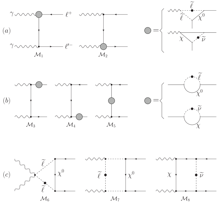
The contributing one loop diagrams are displayed in Figure 1. We have grouped them according to their topology : (a) penguin type ; (b) self-energy ; (d) box diagrams. It is of course understood that each diagram is accompanied by an exchange diagram where the final state leptons (or initial state photons) are exchanged.

The possibility of having, at the next LC, high-energy polarized photon beams suggests (see discussion in section III) to calculate the amplitudes of the diagrams in Fig. 1 within the helicity formalism. Denoting by $\hat{T}$, $\hat{X}$, $\hat{Y}$, $\hat{Z}$ the space-time unit four-vectors, the four-momenta of the particles in the center-of-mass frame (CMF) are expressed as:

$$\begin{array}[]{ll}\displaystyle p_{1}=\frac{\sqrt{s}}{2}\left(\hat{T}+\hat{Z}\right)&\displaystyle\qquad p_{3}=\frac{\sqrt{s}}{2}\left(\hat{T}+\hat{X}\sin\theta^{*}+\hat{Z}\cos\theta^{*}\right)\\ \displaystyle p_{2}=\frac{\sqrt{s}}{2}\left(\hat{T}-\hat{Z}\right)&\displaystyle\qquad p_{4}=\frac{\sqrt{s}}{2}\left(\hat{T}-\hat{X}\sin\theta^{*}-\hat{Z}\cos\theta^{*}\right)\end{array}$$ (11)

where $s=(p_{1}+p_{2})^{2}$ and $\theta^{*}$ are, respectivley, the CMF energy and scattering angle, while the polarization four-vectors of the photons are:

$$\epsilon^{\lambda}_{1}=-\frac{1}{\sqrt{2}}\left(\lambda\hat{X}+i\hat{Y}\right)\qquad\epsilon^{{\lambda}^{\prime}}_{2}=+\frac{1}{\sqrt{2}}\left({\lambda}^{\prime}\hat{X}-i\hat{Y}\right),$$ (12)

where $\lambda$ and ${\lambda}^{\prime}$ ($=\pm 1$) denote the photon helicities. Assuming massless external fermions and, given the chiral nature of the coupling in the lagrangian, the helicity of the fermions in the final state are fixed to only one configuration, thus there are only four helicity amplitudes corresponding to the possible combinations of the photon helicities. With obvious notation, we indicate with ${\cal M}^{(\lambda,\lambda^{\prime})}$ the helicity amplitudes. The loop integrals are decomposed in form factors according to the notations of the software package LoopTools looptools which is used in the code for numerical computations. The final analytical formulas of the amplitudes ${\cal M}^{(\lambda,\lambda^{\prime})}$ are function of $s$, $\theta^{*}$, $\lambda$, ${\lambda}^{\prime}$ and the SUSY parameters. They also contain form factors originating from the loop integrals which are defined according to the LoopTools conventions. We report the explicit expressions of the helicity amplitudes in the Appendix A.

Figure 1: Diagrams for $\gamma\gamma$ collisions : $(a)$ penguin diagrams ; $(b)$ Self-energy diagrams ; $(c)$ box diagrams. The full black dot in a scalar line denotes the insertion of the lepton flavor violating propagator (Eq. 7). In the diagrams of part $(c)$ this insertion is to be done successively in each scalar line. In addition all graphs are accompanied by an exchange graph where the final leptons are interchanged.

III Discussion of photon beams and PC luminosity

High-energy photons beams Ginzburg1 ; ILC will be obtained from Compton back-scattered (CB) low-energy laser photons with energy $\omega_{0}$ off high-energy electron beams with energy $E_{0}$. These high-energy photon beams will not be monochromatic but will present instead an energy spectrum, mainly determined by the Compton cross section, up to a maximum energy $y_{m}E_{0}$, where $y_{m}=x/(x+1)$ with $x=4E_{0}\omega_{0}/m^{2}_{e}$.

Full simulations of the experimental apparatus, see for example the simulation of Telnov for TESLA telnov , show that the real luminosity spectrum cannot be described by simple analytical formulas because of energy-angle correlation in Compton scattering, collisions effects and details of the collision region. Besides the high-energy peak also a 5-8 times higher low-energy peak is present, which is originated by photons after multiple Compton scattering and beamstrahlung that cannot be described by analytical formulas.

The high-energy peak is instead found to be almost independent of the technological details and well reproduced by the product of two Compton spectra. The normalized Compton energy spectrum is:

$$F_{c}(x,y)\equiv\frac{1}{N_{c}}\frac{dN_{c}}{dy}=\frac{1}{N_{c}}\left[\frac{1}{1-y}-y+(2r-1)^{2}-\lambda_{e}\,P_{\ell}\,x\,r\,(2r-1)(2-y)\right]$$ (13)

where $N_{c}$ is the normalization constant , $y=E_{\gamma}/E_{0}$ is the fraction of the initial electron energy acquired by the CB photons, $r=y/x(1-y)$, and $\lambda_{e}$ and $P_{l}$ are the electrons and laser photons polarizations ($|\lambda_{e},P_{l}|\leq 1$), respectively. Thus the theoretical differential spectrum for luminosity is:

$$\frac{dL_{\gamma\gamma}^{CB}}{dy_{1}dy_{2}}=\,F_{c}(x,y_{1})\,F_{c}(x,y_{2}).$$ (14)

It is useful to rewrite Eq. (14) in terms of the invariant variables $z=\sqrt{y_{1}y_{2}}=W_{\gamma\gamma}/2E_{0}=\sqrt{s_{\gamma\gamma}/s_{ee}}$ and the pseudo-rapidity $\eta=\ln{\sqrt{y_{1}/y_{2}}}$, and define a differential spectrum as a function of $z$ :

$$\frac{dL_{\gamma\gamma}^{CB}}{dz}=2z\,\int^{\ln{y_{m}/z}}_{-\ln{y_{m}/z}}F_{c}(x,ze^{+\eta})F_{c}(x,ze^{-\eta})d\eta.$$ (15)

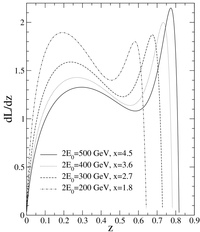
Figure 2: The ideal CB luminosity spectrum plotted for different CM energies of the $ee$ collider.

This is the function we have plotted in Fig. 2 for some values of $E_{0}$ and for correlated value of $x$ calculated using the TESLA parameter $\omega_{0}=1.17$ eV. It gives a peak of luminosity near the maximum value of $z$, $z_{m}=W_{\gamma\gamma\,\text{max}}/2E_{0}=y_{m}$, as shown in Fig. (2) and a broad spectrum at lower values. This means that most of the collisions involve two high-energy photons from the high-energy peaks of the two Compton spectra. We note that the peak in the luminosity spectrum is obtained when the product $P_{\ell}\,\lambda_{e}$ is negative for both Compton spectra.

In this high-energy range, the colliding photons have practically the same energy which is close to its maximum value. Obviously, this configuration is the most favourable to distinguish two-particle final states among multi-particle production. It is important to notice that the experimental design for a future photon-photon collider is planned so as to have full control of the luminosity and optimize it in this high-energy range in view of Higgs physics studies telnov . In the low-energy range, collisions between photons that may have very different energies take place, leading to copious boosted events. Then, the separation between signal and background becomes more challenging. Moreover, this low-energy part is more dependent of the experimental apparatus. For these reasons, we have restricted our study to the high-energy part of the luminosity spectrum. Another reason to restrict the peak is that the total luminosity of the photon collider is defined by the condition

$$L_{\gamma\gamma}=\int^{z_{max}}_{0.8z_{max}}dz\frac{dL_{\gamma\gamma}}{dz}.$$ (16)

To evaluate the expected total number of events and event rates we take as benchmark the TESLA parameters in Ref. ILC . At $\sqrt{s_{ee}}=2E_{0}=200$, $500$ GeV the geometrical luminosities are expected to be $L_{0}=$ ($4.8$, $12$, $19.1$)$\times 10^{34}$ cm^-2 s^-1, while the corresponding photon-photon luminosities at the peak are : $L_{\gamma\gamma}(z>0.8z_{m})=$(0.44, 1.15) $\times 10^{34}$ cm^-2 s^-1, equivalent to (1.3, 3.4) $\times$ 10² fb^-1 yr^-1. To use these simulated realistic numbers with the ideal spectrum in Eq. (15) a suitable normalization is necessary :

$$L_{\gamma\gamma}=C_{norm}\int^{z_{max}}_{0.8z_{max}}~{}2z~{}dz\,\int^{\ln{y_{m}/z}}_{-\ln{y_{m}/z}}F_{c}(x,ze^{+\eta})F_{c}(x,ze^{-\eta})d\eta.$$ (17)

$$N_{events}=L_{\gamma\gamma}\int^{z_{max}}_{0.8z_{max}}dz\frac{1}{L_{\gamma\gamma}}\frac{dL_{\gamma\gamma}}{dz}\sigma(W_{\gamma\gamma})$$ (18)

Substituting Eqs. (17,18) into the integral we eliminate the dependence from $C_{norm}$, which depends on the total integrated luminosity, redefining the differential spectrum as

$$\frac{dL^{norm}_{\gamma\gamma}}{dz}=L_{norm}\frac{dL^{CB}_{\gamma\gamma}}{dz},$$ (19)

where $L_{norm}$ is given by:

$$L_{norm} = \frac{1}{\int^{z_{max}}_{0.8z_{max}}dz2z\,\int^{\ln{y_{m}/z}}_{-\ln{y_{m}/z}}F_{c}(x,ze^{+\eta})F_{c}(x,ze^{-\eta})d\eta}$$ (20)

Thus we define both for signal and background the effective cross section as :

$$\sigma^{effective}=\int^{z_{max}}_{z_{min}}dz\frac{dL^{norm}_{\gamma\gamma}}{dz}\sigma(W_{\gamma\gamma})$$ (21)

and the total number of events is thus given by $N_{events}=L_{\gamma\gamma}\times\sigma^{effective}$.

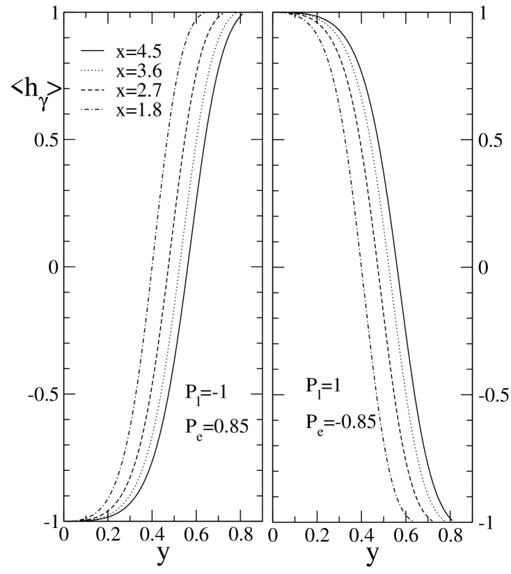
Figure 3: The ideal CB helicity spectrum plotted for different center of mass energies of the $ee$ collider.

In view of studying helicity correlations, we discuss the polarizations properties of the back-scattered photons. The degree of circular polarization is given by:

$$\langle h_{\gamma}\rangle=\frac{-P_{\ell}(2r-1)\left[(1-y)^{-1}+1-y\right]+2\lambda_{e}xr\left[1+(1-y)(2r-1)^{2}\right]}{N_{c}\;F_{c}(x,y)}$$ (22)

Assuming complete polarization for laser photons ($P_{\ell}=\pm 1$) and the planned maximum available for electrons $\lambda_{e}=\pm 0.85$, this function is plotted in Figure 3 for various values of $x$. As can be seen, in the high-energy peak where $y$ is near $y_{m}$, colliding photons have a high degree of circular polarization with $P_{\gamma}=-P_{l}$.

IV Discussion of the signal

We discuss first the signal for the ideal case with monochromatic photons in pure helicity state. The differential polarized cross sections with respect to the scattering angle in the photon-photon CMF are given by

$$\frac{d{\hat{\sigma}}^{\lambda\lambda^{\prime}}}{d\cos{\theta}^{*}}=\frac{1}{32\pi\hat{s}}\big{|}{\cal M}^{\lambda\lambda^{\prime}}(\hat{s},\hat{t},\hat{u})\big{|}^{2}\,.$$ (23)

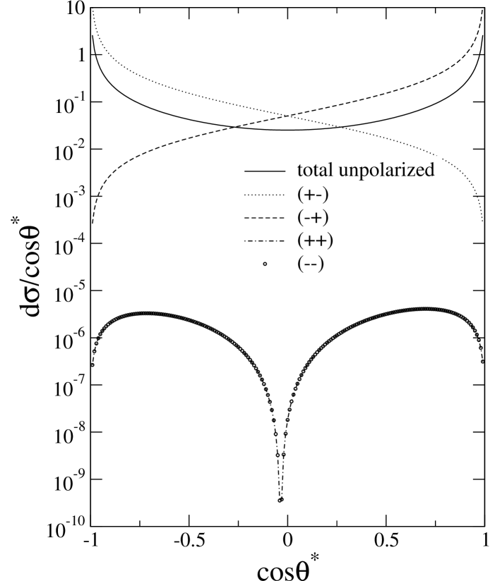
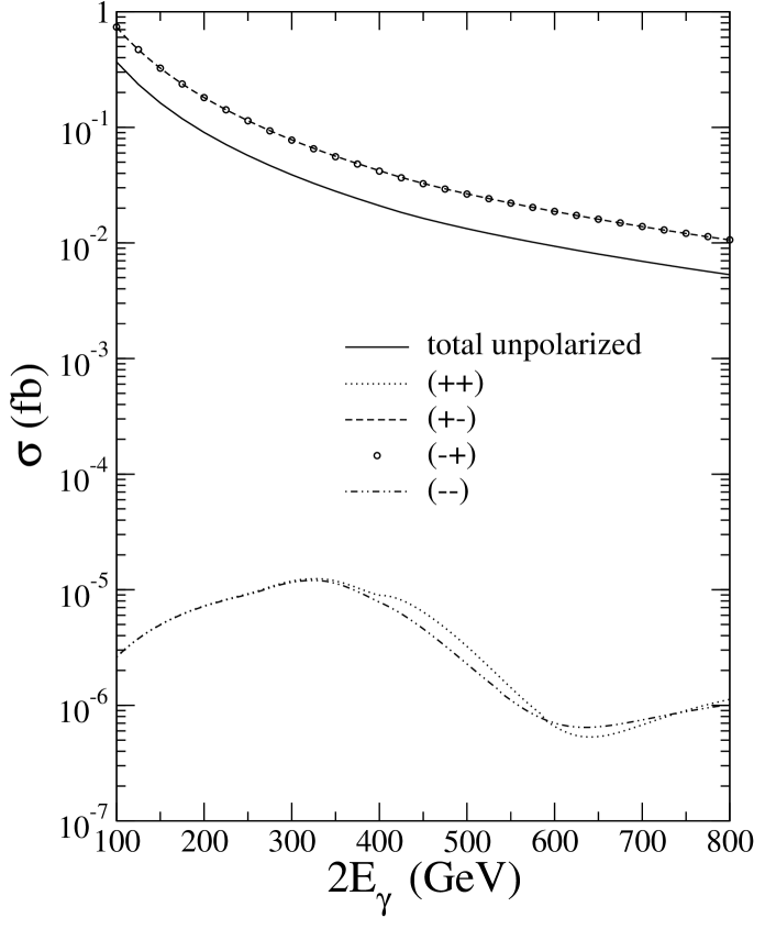
Figure 4: Differential cross section given by the four helicity amplitudes for monochromatic photons at $\sqrt{s_{\gamma\gamma}}=128$ GeV. The values of the masses are $M_{1}=200$, $M_{2}=100$, $\langle\tilde{m}_{l}\rangle=150$ GeV and $\Delta m^{2}=6000$ GeV².

We plot them in Figure 4 as functions of the CMF scattering angle with masses set to the values specified in the caption of the figure and for $\sqrt{s_{\gamma\gamma}}=128$ GeV which corresponds to the maximum energy that is reachable with a LC with $\sqrt{s_{ee}}=200$ GeV. It is seen that the amplitudes with opposite helicity photons ${\cal M}^{(+,-)}$ and ${\cal M}^{(-,+)}$ ($J_{z}=\pm 2$) dominate the signal, while those with same helicity photons ($J_{z}=0$) give negligible cross-sections. Moreover the former are peaked in the forward and backward directions while the second are suppressed in these regions.

Figure 5: Total signal cross sections for monochromatic photons as a function of the energy with the parameters as specified in the caption of Figure 4 .

The total cross sections are plotted in Figure 5 varying the CM energy. The $J_{z}=\pm 2$ cross sections decrease with increasing energy for they are dominated by the diagrams with the exchange of a light lepton in the $t$ and $u$ channels [(a) and (b) of Fig. 1].

The realistic effective differential cross sections as function of the scattering angle in the laboratory ($e^{-}e^{-}$ CMF) are simply obtained by a boost and by convoluting the “monochromatic” differential cross-sections in Eq. (23) with the luminosity spectrum discussed in the preceding section. The fact that photons are not in pure helicity state is here taken into account using density matrices for initial photons expressed in terms of Stokes parameters landau . The complete formula is:

$$\frac{d{{\sigma}}^{\lambda\lambda^{\prime}}}{d\cos{\theta}}=\int^{z_{max}}_{z_{min}}dz\,\,\frac{dL^{norm}_{\gamma\gamma}}{dz}\frac{d\cos{\theta}^{*}}{d\cos{\theta}}\frac{\left(1-\langle\lambda(x,P_{\ell_{1}},\lambda_{e_{1}})\rangle\right)}{2}\frac{\left(1-\langle\lambda^{\prime}(x,P_{\ell_{2}},\lambda_{e_{2}})\rangle\right)}{2}\frac{d{\hat{\sigma}}^{\lambda\lambda^{\prime}}}{d\cos{\theta}^{*}}$$ (24)

Here the functions $\langle\lambda(x,P_{\ell_{1}},\lambda_{e_{1}})\rangle$, $\langle\lambda^{\prime}(x,P_{\ell_{2}},\lambda_{e_{2}})\rangle$ play the role of the Stoke parameter $\eta_{2}$, while $\eta_{1}$ and $\eta_{3}$ landau give no contribution for we are assuming laser photons with full circular polarization. The total cross sections are obtained finally by integrating over the laboratory scattering angle and introducing a kinematical cut :

$$\sigma^{\lambda\lambda^{\prime}}(s_{ee})=\int^{(\cos\theta)_{max}}_{(\cos\theta)_{min}}d\cos\theta\,\frac{d{\hat{\sigma}}^{\lambda\lambda^{\prime}}}{d\cos{\theta}}$$ (25)

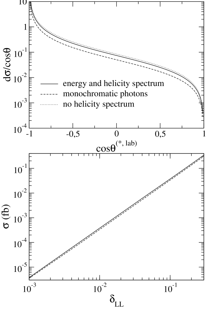
Figure 6: Effect of energy and helicity spectra on angular and total cross sections for the helicity configuration (+ -). The values of masses are the same as in Figures 4,  5.

In Figure 6 we study the effect of the inclusion of spectra in the calculation. The upper panel presents the same monochromatic (+ -) differential cross section of Figure 4 compared with the one calculated with the complete formula of Eq. 24, while the bottom panel shows the total cross section as a function of the parameter $\delta_{LL}$ (c.f. Eq. 9) : it is clear that the complete formula in Eq. 24 gives results almost identical (within a few $\%$) to the monochromatic calculation with photon energies fixed to their maximum values. This is a consequence of the choice of restricting the calculation to the luminosity peak near $z_{m}$ where the photons have energies near $E_{\gamma}^{max}$, are in an almost defined helicity state and the boost to the lab system has $\beta\simeq 0$. Thus, in the following we consider the cases of a photon collider with $2E_{0}=200$ and 500 GeV, with monochromatic photons in pure helicity states with $E_{\gamma}=E_{\gamma}^{max}$ ($\sqrt{s_{\gamma\gamma}}=128$ and 410 GeV respectively) and use the realistic simulated luminosities of TESLA to estimate event rates.

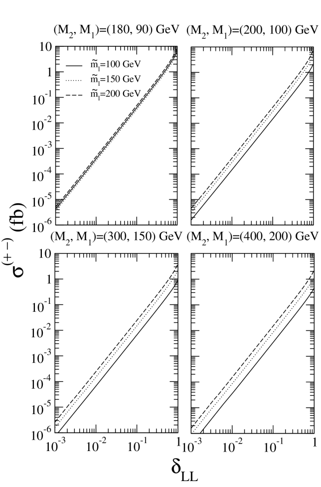
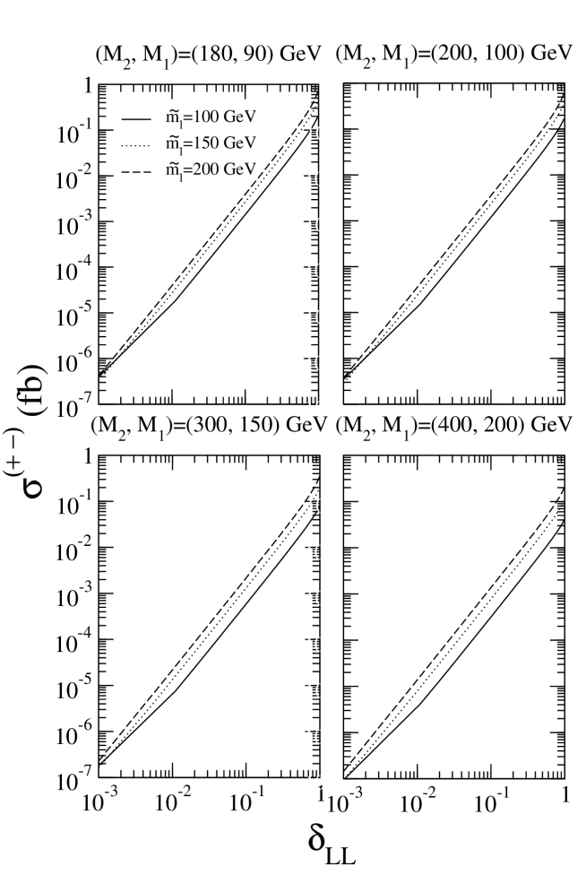
In Figures 7 and 8 we plot the cross section given by the dominant amplitude (+ -) as function of the insertion $\delta_{LL}$ for some values of gaugino and average slepton masses. These values are in the range of the SPS1 benchmark point mSUGRA scenario sps that give a particle spectrum with the lightest charginos, neutralinos and sleptons in the $100-200$ GeV region. This light spectrum is also favoured by global fits to the standard model parameters altarelli . Even if the differential cross section is peaked along the collision axis, a necessary angular cut $|\cos\theta|<0.9$ is applied because the background is also large in this region, as it is discussed in Section V. Given luminosities of order ${\cal O}(100)$ fb^-1yr^-1, cross sections greater than $10^{-2}$ fb are needed. In the case of a $2E_{0}=200$ GeV  PC, this happens for $\delta_{LL}>5\times 10^{-2}$ while in the $2E_{0}=500$ GeV case, $\delta_{LL}>5\times 10^{-1}$ is needed, which means quite large non-diagonal matrix elements.

Figure 7: Total cross section for the amplitude (+ -) as a function of the dimensionless parameter $\delta_{LL}$ and $\sqrt{s_{\gamma\gamma}}=128$ GeV. The values of the others parameters are given in the legends.

Figure 8: Total cross section for the amplitude (+ -) as a function of the dimensionless parameter $\delta_{LL}$ and $\sqrt{s_{\gamma\gamma}}=410$ GeV. The values of the others parameters are given in the legends.

To see if these large mass splittings are allowed by current experimental constraints we have to take into account the bounds imposed on the model by the non observation of radiative decays.

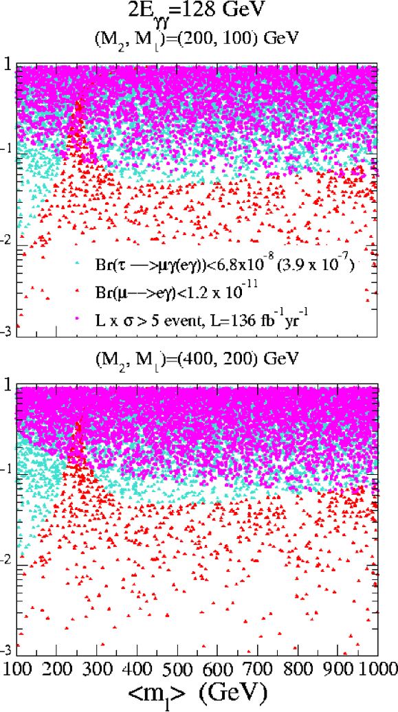
Figure 9: Scatter plot in the plane ($\delta_{LL},\widetilde{m}$) of: (a) the experimental bounds from $\mu\to e\gamma$ and $\tau\to\mu\gamma$ (allowed regions with circular dots); (b) regions where the signal can give at least five events at year for two sets of gaugino masses. The energy is $\sqrt{s_{\gamma\gamma}}=128$ GeV and the luminosity $L=136$ fb^-1 yr^-1.

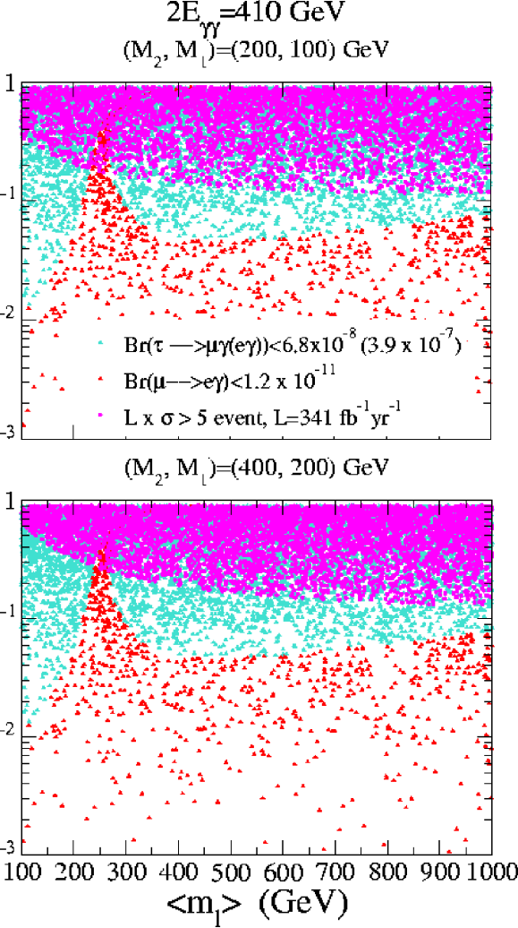
Figure 10: Scatter plot in the plane ($\delta_{LL},\widetilde{m}$) of: (a) the experimental bounds from $\mu\to e\gamma$ and $\tau\to\mu\gamma$ (allowed regions with circular dots); (b) regions where the signal can give at least five events at year for two sets of gaugino masses. The energy is $\sqrt{s_{\gamma\gamma}}=410$ GeV and the luminosity $L=341$ fb^-1 yr^-1.

In Figures 9, 10 we show scatter plots where the average lepton masses and the relative mass splitting $\delta_{LL}=\Delta m^{2}/\widetilde{m}^{2}$ are varied freely, for fixed values of gaugino masses. All the parameter space [the $(\widetilde{m},\delta_{LL})$ plane] is covered by the clear triangle-up shaped points (turquoise in color) that satisfy the bounds $\Gamma(\tau\to\gamma\mu,(e))<6.8\times 10^{-8}\;3.9\times 3.9\times 10^{-7}$ while the black triangle-up shaped points (red in color), that satisfy $\Gamma(\mu\to e\gamma)<1.2\times 10^{-11}$ cover a more restricted part. The grey circle shaped points (magenta in color) are determined imposing the condition that the total cross section multiplied by the luminosity gives more than five events per year. We can note two things: the signal’s points overlap with the “$\mu,e$” region only on the tail of the red region extending to higher values of $\delta_{LL}$. This tail is due to some peculiar cancellation between diagrams, as discussed in Ref. hisa2 , thus we can say that this possible final state is almost excluded. The $\mu,\tau$ and the $e,\tau$ final state are not excluded but they generally require a high-mass splitting $\delta_{LL}>10^{-1}$.

From the point of view of the supersymmetric seesaw mechanism described in Section II, these values can be realized in nature only under some restricted conditions pascoli : the matrix $Y_{\nu}$ from the seesaw mechanism neutrino masses and mixing is ambiguous up to a complex, orthogonal matrix $R$ casas . Usually this matrix is taken to be real or identical to the unit matrix. In the case of a quasi-degenerate neutrino mass spectrum, $R$ being complex allows for values of $\Delta m^{2}$ larger by 5-8 orders of magnitude relative to the case of $R$ being real or the unit matrix cannoni .

V Standard Model background

Production of charged leptons will be copious in $\gamma\gamma$ collisions, and the SM provides several processes that can mimic $e\tau$, $\mu\tau$ final states. Let us see how to reduce the most important contributions that are :

$$(a)\;\;\gamma\gamma\to\tau^{-}\tau^{+}\to\tau^{-}\nu_{e}\bar{\nu}_{\tau}e^{+}$$ (26)

$$(b)\;\;\gamma\gamma\to{W^{-}}^{*}{{W}^{+}}^{*}\to\tau^{-}{\bar{\nu}}_{\tau}\,{e^{+}}{{\nu}}_{e}$$ (27)

$$(c)\;\;\gamma\gamma\to e^{+}e^{-}\tau^{+}\tau^{-}$$ (28)

with similar processes for the production of $\mu\tau$ pairs. As we have seen, the $e\mu$ final state, which is the easiest to reconstruct from the experimental point of view, is almost completely excluded by the strong bounds from the non observation of the radiative decay $\mu\to e\gamma$. Thus we are bound to consider signals with a tau in the final state. Taus can, in principle, be reconstructed looking at the associated leptonic decay $\tau\to\ell\nu\bar{\nu}$ and at the hadronic decay $\tau\to\pi^{\pm}\pi^{0}$. The cross sections of processes in Eqs. (26-27) depend on initial photon polarizations, while the reaction in Eq. (28) is almost insensitive to photon helicities. We use the program COMPHEP comphep , and the CB spectra with $z>0.8z_{max}$. In Table 1 we give the values of the cross sections after the application of kinematical cuts (contributions of the charge-conjugate processes are also included).

Table 1: Total cross section without and with cuts described in the text for the background processes Eqs. (26-28).

2$E_{0}$ (GeV)		$\gamma\gamma\to\tau\tau\to\tau e\nu\bar{\nu}$	$\gamma\gamma\to WW\to e\tau\nu\bar{\nu}$	$\gamma\gamma\to\tau\tau ee$
200	$\sigma$	0.58 fb	2.3$\times 10^{-1}$	36.7 pb
	$\sigma_{cut}$	1.49$\times 10^{-6}$ fb	//	4.4$\times 10^{-2}$ fb
300	$\sigma$	3.1 fb	0.48 pb	38.9 pb
	$\sigma_{cut}$	16.3$\times 10^{-6}$ fb	//	3.7$\times 10^{-2}$ fb
400	$\sigma$	4.9 fb	0.69 pb	39.5 pb
	$\sigma_{cut}$	3.9$\times 10^{-4}$ fb	$2.1\times 10^{-2}$ fb	2.9$\times 10^{-2}$ fb
500	$\sigma$	6.1 fb	0.77 pb	39.9 pb
	$\sigma_{cut}$	9.7$\times 10^{-4}$ fb	$1\times 10^{-1}$ fb	2.4$\times 10^{-2}$ fb

Tau pair production, $W$ gauge bosons pair production and four charged fermion production are known to have very large cross sections, at the level of hundreds of picobarn at the CM energy of ILC, orders of magnitude larger than the signal in the most favourable regions of the parameter space. However the signal is characterized by two back-to-back leptons with the energy of the beams without missing transverse momentum and energy. These characteristics provide also indications on the necessary kinematical cuts to be applied to the background processes.

The helicity amplitudes which dominate the signal $(+,-)$ and $(-,+)$, are peaked along the collision axis. Most of the background is also concentrated in this region. So we apply the angular cut $|\cos(\theta)|<0.9$ ($\theta<25.8^{\circ}$) both to the signal and to the background. We also impose the back-to-back condition on the background processes, requiring $180^{\circ}-\theta_{\ell\ell^{\prime}}<5^{\circ}$. Using in addition the condition that one of the event hemisphere should consist of a single muon or electron with energy close to $E_{\gamma}$, final leptons are required to have energy at least $85\%$ of the maximum photon energy $E^{\gamma}_{max}=y_{max}E_{0}$.

As can be seen from Table 1, after these cuts are applied, process $(a)$ is suppressed because tau pairs are almost produced along the collision axis, and process $(b)$ is completely excluded, at least for low energies, because the leptons from the decay of $W$ are less energetic and cannot survive to the energy cut. Instead, due to the well known rapid growth of the $\gamma\gamma\to WW$ cross section above threshold, at $400$ and $500$ GeV CMF energy, these cuts are not enough to suppress the background, giving cross sections of $2.1\times 10^{-2}$ fb and $10^{-1}$ fb respectively. However with a cut on the transverse momentum of the electron $p_{T}^{e}>15$ GeV the cross section, at $\sqrt{s_{ee}}=500$ GeV, is reduced to $2.1\times 10^{-2}$ fb, while for $p_{T}^{e}>20$ GeV, the contribution is eliminated.

Reaction $(c)$ turns out to provide the most dangerous background. In this case the results were obtained with a MonteCarlo code developed by some of the authors carimalo , which uses some compact analytical expressions for the diagrams with the exchange of space-like photons. The configuration that mimics the signal arises if one $e\tau$ pair is emitted at small angle with respect the collision axis and is not detected (we require $\theta_{\ell}^{untagged}<25.8^{\circ}$), while the other pair is tagged. This configuration is determined by multi-peripheral diagrams as a consequence of $t$-channel poles at small angles. The detected pair presents characteristics very similar to those of the signal, and though the cross section is effectively reduced by orders of magnitudes, it is still at the level of $10^{-2}$ fb, thus remaining competitive with the signal cross section. However, at a final step, this background can be estimated from the data by requiring instead that the detected tau and electron be of the same charge, and eventually subtracted. After the cuts discussed above this is the only significant background contribution which remains. We consider the statistical significance

$$SS=\frac{{\cal L}\sigma_{cut}^{S}}{\sqrt{{\cal L}\sigma_{cut}^{BG}}}$$

and requiring $SS\geq 3$ we obtain $\sigma_{cut}^{S}>5.4\times 10^{-2}$ fb at $\sqrt{s_{ee}}=200$ GeV and $\sigma_{cut}^{S}>2.5\times 10^{-2}$ fb at $\sqrt{s_{ee}}=500$ GeV, using the simulated annual luminosity for TESLA. By inspection of Fig. 7 and Fig. 8 it is seen that this condition is in both cases satisfied if $\delta_{LL}\gtrsim 10^{-1}$ with the values of the other SUSY parameters as specified previously. This region of the parameter space is allowed for the $e\tau$, $\mu\tau$ channels as can be seen in Fig. 9 and Fig. 10.

VI Summary and conclusions

We have studied the lepton flavor violating reactions ${\gamma\gamma\to\ell\ell^{\prime}}$ (${\ell,\ell^{\prime}=e,\mu,\tau}$, $\ell\neq\ell^{\prime}$) which arise at the one loop order of perturbation theory and which will be of interest for the $\gamma\gamma$ option of the future ILC. The LFV mechanism is provided by low energy R-conserving supersymmetry with non diagonal slepton mass matrices. The origin of the non diagonal entries of the charged slepton mass matrices can be ascribed to a SUSY seesaw mechanism with mSugra boundary conditions, a theoretical scenario that has attracted much attention in the literature in recent years. We have studied the signal in a model independent way in order to pin down regions of the SUSY parameter space, the ($\widetilde{m}_{\ell},\delta_{LL}$) plane, allowed by the present experimental limits.

We have shown that in the range 200-500 GeV for the center of mass energy of the basic electron collider that produces photon beams, the cross section of the signal is $\sigma(\gamma\gamma\to\ell\ell^{\prime})={\cal O}(10^{-1}\,-\,10^{-2})$ fb for sparticle masses in the range $90-200$ GeV that correspond to a light SUSY spectrum somehow hinted to by fits on standard model parameters and SUSY benchmark points. Observation at a PC of $\gamma\gamma\to e\tau$, $(\mu\tau)$ is not excluded by present bounds on the radiative lepton decays $\tau\to e\gamma$, $\tau\to\mu\gamma$ which do not constrain the parameter space strongly enough, nonetheless a relative mass splitting $\delta_{LL}={\Delta m^{2}}/{\widetilde{m}_{\ell}^{2}}$ at least of order $10^{-1}$ is required, a value that can be obtained in the SUSY seesaw framework but only within some particular model. The $e\mu$ final state is almost excluded because of the stronger constraint provided by the upper bound on the branching ratio given by the non observation of $\mu\to e\gamma$ which is four orders of magnitude smaller than those provided by the non observation of $\tau\to e\gamma$, $\tau\to\mu\gamma$.

The nice signal’s feature of having two back-to-back high energy leptons in the final state can be somewhat altered by the non-monochromaticity of the photon beams produced via Compton backscattering. So we have restricted the numerical analysis to the high-energy part of the luminosity spectrum of the photon collider: on the other hand this part corresponds to collisions of almost monochromatic and polarized photons, with an integrated luminosity close to that of the basic lepton collider. Under the very same conditions we have studied the standard model background and shown that with suitable cuts it can be taken at the level of $\sigma_{back}\approx{\cal O}(10^{-2})$ fb. The process $\gamma\gamma\to ee(\mu\mu)\tau\tau$ presents a configuration with an undetected $e\tau$ pair emitted at small angle along the collision axis and with the detected pair of high energy leptons almost back-to-back, has a potentially large cross section which can easily mimic the LFV signal. We have considered the signal statistical significance and found that one can obtain $SS\gtrsim 3$ provided that $\delta_{LL}\gtrsim 10^{-1}$.

Appendix A Helicity Amplitudes

In this appendix we present explicit expressions for the helicity amplitudes of the diagrams depicted in Fig. 1.

(a)

Penguin diagrams

These are the diagrams depicted in part (a) of Fig. 1. We have two types of contributions: the chargino-sneutrino loop and the slepton-neutralino loop:

1. Chargino-sneutrino

   $${\cal M}^{\lambda\lambda^{\prime}}_{i}=+i\frac{e^{2}(O_{\widetilde{\nu}}^{\widetilde{W}})^{2}}{16\pi^{2}}\,X^{\lambda\lambda^{\prime}}_{i}\qquad(i=1,2)$$ (29)

   $$X^{++}_{1} = +\sin\theta^{*}\,\left[(C_{0}M_{\widetilde{W}}^{2}-2C_{00})+s(C_{1}+C_{11}+C_{12})\right]$$

   $$X^{+-}_{1} = +\sin\theta^{*}\,\left(C_{0}M_{\widetilde{W}}^{2}-2C_{00}\right)\left[\frac{1-\cos\theta^{*}}{1+\cos\theta^{*}}\right]$$

   $$X^{-+}_{1} = -\sin\theta^{*}\,\left(C_{0}M_{\widetilde{W}}^{2}-2C_{00}\right)$$

   $$X^{--}_{1} = +\sin\theta^{*}\,\left(C_{0}M_{\widetilde{W}}^{2}-2C_{00}\right)$$

   $$X^{++}_{2} = +\sin\theta^{*}\,(C_{0}M_{\widetilde{W}}^{2}-2C_{00})$$

   $$X^{+-}_{2} = +\sin\theta^{*}\,\left(C_{0}M_{\widetilde{W}}^{2}-2C_{00}\right)\left[\frac{1-\cos\theta^{*}}{1+\cos\theta^{*}}\right]$$

   $$X^{-+}_{2} = -\sin\theta^{*}\,\left(C_{0}M_{\widetilde{W}}^{2}-2C_{00}\right)$$

   $$X^{--}_{2} = +\sin\theta^{*}\,\left[\left(C_{0}M_{\widetilde{W}}^{2}-2C_{00}\right)+s(C_{2}+C_{12}+C_{22})\right]$$

   In the above expressions the three-point form factors ($C^{\prime}s$) are to be evaluated with the following arguments:

   $$C_{...}=C_{...}(t,0,0,m_{\widetilde{\chi}_{j}^{0}}^{2},m_{\widetilde{\ell}}^{2},m_{\widetilde{\ell}}^{2})\quad(i=1)$$

   $$C_{...}=C_{...}(0,0,t,m_{\widetilde{\chi}_{j}^{0}}^{2},m_{\widetilde{\ell}}^{2},m_{\widetilde{\ell}}^{2})\quad(i=2)$$

2. Slepton-neutralino

   $${\cal M}^{\lambda\lambda^{\prime}}_{i}=+i\frac{e^{2}}{8\pi^{2}}\,\sum_{j}(O^{\widetilde{\ell}}_{\widetilde{\chi}_{j}^{0}})^{2}X^{\lambda\lambda^{\prime}}_{i}\qquad(i=1,2)$$ (30)

   $$X^{++}_{1} = +\sin\theta^{*}\,\left[+C_{00}+\frac{s}{4}(1-\cos\theta^{*})(C_{1}+C_{11}+C_{12})\right]$$

   $$X^{+-}_{1} = +\sin\theta^{*}\,\left\{+C_{00}\left[\frac{1-\cos\theta^{*}}{1+\cos\theta^{*}}\right]-\frac{s}{4}(1-\cos\theta^{*})(C_{1}+C_{11}+C_{12})\right\}$$

   $$X^{-+}_{1} = +\sin\theta^{*}\,\left[-C_{00}-\frac{s}{4}(1+\cos\theta^{*})(C_{1}+C_{11}+C_{12})\right]$$

   $$X^{--}_{1} = +\sin\theta^{*}\,\left[+C_{00}-\frac{s}{4}(1+\cos\theta^{*})(C_{1}+C_{11}+C_{12})\right]$$

   $$X^{++}_{1} = +\sin\theta^{*}\,\left[+C_{00}-\frac{s}{4}(1+\cos\theta^{*})(C_{2}+C_{12}+C_{22})\right]$$

   $$X^{+-}_{1} = +\sin\theta^{*}\,\left\{+C_{00}\left[\frac{1-\cos\theta^{*}}{1+\cos\theta^{*}}\right]-\frac{s}{4}(1-\cos\theta^{*})(C_{2}+C_{12}+C_{22})\right\}$$

   $$X^{-+}_{1} = +\sin\theta^{*}\,\left[-C_{00}+\frac{s}{4}(1+\cos\theta^{*})(C_{2}+C_{12}+C_{22})\right]$$

   $$X^{--}_{1} = +\sin\theta^{*}\,\left[+C_{00}+\frac{s}{4}(1-\cos\theta^{*})(C_{2}+C_{12}+C_{22})\right]$$

   In the above expressions the three-point form factors ($C^{\prime}s$) are to be evaluated with the following arguments:

   $$C_{...}=C_{...}(t,0,0,m_{\widetilde{\nu}}^{2},M_{\widetilde{W}}^{2},M_{\widetilde{W}}^{2})\quad(i=1)$$

   $$C_{...}=C_{...}(0,0,t,m_{\widetilde{\nu}}^{2},M_{\widetilde{W}}^{2},M_{\widetilde{W}}^{2})\quad(i=2)$$

(b)

Self-energy diagrams

1. external leg corrections

   • slepton-neutralino

     $$({\cal M}_{3a}+{\cal M}_{4a})^{\lambda\lambda^{\prime}}=-i\frac{e^{2}}{16\pi^{2}}\sum_{j}O_{\widetilde{\chi}_{j}^{0}}^{\ell^{\prime}}O_{\widetilde{\chi}_{j}^{0}}^{\ell}\,2\,\left[B_{0}+B_{1}\right](0,m_{\widetilde{\ell}}^{2},m_{\widetilde{\chi}^{0}_{j}}^{2})\,X^{\lambda\lambda^{\prime}}\,$$ (31)

   • chargino-sneutrino

     $$({\cal M}_{3b}+{\cal M}_{4b})^{\lambda\lambda^{\prime}}=-i\frac{e^{2}}{16\pi^{2}}(O_{\widetilde{\nu}}^{\widetilde{W}})^{2}\,2\,\left[B_{0}+B_{1}\right](0,m_{\widetilde{\nu}}^{2},m_{\widetilde{W}}^{2})X^{\lambda\lambda^{\prime}}\,$$ (32)

2. t-channel correction ${\cal M}_{5}={\cal M}_{5a}+{\cal M}_{5b}$

   • slepton-neutralino

     $${\cal M}_{5a}^{\lambda\lambda^{\prime}}=-i\frac{e^{2}}{16\pi^{2}}\sum_{j}O_{\widetilde{\chi}_{j}^{0}}^{\ell^{\prime}}O_{\widetilde{\chi}_{j}^{0}}^{\ell}\left[B_{0}(t,m_{\widetilde{\ell}}^{2},m_{\widetilde{\chi}^{0}_{j}}^{2})+B_{1}(t,m_{\widetilde{\ell}}^{2},m_{\widetilde{\chi}^{0}_{j}}^{2})\right]X^{\lambda\lambda^{\prime}}\,$$ (33)

   • chargino-sneutrino

     $${\cal M}_{5b}^{\lambda\lambda^{\prime}}=-i\frac{e^{2}}{16\pi^{2}}(O_{\widetilde{\nu}}^{\widetilde{W}})^{2}\,\left[B_{0}(t,m_{\widetilde{\nu}}^{2},m_{\widetilde{W}}^{2})+B_{1}(t,m_{\widetilde{\nu}}^{2},m_{\widetilde{W}}^{2})\right]X^{\lambda\lambda^{\prime}}\,$$ (34)

   The helicity factor is the same in this case:

   $$X^{\lambda\lambda^{\prime}}=\frac{\sin\theta^{*}}{1+\cos\theta^{*}}\,\left[\frac{1+\lambda\lambda^{\prime}+\lambda-\lambda^{\prime}}{2}+\lambda\lambda^{\prime}\cos\theta^{*}\right]\,$$

   $$X^{++} = +\sin\theta^{*}$$

   $$X^{+-} = +\sin\theta^{*}\frac{1-\cos\theta^{*}}{1+\cos\theta*}$$

   $$X^{-+} = -\sin\theta^{*}$$

   $$X^{--} = +\sin\theta^{*}$$

(c)

Sea-Gull and Box diagrams

These are the diagrams depicted in part (c) of Fig. 1.

• (Seagull) The seagull type diagram has only a contribution from a slepton-neutralino loop (${\cal M}_{6}$).

  $${\cal M}^{\lambda\lambda^{\prime}}_{6}=0$$

• (Scalar Box)

  This is the slepton neutralino box diagram in part(c) of Fig. 1 (${\cal M}_{7}$).

  $${\cal M}^{\lambda\lambda^{\prime}}_{7} = +i\frac{e^{2}}{16\pi^{2}}\sum_{j}(O_{\widetilde{\chi}_{j}^{0}}^{\widetilde{\ell}})^{2}\,4\left(\frac{s}{2}\sin\theta^{*}\right)\,\left[\frac{1+\lambda\lambda^{\prime}}{2}D_{002}\right.$$ (35)

  $$-\left(\frac{\lambda-\lambda^{\prime}}{2}+\lambda\lambda^{\prime}\cos\theta^{*}\right)(D_{00}+D_{001}+D_{002}+D_{003})$$

  $$-\frac{s}{8}\lambda\lambda^{\prime}\sin^{2}\theta^{*}\left(D_{112}+2D_{122}+2D_{123}+D_{222}+2D_{223}+D_{233}\right.$$

  $$\left.\left.+D_{2}+2(D_{12}+D_{22}D_{23}\right)\phantom{\frac{1}{2}}\right]$$

  The $D$ form factors appearing in the above formula for the scalar box diagram are to be evaluated with the following arguments:

  $$D_{...}=D_{...}(0,0,0,0,t,s,m_{\chi_{j}^{0}}^{2},m_{\widetilde{\ell}}^{2},m_{\widetilde{\ell}}^{2},m_{\widetilde{\ell}}^{2})$$

• Chargino-sneutrino loop

  This is the box diagram involving fermions depicted as (${\cal M}_{8}$) in part(c) of Fig. 1.

  $${\cal M}_{8}^{\lambda\lambda^{\prime}}=-i\frac{e^{2}}{16\pi^{2}}\,(O_{\widetilde{\nu}}^{\widetilde{W}})^{2}\,\left[\sum_{i}\langle i\rangle^{\lambda\lambda^{\prime}}D_{i}+\sum_{ij}\langle ij\rangle^{\lambda\lambda^{\prime}}D_{ij}+\sum_{ijk}\langle ijk\rangle^{\lambda\lambda^{\prime}}D_{ijk}\right]$$ (36)

  The various (non-zero) coefficients multilplying the four-point loop form factors ($D_{i},D_{ij},D_{ijk}$) are given below:

  $$\langle 0\rangle^{\lambda\lambda^{\prime}} = -M_{\widetilde{W}}^{2}\,\frac{s}{4}\,\sin\theta^{*}\left(1+\lambda\lambda^{\prime}+\lambda-\lambda^{\prime}+2\lambda\lambda^{\prime}\cos\theta^{*}\right)$$

  $$\langle 1\rangle^{\lambda\lambda^{\prime}} = +M_{\widetilde{W}}^{2}\,\frac{s}{2}\,\lambda^{\prime}\sin\theta^{*}\left(1-\lambda\cos\theta^{*}\right)$$

  $$\langle 2\rangle^{\lambda\lambda^{\prime}} = +M_{\widetilde{W}}^{2}\,\frac{s}{4}\,\sin\theta^{*}\left(1+\lambda\lambda^{\prime}-(\lambda-\lambda^{\prime})-2\lambda\lambda^{\prime}\cos\theta^{*}\right)$$

  $$\langle 3\rangle^{\lambda\lambda^{\prime}} = -M_{\widetilde{W}}^{2}\,\frac{s}{2}\,\lambda\sin\theta^{*}\left(1+\lambda^{\prime}\cos\theta^{*}\right)$$

  $$\langle 00\rangle^{\lambda\lambda^{\prime}} = +\frac{s}{2}\,\sin\theta^{*}\left[1+\lambda\lambda^{\prime}+(\lambda-\lambda^{\prime})+2\lambda\lambda^{\prime}\cos\theta^{*}\right]$$

  $$\langle 12\rangle^{\lambda\lambda^{\prime}} = +\frac{s^{2}}{4}\,\sin\theta^{*}\,\lambda^{\prime}(1-\lambda)(1+\cos\theta^{*})$$

  $$\langle 13\rangle^{\lambda\lambda^{\prime}} = -\frac{s^{2}}{4}\,\sin\theta^{*}\left[1+\lambda\lambda^{\prime}+(\lambda-\lambda^{\prime})+2\lambda\lambda^{\prime}\cos\theta^{*}\right]$$

  $$\langle 22\rangle^{\lambda\lambda^{\prime}} = -\frac{s^{2}}{8}\,(\lambda-\lambda^{\prime})(1-\lambda)\,\sin\theta^{*}(1+\cos\theta^{*})$$

  $$\langle 23\rangle^{\lambda\lambda^{\prime}} = -\frac{s^{2}}{4}\,\lambda(1+\lambda^{\prime})\,\sin\theta^{*}\,(1+\cos\theta^{*})$$

  $$\langle 001\rangle^{\lambda\lambda^{\prime}} = -s\sin\theta^{*}[\lambda+\lambda^{\prime}+\lambda^{\prime}(1-\lambda\cos\theta^{*})]$$

  $$\langle 002\rangle^{\lambda\lambda^{\prime}} = (\frac{s}{2}\sin\theta^{*})[-(1+\lambda\lambda^{\prime})+\lambda(1+\lambda^{\prime}\cos\theta^{*})-\lambda^{\prime}(1-\lambda\cos\theta^{*})]$$

  $$\langle 003\rangle^{\lambda\lambda^{\prime}} = +{s}\sin\theta^{*}\,[\lambda(1+\lambda^{\prime}\cos\theta^{*})+\lambda+\lambda^{\prime}]$$

  $$\langle 112\rangle^{\lambda\lambda^{\prime}} = +\frac{s^{2}}{4}\,\lambda^{\prime}(1-\lambda)\sin\theta^{*}(1+\cos\theta^{*})$$

  $$\langle 113\rangle^{\lambda\lambda^{\prime}} = +\frac{s^{2}}{2}\,\lambda^{\prime}\sin\theta^{*}(1-\lambda\cos\theta^{*})$$

  $$\langle 133\rangle^{\lambda\lambda^{\prime}} = -\frac{s^{2}}{2}\,\lambda\sin\theta^{*}(1+\lambda^{\prime}\cos\theta^{*})$$

  $$\langle 122\rangle^{\lambda\lambda^{\prime}} = -\frac{s^{2}}{8}\,(3\lambda^{\prime}-\lambda)(1-\lambda)\sin\theta^{*}(1+\cos\theta^{*})$$

  $$\langle 123\rangle^{\lambda\lambda^{\prime}} = +\frac{s^{2}}{2}\sin\theta^{*}\,\left[\lambda^{\prime}(1-\lambda\cos\theta^{*})-\frac{1}{2}(1+\lambda\lambda^{\prime}+\lambda+\lambda^{\prime})\right]$$

  $$\langle 132\rangle^{\lambda\lambda^{\prime}} = \delta_{\lambda+}\,\frac{s^{2}}{2}\,\sin\theta^{*}\,(1+\cos\theta^{*})$$

  $$\langle 222\rangle^{\lambda\lambda^{\prime}} = -\frac{s^{2}}{8}\,(\lambda-\lambda^{\prime})(1-\lambda)\sin\theta^{*}(1+\cos\theta^{*})$$

  $$\langle 223\rangle^{\lambda\lambda^{\prime}} = -\frac{s^{2}}{8}\lambda(1+\lambda^{\prime})(3-\lambda)\,\sin\theta^{*}(1+\cos\theta^{*})$$

  $$\langle 233\rangle^{\lambda\lambda^{\prime}} = -\frac{s^{2}}{4}\,\lambda(1+\lambda^{\prime})\,\sin\theta^{*}\,(1+\cos\theta^{*})$$

The $D$ form factors appearing in the above formula for the chargino sneutrino box diagram are to be evaluated with the following arguments:

$$D_{...}=D_{...}(0,0,0,0,t,s,m_{\widetilde{\nu}}^{2},m_{\widetilde{W}}^{2},m_{\widetilde{W}}^{2},m_{\widetilde{W}}^{2})$$

A diagram with a LFV and a LFC scalar line, for example, is described by the propagators of Eq. (7) and Eq. (8), so that the loop coefficients in the amplitudes are a sum of four integrals, while in the diagrams with only a LFV line, are a sum of two. The scalar two point function $B_{0}$ and the tensor coefficients $B_{1}$, $C_{00}$ that appear in the electroweak penguins are ultra-violet divergent, but the amplitudes are finite due the ortogonality of the slepton mixing matrix. The rule for obtaining the helicity amplitudes for the exchanged diagrams from those of the direct diagrams:

$${\cal M}^{\lambda\lambda^{\prime}}_{exch.}(\sin\theta^{*},\cos\theta^{*})={\cal M}^{\lambda^{\prime}\lambda}_{direct}(-\sin\theta^{*},-\cos\theta^{*})$$ (37)

The loop form factors are exchanged accordingly to the same rule: ($\cos\theta^{*}\to-\cos\theta^{*}$, and $\sin\theta^{*}\to-\sin\theta^{*}$).