Effects of the CP Odd Dipole Operators on Gluino Production at Hadron Colliders

Abstract

We present the cross sections for the hadroproduction of gluinos by taking into account the CP odd dipole operators in supersymmetric QCD. The dependence of the cross sections on these operators is analyzed for the hadron colliders the Tevatron ($\sqrt{S}$=1.8 TeV) and the Cern LHC ($\sqrt{S}$=14 TeV). The enhancement of the hadronic cross section is obviously mass dependent and for a 500 GeV gluino, is up to 16 % (over 73 pb) at the LHC while it is 8 % (over 0.63 fb) at the Tevatron.

I Introduction

Supersymmetric QCD (SUSY-QCD) is based on the colored particles of the Minimal Supersymmetric Standard Model (MSSM) HG ; HP spectrum; quarks, gluons and their superpartners squarks and gluinos. Since supersymmetry is a broken one rather than an exact symmetry, the masses of the superparticles extremely exceed the masses of their SM partners LMT . Upper bound limits of $\mathcal{O}$(1 TeV) are set to these masses for the sake of the solution of the hierarchy problem. In most of the analysis the scalar partners of the five light quarks are assumed mass degenerate WRMZ .

Searching for supersymmetric particles will be one of the main goals of the future experimental program of high energy physics. The particles in the strong interaction sector can be searched for most efficiently at hadron colliders. As they are presently searched at the Tevatron ($\sqrt{s}$= 1.8 TeV) the Large Hadron Collider (LHC) with center of mass energy of $\sqrt{s}$= 14 TeV will in a sense be a gluino factory.

At the fundamental level SUSY receives some additional effects from the existent particles predicted by high energy models so called GUT or String Theory. As these effect are quite general we consider them in gluino pair production. At this level we know the interaction vertices in supersymmetric QCD. After the prediction of Kane and Leville KL for the tree level hadronic production of gluinos several improvements for this process have been performed WRMZ . The production of gluino pairs in electron-positron annihilation is analyzed in ref 4. In the present analysis we reconsider the productions of gluino pairs in hadron-hadron collisions and generalize to include the CP odd terms to investigate the effects of these CP violating operators in these processes. We assumed an updated range of 300-500 GeV for the gluino masses.

II Gluino Production with the CP Violating Terms

The dominant contributions to the production cross sections of gluino pairs in $pp$ or $p\bar{p}$ collisions come from the subprocesses $q\bar{q}\rightarrow\tilde{g}\tilde{g}$ and $gg\rightarrow\tilde{g}\tilde{g}$. The relevant Feynman diagrams are displayed in Figures 1 and 2 and the differential cross sections are calculated in the Appendix. In the first subprocess $q\bar{q}\rightarrow\tilde{g}\tilde{g}$, in principle $\hat{t}$ and $\hat{u}$-channel squark exchanges have also contributions in addition to the annihilation s channel gluion exchange. But these contributions are almost always negligible since squarks of first and second generations must be nearly degenerate and they are heavy to satisfy the Electric Dipole Moment bounds. Therefore we will consider only the s-channel via gluon exchange for the reaction $q\bar{q}\rightarrow\tilde{g}\tilde{g}$. In calculations of the differential cross sections we use the standard structure of the effective CP-odd lagrangian including the Weinberg operator and color EDMs of quarks DOKM ; DMA ; AP and the interaction lagrangian of the gluinos with the gauge field gluons HG to obtain the following three interaction vertices;

i) Quark-quark-gluon

ii) Gluon-gluino-gluino

iii) Three gluon

where $g_{s}$ is the strong coupling constant, $q$ is the momentum carried by the mediator, $d_{q}$ and $\tilde{d}_{g}$ are effective color EDMs couplings of quarks and gluinos respectively. $\Lambda$ denotes the scale up to which the effective theory is assumed to hold. $C^{\mu\nu\rho}(p_{1},p_{2},q)$ is the standard three gluon vertex with all momenta incoming $C^{\mu\nu\rho}(p_{1},p_{2},q)=g^{\mu\nu}(p_{1}-p_{2})^{\rho}+g^{\nu\rho}(p_{2}-q)^{\mu}+g^{\mu\rho}(q-p_{1})^{\nu}$. $C_{W}$ is the coefficient of the Weinberg operator and the term with this coefficient is the result of a straightforward calculation of the dimension-6 Weinberg operator SW :

$$\mathcal{O}_{W}=-\frac{C_{W}}{6}f_{abc}\epsilon^{\mu\lambda\nu\rho}G_{a}^{\mu\lambda}G^{b}_{\nu\sigma}G^{c}_{\rho\sigma}$$ (1)

where $G_{a}^{\mu\nu}$ is gluon field strength tensor.

The differential cross sections are presented in the Appendix. Integrating them over $\hat{t}$ leads to the total partonic cross sections:

$$\hat{\sigma}_{q}(q_{i}\bar{q}_{i}\rightarrow\tilde{g}\tilde{g}) = (\frac{1}{72\pi\hat{s}^{4}})[J(d^{2}{d_{1}}^{2}J^{2}\hat{s}^{2}-g_{s}^{2}\hat{s}((d^{2}+{d_{1}}^{2})J^{2}-12d^{2}m^{2}\hat{s}$$ (2)

$$+3(d^{2}+{d_{1}}^{2})\hat{s}^{2})+g_{s}^{4}(J^{2}+3\hat{s}(4m^{2}+\hat{s})))]$$

where $\hat{s}=x_{1}x_{2}S$ is the partonic CM energy, $J=s\beta$, $\beta=\sqrt{1-\frac{4m^{2}}{\hat{s}}}$ being gluino velocity in the partonic center of mass system, $m$ denotes mass of the produced gluinos, and $d_{1}=d_{q}/2\Lambda$, $d=d_{\tilde{g}}/4\Lambda$. In obtaining Eq.1 only the s-channel of Fig.1 was considered.

For the second subprocess $gg\rightarrow\tilde{g}\tilde{g}$ contributions of all the three diagrams in Fig.2 are considered, and the integrated cross section in this case is obtained as

$$\hat{\sigma}(gg\rightarrow\tilde{g}\tilde{g}) = \frac{1}{2}\frac{1}{512\pi\hat{s}^{4}(J^{2}-\hat{s}^{2})}[3(J(d^{4}\hat{s}^{2}(-5J^{4}+6912m^{8}+3354m^{4}\hat{s}^{2}-480m^{2}\hat{s}^{3}+9\hat{s}^{4}$$

$$+J^{2}(-3354m^{4}+480m^{2}\hat{s}-4\hat{s}^{2}))-4g_{s}^{4}(J^{4}+2J^{2}\hat{s}(-12m^{2}+7\hat{s})$$

$$-3\hat{s}^{2}(64m^{4}-8m^{2}\hat{s}+5\hat{s}^{2}))-2d^{2}g_{s}^{2}\hat{s}(J^{4}+J^{2}(144m^{4}+210m^{2}\hat{s}-25\hat{s}^{2})$$

$$+6\hat{s}(384m^{6}-56m^{4}\hat{s}-35m^{2}\hat{s}^{2}+4\hat{s}^{3}))$$

$$+12dm(4g_{s}^{2}+d^{2}(20m^{2}-3\hat{s}))\hat{s}^{3}(\hat{s}^{2}-J^{2})w$$

$$+12\hat{s}^{3}(J^{2}-\hat{s}^{2})(d^{2}\hat{s}(-4m^{2}+\hat{s})+2g_{s}^{2}(2m^{2}+\hat{s}))w^{2})$$

$$-12\hat{s}(\hat{s}^{2}-J^{2})(4g_{s}^{4}(-4m^{4}+2m^{2}\hat{s}+\hat{s}^{2})$$

$$+d^{3}m^{4}(d(48m^{4}+316m^{2}\hat{s}+3\hat{s}^{2})+16m\hat{s}^{2}w)$$

$$+2dg_{s}^{2}m(4dm(12m^{4}-12m^{2}\hat{s}+\hat{s}^{2})+\hat{s}^{3}w))\log(\frac{J+\hat{s}}{J-\hat{s}}))]$$

with and $w=C_{W}/6\Lambda^{2}$. Since the gluinos are Majarona fermions the statistical factor of 1/2 is implied to avoid double counting.

The total cross section $pp(p\bar{p})\rightarrow g\tilde{g}X$ is calculated as a function of the hadronic CM energy $S$ and gluino mass $m$, by convoluting the cross sections of subprocesses and parton densities through the factorization theorem

$$\sigma_{tot}(s,m)=\int_{\tau_{0}}^{1}d\tau\int_{\tau}^{1}\frac{dx}{x}\frac{1}{1+\delta_{ij}}\sum_{ij}\left[f_{i}(x)f_{j}(\frac{\tau}{x})+f_{i}(\frac{\tau}{x})f_{j}(x)\right]\hat{\sigma}(m,\hat{s},\hat{u})$$ (4)

where $(i,j)=(g,g)$, $(q_{\alpha},\bar{q}_{\alpha})$, $\alpha=u,d,s$. In performing the calculations we used the Feynman gauge for the internal gluon propagators. We have also used $-g^{\mu\nu}$ for the polarization sum of the external gluons by adding the ghost term. In Tables I-IV we have presented the cross sections for the gluino masses of 300, 400 and 500 GeV to see the $\Lambda$ and mass dependence. The calculated cross sections are not very sensitive to the $\Lambda$ values but drop fast with the increasing mass values. The $gg$ initial state is always dominant at the LHC. At the Tevatron for m=300 GeV the $q\bar{q}$ cross sections are grater than the $gg$ cases, but the situation is reversed for the masses of 400 or 500 GeV.

$\Lambda$ (GeV)	m=300 GeV	m=400 GeV	m=500 GeV
800	0.227689	0.0136852	0.000536575
1000	0.221508	0.0131209	0.000506254
2000	0.2133299	0.0123716	0.000465985
4000	0.211253	0.0121849	0.000455946
6000	0.210874	0.0121503	0.000454088
8000	0.210741	0.0121382	0.000453438

Table 1: The hadronic cross sections in pb for the $q\bar{q}$ initial states at the Tevatron ($\sqrt{s}$= 1.8 TeV)

$\Lambda$ (GeV)	m=300 (GeV)	m=400 (GeV)	m=500 (GeV)
800	0.352658	0.00868101	0.000174379
1000	0.352641	0.0086626	0.000172692
2000	0.353933	0.00873083	0.000174725
4000	0.354495	0.0087646	0.000176001
6000	0.354610	0.00877161	0.000176271
8000	0.354652	0.00877412	0.000176369

Table 2: The hadronic cross sections in pb for the $gg$ initial states at the Tevatron ($\sqrt{s}$= 1.8 TeV)

$\Lambda$ (GeV)	m=300 (GeV)	m=400 (GeV)	m=500 (GeV)
800	25.9082	12.8225	7.37316
1000	24.1935	11.5765	6.43782
2000	22.0388	10.0294	5.28865
4000	21.5236	9.66296	5.01886
6000	21.4292	9.59601	4.96966
8000	21.3963	9.57264	4.9525

Table 3: The hadronic cross sections in pb for the $q\bar{q}$ initial states at the LHC ($\sqrt{s}$= 14 TeV)

$\Lambda$ (GeV)	m=300 (GeV)	m=400 (GeV)	m=500 (GeV)
800	324.288	163.190	91.125
1000	306.743	148.258	78.410
2000	293.053	137.326	69.599
4000	291.167	136.018	68.681
6000	290.884	135.837	68.565
8000	290.791	135.778	68.529

Table 4: The hadronic cross sections in pb for the $gg$ initial states at the LHC ($\sqrt{s}$= 14 TeV)

III Discussion and Conclusion

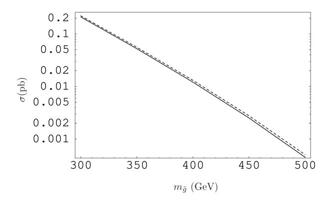
Figure 3: The total cross sections for the $qq$ initial states for the Tevatron with $\Lambda$=1 TeV.

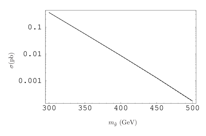
Figure 4: The total cross sections for the $gg$ initial states for the Tevatron with $\Lambda$=1 TeV.

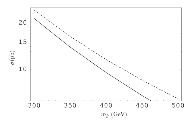
Figure 5: The total cross sections for the $qq$ initial states for the LHC with $\Lambda$=1 TeV.

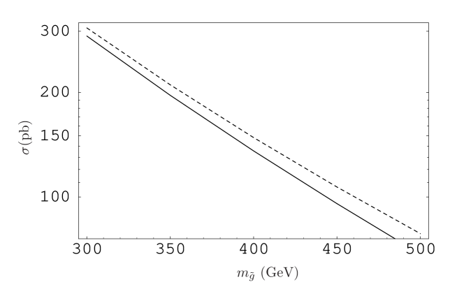
Figure 6: The total cross sections for the $gg$ initial states for the LHC with $\Lambda$=1 TeV.

The results for the $p\bar{p}(pp)\rightarrow\tilde{g}\tilde{g}X$ cross sections are presented in Fig.3 for $q\bar{q}$ annihilation and in Fig.4 for $gg$ fusion at the Tevatron by fixing $\Lambda$=1000 GeV. Similarly the corresponding results are presented in Fig.5 and Fig.6 at the LHC. The solid lines are displayed for $d$=$d_{1}$=$w$=0, without CP violating terms and dotted lines are displayed by taking the contributions of CP-odd terms. For illustrations all effective couplings $d_{q}$, $d_{\tilde{g}}$ and $C_{W}$ are set equal to 1. We used MRST MRST parametrization in convoluting of parton densities. We treated the gluon and light quark flavors as massless. From Fig.4 it is obvious that effects of the CP violating terms in lagrangian are negligible at the Tevatron for the $gg$ fusion. The enhancements in the total hadronic cross sections at this collider for gluinos of masses 300, 400, and 500 GeV are 1.5 %, 4.2 %, and 7.9 % respectively. However the event rates are very low due to the low cross sections; for instance the number of events for 500 GeV gluinos at the Tevatron with an integrated luminosity of 2 $fb^{-1}$ is only 1-2 per year.

At the LHC, the event rates are substantially high; for instance the number of events for 500 GeV gluinos is as high as $10^{7}$ in each LHC detector for a high integrated luminosity of 100 $fb^{-1}$.

In addition to the high event rates at the LHC, CP odd terms give extra contributions, for instance the enhancements in the total hadronic cross sections for 300, 400, and 500 GeV gluinos are 6 %, 10 %, and 16 % respectively. Main contribution to the enhancements comes from the Weinberg term, especially at high mass values. Finally gluon-gluon fusion is always the dominant process in pp collisions such that the LHC can be treated as a gluon-gluon collider, at a first approximation.

Appendix A Color Factors

The generators of SU_c(3) are defined by the commutation relations

$$[T_{a},T_{b}]=if_{abc}T_{c}$$ (5)

The matrices defined as $F_{bc}^{a}=-if_{abc}$ also satisfy similar relations $[F_{a},F_{b}]=if_{abc}F_{c}$ which means that $F_{a}$ form the adjoint representation of SU_c(3). Fundamental identities we have used in this work for the traces of color matrices in the fundamental and adjoint representations are

$$TrT_{a}=0$$

$$Tr(T^{a}T^{b})=\frac{1}{2}\delta_{ab}$$

$$Tr(F_{a}F_{b})=3\delta_{ab}$$

$$Tr(F_{a}F_{b}F_{c})=i\frac{3}{2}f_{abc}$$

$$Tr(F_{a}F_{b}F_{a}F_{c})=\frac{9}{2}\delta_{bc}$$

$$f_{acd}f_{bcd}=3\delta_{ab}$$

$$f_{abc}f_{abc}=24$$ (6)

Because of different color factors, it is convenient to express the square of the matrix element in the form

$$|M(gg\rightarrow\tilde{g}\tilde{g})|^{2} = C_{ss}|M_{s}|^{2}+C_{tt}|M_{t}|^{2}+C_{uu}|M_{u}|^{2}+2C_{st}M_{s}\bar{M}_{t}-2C_{su}M_{s}\bar{M}_{u}$$

$$-2C_{tu}M_{t}\bar{M}_{u}$$

where the obtained values of color factors are

$$C_{ss}=C_{tt}=C_{uu}=72$$

$$C_{st}=C_{su}=-C_{tu}=36$$ (8)

The color factor of $|M(q\bar{q}\rightarrow\tilde{g}\tilde{g})|^{2}$ is obtained to be 12.

Appendix B Differential Cross Sections

The differential cross sections to produce gluino pairs are determined from the Feynman diagrams of Figures 1 and 2 via the subprocesses $q\bar{q}\rightarrow\tilde{g}\tilde{g}$ and $gg\rightarrow\tilde{g}\tilde{g}$ respectively and obtained as

$$\frac{d\hat{\sigma}(q\bar{q}\rightarrow\tilde{g}\tilde{g})}{d\hat{t}} = \frac{1}{12\,\pi\,\hat{s}^{4}}[d^{2}{d_{1}}^{2}{(\hat{t}-\hat{u})}^{2}{(-2m^{2}+\hat{t}+\hat{u})}^{2}$$

$$+2g_{s}^{4}(6m^{4}+\hat{t}^{2}+\hat{u}^{2}-4m^{2}(\hat{t}+\hat{u}))$$

$$-4g_{s}^{2}(2m^{2}-\hat{t}-\hat{u})(({d_{1}}^{2}(m^{2}-\hat{t})(m^{2}-\hat{u}))+d^{2}(m^{4}-\hat{t}\hat{u}))]$$

by considering only s-channel of Fig.1, and

$$\frac{d\hat{\sigma}(gg\rightarrow\tilde{g}\tilde{g})}{d\hat{t}} = \frac{9}{512\pi\hat{s}^{2}}[M_{s}^{2}+M_{t}^{2}+M_{u}^{2}+M_{st}+M_{su}+M_{tu}]$$ (10)

with

$$M_{s}^{2} = \frac{4}{\hat{s}^{2}}[4\,g_{s}^{4}(m^{2}-\hat{t})(m^{2}-\hat{u})-w^{2}d^{2}\,{(-2\,m^{2}+\hat{t}+\hat{u})}^{4}(2\,m^{2}+\hat{t}+\hat{u})$$

$$+g_{s}^{2}(2\,m^{2}-\hat{t}-\hat{u})(d^{2}\,{(\hat{t}-\hat{u})}^{2}+2\,w^{2}(4\,m^{2}-\hat{t}-\hat{u})\,{(-2\,m^{2}+\hat{t}+\hat{u})}^{2})]$$

$$M_{t}^{2} = \frac{-2}{(\hat{t}-m^{2})^{2}}[4\,g_{s}^{4}(m^{4}-\hat{t}\,\hat{u}+m^{2}(3\,\hat{t}+\hat{u}))+2\,g_{s}^{2}\,d^{2}(5\,m^{6}-59\,m^{4}\,\hat{t}+3\,\hat{t}^{3}+m^{2}\,\hat{t}(7\,\hat{t}-4\,\hat{u}))$$

$$+d^{4}\,\hat{t}(4\,m^{6}+67\,m^{4}\,\hat{t}+\hat{t}^{2}(4\,\hat{t}-\hat{u})+m^{2}\,\hat{t}(69\,\hat{t}+\hat{u}))]$$

$$M_{u}^{2} = \frac{-2}{(\hat{u}-m^{2})^{2}}[4\,g_{s}^{4}(m^{4}-\hat{t}\,\hat{u}+m^{2}(\hat{t}+3\,\hat{u}))+2\,g_{s}^{2}\,d^{2}(5\,m^{6}-59\,m^{4}\,\hat{u}+3\,\hat{u}^{3}+m^{2}\,\hat{u}(7\,\hat{u}-4\,\hat{t}))$$

$$+d^{4}\,\hat{u}(4\,m^{6}+67\,m^{4}\,\hat{u}+\hat{u}^{2}(4\,\hat{u}-\hat{t})+m^{2}\,\hat{u}(69\,\hat{u}+\hat{t}))]$$

$$M_{st} = \frac{4}{\hat{s}(\hat{t}-m^{2})}[2\,g_{s}^{4}(m^{4}-2\,m^{2}\,\hat{u}+\hat{t}\,\hat{u})-wd^{3}\,m(m^{4}+4\,m^{2}\,\hat{t}+3\,\hat{t}^{2})\,{(-2\,m^{2}+\hat{t}+\hat{u})}^{2}$$

$$+g_{s}^{2}d(3\,d\,\hat{t}(m^{4}+\hat{t}\,\hat{u}+m^{2}(-3\,\hat{t}+\hat{u}))-m(\hat{t}-\hat{u})\,{(-2\,m^{2}+\hat{t}+\hat{u})}^{2}\,w)]$$

$$M_{su} = \frac{4}{\hat{s}(\hat{u}-m^{2})}[2\,g_{s}^{4}(m^{4}-2\,m^{2}\,\hat{t}+\hat{t}\,\hat{u})-wd^{3}\,m\,{(-2\,m^{2}+\hat{t}+\hat{u})}^{2}(m^{4}+4\,m^{2}\,\hat{u}+3\,\hat{u}^{2})$$

$$+g_{s}^{2}d(3\,d\,\hat{u}(m^{4}+m^{2}(\hat{t}-3\,\hat{u})+\hat{t}\,\hat{u})+wm(\hat{t}-\hat{u})\,{(-2\,m^{2}+\hat{t}+\hat{u})}^{2})]$$

$$M_{tu} = \frac{2}{(\hat{t}-m^{2})(\hat{u}-m^{2})}[4\,g_{s}^{4}\,m^{2}(\hat{s}-4\,m^{2})+d^{4}\,m^{2}(13\,m^{6}-7\,m^{4}(\hat{s}-10\,\hat{u})+2\,\hat{s}\,\hat{u}(\hat{s}+\hat{u})$$

$$-m^{2}\,\hat{u}(39\,\hat{s}+35\,\hat{u}))+d^{2}\,g_{s}^{2}(-140\,m^{6}+\hat{s}\,\hat{u}(\hat{s}+\hat{u})+m^{4}(49\,\hat{s}+88\,\hat{u})$$

$$-m^{2}(\hat{s}^{2}+46\,\hat{s}\,\hat{u}+44\,\hat{u}^{2}))]$$

where $d_{1}=d_{q}/2\Lambda$, $d=d_{\tilde{g}}/4\Lambda$ and $w=C_{W}/6\Lambda^{2}$.

In the special case of $d_{1}$=$d$=$w$=0 we obtain the following result for the differential cross section for the gluino production which agrees with references Harrison:1982yi ; Dawson:1983fw :

$$\frac{d\hat{\sigma}(gg\rightarrow\tilde{g}\tilde{g})}{d\hat{t}} = \frac{9\pi\alpha_{s}^{2}}{4s^{2}}[\frac{2\,\left(m^{2}-t\right)\,\left(m^{2}-u\right)}{s^{2}}-\frac{m^{4}-t\,u+m^{2}\,\left(3\,t+u\right)}{{\left(m^{2}-t\right)}^{2}}-\frac{m^{4}-t\,u+m^{2}\,\left(t+3\,u\right)}{{\left(m^{2}-u\right)}^{2}}$$ (11)

$$+\frac{m^{4}-2\,m^{2}\,t+t\,u}{s\left(u-m^{2}\right)}+\frac{m^{4}-2\,m^{2}\,u+t\,u}{s\left(t-m^{2}\right)}+\frac{m^{2}\,\left(s-4\,m^{2}\right)}{\left(m^{2}-t\right)\,\left(m^{2}-u\right)}]$$

but we should note that the denominators (or numerators) of $s-t$ and $s-u$ terms should be exchanged in Eq.(3.10) of ref Dawson:1983fw and Eq.(3.1) of ref Harrison:1982yi .

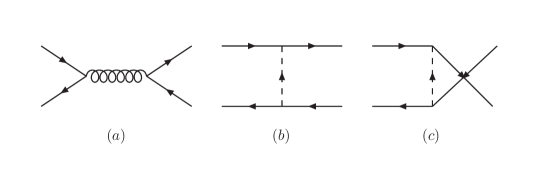
Figure 1: $qq\rightarrow\tilde{g}\tilde{g}$

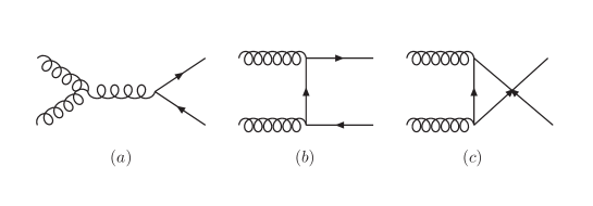
Figure 2: $gg\rightarrow\tilde{g}\tilde{g}$

References

(1)
H. E. Haber and G. L. Kane, Phys. Rep. 117, 75 (1985).
(2)
H. P. Nilles, Phys. Rep. 110, 1 (1984).
(3)
L. Girardello and M. T. Grisaru, Nucl. Phys. B 194, 65
(1982).
(4)
W. Beenakker, R. H pker, M. Spira, P. M. Zerwas, Nucl. Phys. B
492, 51 (1997).
(5)
G. L. Kane, J. P. Leveille, Phys. Lett. B 112, 227
(1982).
(6)
S. Weinberg, Phys. Rev. Lett. 63, 2333 (1989).
(7)
D. A. Demir, O. Lebedev, K. A. Olive, M. Pospelov and A. Ritz,
Nucl. Phys. B 680, 339 (2004).
(8)
D. A. Demir, M. Pospelov and A. Ritz, Phys. Rev. D 67,
015007, (2003).
(9)
A. Pilaftsis, Phys. Rev. D 62, 016007 (2000).
(10)
A. D. Martin, R. G. Roberts, W. J. Stirling and R. S. Thorne,
Eur. Phys. J. C 4, 463 (1998).
(11)
P. R. Harrison and C. H. Llewellyn Smith,
Nucl. Phys. B 213, 223 (1983)
[Erratum-ibid. B 223, 542 (1983)].
(12)
S. Dawson, E. Eichten and C. Quigg,
Phys. Rev. D 31, 1581 (1985).
Figure 1: Figure 2: Figure 3: The total cross sections for the initial states for
the Tevatron with =1 TeV. Figure 4: The total cross sections for the initial states for
the Tevatron with =1 TeV. Figure 5: The total cross sections for the initial states for
the LHC with =1 TeV. Figure 6: The total cross sections for the initial states for
the LHC with =1 TeV.