PITHA 05/10
hep-ph/0508250
August 16, 2005

Heavy-to-light $B$ meson form factors at large recoil energy – spectator-scattering corrections

M. Beneke^a and D. Yang^b
aInstitut für Theoretische Physik E, RWTH Aachen
D–52056 Aachen, Germany
^b Department of Physics, Nagoya University
Nagoya 464-8602, Japan

We complete the investigation of loop corrections to hard spectator-scattering in exclusive $B$ meson to light meson transitions by computing the short-distance coefficient (jet-function) from the hard-collinear scale. Adding together the two coefficients from matching QCD $\to$ SCET_I $\to$ SCET_II, we investigate the size of loop effects on the ratios of heavy-to-light meson form factors at large recoil. We find the corrections from the hard and hard-collinear scales to be of approximately the same size, and significant, but the perturbative expansions appear to be well-behaved. Our calculation provides a non-trivial verification of the factorization arguments. We observe considerable differences between the predictions based on factorization in the heavy-quark limit and current QCD sum rule calculations of the form factors. We also include the hard-collinear correction in the $B\to\pi\pi$ tree amplitudes, and find an enhancement of the colour-suppressed amplitude relative to the colour-allowed amplitude.

1 Introduction

The matrix elements of flavour-changing currents $\bar{q}\hskip 1.42271pt\Gamma_{i}b$ are important strong interaction parameters in low-energy weak-interaction processes. The strong interaction dynamics of semi-leptonic $B$ decays is encoded in these form factors. They are also inputs to the factorization formulae for hadronic two-body $B$ decays [1] and radiative decays [2]. A better understanding of such quantities improves the accuracy of the extraction of the CKM matrix parameters from experimental data, and of searches for new phenomena in flavour-changing processes. Thus efforts are being made to compute the form factors with different methods including QCD lattice simulations [3], light-cone QCD sum rules [4] and quark models [5].

It is also interesting to investigate these form factors in the heavy-quark expansion. It is well-known that all $B\to D^{(*)}$ form factors reduce to a single (Isgur-Wise) function [6] up to calculable short-distance corrections at leading order in this expansion. In this paper we consider transitions of $B$ mesons to light mesons in the large-recoil regime, where the light meson momentum is parametrically of order of the heavy-quark mass. In this regime a similar simplification applies to heavy-to-light form factors [7]: the three (seven) independent $B\to$ pseudoscalar (vector) meson form factors reduce to one (two) function(s) up to corrections that can be calculated in the hard-scattering formalism at leading order in the heavy-quark expansion [8]. The different form factors can therefore be related in a systematic way. The factorization formula that summarizes these statements reads [8]

$$F_{i}^{B\to M}(E)\,=\,C_{i}(E)\,\xi_{a}(E)+\int_{0}^{\infty}\,\frac{d\omega}{\omega}\,\int_{0}^{1}dv\,T_{i}(E;\ln\omega,v)\phi_{B+}(\omega)\phi_{M}(v)$$ (1)

with $E$ the energy of the light meson $M$, $\xi_{a}(E)$ the single non-perturbative form factor (one of the two form factors when $M$ is a vector meson), and $\phi_{X}$ the light-cone distribution amplitudes of the $B$ meson and the light meson. The short-distance coefficients $C_{i}$ and the hard-scattering kernel $T_{i}$ can be calculated in perturbation theory. The heavy-to-light form factors are more complicated than both, the $B\to D^{(*)}$ form factors and light-light meson transition form factors at large momentum transfer. Contrary to the case of $B\to D^{(*)}$, a spectator-scattering correction, the second term on the right hand side of (1), appears. On the other hand, the form factor cannot be expressed in terms of a convolution of light-cone distribution amplitudes alone, because the corresponding convolution integrals are dominated by endpoint singularities [9]. In (1) these contributions are factored into the the function $\xi_{a}(E)$. The factorization formula (1) has been shown to be valid to all orders in perturbation theory [12] (see also [13, 14]) in the framework of soft-collinear effective theory (SCET) [15, 16, 17]. In particular, since the two relevant short-distance scales $m_{b}$ and $(m_{b}\Lambda)^{1/2}$ ($\Lambda$ is the characteristic scale of QCD) can be separated in SCET, the short-distance coefficients $T_{i}$ pertaining to spectator-scattering are represented as convolutions $C^{(B1)}_{i}\!\star J$ with the two factors associated with the two different scales.

In the limit that not only power corrections in $\Lambda/m_{b}$ but also radiative corrections in the strong coupling $\alpha_{s}$ are neglected, the second term on the right hand side of (1) is absent, and parameter-free relations between ratios of form factors follow [7]. The $\alpha_{s}$ contributions to (1) have been computed in [8], and the spectator-scattering term $T_{i}$ has been found to dominate the correction. This motivates an investigation of the subsequent term in the perturbative expansion of $T_{i}$. Since the leading $\alpha_{s}$ term is due to a tree diagram with gluon exchange between the current quarks and the spectator anti-quark, this amounts to the computation of the 1-loop correction to spectator-scattering. Since $T_{i}=C^{(B1)}_{i}\!\star J_{a}$, the calculation splits into two parts. In a previous paper [18] (see also [19]) we reported the first part of the calculation which consisted of the 1-loop correction to the coefficients $C^{(B1)}_{i}$ originating from the hard scale $m_{b}$. In this paper we complete the calculation with the 1-loop computation of the “jet-functions” $J_{a}$ originating from the “hard-collinear” scale $(m_{b}\Lambda)^{1/2}$. The jet-functions have also been computed by Hill et al. [19, 20]. Nevertheless, an independent calculation is useful, since the computation is quite involved and a comparison showed that the result of [20] was originally not given in a scheme consistent with the $\overline{\rm MS}$ definition of the light-meson light-cone distribution amplitude (see the discussion in [19, 20]). Furthermore, the numerical impact of these calculations on the relation between form factors and other observables in $B$ decays has not yet been discussed in any detail in the literature.

The organization of the calculation of the short-distance coefficients $C_{i}$ and $T_{i}$ follows closely the derivation of the factorization formula in [12]. In a first step, the effects from the hard scale $m_{b}$ are computed and QCD is matched to an intermediate effective theory, called SCET_I. In SCET_I the term $\xi_{a}$ and the hard-scattering term are naturally defined by the matrix elements of two distinct operator structures, the so-called $A$-type and $B$-type operators. At this step, the form factors can be represented as

$$F_{i}^{B\to M}(E)\,=\,C_{i}(E)\,\xi_{a}(E)+\int d\tau\,C^{(B1)}_{i}(E,\tau)\,\Xi_{a}(\tau,E).$$ (2)

The point to note here is that the three (seven) form factors of a $B\to P$ ($B\to V$) transition can be expressed in terms of one (two) form factor(s) $\xi_{a}(E)$ and one (two) non-local form factor(s) $\Xi_{a}(\tau,E)$. A number of relations between form factors emerge already at this stage. In Section 2 we define the SCET_I operator basis, and express the QCD heavy-to-light form factors in terms of the SCET_I hadronic matrix elements, which leads to (2). All the required short-distance coefficients of the SCET_I operators can be inferred from [18, 19].

Eq. (2) is useful only to a limited extent, because it introduces the form factors $\Xi_{a}(\tau,E)$, which depend on two variables. However, it has been shown that, contrary to the $\xi_{a}(E)$, the $\Xi_{a}(\tau,E)$ can be factorized further into a convolution of light-cone distribution amplitudes with a hard-scattering kernel (jet-function) [12]. This amounts to performing a second matching to SCET_II, in which the effects at the hard-collinear scale $(m_{b}\Lambda)^{1/2}$ are computed. This is done in Section 3. Here we discuss in detail the 1-loop calculation and renormalization of the jet-functions $J_{a}$ that follow from representing the SCET_I matrix element of the B-type operators in the form

$$\Xi_{a}(\tau,E)=\frac{1}{4}\,\int_{0}^{\infty}\,d\omega\,\int_{0}^{1}\,dv\,J_{a}(\tau;v,\omega)\,\hat{f}_{B}\phi_{B+}(\omega)f_{M}\phi_{M}(v).$$ (3)

Combining this with (2) we obtain the spectator-scattering term in (1). The calculation is done in dimensional regularization which requires dealing with evanescent Dirac structures specific to $d$ dimensions. As will be discussed, a subtlety arises due to the fact that the factorization properties of SCET_II require a specific choice of reduction scheme. Together with $J_{a}$ we also determine the anomalous dimensions of the B-type operators confirming the results of [20].

The detailed numerical analysis of the corrections from the two matching steps is contained in Sections 4 and 5. In addition to the next-to-leading order correction we also include the summation of formally large logarithms from the ratio of the hard and hard-collinear scale by deriving a renormalization group improved expression for the coefficient functions $C^{(B1)}_{i}$. From the size of the 1-loop correction we conclude that the perturbative calculation of spectator-scattering is under reasonable control despite the comparatively low scale of order $(m_{b}\Lambda)^{1/2}\sim 1.5\,$GeV. The combined hard and hard-collinear 1-loop correction is about $(50-70)\%$ depending on the observable. This is also of interest in the context of QCD factorization calculations of hadronic $B$ decays, since the same jet-function enters the spectator-scattering contributions to two-body decays [21]. Section 5 is devoted to a discussion of the symmetry-breaking effects on the form factor ratios and a comparison of these ratios to QCD sum rule calculations. We then consider the tensor-to-(axial-)vector form factor ratios that appear in electromagnetic and electroweak penguin decays, and the numerical impact of our jet-function calculation on hadronic decays to two pions. Here we find that the new contribution increases the ratio of the colour-suppressed to the colour-allowed tree decay amplitude, which leads to a better description of the branching fraction data. We conclude in Section 6.

In Appendix A we summarize the short-distance coefficients $C^{(B1)}_{i}(E,\tau)$ relevant to (2). Some of the convolution integrals of the jet-functions and the coefficients $C^{(B1)}_{i}(E,\tau)$ needed for the numerical analysis of the spectator-scattering term are collected in Appendix B.

2 Heavy-to-light form factors in SCET_I

Our first task is to express the QCD form factors in terms of matrix elements of SCET_I currents and the corresponding short-distance coefficients. We use the position-space SCET formalism and the notation of [12, 16, 18] to which we refer for further details. The “collinear” fields $\xi$ and $A_{c}$ that appear in this section describe both, hard-collinear (virtuality $m_{b}\Lambda$) and collinear (virtuality $\Lambda^{2}$) modes. The reference vectors $v$, $n_{\mp}$ are defined such that $v^{2}=1$, $n_{-}^{2}=n_{+}^{2}=0$, $n_{-}n_{+}=2$. Except for Section 2.1 we adopt a frame of reference where $n_{-}v=1$ and $v=(n_{-}+n_{+})/2$. In scalar products of $n_{-}$, $n_{+}$ with other vectors we omit the scalar-product “dot”.

2.1 Operator basis

The relevant terms in the SCET_I expansion of a heavy-to-light current $\psi\hskip 0.85355pt\Gamma_{i}Q$ read [12, 14, 18]

$$(\bar{\psi}\hskip 0.85355pt\Gamma_{i}\hskip 0.85355ptQ)(0) = \int d\hat{s}\sum\limits_{j}\widetilde{C}^{(A0)}_{ij}(\hat{s})\,O_{j}^{(A0)}(s;0)$$ (4)

$$+\int d\hat{s}\sum\limits_{j}\widetilde{C}^{(A1)}_{ij\mu}(\hat{s})\,O_{j}^{(A1)\mu}(s;0)$$

$$+\int d\hat{s}_{1}d\hat{s}_{2}\sum\limits_{j}\widetilde{C}^{(B1)}_{ij\mu}(\hat{s}_{1},\hat{s}_{2})\,O_{j}^{(B1)\mu}(s_{1},s_{2};0)+\cdots,$$

where

$$O_{j}^{(A0)}(s;x) \equiv (\bar{\xi}W_{c})(x+sn_{+})\Gamma_{j}^{\prime}h_{v}(x_{-})\equiv(\bar{\xi}W_{c})_{s}\Gamma_{j}^{\prime}h_{v},$$

$$O_{j\mu}^{(A1)}(s;x) \equiv (\bar{\xi}i\overleftarrow{D}_{\perp c\mu}(in_{-}vn_{+}\overleftarrow{D}_{c})^{-1}W_{c})_{s}\Gamma_{j}^{\prime}h_{v},$$

$$O_{j\mu}^{(B1)}(s_{1},s_{2};x) \equiv \frac{1}{m_{b}}\,(\bar{\xi}W_{c})_{s_{1}}(W_{c}^{\dagger}iD_{\perp c\mu}W_{c})_{s_{2}}\Gamma_{j}^{\prime}h_{v},$$ (5)

and $\hat{s}_{i}\equiv s_{i}m_{b}/n_{-}v$. Since the collinear fields $\xi$ and $A_{c}$ describe modes of different virtuality, no simple $\Lambda/m_{b}$-scaling rules apply to these fields. The power-counting argument that shows that the three types of operators contribute to the form factors at leading power in the heavy-quark expansion has been given in [12]. The main difference between the two types of operators is their dependence on position arguments. The B-type operators are tri-local, and for this reason are sometimes also referred to as “three-body” operators. The 1-loop corrections to the coefficient functions of the A-type currents have been calculated in [15, 18], to those of the B-type currents in [18, 19].

The basis (5) is motivated by the simple expressions of the tree-level matching coefficients in this basis [16]. However, the analysis of [12] shows that $O_{j\mu}^{(A1)}$ and $O_{j\mu}^{(B1)}$ are operators relevant at leading power in the $1/m_{b}$-expansion only because of the transverse collinear gluon field in the covariant derivative $D_{\perp c}$. It is therefore advantageous to perform a basis redefinition such that the transverse collinear gluon field appears only in $O_{j\mu}^{(B1)}$. This can be done by replacing $O_{j\mu}^{(A1)}$ by

$$(\bar{\xi}W_{c})_{s}\,i\overleftarrow{\partial}_{\!\perp\mu}(in_{-}vn_{+}\overleftarrow{\partial})^{-1}\Gamma_{j}^{\prime}h_{v},$$ (6)

which is the choice that has been adopted in [19, 20]. The redefinition involves the identity

$$(\bar{\xi}i\overleftarrow{D}_{\perp c\mu}(in_{-}vn_{+}\overleftarrow{D}_{c})^{-1}W_{c})_{s}\Gamma_{j}^{\prime}h_{v}=(\bar{\xi}i\overleftarrow{D}_{\perp c\mu}W_{c})_{s}\,\frac{1}{in_{-}vn_{+}\overleftarrow{\partial}}\,\Gamma_{j}^{\prime}h_{v}$$

$$\hskip 28.45274pt=(\bar{\xi}W_{c})_{s}\,\frac{i\overleftarrow{\partial}_{\perp\mu}}{in_{-}vn_{+}\overleftarrow{\partial}}\,\Gamma_{j}^{\prime}h_{v}-(\bar{\xi}W_{c})_{s}(W_{c}^{\dagger}iD_{\perp c\mu}W_{c})_{s}\,\frac{1}{in_{-}vn_{+}\overleftarrow{\partial}}\,\Gamma_{j}^{\prime}h_{v}$$ (7)

$$\hskip 28.45274pt=(\bar{\xi}W_{c})_{s}\,\frac{i\overleftarrow{\partial}_{\perp\mu}}{in_{-}vn_{+}\overleftarrow{\partial}}\,\Gamma_{j}^{\prime}h_{v}-i\int_{-\infty}^{\infty}d\hat{r}\,\frac{\theta(\hat{r}-\hat{s})}{m_{b}}\,(\bar{\xi}W_{c})_{r}(W_{c}^{\dagger}iD_{\perp c\mu}W_{c})_{r}\Gamma_{j}^{\prime}h_{v}.$$

The second term modifies $\widetilde{C}^{(B1)}_{ij\mu}(\hat{s_{1}},\hat{s_{2}})$ in the new basis by an amount proportional to $\widetilde{C}^{(A1)}_{ij\mu}(\hat{s})$. In the new basis only the A0- and B-type operators contribute to the form factors at leading power in the $1/m_{b}$-expansion. Our new basis of operators for a given Dirac structure $\Gamma_{i}$ is:

• Scalar current $J=\bar{\psi}Q$:

  $$J^{(A0)} = (\bar{\xi}W_{c})\bigg{(}1-\frac{i\overleftarrow{\partial\hskip-4.49997pt/}_{\!\!\perp}}{in_{+}\overleftarrow{\partial}}\,\frac{n\hskip-4.49997pt/_{+}}{2}\bigg{)}h_{v}$$

  $$J^{(B1)} = \frac{1}{m_{b}}(\bar{\xi}W_{c})[W_{c}^{\dagger}i\not\!\!D_{\perp c}W_{c}]h_{v}$$ (8)

• Vector current $J_{\mu}=\bar{\psi}\gamma_{\mu}Q$:

  $$J^{(A0)1-2}_{\mu} = (\bar{\xi}W_{c})\bigg{(}1-\frac{i\overleftarrow{\partial\hskip-4.49997pt/}_{\!\!\perp}}{in_{+}\overleftarrow{\partial}}\,\frac{n\hskip-4.49997pt/_{+}}{2}\bigg{)}\{\gamma_{\mu},v_{\mu}\}h_{v}$$

  $$J^{(A0)3}_{\mu} = (\bar{\xi}W_{c})\bigg{(}1-\frac{i\overleftarrow{\partial\hskip-4.49997pt/}_{\!\!\perp}}{in_{+}\overleftarrow{\partial}}\,\frac{n\hskip-4.49997pt/_{+}}{2}\bigg{)}\frac{n_{-\mu}}{n_{-}v}h_{v}+\frac{2}{n_{-}v}\,(\bar{\xi}W_{c})\frac{i\overleftarrow{\partial}_{\!\mu_{\perp}}}{in_{+}\overleftarrow{\partial}}\,h_{v}$$

  $$J^{(B1)1-3}_{\mu} = \frac{1}{m_{b}}(\bar{\xi}W_{c})[W_{c}^{\dagger}i\not\!\!D_{\perp c}W_{c}]\{v_{\mu},\frac{n_{-\mu}}{n_{-}v},\gamma_{\mu_{\perp}}\}h_{v}$$

  $$J^{(B1)4}_{\mu} = \frac{1}{m_{b}}(\bar{\xi}W_{c})\gamma_{\mu_{\perp}}[W_{c}^{\dagger}i\not\!\!D_{\perp c}W_{c}]h_{v}$$ (9)

• Tensor current $J_{\mu\nu}=\bar{\psi}i\sigma_{\mu\nu}Q$:

  $$J^{(A0)1-2}_{\mu\nu} = (\bar{\xi}W_{c})\bigg{(}1-\frac{i\overleftarrow{\partial\hskip-4.49997pt/}_{\!\!\perp}}{in_{+}\overleftarrow{\partial}}\,\frac{n\hskip-4.49997pt/_{+}}{2}\bigg{)}\{\gamma_{[\mu}\gamma_{\nu]},v_{[\mu}\gamma_{\nu]}\}h_{v}$$

  $$J^{(A0)3-4}_{\mu\nu} = (\bar{\xi}W_{c})\bigg{(}1-\frac{i\overleftarrow{\partial\hskip-4.49997pt/}_{\!\!\perp}}{in_{+}\overleftarrow{\partial}}\,\frac{n\hskip-4.49997pt/_{+}}{2}\bigg{)}\Big{\{}\frac{n_{-[\mu}\gamma_{\nu]}}{n_{-}v},\frac{n_{-[\mu}v_{\nu]}}{n_{-}v}\Big{\}}h_{v}$$

  $$+\,\frac{2}{n_{-}v}\,(\bar{\xi}W_{c})\frac{i\overleftarrow{\partial}_{\![\mu_{\perp}}}{in_{+}\overleftarrow{\partial}}\,\{\gamma_{\nu]},v_{\nu]}\}h_{v}$$

  $$J^{(B1)1-2}_{\mu\nu} = \frac{1}{m_{b}}(\bar{\xi}W_{c})[W_{c}^{\dagger}i\not\!\!D_{\perp c}W_{c}]\Big{\{}v_{[\mu}\gamma_{\nu_{\perp}]},\frac{n_{-[\mu}\gamma_{\nu\perp]}}{n_{-}v}\Big{\}}h_{v}$$

  $$J^{(B1)3-4}_{\mu\nu} = \frac{1}{m_{b}}(\bar{\xi}W_{c})\Big{\{}v_{[\mu}\gamma_{\nu_{\perp}]},\frac{n_{-[\mu}\gamma_{\nu\perp]}}{n_{-}v}\Big{\}}[W_{c}^{\dagger}i\not\!\!D_{\perp c}W_{c}]h_{v}$$

  $$J^{(B1)5-6}_{\mu\nu} = \frac{1}{m_{b}}(\bar{\xi}W_{c})[W_{c}^{\dagger}i\not\!\!D_{\perp c}W_{c}]\Big{\{}\frac{n_{-[\mu}v_{\nu]}}{n_{-}v},\gamma_{[\mu_{\perp}}\gamma_{\nu_{\perp}]}\Big{\}}h_{v}$$

  $$J^{(B1)7}_{\mu\nu} = \frac{1}{m_{b}}(\bar{\xi}W_{c})\gamma_{[\mu_{\perp}}\gamma_{\nu_{\perp}]}[W_{c}^{\dagger}i\not\!\!D_{\perp c}W_{c}]\,h_{v}+J^{(B1)6}_{\mu\nu}$$ (10)

  Here $a_{[\mu}b_{\nu]}=a_{\mu}b_{\nu}-a_{\nu}b_{\mu}$. The operator $J_{\mu\nu}^{(B1)7}$ vanishes in four dimensions, but must be kept since we regularize dimensionally.

Here we dropped the position indices $s_{1,2}$ which should be clear from (5). We also dropped the operators involving explicit factors of position $x^{\mu}$, which come from the multipole expansion (see [16]), since we can always work with the QCD currents at $x=0$. The choice of the A0 operators is identical to that of [20], but the basis of B-operators is slightly different. As in [20] we combined the A1-operators with the A0-operators using that their coefficient functions are related [18, 22]. Since the A1-operators without the transverse hard-collinear gluon field do not contribute to the form factors at leading power [12], these extra terms to the $J^{(A0)}$ will not be considered in the following. The SCET representation of the QCD current $J_{X}(0)$ is then

$$J_{X}(0)=\sum_{i}\widetilde{C}_{X}^{(A0)i}\star J_{X}^{(A0)i}+\sum_{k}\widetilde{C}_{X}^{(B1)k}\star J_{X}^{(B1)k}+\ldots,$$ (11)

which defines the coefficient functions for the scalar ($X=S$), pseudoscalar ($P$), vector ($V$), axial-vector ($A$) and tensor ($T$) currents. The star-product of coefficient function and operator in position space is a convolution over the arguments $\hat{s}_{i}$ as in (4).

The basis of the pseudoscalar (axial-vector) operators can be inferred from the scalar (vector) basis by the replacement $(\bar{\xi}W_{c})\to(\bar{\xi}W_{c})\gamma_{5}$. In a renormalization with anti-commuting $\gamma_{5}$ (as adopted in [18] and in this paper), the short-distance coefficients $\widetilde{C}_{X}^{(A0)i}$, $\widetilde{C}_{X}^{(B1)k}$ of the scalar and pseudoscalar current are then equal, as are those of the vector and the axial-vector current $J_{\mu 5}=\bar{\psi}\gamma_{5}\gamma_{\mu}Q$ (note the order of $\gamma_{5}$ and $\gamma_{\mu}$). In Appendix A we give the transformation of the momentum-space coefficient functions calculated in [18] to the new basis. For the remainder of the paper we adopt the frame where $n_{-}v=1$ and $v=(n_{-}+n_{+})/2$.

2.2 Definition of the QCD form factors

The matrix elements of the QCD currents are decomposed into Lorentz-invariant form factors. Following the conventions of [8] the independent form factors are

$$\langle P(p^{\prime})|\bar{q}\gamma^{\mu}b|\bar{B}(p)\rangle = f_{+}(q^{2})\bigg{[}p^{\mu}+p^{\prime\mu}-\frac{m_{B}^{2}-m_{P}^{2}}{q^{2}}q^{\mu}\bigg{]}+f_{0}(q^{2})\frac{m_{B}^{2}-m_{P}^{2}}{q^{2}}q^{\mu},$$

$$\langle P(p^{\prime})|\bar{q}\sigma^{\mu\nu}q_{\nu}b|\bar{B}(p)\rangle = \frac{if_{T}(q^{2})}{m_{B}+m_{P}}\Big{[}q^{2}(p^{\mu}+p^{\prime\mu})-(m_{B}^{2}-m_{P}^{2})q^{\mu}\Big{]}$$ (12)

for pseudoscalar mesons, and

$$\langle V(p^{\prime},\epsilon^{*})|\bar{q}\gamma^{\mu}b|\bar{B}(p)\rangle = \frac{2iV(q^{2})}{m_{B}+m_{V}}\epsilon^{\mu\nu\rho\sigma}\epsilon^{*}_{\nu}p^{\prime}_{\rho}p_{\sigma},$$

$$\langle V(p^{\prime},\epsilon^{*})|\bar{q}\gamma^{\mu}\gamma_{5}b|\bar{B}(p)\rangle = 2m_{V}A_{0}(q^{2})\frac{\epsilon^{*}\cdot q}{q^{2}}q^{\mu}+(m_{B}+m_{V})A_{1}(q^{2})\bigg{[}\epsilon^{*\mu}-\frac{\epsilon^{*}\cdot q}{q^{2}}q^{\mu}\bigg{]}$$

$$-A_{2}(q^{2})\frac{\epsilon^{*}\cdot q}{m_{B}+m_{V}}\bigg{[}p^{\mu}+p^{\prime\mu}-\frac{m_{B}^{2}-m_{V}^{2}}{q^{2}}q^{\mu}\bigg{]},$$

$$\langle V(p^{\prime},\epsilon^{*})|\bar{q}i\sigma^{\mu\nu}q_{\nu}b|\bar{B}(p)\rangle = 2iT_{1}(q^{2})\epsilon^{\mu\nu\rho\sigma}\epsilon^{*}_{\nu}p^{\prime}_{\rho}p_{\sigma},$$

$$\langle V(p^{\prime},\epsilon^{*})|\bar{q}i\sigma^{\mu\nu}\gamma_{5}q_{\nu}b|\bar{B}(p)\rangle = T_{2}(q^{2})\Big{[}(m_{B}^{2}-m_{V}^{2})\epsilon^{*\mu}-(\epsilon^{*}\cdot q)(p^{\mu}+p^{\prime\mu})\Big{]}$$ (13)

$$+T_{3}(q^{2})(\epsilon^{*}\cdot q)\bigg{[}q^{\mu}-\frac{q^{2}}{m_{B}^{2}-m_{V}^{2}}(p^{\mu}+p^{\prime\mu})\bigg{]}$$

for vector mesons. We define $q=p-p^{\prime}$ and use the convention $\epsilon^{0123}=-1$. From now on we neglect terms quadratic in the light meson masses $m_{P,V}$, but keep linear terms. In this approximation we can put $p^{\prime}=En_{-}$ with $E=n_{+}p^{\prime}/2=(m_{B}^{2}-q^{2})/(2m_{B})$, and $\epsilon^{*}\cdot n_{-}=0$.

2.3 Definition of the SCET_I form factors

Taking into account the quantum numbers of the mesons, it is straightforward to relate the matrix elements of the operators defined in (• ‣ 2.1) to (• ‣ 2.1) and the corresponding pseudoscalar and axial-vector operators to a few non-vanishing SCET_I matrix elements. We first note that one of the $\hat{s}_{i}$-integrations in (4) can be done explicitly using collinear momentum conservation [12]. This allows us to focus on matrix elements of A0-operators with $s=0$ and of B-type operators with $s_{1}=0$. To see this for the case of the B-type operators, we represent the position-space coefficient functions in terms of

$$\tilde{C}^{(B1)}_{ij\mu}(\hat{s}_{1},\hat{s}_{2})=\int\frac{dx_{1}}{2\pi}\frac{dx_{2}}{2\pi}\,e^{-i(x_{1}\hat{s}_{1}+x_{2}\hat{s}_{2})}\,C^{(B1)}_{ij\mu}(x_{1},x_{2}),$$ (14)

where the arguments $x_{i}$ of the momentum-space coefficient functions correspond to the momentum fractions $x_{i}=n_{+}p^{\prime}_{i}/m_{b}$ of the collinear building blocks $(\bar{\xi}W_{c})_{s_{1}}$ and $(W_{c}^{\dagger}iD_{\perp c}^{\mu}W_{c})_{s_{2}}$ of the current operator. Then with (4) and (5) we obtain

$$\langle M(p^{\prime})|\int d\hat{s}_{1}d\hat{s}_{2}\,\widetilde{C}^{(B1)}_{ij\mu}(\hat{s}_{1},\hat{s}_{2})\,O_{j}^{(B1)\mu}(s_{1},s_{2};0)|\bar{B}_{v}\rangle=\frac{1}{m_{b}}\int d\tau\,C^{(B1)}_{ij\mu}\!\left(\frac{2E\bar{\tau}}{m_{b}},\frac{2E\tau}{m_{b}}\right)$$

$$\hskip 28.45274pt\times\,(2E)\int\frac{dr}{2\pi}\,e^{-i\,2E\tau r}\,\langle M(p^{\prime})|(\bar{\xi}W_{c})(0)(W_{c}^{\dagger}iD_{\perp c}^{\mu}W_{c})(rn_{+})\Gamma^{\prime}_{j}h_{v}(0)|\bar{B}_{v}\rangle$$ (15)

with $\bar{\tau}=1-\tau$. Abusing notation we will write the coefficient functions simply as $C^{(B1)}_{ij\mu}(E,\tau)$ in the following. Next, the $J^{(B1)}$-operators (except for the tensor operators with two transverse indices, which we do not need in the following) can be written as (Fourier transforms of) linear combinations of

$${\cal J}_{k}(\tau)=2E\int\frac{dr}{2\pi}\,e^{-i\,2E\tau r}\,(\bar{\xi}W_{c})(0)(W_{c}^{\dagger}iD_{\perp c}^{\mu}W_{c})(rn_{+})\Gamma_{k}h_{v}(0),$$ (16)

where for $k=1,2,3$ the Dirac matrix $\Gamma_{k}$ can take one of the three expressions

$$\Gamma_{k}=\{(\gamma_{5})\gamma^{\mu_{\perp}},(\gamma_{5})\gamma_{\nu_{\perp}}\gamma^{\mu_{\perp}},(\gamma_{5})\gamma^{\mu_{\perp}}\gamma_{\nu_{\perp}}\},$$ (17)

and $\hat{r}=rm_{b}$. Here the $\gamma_{5}$ in brackets means that this factor may be added. This notation is convenient, because many of the results below do not depend on the extra factor of $\gamma_{5}$. In the following definitions we leave out the position argument of a field, when it is $x=0$. Eq. (15) suggests defining the B-type form factors as the matrix elements of the operators ${\cal J}_{k}(\tau)$.

We therefore define the two leading-power SCET_I form factors for pseudoscalar mesons through

$$\langle P(p^{\prime})|(\bar{\xi}W_{c})h_{v}|\bar{B}_{v}\rangle=2E\,\xi_{P}(E),$$

$$\langle P(p^{\prime})|(\bar{\xi}W_{c})(W_{c}^{\dagger}iD\hskip-5.89996pt/_{c\perp}W_{c})(rn_{+})h_{v}|\bar{B}_{v}\rangle=2m_{b}E\int d\tau\,e^{i\,2E\tau r}\,\Xi_{P}(\tau,E).$$ (18)

Here $|\bar{B}_{v}\rangle$ denotes the $\bar{B}$ meson state in the static limit (see the Lagrangian (32) below) normalized to $2m_{B}$ (rather than 1 as is conventional in heavy quark effective theory). The second definition is such that

$$\Xi_{P}(\tau,E)=(2m_{b}E)^{-1}\,\langle P(p^{\prime})|{\cal J}_{1}(\tau)|\bar{B}_{v}\rangle$$ (19)

(no $\gamma_{5}$ in ${\cal J}_{1}(\tau)$). Similarly, for vector mesons

$$\langle V(p^{\prime})|(\bar{\xi}W_{c})\gamma_{5}h_{v}|\bar{B}_{v}\rangle=-2E\,\epsilon^{*}\cdot v\,\xi_{\parallel}(E),$$

$$\langle V(p^{\prime})|(\bar{\xi}W_{c})\gamma_{5}\gamma_{\mu_{\perp}}h_{v}|\bar{B}_{v}\rangle=-2E\,(\epsilon_{\mu}-\epsilon\cdot v\,n_{-\mu})\,\xi_{\perp}(E),$$

$$\langle V(p^{\prime})|(\bar{\xi}W_{c})\gamma_{5}(W_{c}^{\dagger}iD\hskip-5.89996pt/_{c\perp}W_{c})(rn_{+})h_{v}|\bar{B}_{v}\rangle$$

$$\hskip 56.9055pt=-2m_{b}E\,\epsilon^{*}\cdot v\int d\tau\,e^{i\,2E\tau r}\,\Xi_{\parallel}(\tau,E),$$

$$\langle V(p^{\prime})|(\bar{\xi}W_{c})\gamma_{5}\gamma_{\mu\perp}(W_{c}^{\dagger}iD\hskip-5.89996pt/_{c\perp}W_{c})(rn_{+})h_{v}|\bar{B}_{v}\rangle$$

$$\hskip 56.9055pt=-2m_{b}E\,(\epsilon^{*}_{\mu}-\epsilon^{*}\cdot v\,n_{-\mu})\int d\tau\,e^{i\,2E\tau r}\,\Xi_{\perp}(\tau,E),$$

$$\langle V(p^{\prime})|(\bar{\xi}W_{c})\gamma_{5}(W_{c}^{\dagger}iD\hskip-5.89996pt/_{c\perp}W_{c})(rn_{+})\gamma_{\mu_{\perp}}h_{v}|\bar{B}_{v}\rangle$$

$$\hskip 56.9055pt=-2m_{b}E\,(\epsilon^{*}_{\mu}-\epsilon^{*}\cdot v\,n_{-\mu})\int d\tau\,e^{i\,2E\tau r}\,\tilde{\Xi}_{\perp}(\tau,E).$$ (20)

The tensor operators $J_{\mu\nu}^{(B1)6}$, $J_{\mu\nu}^{(B1)7}$ must have vanishing matrix elements between a pseudoscalar $B$ meson and a pseudoscalar or vector meson, so the set of B-type operators ${\cal J}_{1-3}(\tau)$ (now including $\gamma_{5}$) is complete. We shall find in Section 3 that the matrix element that defines $\tilde{\Xi}_{\perp}(\tau,E)$ (corresponding to ${\cal J}_{3}(\tau)$) vanishes at leading order in the $1/m_{b}$-expansion, hence we set $\tilde{\Xi}_{\perp}(\tau,E)=0$ in the remainder of this section. The dependence on the polarization vector $\epsilon^{*}$ shows that the form factors with subscript $a=\,\parallel$ ($a=\,\perp$) refer to longitudinally (transversely) polarized vector mesons.

2.4 Form factor expressions

Taking the matrix element of (11), using (15), and inserting the definitions of the QCD and the SCET_I form factors we derive expressions for the QCD form factors, in which the effects at the scale $m_{b}$ are explicitly factorized. For the pseudoscalar meson form factors, we find

$$f_{+}(E) = C^{(A0)}_{f_{+}}(E)\,\xi_{P}(E)+\int d\tau\,C^{(B1)}_{f_{+}}(E,\tau)\,\Xi_{P}(\tau,E)\,,$$

$$\frac{m_{B}}{2E}\,f_{0}(E) = C^{(A0)}_{f_{0}}(E)\,\xi_{P}(E)+\int d\tau\,C^{(B1)}_{f_{0}}(E,\tau)\,\Xi_{P}(\tau,E)\,,$$

$$\frac{m_{B}}{m_{B}+m_{P}}\,f_{T}(E) = C^{(A0)}_{f_{T}}(E)\,\xi_{P}(E)+\int d\tau\,C^{(B1)}_{f_{T}}(E,\tau)\,\Xi_{P}(\tau,E).$$ (21)

Similarly, for the form factors of vector mesons

$$\frac{m_{B}}{m_{B}+m_{V}}\,V(E) = C^{(A0)}_{V}(E)\,\xi_{\perp}(E)+\int d\tau\,C^{(B1)}_{V}(E,\tau)\,\Xi_{\perp}(\tau,E)\,,$$

$$\frac{m_{V}}{E}\,A_{0}(E) = C^{(A0)}_{f_{0}}(E)\,\xi_{\parallel}(E)+\int d\tau\,C^{(B1)}_{f_{0}}(E,\tau)\,\Xi_{\parallel}(\tau,E)\,,$$

$$\frac{m_{B}+m_{V}}{2E}\,A_{1}(E) = C^{(A0)}_{V}(E)\,\xi_{\perp}(E)+\int d\tau\,C^{(B1)}_{V}(E,\tau)\,\Xi_{\perp}(\tau,E)\,,$$

$$\frac{m_{B}+m_{V}}{2E}\,A_{1}(E) - \frac{m_{B}-m_{V}}{m_{B}}\,A_{2}(E)$$

$$= C^{(A0)}_{f_{+}}(E)\,\xi_{\parallel}(E)+\int d\tau\,C^{(B1)}_{f_{+}}(E,\tau)\,\Xi_{\parallel}(\tau,E)\,,$$

$$T_{1}(E) = C^{(A0)}_{T_{1}}(E)\,\xi_{\perp}(E)+\int d\tau\,C^{(B1)}_{T_{1}}(E,\tau)\,\Xi_{\perp}(\tau,E)\,,$$

$$\frac{m_{B}}{2E}\,T_{2}(E) = C^{(A0)}_{T_{1}}(E)\,\xi_{\perp}(E)+\int d\tau\,C^{(B1)}_{T_{1}}(E,\tau)\,\Xi_{\perp}(\tau,E)\,,$$

$$\frac{m_{B}}{2E}\,T_{2}(E)-T_{3}(E) = C^{(A0)}_{f_{T}}(E)\,\xi_{\parallel}(E)+\int d\tau\,C^{(B1)}_{f_{T}}(E,\tau)\,\Xi_{\parallel}(\tau,E).$$ (22)

We recall that $E$ denotes the energy of the light meson. The coefficient functions $C^{(A0)}_{F}$ and $C^{(B1)}_{F}$ are defined as linear combinations of momentum-space coefficients functions of A0- and B-type operators. Remarkably, the ten different form factors involve only five independent linear combinations of the A0- and B-type coefficients as a consequence of helicity conservation of the strong interactions at leading power in the $1/m_{b}$-expansion. This implies

$$\frac{m_{B}}{m_{B}+m_{V}}\,V(E)=\frac{m_{B}+m_{V}}{2E}\,A_{1}(E),\qquad T_{1}(E)=\frac{m_{B}}{2E}\,T_{2}(E)$$ (23)

up to power corrections [23], and the equality of the coefficients pertaining to pseudoscalar mesons and longitudinally polarized vector mesons. The five pairs $(C^{(A0)}_{F},C^{(B1)}_{F})$ constitute the main result of the first matching step from QCD to SCET_I. The 1-loop expressions can be inferred from [18, 19]. They are collected in Appendix A.

2.5 Physical form factor scheme

Since the SCET_I form factors $\xi_{a}(E)$ are not known, it has been suggested in [8] to define them in terms of three QCD (or “physical”) form factors. Let

$$\xi_{P}^{\rm FF}\equiv f_{+},\qquad\xi_{\perp}^{\rm FF}\equiv\frac{m_{B}}{m_{B}+m_{V}}\,V,\qquad\xi_{\parallel}^{\rm FF}\equiv\frac{m_{B}+m_{V}}{2E}\,A_{1}-\frac{m_{B}-m_{V}}{m_{B}}\,A_{2},$$ (24)

which corresponds to [8] except for the longitudinal form factor $\xi_{\parallel}^{\rm FF}$. The above definition, which has already been adopted in [24], is preferred, since it preserves the equality of the short-distance coefficients for the pseudoscalar meson and longitudinal vector meson form factors.

In the physical form factor scheme we have again the two identities (23), and the five remaining form factors read

$$\frac{m_{B}}{2E}\,f_{0} = R_{0}\,\xi_{P}^{\rm FF}+\left(C^{(B1)}_{f_{0}}-C^{(B1)}_{f_{+}}\,R_{0}\right)\star\,\Xi_{P},$$

$$\frac{m_{B}}{m_{B}+m_{P}}\,f_{T} = R_{T}\,\xi_{P}^{\rm FF}+\left(C^{(B1)}_{f_{T}}-C^{(B1)}_{f_{+}}\,R_{T}\right)\star\,\Xi_{P},$$

$$T_{1} = R_{\perp}\,\xi_{\perp}^{\rm FF}+\left(C^{(B1)}_{T_{1}}-C^{(B1)}_{V}\,R_{\perp}\right)\star\,\Xi_{\perp},$$

$$\frac{m_{V}}{E}\,A_{0} = R_{0}\,\xi_{\parallel}^{\rm FF}+\left(C^{(B1)}_{f_{0}}-C^{(B1)}_{f_{+}}\,R_{0}\right)\star\,\Xi_{\parallel},$$

$$\frac{m_{B}}{2E}\,T_{2}-T_{3} = R_{T}\,\xi_{\parallel}^{\rm FF}+\left(C^{(B1)}_{f_{T}}-C^{(B1)}_{f_{+}}\,R_{T}\right)\star\,\Xi_{\parallel}.$$ (25)

Here the asterisk is a shorthand for the convolution integral over $\tau$. The ratios $R$ of A0-coefficients take much simpler expressions than the individual coefficients given in Appendix A. Up to one loop [8]

$$R_{0} \equiv \frac{C^{(A0)}_{f_{0}}}{C^{(A0)}_{f_{+}}}=1+\frac{\alpha_{s}C_{F}}{4\pi}\Big{[}2-2\ell\Big{]},$$

$$R_{T} \equiv \frac{C^{(A0)}_{f_{T}}}{C^{(A0)}_{f_{+}}}=1+\frac{\alpha_{s}C_{F}}{4\pi}\Big{[}\ln\frac{m_{b}^{2}}{\nu^{2}}+2\ell\Big{]},$$

$$R_{\perp} \equiv \frac{C^{(A0)}_{T_{1}}}{C^{(A0)}_{V}}=1+\frac{\alpha_{s}C_{F}}{4\pi}\Big{[}\ln\frac{m_{b}^{2}}{\nu^{2}}-\ell\Big{]}$$ (26)

with

$$\ell\equiv-\frac{2E}{m_{b}-2E}\ln\frac{2E}{m_{b}},$$ (27)

$C_{F}=4/3$, and $\nu$ the renormalization scale of the QCD tensor current. In the physical form factor scheme there are only three non-trivial ratios $R$ and three non-trivial combinations of B-coefficients.

3 Jet-functions

In this section we turn to the main part of this paper, the calculation of the SCET_I form factors $\Xi_{a}(\tau,E)$. Technically, this amounts to matching the B-type SCET_I currents, ${\cal J}_{k}(\tau)$, whose matrix elements define the $\Xi_{a}(\tau,E)$, to four-fermion operators in SCET_II. These four-fermion operators factorize into a product of two light-cone distribution amplitudes resulting in the desired expression (3). That this can be done follows from [12], where it has been shown that at leading power in the heavy quark expansion the B-type currents match only to four-fermion operators with convergent convolution integrals. In terms of operators, we derive the matching relation

$${\cal J}_{k}(\tau)=2E\int\frac{dr}{2\pi}\,e^{-i\,2E\tau r}\,(\bar{\xi}W_{c})(0)(W_{c}^{\dagger}i{D}_{\perp c\mu}W_{c})(rn_{+})\Gamma_{k}h_{v}(0)$$

$$=\,\int d\omega dv\,J_{k}(\tau;v,\omega)\Big{[}(\bar{\xi}W_{c})(sn_{+})\frac{n\hskip-4.49997pt/_{+}}{2}\Gamma^{c}_{k}(W_{c}^{\dagger}\xi)(0)\Big{]}_{\rm FT}\Big{[}(\bar{q}_{s}Y_{s})(tn_{-})\frac{n\hskip-4.49997pt/_{-}}{2}\gamma_{5}(Y_{s}^{\dagger}h_{v})(0)\Big{]}_{\rm FT}$$

$$\hskip 14.22636pt+\,\ldots$$ (28)

to the 1-loop order, where the ellipses denote terms that have vanishing matrix elements between $\bar{B}$ mesons and pseudoscalar or vector mesons, or are power-suppressed in $1/m_{b}$, $\Gamma_{k}^{c}$ will be defined after (57), and the subscript “FT” denotes a Fourier transformation with respect to the light-cone variables $s,t$ that will be made more precise later (see (45)). The functions $J_{k}$ are the short-distance coefficients of the SCET_II operators, which contain the hard-collinear effects from the scale $(m_{b}\Lambda)^{1/2}$ integrated out in passing to SCET_II. These short-distance coefficients will be called “jet-functions”.

3.1 Set-up of the calculation

The jet-functions $J_{k}(\tau;v,\omega)$ are extracted by computing both sides of (28) between appropriate quark states. We therefore consider the four-quark matrix element of the operators ${\cal J}_{k}(\tau)$,

$${\cal A}_{k}(\tau;v,\omega)=\langle q(p_{1}^{\prime})\bar{q}(p_{2}^{\prime})|{\cal J}_{k}(\tau)|\bar{q}(l)b(m_{b}v)\rangle,$$ (29)

where $k=1,2,3$, and the momenta $l$, $p_{i}^{\prime}$ ($i=1,2$) are soft and collinear, respectively. $q$ denotes a light quark, $b$ the $b$-quark. The quark and anti-quark in the final state may be of different flavour, but the flavours of the initial and final state anti-quark are identical. The quark-antiquark initial and final states are assumed to be in a colour-singlet state. Since the operators on the right-hand side of (28) do not contain derivatives, the transverse momenta of the collinear states can be set to zero, and we can define $p_{1}^{\prime}=vp^{\prime}=vEn_{-}$, $p_{2}^{\prime}=\bar{v}p^{\prime}$ with $\bar{v}\equiv 1-v$. Likewise for the soft states the momenta can be taken to be $m_{b}v$ for the heavy quark and $l=\omega n_{+}/2$ for the light anti-quark. The four functions $\Xi_{a}(\tau,E)$ defined in (18), (20) correspond to setting $\Gamma_{k}=(\gamma_{5})\gamma^{\mu_{\perp}}$ $(\Xi_{P},\Xi_{\parallel})$, $\Gamma_{k}=\gamma_{5}\gamma_{\nu_{\perp}}\gamma^{\mu_{\perp}}$ ($\Xi_{\perp}$), and $\Gamma_{k}=\gamma_{5}\gamma^{\mu_{\perp}}\gamma_{\nu_{\perp}}$ ($\tilde{\Xi}_{\perp}$).

The operators ${\cal J}_{k}(\tau)$ generate momentum-space vertices with an arbitrary number of $n_{+}A_{c}$ gluons due to the Wilson lines $W_{c}$. Of these only the one- and two-gluon vertices are needed in the 1-loop calculation. The corresponding Feynman rules read (collinear quark lines dashed, all gluon momenta are out-going)

$$\begin{picture}(100.0,30.0)(0.0,30.0) \put(0.0,0.0){} \put(0.0,0.0){} \put(0.0,0.0){} \put(0.0,0.0){} \put(0.0,0.0){} \raise 35.0pt\hbox to0.0pt{\kern 55.0pt\makebox(0.0,0.0)[lb]{\small$\Gamma_{k},\,\mu$}\hss} \ignorespaces \raise-10.0pt\hbox to0.0pt{\kern 50.0pt\makebox(0.0,0.0)[ct]{\small$k,\,\rho,\,A$}\hss} \ignorespaces \raise 35.0pt\hbox to0.0pt{\kern 100.0pt\makebox(0.0,0.0)[lb]{\small$p_{1}^{\prime}$}\hss} \ignorespaces \end{picture}\hskip 42.67912ptg_{s}\,\delta\bigg{(}\tau-\frac{n_{+}k}{n_{+}p^{\prime}}\bigg{)}\left(g_{\perp}^{\mu\rho}-\frac{n_{+}^{\rho}k_{\perp}^{\mu}}{n_{+}k}\right)T^{A}\,\Gamma_{k},$$ (30)

$$\begin{picture}(100.0,30.0)(0.0,30.0) \put(0.0,0.0){} \put(0.0,0.0){} \put(0.0,0.0){} \put(0.0,0.0){} \put(0.0,0.0){} \put(0.0,0.0){} \raise 35.0pt\hbox to0.0pt{\kern 55.0pt\makebox(0.0,0.0)[lb]{\small$\Gamma_{k},\,\mu$}\hss} \ignorespaces \raise-10.0pt\hbox to0.0pt{\kern 20.0pt\makebox(0.0,0.0)[ct]{\small$k_{1},\,\rho,\,A$}\hss} \ignorespaces \raise-10.0pt\hbox to0.0pt{\kern 80.0pt\makebox(0.0,0.0)[ct]{\small$k_{2},\,\sigma,\,B$}\hss} \ignorespaces \raise 35.0pt\hbox to0.0pt{\kern 100.0pt\makebox(0.0,0.0)[lb]{\small$p_{1}^{\prime}$}\hss} \ignorespaces \end{picture}\vspace*{2mm}\hskip 42.67912ptg_{s}^{2}\,\Bigg{\{}\left(\delta\bigg{(}\tau-\frac{n_{+}k_{2}}{n_{+}p^{\prime}}\bigg{)}-\delta\bigg{(}\tau-\frac{n_{+}(k_{1}+k_{2})}{n_{+}p^{\prime}}\bigg{)}\right)$$

$$\hskip 170.71652pt\times\frac{n_{+}^{\rho}}{n_{+}k_{1}}\left(g_{\perp}^{\mu\sigma}-\frac{n_{+}^{\sigma}k_{2\perp}^{\mu}}{n_{+}k_{2}}\right)+\delta\bigg{(}\tau-\frac{n_{+}(k_{1}+k_{2})}{n_{+}p^{\prime}}\bigg{)}$$

$$\hskip 170.71652pt\times\frac{n_{+}^{\sigma}}{n_{+}k_{2}}\left(g_{\perp}^{\mu\rho}-\frac{n_{+}^{\rho}(k_{1}+k_{2})_{\perp}^{\mu}}{n_{+}(k_{1}+k_{2})}\right)\Bigg{\}}\,T^{A}T^{B}\,\Gamma_{k}$$

$$\hskip 142.26378pt+\,(k_{1}\leftrightarrow k_{2},\,A\leftrightarrow B,\,\rho\leftrightarrow\sigma).$$ (31)

In light-cone gauge $n_{+}A_{c}=0$ the variable $\tau$ corresponds to the fraction of total collinear longitudinal momentum $n_{+}p^{\prime}$ carried by the transverse hard-collinear gluon.

In addition the calculation requires the collinear interactions from the leading-power SCET Lagrangian,

$${\cal L} = \bar{\xi}\left(in_{-}D+iD\hskip-5.89996pt/_{\perp c}\frac{1}{in_{+}D_{c}}iD\hskip-5.89996pt/_{\perp c}\right)\frac{n\hskip-4.49997pt/_{+}}{2}\xi-\frac{1}{2}\,\mbox{tr}\left(F_{c}^{\mu\nu}F_{\mu\nu c}\right)$$ (32)

$$+\,\bar{h}_{v}ivD_{s}h_{v}+\bar{q}_{s}iD\hskip-5.89996pt/_{s}q_{s}-\frac{1}{2}\,\mbox{tr}\left(F_{s}^{\mu\nu}F_{\mu\nu s}\right),$$

as well as the sub-leading interaction [16]

$${\cal L}^{(1)}_{\xi q} = \bar{q}_{s}W_{c}^{\dagger}iD\hskip-5.89996pt/_{\perp c}\xi-\bar{\xi}i\overleftarrow{D\hskip-5.89996pt/}_{\perp c}W_{c}q_{s}$$ (33)

that converts the soft spectator anti-quark in the $\bar{B}$ meson into an energetic, collinear anti-quark. The Feynman rules for the collinear interactions can be found in [15], while (33) implies the vertices (collinear quark line dashed, soft quark line solid, gluon momenta outgoing)

$$\begin{picture}(100.0,30.0)(0.0,30.0) \put(0.0,0.0){} \put(0.0,0.0){} \put(0.0,0.0){} \put(0.0,0.0){} \raise 70.0pt\hbox to0.0pt{\kern 50.0pt\makebox(0.0,0.0)[cb]{\small$k,\,\rho,\,A$}\hss} \ignorespaces \raise 35.0pt\hbox to0.0pt{\kern 0.0pt\makebox(0.0,0.0)[rb]{\small$p$}\hss} \ignorespaces \end{picture}\hskip 42.67912ptig_{s}T^{A}\left(\gamma_{\perp}^{\rho}-\frac{n_{+}^{\rho}p\hskip-4.04997pt/_{\perp}}{n_{+}p}\right),$$ (34)

$$\begin{picture}(100.0,30.0)(0.0,30.0) \put(0.0,0.0){} \put(0.0,0.0){} \put(0.0,0.0){} \put(0.0,0.0){} \put(0.0,0.0){} \raise 70.0pt\hbox to0.0pt{\kern 20.0pt\makebox(0.0,0.0)[cb]{\small$k_{1},\,\rho,\,A$}\hss} \ignorespaces \raise 70.0pt\hbox to0.0pt{\kern 80.0pt\makebox(0.0,0.0)[cb]{\small$k_{2},\,\sigma,\,B$}\hss} \ignorespaces \raise 35.0pt\hbox to0.0pt{\kern 0.0pt\makebox(0.0,0.0)[rb]{\small$p$}\hss} \ignorespaces \end{picture}\hskip 42.67912pt-ig_{s}^{2}T^{A}T^{B}\,\frac{n_{+}^{\rho}}{n_{+}k_{1}}\left(\gamma_{\perp}^{\sigma}-\frac{n_{+}^{\sigma}p\hskip-4.04997pt/_{\perp}}{n_{+}p}\right)$$

$$\hskip 156.49014pt+\,(k_{1}\leftrightarrow k_{2},\,A\leftrightarrow B,\,\rho\leftrightarrow\sigma).$$ (35)

We note that $n_{+}p=n_{+}(k_{1}+k_{2})$ and $p_{\perp}=(k_{1}+k_{2})_{\perp}$, since the corresponding soft momentum components are neglected in collinear-soft interaction vertices (multipole expansion).

3.2 Unrenormalized matrix element

3.2.1 Tree

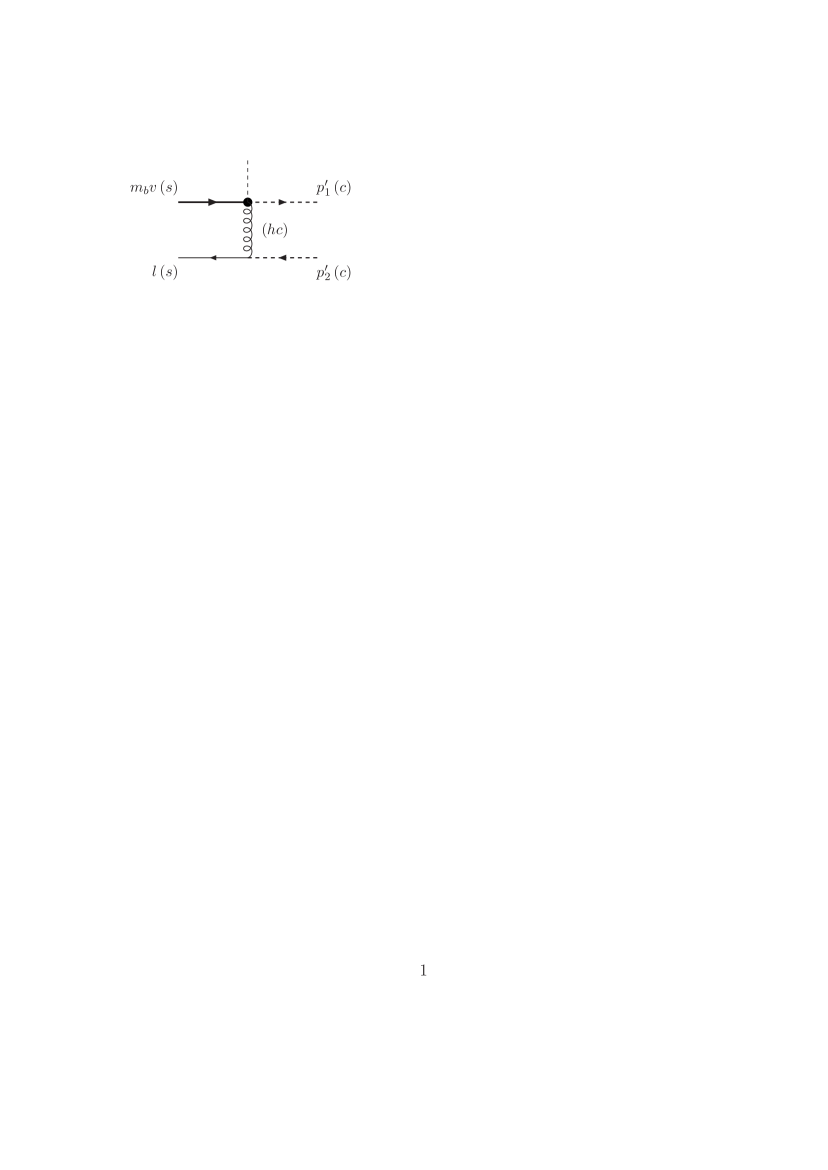
Figure 1: Tree diagram.

The tree contribution to (29) is shown in Figure 1. The gluon momentum (outgoing from the operator vertex) is given by $k=p_{2}^{\prime}-l$, and with $k^{2}=-\bar{v}n_{+}p^{\prime}n_{-}l=-2E\omega\bar{v}$, we obtain

$${\cal A}_{k}^{(0)}(\tau;v,\omega)=-\frac{g_{s}^{2}C_{F}}{N_{c}}\frac{1}{2E\omega\bar{v}}\,\delta(\tau-\bar{v})\,\Gamma_{k}\otimes\gamma_{\perp}^{\mu}\,,$$ (36)

where $\Gamma_{1}\otimes\Gamma_{2}$ means $\bar{u}_{c}(p_{1}^{\prime})\Gamma_{1}u_{h}(m_{b}v)\,\bar{v}(l)\Gamma_{2}v_{c}(p_{2}^{\prime})$. The heavy quark spinor satisfies $v\hskip-4.49997pt/u_{h}(m_{b}v)=u_{h}(m_{b}v)$, and for the collinear spinors $n\hskip-4.49997pt/_{-}v_{c}(p_{2}^{\prime})=\bar{u}_{c}(p_{1}^{\prime})n\hskip-4.49997pt/_{-}=0$.

3.2.2 One loop

A generic 1-loop diagram in SCET_I contains contributions from the hard-collinear, collinear and soft momentum region. For our external momentum configuration soft and collinear loop integrals are scaleless, so the diagram computation extracts the hard-collinear contribution. The SCET_I diagrams are shown in Figure 2, omitting diagrams that are obviously scaleless. We use dimensional regularization ($d=4-2\epsilon$) for both ultraviolet and infrared singularities, hence scaleless integrals vanish.

Figure 2: 1-loop diagrams. The first diagram summarizes all gluon propagator corrections. Diagrams without numbers are omitted when the calculation is done by expansion of QCD diagrams.

We computed the 1-loop diagrams in two different ways. First, we used the SCET_I Feynman rules as given above and computed the diagrams as shown in the figure. Second, we computed the matrix element (29) with full QCD Feynman rules, but expanded the Feynman integrand under the assumption that the loop momentum is hard-collinear, and the external momenta collinear and soft, respectively. This method, also known as the “strategy of expanding by regions” [25, 26], gives precisely the same result as the first computation, but it turns out to be algebraically simpler, because it avoids having to use the more complicated vertex Feynman rules generated by the SCET Lagrangian. There are also fewer diagrams to compute. There are no two-gluon $q\bar{q}gg$ vertices in full QCD, and the unnumbered diagrams in Figure 2 are absent. In both computations we write

$$\frac{d^{d}k}{(2\pi)^{d}}=\frac{1}{8\pi^{2}}\,dn_{+}kdn_{-}k\,\frac{d^{d-2}k_{\perp}}{(2\pi)^{d-2}},$$ (37)

and first perform the $n_{-}k$-integral by contour integration. The $k_{\perp}$-integral reduces to a conventional Feynman integral; the $n_{+}k$-integration is eliminated by the $\delta$-function in (30) or (31) with the exception of diagrams such as (1), (5) or (6).

It is convenient to perform the calculation without specifying the Dirac matrix $\Gamma_{k}$ of the SCET_I operator. The unrenormalized matrix element (29) can be written as

$${\cal A}_{k}^{(ur)} = \Big{[}A^{(0)}\!+A^{(1)}\Big{]}\,\Gamma_{k}\otimes\gamma^{\mu_{\perp}}+B^{(1)}\gamma^{\rho_{\perp}}\gamma^{\mu_{\perp}}\Gamma_{k}\otimes\gamma_{\rho_{\perp}}+C^{(1)}\gamma^{\rho_{\perp}}\gamma^{\lambda_{\perp}}\Gamma_{k}\otimes\gamma^{\mu_{\perp}}\gamma_{\lambda_{\perp}}\gamma_{\rho_{\perp}}\hskip 19.91684pt$$ (38)

in terms of Dirac structures that cannot be reduced further in $d$ dimensions. The notation is such that for any quantity the superscript (0) denotes the tree and (1) the 1-loop contribution. The coefficients of all three structures are infrared divergent, but only $A^{(1)}$ and $B^{(1)}$ are ultraviolet divergent. It follows that all B-type currents can be renormalized with only two independent renormalization constants. Specifically, inserting the three Dirac structures (17), we obtain

$${\cal A}_{1}^{(ur)} = \left[A+(d-2)B\right]\,(\gamma_{5})\gamma_{\mu_{\perp}}\otimes\gamma^{\mu_{\perp}}+C\,(\gamma_{5})\gamma^{\rho_{\perp}}\gamma^{\lambda_{\perp}}\gamma^{\mu_{\perp}}\otimes\gamma_{\mu_{\perp}}\gamma_{\lambda_{\perp}}\gamma_{\rho_{\perp}},$$

$${\cal A}_{2}^{(ur)} = A\,(\gamma_{5})\gamma_{\nu_{\perp}}\gamma_{\mu_{\perp}}\otimes\gamma^{\mu_{\perp}}+(4-d)B\,(\gamma_{5})\gamma_{\mu_{\perp}}\gamma_{\nu_{\perp}}\otimes\gamma^{\mu_{\perp}}$$

$$\hskip 28.45274pt+\,C\,(\gamma_{5})\gamma^{\rho_{\perp}}\gamma^{\lambda_{\perp}}\gamma_{\nu_{\perp}}\gamma^{\mu_{\perp}}\otimes\gamma_{\mu_{\perp}}\gamma_{\lambda_{\perp}}\gamma_{\rho_{\perp}},$$

$${\cal A}_{3}^{(ur)} = \left[A+(d-2)B\right]\,(\gamma_{5})\gamma_{\mu_{\perp}}\gamma_{\nu_{\perp}}\otimes\gamma^{\mu_{\perp}}+C\,(\gamma_{5})\gamma^{\rho_{\perp}}\gamma^{\lambda_{\perp}}\gamma^{\mu_{\perp}}\gamma_{\nu_{\perp}}\otimes\gamma_{\mu_{\perp}}\gamma_{\lambda_{\perp}}\gamma_{\rho_{\perp}}.\phantom{--}$$ (39)

Here and in the following we use anti-commuting $\gamma_{5}$, and the bracket around $\gamma_{5}$ refers to the two cases, where $\gamma_{5}$ is or is not included in $\Gamma_{k}$. From this it can be seen that the UV divergent parts have the same Dirac structure as the original operator. Hence, the operators ${\cal J}_{k}(\tau)$ and all the B-type current operators do not mix under renormalization (in the basis adopted here). The renormalization constant for the operator ${\cal J}_{k}(\tau)$ with $\Gamma_{1,3}$ is related to the divergent part of $A^{(1)}+2B^{(1)}$, the one for ${\cal J}_{k}(\tau)$ with $\Gamma_{2}$ to $A^{(1)}$.

3.3 Ultraviolet counterterms

The counterterm diagrams are obtained from the tree diagram by insertions of a counterterm vertex into the gluon propagator, the quark gluon vertex and the operator vertex. Finally, the on-shell matrix element must be multiplied by the propagator residue factors $R_{h_{v}}^{1/2}R_{q_{s}}^{1/2}R_{\xi}$. They are related to the field renormalization constants by

$$R_{X}=\frac{Z_{X}^{\rm OS}}{Z_{X}},$$ (40)

where $Z_{X}^{\rm OS}$ is the renormalization constant of field $X$ in the on-shell scheme (by definition $R_{X}^{\rm OS}=1$) and $Z_{X}$ is the field renormalization constant in the $\overline{\rm MS}$ scheme.

The Lagrangian counterterms are standard. As regards the operator counterterms, we note that the three operators ${\cal J}_{k}(\tau)$ do not mix (see above), hence the renormalized operator is related to the bare operator (expressed in terms of bare fields) by

$${\cal J}_{1,3}(\tau) = \int d\tau^{\prime}\,Z_{\parallel}(\tau,\tau^{\prime})\,{\cal J}_{1,3}^{\rm bare}(\tau^{\prime}),$$

$${\cal J}_{2}(\tau) = \int d\tau^{\prime}\,Z_{\perp}(\tau,\tau^{\prime})\,{\cal J}_{2}^{\rm bare}(\tau^{\prime}),$$ (41)

which defines the operator renormalization kernels. Here we used that ${\cal J}_{1}(\tau)$ and ${\cal J}_{3}(\tau)$ renormalize identically.

Putting together all the renormalization constants, the on-shell ultraviolet-renormalized matrix elements of ${\cal J}_{1}$ and ${\cal J}_{3}$ follow from (39) by the replacement

$$A+(d-2)B \to A+(d-2)B+Z_{\parallel}^{(1)}\star A^{(0)}$$ (42)

$$+\,\Big{(}2Z_{g}^{(1)}+\frac{1}{2}\,\Big{(}Z_{h_{v}}^{{\rm OS}(1)}+Z_{q_{s}}^{{\rm OS}(1)}+2Z_{\xi}^{{\rm OS}(1)}\Big{)}\Big{)}\,A^{(0)},$$

while the renormalized matrix element of $J_{2}$ is the second line of (39) with

$$A \to A+Z_{\perp}^{(1)}\star A^{(0)}$$ (43)

$$+\,\Big{(}2Z_{g}^{(1)}+\frac{1}{2}\,\Big{(}Z_{h_{v}}^{{\rm OS}(1)}+Z_{q_{s}}^{{\rm OS}(1)}+2Z_{\xi}^{{\rm OS}(1)}\Big{)}\Big{)}\,A^{(0)}.$$

The asterisk denotes convolution in the variable $\tau^{\prime}$ as in the definition of the operator renormalization kernels. The on-shell field renormalization factors are all equal to 1 in dimensional regularization, so $Z_{X}^{{\rm OS}(1)}=0$. $Z_{g}$ is the standard $\overline{\rm MS}$ strong coupling renormalization factor, $g_{s}^{\rm bare}=Z_{g}g_{s}$ with ($C_{A}=3$, $T_{f}=1/2$)

$$Z_{g}=1-\frac{\alpha_{s}\beta_{0}}{8\pi\epsilon},\qquad\beta_{0}=\frac{11C_{A}}{3}-\frac{4}{3}n_{f}T_{f}.$$ (44)

The matrix elements (39) with the substitutions (42), (43) are now ultraviolet finite, but infrared divergent. The infrared divergences are reproduced by the SCET_II computation of the matrix element, resulting in a finite jet-function. This can be used to determine the operator renormalization kernels $Z_{\parallel}$ and $Z_{\perp}$ alternative to the direct computation of the operators’ ultraviolet singularities performed in [20]. That is, after extracting the jet-function, we shall obtain the renormalization factors by requiring that they render the result finite.

3.4 Matching to SCET_II and extraction of the jet function

3.4.1 SCET_II matrix element

To obtain the jet-function, we need the SCET_II matrix elements on the right hand side of the matching equation (28) to the 1-loop order. In the absence of collinear-soft interactions in SCET_II the four-quark operator factorizes into a collinear and a soft bilinear. We define

$$Q[\Gamma_{k}^{c}](v) = \Big{[}(\bar{\xi}W_{c})(sn_{+})\frac{n\hskip-4.49997pt/_{+}}{2}\Gamma^{c}_{k}(W_{c}^{\dagger}\xi)(0)\Big{]}_{\rm FT}$$

$$= \frac{n_{+}p^{\prime}}{2\pi}\int ds\,e^{-isvn_{+}p^{\prime}}\,(\bar{\xi}W_{c})(sn_{+})\frac{n\hskip-4.49997pt/_{+}}{2}\Gamma^{c}_{k}(W_{c}^{\dagger}\xi)(0),$$

$$P(\omega) = \Big{[}(\bar{q}_{s}Y_{s})(tn_{-})\frac{n\hskip-4.49997pt/_{-}}{2}\gamma_{5}(Y_{s}^{\dagger}h_{v})(0)\Big{]}_{\rm FT}$$ (45)

$$= \frac{1}{2\pi}\int dt\,e^{it\omega}\,(\bar{q}_{s}Y_{s})(tn_{-})\frac{n\hskip-4.49997pt/_{-}}{2}\gamma_{5}(Y_{s}^{\dagger}h_{v})(0),$$

and the quark matrix elements

$$\Phi_{q\bar{q}}(v^{\prime},v) = \langle q(p_{1}^{\prime})\bar{q}(p_{2}^{\prime})|Q[\Gamma_{k}^{c}](v^{\prime})|0\rangle,$$

$$\Phi_{b\bar{q}}(\omega^{\prime},\omega) = \langle 0|P(\omega^{\prime})|\bar{q}(l)b_{v}(0)\rangle.$$ (46)

The Dirac matrices $\Gamma_{k}^{c}$ will be determined later by the Fierz transformation of the first Dirac matrix product on the right-hand sides of (39). Note that the hadronic matrix elements of $Q$ and $P$ are precisely the meson light-cone distribution amplitudes. Collinear-soft factorization in SCET_II means that the matrix element of $Q[\Gamma_{k}^{c}](v)P(\omega)$, which appears in (28), factorizes into

$$\langle M(p^{\prime})|Q[\Gamma_{k}^{c}](v)P(\omega)|\bar{B}_{v}\rangle=\langle M(p^{\prime})|Q[\Gamma_{k}^{c}](v)|0\rangle\langle 0|P(\omega)|\bar{B}_{v}\rangle,$$ (47)

which is a product of light-cone distribution amplitudes.

With these definitions the tree quark matrix element of the SCET_II four-quark operator is given by

$$\langle q(p_{1}^{\prime})\bar{q}(p_{2}^{\prime})|Q[\Gamma_{k}^{c}](v^{\prime})P(\omega^{\prime})|\bar{q}(l)b(m_{b}v)\rangle^{(0)}=\delta(v-v^{\prime})\delta(\omega-\omega^{\prime})\,\frac{n\hskip-4.49997pt/_{+}}{2}\Gamma^{c}_{k}\,\tilde{\otimes}\,\frac{n\hskip-4.49997pt/_{-}}{2}\gamma_{5},$$ (48)

where now $\Gamma_{1}\,\tilde{\otimes}\,\Gamma_{2}$ means $\bar{u}_{c}(p_{1}^{\prime})\Gamma_{1}v_{c}(p_{2}^{\prime})\,\bar{v}(l)\Gamma_{2}u_{h}(m_{b}v)$. The “tensor products” $\otimes$ and $\tilde{\otimes}$ are related by a Fierz transformation as discussed below.

The SCET_II computation of the matrix elements (46) is very simple, since in the collinear sector SCET_II is equivalent to full QCD, and in the soft sector to heavy quark effective theory [12]. The external momenta do not allow to form a non-vanishing kinematic invariant, hence all loop integrals are scaleless and vanish. The matrix elements are given by tree diagrams including tree diagrams with counterterm insertions. We can therefore write

$$\Phi_{q\bar{q}}(v^{\prime},v) = Z_{Q}(v^{\prime},v)\,\frac{n\hskip-4.49997pt/_{+}}{2}\Gamma^{c}_{k},$$

$$\Phi_{b\bar{q}}(\omega^{\prime},\omega) = Z_{P}(\omega^{\prime},\omega)\,\frac{n\hskip-4.49997pt/_{-}}{2}\gamma_{5},$$ (49)

with $Z_{Q}(v^{\prime},v)$ and $Z_{P}(\omega^{\prime},\omega)$ the renormalization kernels that relate the renormalized operator to the bare operator expressed in terms of the bare fields,

$$Q[\Gamma_{k}^{c}](v) = \int_{0}^{1}dw\,Z_{Q}(v,w)\,Q[\Gamma_{k}^{c}]^{\rm bare}(w),$$

$$P(\omega) = \int_{0}^{1}d\omega^{\prime}\,Z_{P}(\omega,\omega^{\prime})\,P^{\rm bare}(\omega^{\prime}).$$ (50)

The required 1-loop renormalization factors have been computed in other contexts. For the collinear operator $Z_{Q}(v,w)$ is the Brodsky-Lepage kernel [28]

$$Z_{Q}(v,w) = \delta(v-w)+Z_{Q}^{(1)}(v,w)+\ldots,$$

$$Z_{Q}^{(1)}(v,w) = -\frac{\alpha_{s}C_{F}}{2\pi\epsilon}\,\Bigg{\{}\frac{1}{w\bar{w}}\left[v\bar{w}\frac{\theta(w-v)}{w-v}+\bar{v}w\frac{\theta(v-w)}{v-w}\right]_{+}$$ (51)

$$-\,\frac{1}{2}\,\delta(v-w)+\Delta\left(\frac{v}{w}\theta(w-v)+\frac{\bar{v}}{\bar{w}}\theta(v-w)\right)\Bigg{\}},$$

where $\Delta=1$ applies to $\Gamma_{k}^{c}=(\gamma_{5})1$ (pseudoscalar meson, longitudinally polarized vector meson distribution amplitudes) and $\Delta=0$ to $\Gamma_{k}^{c}=\gamma_{\perp}^{\nu}$ (transversely polarized vector meson distribution amplitude), and the plus-distribution is defined for symmetric kernels $f$ as

$$\int dw[f(v,w)]_{+}\,g(w)=\int dwf(v,w)\,\left(g(w)-g(v)\right).$$ (52)

Similarly, the renormalization of $P(\omega)$ has been worked out in [29] with the result

$$Z_{P}(\omega,\omega^{\prime}) = \delta(\omega-\omega^{\prime})+Z_{P}^{(1)}(\omega,\omega^{\prime})+\ldots,$$

$$Z_{P}^{(1)}(\omega,\omega^{\prime}) = \frac{\alpha_{s}C_{F}}{4\pi}\,\Bigg{[}\left(\frac{1}{\epsilon^{2}}+\frac{2}{\epsilon}\,\ln\frac{\mu}{\omega}-\frac{5}{2\epsilon}\right)\delta(\omega-\omega^{\prime})$$ (53)

$$-\,\frac{2\omega}{\epsilon}\left(\frac{1}{\omega^{\prime}}\,\frac{\theta(\omega^{\prime}-\omega)}{\omega^{\prime}-\omega}+\frac{1}{\omega}\,\frac{\theta(\omega-\omega^{\prime})}{\omega-\omega^{\prime}}\right)_{+}\Bigg{]}.$$

3.4.2 Extraction of the jet-function

The jet-function is extracted from the quark matrix element of (28),

$${\cal A}_{k}(\tau;v,\omega)=\int_{0}^{\infty}d\omega^{\prime}\int_{0}^{1}dv^{\prime}\,J_{k}(\tau;\omega^{\prime},v^{\prime})\,\Phi_{b\bar{q}}(\omega^{\prime},\omega)\,\Phi_{q\bar{q}}(v^{\prime},v).$$ (54)

This gives

$$J_{k}^{(0)}(\tau;\omega,v)\,\frac{n\hskip-4.49997pt/_{+}}{2}\tilde{\Gamma}_{k}^{c}\tilde{\otimes}\,\frac{n\hskip-4.49997pt/_{-}}{2}\gamma_{5}={\cal A}^{(0)}(\tau;v,\omega),$$ (55)

at tree level, and

$$J_{k}^{(1)}(\tau;\omega,v)\,\frac{n\hskip-4.49997pt/_{+}}{2}\tilde{\Gamma}_{k}^{c}\tilde{\otimes}\,\frac{n\hskip-4.49997pt/_{-}}{2}\gamma_{5} = {\cal A}_{k}^{(1)}(\tau;v,\omega)-\bigg{[}\int_{0}^{\infty}d\omega^{\prime}\,Z_{P}^{(1)}(\omega^{\prime},\omega)\,J_{k}^{(0)}(\tau;\omega^{\prime},v)$$ (56)

$$+\,\int_{0}^{1}dv^{\prime}\,Z_{Q}^{(1)}(v^{\prime},v)\,J_{k}^{(0)}(\tau;\omega,v^{\prime})\bigg{]}\,\frac{n\hskip-4.49997pt/_{+}}{2}\tilde{\Gamma}_{k}^{c}\tilde{\otimes}\,\frac{n\hskip-4.49997pt/_{-}}{2}\gamma_{5}$$

at the 1-loop order. ${\cal A}_{k}^{(1)}(\tau;v,\omega)$ is the ultraviolet-renormalized but infrared divergent 1-loop matrix element of ${\cal J}_{k}(\tau)$. The subtraction on the right-hand side precisely cancels the infrared divergences, so that the short-distance jet-function is finite as it should be. There is however a difficulty in executing the subtraction in the form of (56), since ${\cal A}_{k}^{(1)}(\tau;v,\omega)$ is expressed in terms of the spinor product $\otimes$, corresponding to SCET_II operators with spinor indices contracted in $[\bar{\xi}h_{v}]\,[\bar{q}_{s}\xi]$, while the left-hand side and the subtraction term involve the product $\tilde{\otimes}$, corresponding to operators with spinor indices contracted in $[\bar{\xi}\xi]\,[\bar{q}_{s}h_{v}]$. The standard Fierz identities that relate these structures are valid only in four dimensions. We shall discuss this issue together with the reduction of evanescent Dirac structures appearing in (39) in the following subsection.

None of this applies to the tree-level equation (55), where all quantities are finite. We can therefore apply the four-dimensional Fierz identities to the tree-level terms in (39), so that for

$$k=1:\qquad (\gamma_{5})\gamma_{\mu_{\perp}}\otimes\gamma^{\mu_{\perp}}=(\pm 1)\,\frac{n\hskip-5.89996pt/_{+}}{2}\gamma_{5}(\gamma_{5})\,\tilde{\otimes}\,\frac{n\hskip-5.89996pt/_{-}}{2}\gamma_{5}+\ldots,$$ (57)

$$k=2:\qquad (\gamma_{5})\gamma_{\nu_{\perp}}\gamma_{\mu_{\perp}}\otimes\gamma^{\mu_{\perp}}=-\frac{n\hskip-5.89996pt/_{+}}{2}\gamma_{\nu_{\perp}}\gamma_{5}(\gamma_{5})\,\tilde{\otimes}\,\frac{n\hskip-5.89996pt/_{-}}{2}\gamma_{5}+\ldots,$$

$$k=3:\qquad (\gamma_{5})\gamma_{\mu_{\perp}}\gamma_{\nu_{\perp}}\otimes\gamma^{\mu_{\perp}}=\ldots.$$

The Fierz transformation produces a number of 4-fermion operators with different Dirac structures. In the following we discuss only those operators (jet-functions) that contribute to the decay of a pseudoscalar $\bar{B}$ meson. The ellipses denote terms involving $n\hskip-5.89996pt/_{-}/2$ and $n\hskip-5.89996pt/_{-}/2\,\gamma_{\nu_{\perp}}(\gamma_{5})$ to the right of $\tilde{\otimes}$, which vanish when the matrix element $\langle 0|\bar{q}_{s}[\ldots]h_{v}|\bar{B}\rangle$ with the pseudoscalar $\bar{B}$ meson state is evaluated. Hence, these terms will not be considered further. The upper (lower) sign refers to the operators on the left-hand side without (with) the $\gamma_{5}$ factor. Here and below the Fierz identities are given for four-fermion operators and the extra minus sign from the field permutation relative to the identities for matrix products is already included. Comparison of (57) with the definition (45) of $Q[\Gamma_{k}^{c}]$ determines the Dirac matrix $\Gamma_{k}^{c}$ in the collinear SCET_II operator. For $k=1$, we have $\Gamma_{k}=(\gamma_{5})\gamma_{\mu_{\perp}}$ and the corresponding $\tilde{\Gamma}_{k}^{c}=(\pm 1)\gamma_{5}(\gamma_{5})$; for $k=2$, $\Gamma_{k}=(\gamma_{5})\gamma_{\nu_{\perp}}\gamma_{\mu_{\perp}}$ and $\tilde{\Gamma}_{k}^{c}=-\gamma_{\nu_{\perp}}\gamma_{5}(\gamma_{5})$; for $k=3$, $\Gamma_{k}=(\gamma_{5})\gamma_{\mu_{\perp}}\gamma_{\nu_{\perp}}$ and $\tilde{\Gamma}_{k}^{c}=0$, i.e. there is no contribution for pseudoscalar $B$ mesons. Hence, comparing (55), (57) to (36) leads to the tree-level jet function

$$J_{k}^{(0)}(\tau;v,\omega)=-\frac{g_{s}^{2}C_{F}}{N_{c}}\frac{1}{2E\omega\bar{v}}\,\delta(\tau-\bar{v})$$ (58)

for $k=1,2$, and 0 for $k=3$.

Using the 1-loop expressions for the SCET_II renormalization kernels, we can evaluate the subtraction term in square brackets in (56) with the result

$$-\frac{g_{s}^{2}C_{F}}{N_{c}}\,\frac{1}{2E\omega\bar{v}}\,\left\{\frac{\alpha_{s}C_{F}}{4\pi}\,\delta(\tau-\bar{v})\left(\frac{1}{\epsilon^{2}}+\frac{2}{\epsilon}\ln\frac{\mu}{\omega}-\frac{5}{2\epsilon}\right)+\frac{\bar{v}}{\tau}Z_{Q}^{(1)}(\bar{\tau},v)\right\}.$$ (59)

3.4.3 Evanescent operators and Fierz transformation

We now discuss the reduction of the Dirac structure and the Fierz transformation. We consider in detail the case $\Gamma_{k}=\gamma^{\mu_{\perp}}$. According to the first equation of (39) the UV renormalized matrix element of the corresponding SCET_I current ${\cal J}_{1}(\tau)$ is

$${\cal A}_{1}(\tau;v,\omega)=\hat{A}\,\gamma_{\mu_{\perp}}\otimes\gamma^{\mu_{\perp}}+C\,\gamma^{\rho_{\perp}}\gamma^{\lambda_{\perp}}\gamma^{\mu_{\perp}}\otimes\gamma_{\mu_{\perp}}\gamma_{\lambda_{\perp}}\gamma_{\rho_{\perp}},$$ (60)

where $\hat{A}$ stands for the right hand side of (42). The second Dirac structure reduces to a multiple of the first one in four dimensions, and the first one satisfies the Fierz relation (57) in four dimensions. In the following we discuss separately the reduction of the Dirac structure and the Fierz transformation in $d$ dimensions, although it is possible to perform both reductions in a single step.

Indicating only the field content and Dirac structure we define the operators $O_{1}=(\bar{\xi}\gamma_{\mu_{\perp}}h_{v})(\bar{q}_{s}\gamma^{\mu_{\perp}}\xi)$ and $O_{1}^{\prime}=(\bar{\xi}\gamma^{\rho_{\perp}}\gamma^{\lambda_{\perp}}\gamma^{\mu_{\perp}}h_{v})(\bar{q}_{s}\gamma_{\mu_{\perp}}\gamma_{\lambda_{\perp}}\gamma_{\rho_{\perp}}\xi)$, and rewrite the previous equation as

$${\cal A}_{1}(\tau;v,\omega)=\left[\hat{A}^{(0)}+\hat{A}^{(1)}\right]\langle O_{1}\rangle^{(0)}+C^{(1)}\langle O_{1}^{\prime}\rangle^{(0)},$$ (61)

where the tree-level matrix elements of $O_{1}^{(\prime)}$ just reproduce the Dirac structures, i.e. $\langle O_{1}\rangle^{(0)}=\bar{u}_{c}(p_{1}^{\prime})\gamma^{\mu_{\perp}}u_{h}(m_{b}v)\,\bar{v}(l)\gamma_{\mu_{\perp}}v_{c}(p_{2}^{\prime})$ etc. In $d=4$, $O_{1}^{\prime}=4O_{1}$, so we define the evanescent operator $E=O_{1}^{\prime}-f(\epsilon)O_{1}$, where $f(0)=4$, but otherwise $f(\epsilon)$ is arbitrary. Hence,

$${\cal A}_{1}(\tau;v,\omega)=\left[\hat{A}^{(0)}+\hat{A}^{(1)}+f(\epsilon)C^{(1)}\right]\langle O_{1}\rangle^{(0)}+C^{(1)}\langle E\rangle^{(0)}.$$ (62)

Since $C^{(1)}$ has a $1/\epsilon$ infrared divergence, the coefficient of the “physical” operator $O_{1}$ depends on the up to now arbitrary prescription $f(\epsilon)$ in the definition of the evanescent operator. The jet-functions are obtained by expressing this equation in terms of the renormalized operator matrix elements. To the 1-loop order it is sufficient to use

$$\langle O_{1}\rangle=\left(1+M_{O_{1}}^{(1)}\right)\langle O_{1}\rangle^{(0)}+M_{O_{1}E}^{(1)}\langle E\rangle^{(0)},\qquad\langle E\rangle=\langle E^{(0)}\rangle,$$ (63)

which results in

$${\cal A}_{1}(\tau;v,\omega) = \left[\hat{A}^{(0)}+\hat{A}^{(1)}+f(\epsilon)C^{(1)}-\hat{A}^{(0)}M_{O_{1}}^{(1)}\right]\langle O_{1}\rangle+\left[C^{(1)}-\hat{A}^{(0)}M_{O_{1}E}^{(1)}\right]\langle E\rangle$$ (64)

$$\stackrel{{\scriptstyle d\to 4}}{{\to}} \left[J_{O_{1}}^{(0)}+J_{O_{1}}^{(1)}\right]\langle O_{1}\rangle.$$

The coefficients of the operator matrix elements in the first line of this equation are now infrared-finite short-distance quantities, and the equation is interpreted as an operator matching relation valid also when the matrix elements are taken between hadronic final states. Hence we can take the limit $d\to 4$ in which $\langle E\rangle=0$, since the tree-level matrix element vanishes in four dimensions. The 1-loop jet-function $J_{O_{1}}^{(1)}$ can be read off from (64). It depends on the choice of the evanescent operator, i.e. the order-$\epsilon$ term of $f(\epsilon)$, but so does $\langle O_{1}\rangle$ as can be seen from (63), and the physical amplitude is scheme-independent.

The jet-function $J_{O_{1}}$ is not the desired result, because instead of $O_{1}$ we must use the Fierz-transformed operator

$$P_{1}=\Big{(}\bar{\xi}\frac{n\hskip-5.89996pt/_{+}}{2}\gamma_{5}\,\xi\Big{)}\,\Big{(}\bar{q}_{s}\frac{n\hskip-5.89996pt/_{-}}{2}\gamma_{5}h_{v}\Big{)}+\ldots,$$ (65)

where the ellipses denote terms that are irrelevant for us, as in (57). This Fierz-ordering is uniquely singled out by collinear-soft factorization in SCET_II. Radiative corrections to $P_{1}$ occur only within the collinear factor or within the soft factor, hence the Dirac structures in arbitrary loop diagrams can be reduced to the tree structure $P_{1}$. It follows that whatever evanescent operator one may write down in this Fierz-ordering decouples from $P_{1}$, and can simply be ignored. Hence, even in $d$ dimensions we have

$${\cal A}_{1}(\tau;v,\omega)=\left[J_{P_{1}}^{(0)}+J_{P_{1}}^{(1)}\right]\langle P_{1}\rangle,$$ (66)

with $J_{P_{1}}^{(1)}$ the desired 1-loop jet-function. Comparing this equation to (64) we have $J_{P_{1}}=J_{O_{1}}$, if the renormalized matrix elements $\langle P_{1}\rangle$ and $\langle O_{1}\rangle$ are equal. In general this is not the case, because the Fierz identity that relates $O_{1}$ and $P_{1}$ in four dimensions is not valid for $d\not=4$. Now, the renormalization scheme for $P_{1}$ is fixed by the requirement that the collinear and soft matrix elements coincide with the standard $\overline{\rm MS}$ definition of the light meson and heavy meson light-cone distribution amplitudes, respectively, so $\langle P_{1}\rangle$ is completely defined. However, by choosing $f(\epsilon)$, we can adjust the definition of $O_{1}$, such that the infrared-finite matrix elements are equal in the limit $d\to 4$.

Since the jet-functions are independent of the infrared regularization, any one can be chosen for the calculation, and it is convenient to compare the matrix elements of $O_{1}$ and $P_{1}$ by assuming an off-shell infrared regularization. The ultraviolet-renormalized 1-loop matrix elements are

$$\langle O_{1}\rangle = \left(1+M_{O_{1}}^{\rm off}\right)\langle O_{1}\rangle^{(0)}+M_{O_{1}E}^{\rm off}\langle E\rangle^{(0)},$$

$$\langle P_{1}\rangle = \left(1+M_{P_{1}}^{\rm off}\right)\langle P_{1}\rangle^{(0)}.$$ (67)

There are no $1/\epsilon$ poles in these equations due to the use of off-shell IR regularization, so the evanescent term drops out for $d\to 4$. Furthermore, $\langle O_{1}\rangle^{(0)}=\langle P_{1}\rangle^{(0)}$ by the four-dimensional Fierz-equivalence of $O_{1}$ and $P_{1}$, hence we need to define $O_{1}$ such that the difference $M_{O_{1}}^{\rm off}-M_{P_{1}}^{\rm off}=0$. At the 1-loop order one finds that the self-energy corrections and the vertex correction, where the gluon is exchanged between the soft light quark and the heavy quark, drop out, because the coupling to the heavy quark is proportional to $v^{\mu}$ and does not introduce a new Dirac structure. Only the gluon exchange between the collinear $\xi$-fields can give a non-zero difference. In the case of $O_{1}$ the part of this diagram that does not cancel in the difference $M_{O_{1}}^{\rm off}-M_{P_{1}}^{\rm off}$ involves $\gamma^{\rho_{\perp}}\gamma^{\lambda_{\perp}}\gamma^{\mu_{\perp}}\otimes\gamma_{\mu_{\perp}}\gamma_{\lambda_{\perp}}\gamma_{\rho_{\perp}}$, and its contribution to $M_{O_{1}}$ is therefore proportional to $f(\epsilon)$. In the case of $P_{1}$, the Dirac structure is

$$\gamma^{\alpha_{\perp}}\gamma^{\beta_{\perp}}\frac{n\hskip-5.89996pt/_{+}}{2}\gamma_{\beta_{\perp}}\gamma_{\alpha_{\perp}}\tilde{\otimes}\frac{n\hskip-5.89996pt/_{-}}{2}=(d-2)^{2}\langle P_{1}\rangle^{(0)}.$$ (68)

Including the overall coefficient, we find

$$M_{O_{1}}^{\rm off}-M_{P_{1}}^{\rm off}=-[C^{(1)}]_{\rm div}\left(f(\epsilon)-(d-2)^{2}\right)\langle P_{1}^{(0)}\rangle$$ (69)

where $[C^{(1)}]_{\rm div}$ is the divergent part of $C^{(1)}$. In order for this to vanish, we must choose $f(\epsilon)=(d-2)^{2}$. In other words, we must define

$$\gamma^{\rho_{\perp}}\gamma^{\lambda_{\perp}}\gamma^{\mu_{\perp}}\otimes\gamma_{\mu_{\perp}}\gamma_{\lambda_{\perp}}\gamma_{\rho_{\perp}}=(d-2)^{2}\,\gamma^{\mu_{\perp}}\otimes\gamma_{\mu_{\perp}}.$$ (70)

With this $J_{P_{1}}=J_{O_{1}}$, so returning to (64) we have

$$J_{P_{1}}^{(1)}=\lim_{d\to 4}\left(\hat{A}^{(1)}+(d-2)^{2}C^{(1)}-\hat{A}^{(0)}M_{P_{1}}^{(1)}\right).$$ (71)

The term $\hat{A}^{(0)}M_{P_{1}}^{(1)}$ is nothing but the subtraction term (59) that appears in (56), while $\hat{A}^{(1)}$ and $C^{(1)}$ can be read off from the 1-loop calculation that leads to (38) and (42), so the previous equation gives the final result for the correctly renormalized and subtracted jet-function. The above argument can be repeated for $\Gamma_{k}=\gamma_{5}\gamma^{\mu_{\perp}}$, and one finds that the jet-function is identical to the one for $\Gamma_{k}=\gamma^{\mu_{\perp}}$ as was expected.

The case of B-type currents ${\cal J}_{2,3}(\tau)$ with one uncontracted transverse index is slightly more complicated than the scalar case, because there are two physical and two evanescent operators. Corresponding to $\Gamma_{k}=(\gamma_{5})\gamma^{\nu_{\perp}}\gamma^{\mu_{\perp}}$ and $(\gamma_{5})\gamma^{\mu_{\perp}}\gamma^{\nu_{\perp}}$ we define the two physical operators $O_{2}=(\bar{\xi}(\gamma_{5})\gamma_{\nu_{\perp}}\gamma_{\mu_{\perp}}h_{v})(\bar{q}_{s}\gamma^{\mu_{\perp}}\xi)$ and $O_{3}=(\bar{\xi}(\gamma_{5})\gamma_{\mu_{\perp}}\gamma_{\nu_{\perp}}h_{v})(\bar{q}_{s}\gamma^{\mu_{\perp}}\xi)$. Requiring that the renormalized matrix elements of $O_{2,3}$ equal the renormalized matrix elements of the corresponding operators $P_{2,3}$ in the other Fierz-ordering fixes uniquely the prescription for reducing the Dirac structures multiplying $C$ in (39) and ensures that the SCET_II operators are correctly minimally subtracted. A short calculation analogous to the one discussed above gives

$$(\gamma_{5})\gamma^{\rho_{\perp}}\gamma^{\lambda_{\perp}}\gamma_{\nu_{\perp}}\gamma^{\mu_{\perp}}\otimes\gamma_{\mu_{\perp}}\gamma_{\lambda_{\perp}}\gamma_{\rho_{\perp}}=(d-4)^{2}\,(\gamma_{5})\gamma_{\nu_{\perp}}\gamma_{\mu_{\perp}}\otimes\gamma^{\mu_{\perp}},$$

$$(\gamma_{5})\gamma^{\rho_{\perp}}\gamma^{\lambda_{\perp}}\gamma^{\mu_{\perp}}\gamma_{\nu_{\perp}}\otimes\gamma_{\mu_{\perp}}\gamma_{\lambda_{\perp}}\gamma_{\rho_{\perp}}=(d-2)^{2}\,(\gamma_{5})\gamma_{\mu_{\perp}}\gamma_{\nu_{\perp}}\otimes\gamma^{\mu_{\perp}}.$$ (72)

Referring to (57) we see that the matrix element of $O_{3}$ vanishes for a pseudoscalar $\bar{B}$ meson. Hence the B-type operator ${\cal J}_{3}(\tau)$ with $\Gamma_{k}=(\gamma_{5})\gamma_{\mu_{\perp}}\gamma_{\nu_{\perp}}$ has a vanishing jet-function just as at tree level. On the other hand, inserting the first equation of (72) into the second of (39), we find that the B-type operator ${\cal J}_{2}(\tau)$ matches to $J_{P_{2}}P_{2}$ with

$$J_{P_{2}}^{(1)}=\lim_{d\to 4}\left(A^{(1)}+(d-4)^{2}C^{(1)}-A^{(0)}M_{P_{2}}^{(1)}\right).$$ (73)

Here $A^{(1)}$ and $C^{(1)}$ are defined by (39) and (43) and the subtraction term is given by (56) except that now $\Delta=0$ must be used in the Brodsky-Lepage kernel. Since $C^{(1)}$ has only a single $1/\epsilon$ pole, the term $(d-4)^{2}C^{(1)}$ does not contribute to the final result for the jet-function.

3.5 Final results for the jet-functions and B-type current renormalization kernels

We shall now denote the jet-function $J_{P_{1}}$ ($J_{P_{2}}$) that arises in the matching of ${\cal J}_{1}(\tau)$ (${\cal J}_{2}(\tau)$) as $J_{\parallel}$ ($J_{\perp}$). To the 1-loop order we write

$$J_{a} = -\frac{g_{s}^{2}C_{F}}{N_{c}}\,\frac{1}{2E\omega\bar{v}}\left(\delta(\tau-\bar{v})+\frac{\alpha_{s}}{4\pi}\,j_{a}(\tau;v,\omega)\right)$$ (74)

with $a=\,\parallel,\perp$. Applying the subtraction procedure described in the previous subsections we obtain the ultraviolet and infrared finite 1-loop corrections $j_{a}(\tau;v,\omega)$. The resulting expressions still depend on the yet undetermined renormalization factors $Z_{a}^{(1)}$ of the B-type currents through (42), (43). They can now be determined by the condition that $j_{a}(\tau;v,\omega)$ must not contain $1/\epsilon$ poles. We choose the $\overline{\rm MS}$ scheme to be consistent with the definition of the B-type short-distance coefficients in [18].

3.5.1 Renormalization kernels

We expand the $Z$-factors in (41) as

$$Z_{a}(\tau,\tau^{\prime})=\delta(\tau-\tau^{\prime})+\frac{\alpha_{s}}{4\pi}\,z_{a}^{(1)}(\tau,\tau^{\prime}),$$ (75)

and obtain

$$z_{\parallel}^{(1)}(\tau,\tau^{\prime}) = (-C_{F})\left(\frac{1}{\epsilon^{2}}+\frac{2}{\epsilon}\ln\frac{\mu}{2E}\right)\delta(\tau-\tau^{\prime})-\frac{1}{\epsilon}\,\Big{[}z_{1}(\tau,\tau^{\prime})+z_{2}(\tau,\tau^{\prime})\Big{]},$$

$$z_{\perp}^{(1)}(\tau,\tau^{\prime}) = (-C_{F})\left(\frac{1}{\epsilon^{2}}+\frac{2}{\epsilon}\ln\frac{\mu}{2E}\right)\delta(\tau-\tau^{\prime})-\frac{z_{1}(\tau,\tau^{\prime})}{\epsilon},$$ (76)

with

$$z_{1}(\tau,\tau^{\prime}) = \delta(\tau-\tau^{\prime})\left\{C_{F}\left[-2\ln\bar{\tau}+\frac{5}{2}\right]+C_{A}\ln\frac{\bar{\tau}}{\tau}\right\}$$

$$+\,C_{A}\left[\frac{\theta(\tau-\tau^{\prime})}{\tau-\tau^{\prime}}+\frac{\theta(\tau^{\prime}-\tau)}{\tau^{\prime}-\tau}\right]_{+}+\left(C_{F}-\frac{C_{A}}{2}\right)\,\frac{2\bar{\tau}}{\tau\tau^{\prime}}\theta(\tau-\bar{\tau}^{\prime})$$

$$-\,C_{A}\left(\frac{1}{\tau\bar{\tau}^{\prime}}\theta(\tau-\tau^{\prime})+\frac{1}{\tau^{\prime}}\theta(\tau^{\prime}-\tau)\right),$$

$$z_{2}(\tau,\tau^{\prime}) = (-2)\left(C_{F}-\frac{C_{A}}{2}\right)\left(\frac{\tau\tau^{\prime}}{\bar{\tau}^{\prime}}\theta(\bar{\tau}^{\prime}-\tau)+\bar{\tau}\left(1+\frac{1}{\tau}+\frac{1}{\tau^{\prime}}\right)\theta(\tau-\bar{\tau}^{\prime})\right)$$ (77)

$$+\,C_{A}\left(\frac{\bar{\tau}\tau^{\prime}}{\bar{\tau}^{\prime}}\left(1+\frac{1}{\tau}\right)\theta(\tau-\tau^{\prime})+\tau\left(1+\frac{1}{\tau^{\prime}}\right)\theta(\tau^{\prime}-\tau)\right).$$

The anomalous dimensions of the B-type operators are derived from the renormalization kernels in the standard way (see (102) below). Our result is in complete agreement with [20], where the anomalous dimension has been obtained by extracting directly the ultraviolet divergent parts of the SCET_I diagrams.

3.5.2 Jet-functions

The 1-loop jet-functions read

$$j_{\parallel}(\tau;v,\omega) = A\,\delta(\tau-\bar{v})+\bigg{(}C_{F}-\frac{C_{A}}{2}\bigg{)}\,\big{[}2B\big{]}_{+}$$ (78)

$$+\,C_{F}\bigg{[}\theta(\bar{v}-\tau)\,\frac{2\bar{\tau}}{v\bar{v}}\bigg{(}L+\ln\frac{(\bar{v}-\tau)\tau}{\bar{v}}+\frac{v(\bar{v}-\tau)}{\tau\bar{\tau}}\bigg{)}-\frac{2\bar{v}\bar{\tau}}{v}\bigg{(}L+\ln\tau\bar{\tau}+\frac{v\bar{\tau}}{\bar{v}\tau}\bigg{)}\bigg{]}$$

$$-\,\bigg{(}C_{F}-\frac{C_{A}}{2}\bigg{)}\Bigg{[}\theta(\tau-v)\,\frac{2(v-\tau)^{2}}{v\bar{v}\tau}\bigg{(}L+\ln\frac{(\tau-v)\bar{\tau}}{\bar{v}}-\frac{v\bar{\tau}}{(v-\tau)^{2}}\bigg{)}$$

$$+\,\theta(\bar{v}-\tau)\,\frac{2(v-\tau)}{v\bar{v}}\bigg{(}L+\ln(\bar{v}-\tau)+\frac{\tau\bar{\tau}}{(\bar{v}-\tau)(v-\tau)}\ln\frac{\bar{v}}{\tau}-\frac{v}{v-\tau}\bigg{)}$$

$$+\,\theta(\tau-\bar{v})\,\frac{2}{\tau}\bigg{(}L+\ln(\tau-\bar{v})+\frac{\bar{v}}{\tau-\bar{v}}\ln\frac{v}{\bar{\tau}}-\frac{\bar{\tau}}{v}\bigg{)}\Bigg{]},$$

$$j_{\perp}(\tau;v,\omega) = A\,\delta(\tau-\bar{v})+\bigg{(}C_{F}-\frac{C_{A}}{2}\bigg{)}\,\big{[}2B\big{]}_{+}$$ (79)

$$+\,C_{F}\bigg{[}\theta(\bar{v}-\tau)\,\frac{2}{\bar{v}}\bigg{(}L+\ln\frac{(\bar{v}-\tau)\tau}{\bar{v}}-1\bigg{)}-\theta(\tau-\bar{v})\,\frac{2\bar{\tau}}{v\tau}\bigg{]}$$

$$-\,\bigg{(}C_{F}-\frac{C_{A}}{2}\bigg{)}\Bigg{[}\theta(\tau-v)\,\frac{2\bar{\tau}}{\bar{v}\tau}\bigg{(}L+\ln\frac{(\tau-v)\bar{\tau}}{\bar{v}}-\frac{v-\tau}{v\bar{\tau}}\bigg{)}$$

$$+\,\theta(\bar{v}-\tau)\,\frac{2}{\bar{v}}\bigg{(}L+\ln(\bar{v}-\tau)+\frac{\tau}{\bar{v}-\tau}\ln\frac{\bar{v}}{\tau}-\frac{1}{v}\bigg{)}$$

$$+\,\theta(\tau-\bar{v})\,\frac{2}{v\tau}\bigg{(}L+\ln(\tau-\bar{v})+\frac{\bar{v}\bar{\tau}}{\tau-\bar{v}}\ln\frac{v}{\bar{\tau}}-1\bigg{)}\Bigg{]}$$

with

$$A = C_{F}\bigg{[}\Big{(}L+\ln\bar{v}\Big{)}^{2}-\frac{13}{3}\Big{(}L+\ln\bar{v}\Big{)}-\frac{\pi^{2}}{6}+\frac{80}{9}\bigg{]}$$

$$+\,\bigg{(}C_{F}-\frac{C_{A}}{2}\bigg{)}\bigg{[}\Big{(}L+\ln v\Big{)}^{2}-\Big{(}L+\ln\bar{v}\Big{)}^{2}+\frac{22}{3}\Big{(}L+\ln\bar{v}\Big{)}+\frac{2\pi^{2}}{3}-\frac{152}{9}\bigg{]}$$

$$+\,n_{f}T_{f}\bigg{[}\frac{4}{3}\Big{(}L+\ln\bar{v}\Big{)}-\frac{20}{9}\bigg{]},$$

$$B = \frac{\theta(\tau-\bar{v})}{\tau-\bar{v}}\bigg{(}L+\ln(\tau-\bar{v})\bigg{)}+\frac{\theta(\bar{v}-\tau)}{\bar{v}-\tau}\bigg{(}L+\ln(\bar{v}-\tau)\bigg{)}$$ (80)

and $L=\ln(n_{+}p^{\prime}n_{-}l/\mu^{2})=\ln(2E\omega/\mu^{2})$. The SU(3) group factors are $C_{F}=4/3$, $C_{A}=3$, $T_{f}=1/2$, and $n_{f}$ denotes the number of light quark flavours. Once again we find agreement with [19, 20].

3.5.3 Hard-scattering form factors

Here we express the hard-scattering (SCET_I) form factors $\Xi(\tau,E)$ defined in (18), (20) as convolutions of the above jet-functions and light-cone distribution amplitudes.

The light-cone distribution amplitudes of the light mesons follow from the matrix element of $Q[\Gamma^{c}_{k}](v)$ defined in (45),

$$\langle M(p^{\prime})|Q[\Gamma^{c}_{k}](v)|0\rangle=\left\{\begin{array}[]{ll}-if_{P}E\,\phi_{P}(v)&\quad\Gamma^{c}_{k}={\displaystyle\frac{n\hskip-5.89996pt/_{+}}{2}}\gamma_{5}\\[5.69046pt] -if_{V\parallel}E\,{\displaystyle\frac{m_{V}\epsilon^{*}\cdot v}{E}}\,\phi_{V\parallel}(v)&\quad\Gamma^{c}_{k}={\displaystyle\frac{n\hskip-5.89996pt/_{+}}{2}}\\[5.69046pt] -if_{V\perp}E\,(\epsilon^{*\alpha}-\epsilon^{*}\cdot v\,n_{-}^{\alpha})\,\phi_{V\perp}(v)&\quad\Gamma^{c}_{k}={\displaystyle\frac{n\hskip-5.89996pt/_{+}}{2}\gamma^{\alpha}_{\perp}}\end{array}\right.$$ (84)

The three cases correspond to $M$ being a pseudoscalar meson, longitudinally polarized or transversely polarized vector meson, respectively. Similarly, the $B$ meson distribution amplitude is related to the matrix element of $P(\omega)$ in (45) such that

$$\langle 0|P(\omega)|\bar{B}_{v}\rangle=\frac{i\hat{f}_{B}m_{B}}{2}\,\phi_{B+}(\omega)$$ (85)

with $\hat{f}_{B}$ the HQET $B$ meson decay constant (but defined such that is has mass dimension 1), that is

$$f_{B}=K(\mu)\,\hat{f}_{B}(\mu)=\frac{K(\mu)F_{\rm stat}(\mu)}{\sqrt{m_{B}}}$$ (86)

with $F_{\rm stat}(\mu)$ the $m_{B}$-independent decay constant in the static limit (HQET) and

$$K(\mu)=1+\frac{\alpha_{s}C_{F}}{4\pi}\left(3\ln\frac{m_{b}}{\mu}-2\right)$$ (87)

a short-distance coefficient [30].

We can now evaluate

$$\langle P(p^{\prime})|{\cal J}_{1}(\tau)|\bar{B}_{v}\rangle = 2E\int\frac{dr}{2\pi}\,e^{-i\,2E\tau r}\,\langle P(p^{\prime})|(\bar{\xi}W_{c})(0)(W_{c}^{\dagger}iD\hskip-5.89996pt/_{\perp c}W_{c})(rn_{+})h_{v}(0)|\bar{B}_{v}\rangle$$ (88)

$$= \int d\omega dv\,J_{\parallel}(\tau;v,\omega)\langle P(p^{\prime})|Q\Big{[}\frac{n\hskip-5.89996pt/_{+}}{2}\gamma_{5}\Big{]}(v)P(\omega)|\bar{B}_{v}\rangle$$

$$= \frac{m_{B}E}{2}\int d\omega dv\,J_{\parallel}(\tau;v,\omega)\,\hat{f}_{B}\phi_{B+}(\omega)\,f_{P}\phi_{P}(v),$$

where we have used (28) and (47). Comparing this to the definition (18) and (19) gives the expression for $\Xi_{P}$. Proceeding in the same way for the other form factors we obtain

$$\Xi_{P}(\tau,E) = \frac{m_{B}}{4m_{b}}\,\hat{f}_{B}\phi_{B+}\star f_{P}\phi_{P}\star J_{\parallel},$$

$$\frac{E}{m_{V}}\,\Xi_{\parallel}(\tau,E) = \frac{m_{B}}{4m_{b}}\,\hat{f}_{B}\phi_{B+}\star f_{V\parallel}\phi_{V\parallel}\star J_{\parallel},$$

$$\Xi_{\perp}(\tau,E) = \frac{m_{B}}{4m_{b}}\,\hat{f}_{B}\phi_{B+}\star f_{V\perp}\phi_{V\perp}\star J_{\perp},$$

$$\tilde{\Xi}_{\perp}(\tau,E) = 0.$$ (89)

The asterisk stands for the convolutions in $\omega$ and $v$ as in (88). This together with the explicit expressions for the 1-loop jet-functions is the main technical result of this paper. Using this result in (25) allows us to investigate numerically the corrections to the symmetry relations for heavy-to-light form factors at the 1-loop order. The subsequent sections are devoted to this numerical investigation.

4 Numerical analysis

4.1 Jet-functions

It will be seen below that the jet-function appears in the form factors in the form of the integral

$$I_{a}\equiv\frac{\lambda_{B}}{\langle\bar{v}^{-1}\rangle_{M}}\int_{0}^{1}\frac{dv}{\bar{v}}\,\phi_{M}(v)\int_{0}^{\infty}\frac{d\omega}{\omega}\,\phi_{B+}(\omega)\int_{0}^{1}d\tau\left(\delta(\tau-\bar{v})+\frac{\alpha_{s}}{4\pi}\,j_{a}(\tau;v,\omega)\right),$$ (90)

which is normalized to 1 in the absence of the $\alpha_{s}$-correction. We now evaluate the 1-loop correction.

4.1.1 Light-cone distribution amplitudes

The light-cone distribution amplitude (LCDA) of the light meson, $\phi_{M}(v)$, is conventionally expanded into the eigenfunctions of the 1-loop renormalization kernel,

$$\phi_{M}(v)\,=\,6v\bar{v}\left[1+\sum\limits_{n=1}^{\infty}a_{n}^{M}C^{(3/2)}_{n}(2v-1)\right]\,,$$ (91)

where $a_{n}^{M}$ and $C^{(3/2)}_{n}(v)$ are the Gegenbauer moments and polynomials, respectively. We define the quantity

$$\langle\bar{v}^{-1}\rangle_{M}\equiv\int_{0}^{1}\frac{dv}{\bar{v}}\,\phi_{M}(v)=3\left(1+\sum_{n=1}^{\infty}a_{n}^{M}\right).$$ (92)

In practice the expansion will be truncated after the second term, since it is believed that the higher Gegenbauer moments are negligible, or accounted for approximately by phenomenological determinations of the first two moments. The LCDAs and Gegenbauer moments are scale- and scheme-dependent. Our computation of the jet-function corresponds to the modified minimal subtraction ($\overline{\rm MS}$) scheme and the renormalization scale $\mu$ of the LCDA (not indicated by its arguments) is equal to the scale $\mu$ that appears in the expressions (78), (79) for the jet-functions. In particular the scale-dependence of $\langle\bar{v}^{-1}\rangle_{M}$ is given by

$$\mu\frac{d}{d\mu}\langle\bar{v}^{-1}\rangle_{M}=\frac{\alpha_{s}C_{F}}{\pi}\int_{0}^{1}\frac{dv}{\bar{v}}\,\phi_{M}(v)\left\{\frac{4-\Delta}{2}+\frac{\ln\bar{v}}{v}\Big{[}1-\bar{v}\Delta\Big{]}\right\},$$ (93)

which follows from (51). We recall that $\Delta=0$ for transversely polarized vector mesons $M$, and $\Delta=1$ for pseudoscalar mesons or longitudinally polarized vector mesons.

The first inverse moment of the LCDA of the $B$ meson,

$$\frac{1}{\lambda_{B}}\equiv\int_{0}^{\infty}\frac{d\omega}{\omega}\,\phi_{B+}(\omega)$$ (94)

is a key quantity in exclusive $B$ decays [1]. We define the averages

$$\langle f(\omega)\rangle\equiv\lambda_{B}\int_{0}^{\infty}\frac{d\omega}{\omega}\,\phi_{B+}(\omega)f(\omega).$$ (95)

The LCDA and $\lambda_{B}$ are scale-dependent. Our computation of the jet-function corresponds to the modified minimal subtraction scheme and the renormalization scale $\mu$ is equal to the scale $\mu$ that appears in the expressions for the jet-functions. The scale-dependence of $1/\lambda_{B}$ is given by

$$\mu\frac{d}{d\mu}\left(\frac{\hat{f}_{B}}{\lambda_{B}}\right)=\frac{\alpha_{s}C_{F}}{\pi}\frac{\hat{f}_{B}}{\lambda_{B}}\left\{\frac{3}{4}+\frac{1}{2}-\left\langle\ln\frac{\mu}{\omega}\right\rangle\right\}$$ (96)

which follows from (53). The first term in the bracket comes from the scale-dependence of the static decay constant $\hat{f}_{B}$.

Since $\omega$ is of order $\Lambda$, only logarithmic modifications of the first inverse moment appear at leading order in the $1/m_{b}$-expansion. It can be seen from (78) and (79) that the 1-loop calculation involves the two logarithmic moments $\langle L\rangle$, $\langle L^{2}\rangle$ with $L=\ln(2E\omega/\mu^{2})$. The entire energy and scale-dependence of the 1-loop jet-functions is contained in these two quantities. We adopt a simple one-parameter model for the shape of the distribution amplitude [31],

$$\phi_{B+}(\omega)\,=\,\frac{\omega}{\lambda_{B}^{2}}e^{-\omega/\lambda_{B}},$$ (97)

which relates the two logarithmic moments to the parameter $\lambda_{B}$,

$$\langle L\rangle=\ln\frac{2E\lambda_{B}e^{-\gamma_{E}}}{\mu^{2}},\qquad\langle L^{2}\,\rangle=\ln^{2}\frac{2E\lambda_{B}e^{-\gamma_{E}}}{\mu^{2}}+\frac{\pi^{2}}{6}$$ (98)

with $\gamma_{E}=0.577216\ldots$.

The functional form (97) and the Gegenbauer moments $a_{n}^{M}$ are assumed to be given at some reference scale $\mu_{0}$ of order $(m_{b}\Lambda)^{1/2}$. This avoids having to evolve the meson parameters from the hadronic scale $\Lambda$ to the hard-collinear scale with the SCET_II renormalization group equations.

4.1.2 Integrated jet-functions

We proceed to the evaluation of $I_{a}$. The integrals $\int_{0}^{1}d\tau\,j_{a}(\tau;v,\omega)$ are given in analytic form in Appendix B. Integration over $\omega$ introduces the logarithmic moments $\langle L\rangle$, $\langle L^{2}\rangle$ defined above. The final $v$-integration can be done numerically, or term by term in the Gegenbauer expansion of the light meson light-cone distribution amplitude. Up to the second moment, we obtain

$$I_{\parallel} = 1+\frac{\alpha_{s}(\mu)}{4\pi}\,\frac{3}{\langle\bar{v}^{-1}\rangle_{M}}\Bigg{(}\frac{4}{3}\Big{[}1+a_{1}^{M}+a_{2}^{M}\Big{]}\langle L^{2}\rangle-\Big{[}5.24+8.93a_{1}^{M}+10.86a_{2}^{M}\Big{]}\langle L\rangle$$

$$+\,\Big{[}3.99+8.67a_{1}^{M}+13.47a_{2}^{M}\Big{]}\Bigg{)},$$

$$I_{\perp} = 1+\frac{\alpha_{s}(\mu)}{4\pi}\,\frac{3}{\langle\bar{v}^{-1}\rangle_{M}}\Bigg{(}\frac{4}{3}\Big{[}1+a_{1}^{M}+a_{2}^{M}\Big{]}\langle L^{2}\rangle-\Big{[}4.90+8.93a_{1}^{M}+10.81a_{2}^{M}\Big{]}\langle L\rangle$$ (99)

$$+\,\Big{[}0.73+6.78a_{1}^{M}+11.48a_{2}^{M}\Big{]}\Bigg{)},$$

with $n_{f}=4$, $T_{f}=1/2$, $C_{F}=4/3$ and $C_{A}=3$. The analytic expressions of these convolutions are also given in Appendix B.

These results do not contain large logarithms, when $\mu$ is of order of the hard-collinear scale $(m_{b}\Lambda)^{1/2}\approx 1.5\,\mbox{GeV}$, i.e. $\langle L\rangle$, $\langle L^{2}\rangle$ are of order 1 for $E\sim m_{b}$ and $\mu\sim(m_{b}\Lambda)^{1/2}$. Since $\alpha_{s}(1.5\,\mbox{GeV})/(4\pi)$ is approximately 0.029, $\langle L^{2}\rangle\approx 2.5$ and $\langle L\rangle\approx-1$ (for typical parameters), the perturbative corrections to the jet-functions are about (20-50)%, depending on $a=\parallel,\perp$ and the precise values of the Gegenbauer moments. We may therefore conclude that perturbative corrections to hard spectator-scattering are non-negligible. At the same time there is no sign that the series expansion is not well-behaved despite the comparatively low scale, lending support to the possibility of performing perturbative factorization at the hard-collinear scale. This is an important result, already mentioned in [20, 32], since theoretical calculations of exclusive $B$ decays in general rely on this possibility. The present calculation and the one in [19, 20] are the first computations of quantum corrections to spectator-scattering.

4.2 Renormalization group improvement of the $C^{(B1)}$ coefficients

The complete hard-scattering term involves $\int_{0}^{1}d\tau\,[C^{B1}\star J]$, so we now turn to the evaluation of the $C^{B1}$. With $\mu$ of order $(m_{b}\Lambda)^{1/2}$, the jet-function is free from large logarithms, but $C^{B1}$ involves up to two powers of logarithms $\ln(m_{b}/\Lambda)$ per loop from the ratio of the hard to the hard-collinear scale. In the following we derive an expression that sums the leading-logarithmic and double-logarithmic terms to all orders in perturbation theory. We shall refer to this simply as the leading-logarithmic approximation (LL).

4.2.1 Solution to the renormalization group equation

The renormalization-group formalism that accomplishes this summation is standard and has been applied to the B-type SCET_I currents in [20]. We shall recapitulate the relevant expressions to define the notation. In the following we drop the superscript “B1” on $C^{(B1)}$ and denote by $C(E,\tau;\mu)$ a generic short-distance coefficient. With the renormalization kernels (3.5.1), (77) the renormalization group equation is derived from the requirement that $C(E,\tau;\mu)\,J^{(B1)}(\mu)$ is independent of the QCD/SCET_I factorization scale. This implies

$$\mu\frac{d}{d\mu}C(E,\tau;\mu)=-\Gamma_{\rm cusp}(\alpha_{s})\ln\frac{\mu}{2E}\,C(E,\tau;\mu)+\int_{0}^{1}d\tau^{\prime}\gamma_{a}(\tau^{\prime},\tau)\,C(E,\tau^{\prime};\mu)$$ (100)

with

$$\Gamma_{\rm cusp}(\alpha_{s})=\sum\limits_{n=0}^{\infty}\Gamma_{n}\left(\frac{\alpha_{s}}{4\pi}\right)^{n+1}$$ (101)

the so-called universal cusp anomalous dimension. Comparison with (3.5.1), (77) gives $\Gamma_{0}=4C_{F}$ and

$$\gamma_{a}(\tau,\tau^{\prime})\,=\,-\frac{\alpha_{s}(\mu)}{2\pi}\left[z_{1}(\tau,\tau^{\prime})+\Delta_{a}\,z_{2}(\tau,\tau^{\prime})\right],$$ (102)

where $\Delta_{a}=1$ for $a=\,\parallel$ and $\Delta_{a}=0$ for $a=\,\perp$. Due to the presence of double logarithms we also need the two-loop cusp anomalous dimension [33]

$$\Gamma_{1}=4C_{F}\left(\bigg{[}\frac{67}{9}-\frac{\pi^{2}}{3}\bigg{]}C_{A}-\frac{20}{9}n_{f}T_{f}\right).$$ (103)

The short-distance coefficients of the B-type operators (• ‣ 2.1) to (• ‣ 2.1) and the coefficients appearing in (21), (22) evolve with the anomalous dimensions $\gamma_{a}(\tau^{\prime},\tau)$ as follows:

$$a=\,\parallel \qquad C_{S,P}^{(B1)},\,C_{V,A}^{(B1)1-3},\,C_{T}^{(B1)1,2,5-7},\,C_{f_{+}}^{(B1)},\,C_{f_{0}}^{(B1)},\,C_{f_{T}}^{(B1)},$$ (104)

$$a=\,\perp \qquad C_{V,A}^{(B1)4},\,C_{T}^{(B1)3,4},\,C_{V}^{(B1)},\,C_{T_{1}}^{(B1)}.$$

The general solution to the renormalization group equation (100) reads

$$C(E,\tau;\mu)=e^{-S(E;\mu_{h},\mu)}\int_{0}^{1}d\tau^{\prime}\,U_{a}(\tau,\tau^{\prime};\mu_{h},\mu)\,C(E,\tau^{\prime};\mu_{h}),$$ (105)

where

$$S(E;\mu_{h},\mu) = \int_{\alpha_{s}(\mu_{h})}^{\alpha_{s}(\mu)}d\alpha_{s}\,\frac{\Gamma_{\rm cusp}(\alpha_{s})}{\beta(\alpha_{s})}\int_{\alpha_{s}(2E)}^{\alpha_{s}}\frac{d\alpha_{s}^{\prime}}{\beta(\alpha_{s}^{\prime})}$$ (106)

$$=\int_{\alpha_{s}(\mu_{h})}^{\alpha_{s}(\mu)}d\alpha_{s}\,\frac{\Gamma_{\rm cusp}(\alpha_{s})}{\beta(\alpha_{s})}\int_{\alpha_{s}(\mu_{h})}^{\alpha_{s}}\frac{d\alpha_{s}^{\prime}}{\beta(\alpha_{s}^{\prime})}+\ln\frac{\mu_{h}}{2E}\,\int_{\alpha_{s}(\mu_{h})}^{\alpha_{s}(\mu)}d\alpha_{s}\,\frac{\Gamma_{\rm cusp}(\alpha_{s})}{\beta(\alpha_{s})}$$

with the QCD $\beta$-function

$$\beta(\alpha_{s}) = \mu\frac{d\alpha_{s}}{d\mu}=-2\alpha_{s}\sum\limits_{n=0}^{\infty}\beta_{n}\left(\frac{\alpha_{s}}{4\pi}\right)^{n+1},$$ (107)

$$\beta_{0}=\frac{11}{3}C_{A}-\frac{4}{3}n_{f}T_{f},\quad\beta_{1}=\frac{34}{3}C_{A}^{2}-\left(\frac{20}{3}C_{A}+4C_{F}\right)n_{f}T_{f}.$$

The evolution kernel $U_{a}(\tau,\tau^{\prime};\mu_{h},\mu)$ satisfies the integro-differential equation

$$\mu\frac{d}{d\mu}U_{a}(\tau,\tau^{\prime};\mu_{h},\mu)=\int_{0}^{1}d\tau^{\prime\prime}\gamma_{a}(\tau^{\prime\prime},\tau)\,U_{a}(\tau^{\prime\prime},\tau^{\prime};\mu_{h},\mu)\,,$$ (108)

with initial condition $U_{a}(\tau,\tau^{\prime};\mu_{h},\mu_{h})=\delta(\tau-\tau^{\prime})$. To sum the large logarithms the initial scale $\mu_{h}$ should be of order $m_{b}$, and the evolution ends at $\mu$ of order $(m_{b}\Lambda)^{1/2}$.

Several simplifications occur in the leading-logarithmic approximation. Eq. (106) can be integrated to

$$S(E;\mu_{h},\mu) = -\frac{\Gamma_{0}}{2\beta_{0}}\ln r\ln\frac{\mu_{h}}{2E}+\frac{\Gamma_{0}}{4\beta_{0}^{2}}\Bigg{(}\frac{4\pi}{\alpha_{s}(\mu_{h})}\left[\ln r-1+\frac{1}{r}\right]-\frac{\beta_{1}}{2\beta_{0}}\ln^{2}r$$ (109)

$$+\,\left(\frac{\Gamma_{1}}{\Gamma_{0}}-\frac{\beta_{1}}{\beta_{0}}\right)\left[r-1-\ln r\right]\Bigg{)},$$

with $r=\alpha_{s}(\mu)/\alpha_{s}(\mu_{h})>1$. Furthermore, the initial condition is given by the tree-level expression for $C(E,\tau;\mu_{h})$, which is independent of $\tau$ (and $\mu_{h}$), hence the $\tau^{\prime}$ integration in (105) can be done. We then have

$$C^{(LL)}(E,\tau;\mu)\,=\,e^{-S(E;\mu_{h},\mu)}\,U_{a}(\tau;\mu_{h},\mu)\,C^{(0)}(E)\,,$$ (110)

where $C^{(0)}(E)$ is the tree coefficient, and $U_{a}(\tau;\mu_{h},\mu)=\int_{0}^{1}d\tau^{\prime}\,U_{a}(\tau,\tau^{\prime};\mu_{h},\mu)$ satisfies

$$\mu\frac{d}{d\mu}U_{a}(\tau;\mu_{h},\mu)=\int_{0}^{1}d\tau^{\prime}\gamma_{a}(\tau^{\prime},\tau)\,U_{a}(\tau^{\prime};\mu_{h},\mu)\,,$$ (111)

with initial condition $U_{a}(\tau;\mu_{h},\mu_{h})=1$. This equation must be solved numerically. We always use two-loop running of $\alpha_{s}(\mu)$, and put $\mu_{h}=m_{b}=4.8\,\mbox{GeV}$. As input we take $\alpha_{s}(4.8\,\mbox{GeV})=0.215$, which gives $\alpha_{s}(1.5\,\mbox{GeV})=0.359$ (four massless flavours). The result of this integration is shown in Figure 3 for $\mu=1.5\,$GeV. We have found that the solution to

$$\mu\frac{d}{d\mu}U_{a}^{\rm app}(\tau,\mu_{h},\mu)=\left[\int_{0}^{1}d\tau^{\prime}\gamma_{a}(\tau^{\prime},\tau)\right]U_{a}^{\rm app}(\tau,\mu_{h},\mu),$$ (112)

given by

$$U_{a}^{\rm app}(\tau,\mu_{h},\mu)=\left(\frac{\alpha_{s}(\mu)}{\alpha_{s}(\mu_{h})}\right)^{-\gamma_{a}(\tau)/(2\beta_{0})}$$ (113)

with $\frac{\alpha_{s}}{4\pi}\gamma_{a}(\tau)=\int_{0}^{1}d\tau^{\prime}\gamma_{a}(\tau^{\prime},\tau)$ and

$$\gamma_{\parallel}(\tau) = -C_{F}+4\left(C_{F}-\frac{C_{A}}{2}\right)\frac{\ln\bar{\tau}}{\tau},$$

$$\gamma_{\perp}(\tau) = -C_{F}\left(\frac{4\tau\ln\tau}{\bar{\tau}}+1\right)+4\left(C_{F}-\frac{C_{A}}{2}\right)\left(\frac{1+\tau}{\tau}\ln\bar{\tau}+\frac{\tau\ln\tau}{\bar{\tau}}\right)$$ (114)

provides a very good approximation (better than $1\%$) to the exact solution, provided one uses 1-loop running for $\alpha_{s}$ with $\alpha_{s}(4.8\,\mbox{GeV})=0.215$ in the approximate solution. The approximate expressions are also shown in Figure 3.

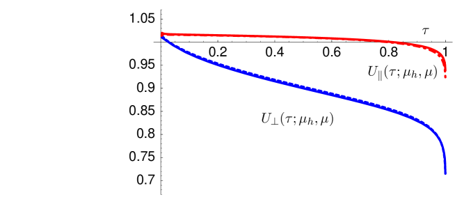
Figure 3: $U_{a}(\tau,\mu_{h},\mu)$ for $\mu_{h}=m_{b}=4.8$ GeV and $\mu=1.5$ GeV. The upper curves refer to $U_{\parallel}$, the lower ones to $U_{\perp}$. Solid lines: exact numerical integration. Dashed lines: approximate solutions.

4.2.2 NLO+LL approximation

We are now in the position to give expressions for the B-type short-distance coefficients $C(E,\tau;\mu)$, which include the complete 1-loop correction as well as the leading-logarithmic terms. The formula is

$$C(E,\tau;\mu) = C^{(0)}(E)+C^{(1)}(E,\tau;\mu)-C^{(0)}(E)\left[e^{-S}\,U_{a}\right]_{\alpha_{s}}\!(E,\tau;\mu)$$ (115)

$$+\,C^{(0)}(E)\left[e^{-S}\,U_{a}-1\right](E,\tau;\mu).$$

The meaning of the four terms on the right-hand side is as follows: the first and second terms are the tree and 1-loop coefficients, respectively. Together they constitute the next-to-leading order (NLO) approximation to $C(E,\tau;\mu)$. The fourth term is the sum of leading-logarithmic terms to all orders minus the tree. Finally, the third term subtracts the logarithmic terms already included in the full 1-loop correction $C^{(1)}(E,\tau;\mu)$. The subtraction is given by

$$\left[e^{-S}\,U_{a}\right]_{\alpha_{s}}\!(E,\tau;\mu) = \frac{\alpha_{s}(\mu)}{4\pi}\Bigg{\{}-\frac{\Gamma_{0}}{2}\left[\ln^{2}\left(\frac{\mu}{\mu_{h}}\right)+2\ln\left(\frac{\mu_{h}}{2E}\right)\ln\left(\frac{\mu}{\mu_{h}}\right)\right]$$ (116)

$$+\,\ln\left(\frac{\mu}{\mu_{h}}\right)\gamma_{a}(\tau)\Bigg{\}}$$

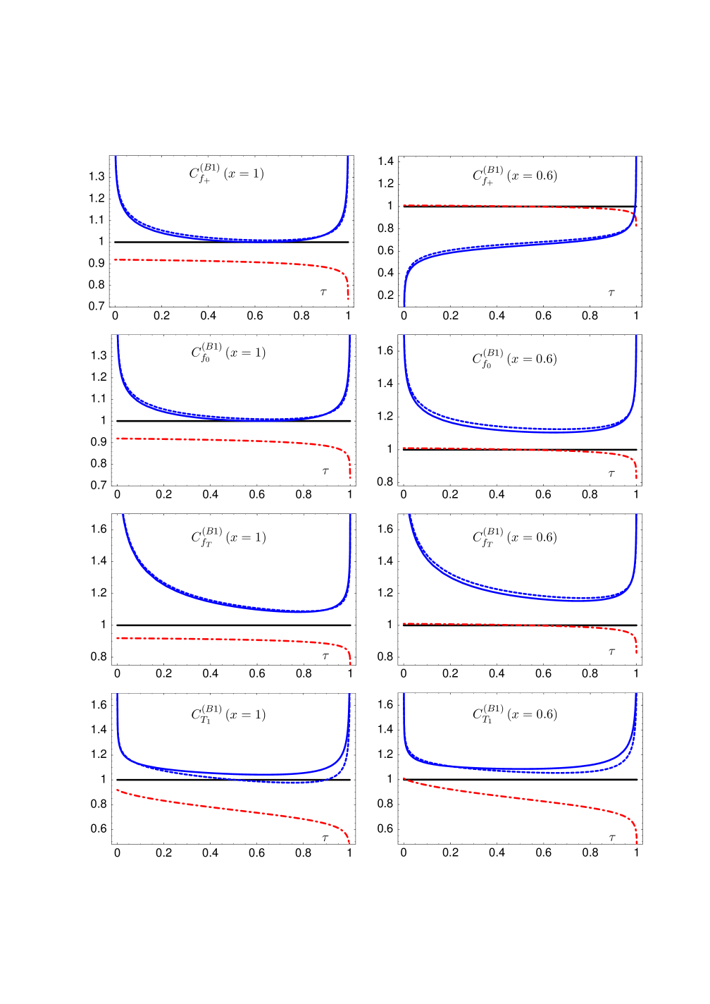
Figure 4: The short-distance coefficients $C^{(B1)}_{X}(E,\tau,\mu)$ relevant to the form factors $X$ at two representative energy values ($x=1$ (left) and $x=0.6$ (right)) at $\mu=1.5\,$GeV normalized to the tree approximation. Dash-dotted: logarithmic terms at order $\alpha_{s}$; dashed: full NLO approximation; solid: NLO plus logarithmic summation.

To analyze the structure of the correction, we display in Figure 4 the following approximations, all normalized to the tree coefficient: (i) tree plus the logarithmic terms at 1-loop (dash-dotted); (ii) previous approximation plus the non-logarithmic term, i.e. the complete next-to-leading order result (dashed); (iii) previous approximation plus the sum of leading-logarithmic terms at order $\alpha_{s}^{2}$ and beyond (solid). In the numerical implementation we set $\mu_{h}=m_{b}=4.8\,$GeV, $E=m_{b}x/2$, and regard the coefficients as functions of energy fraction $x$ and the convolution variable $\tau$. Since $E$ must be of order $m_{b}$, $x$ cannot be chosen too small. We take $x=1$ and $x=0.6$ as representative examples of large (maximal) and small energy of the light meson, and evolve to $\mu=1.5\,$GeV. We also fix the scale of the QCD tensor current operator to $\nu=m_{b}=4.8\,$GeV. Figure 4 shows four of the five combinations, $C^{(B1)}_{X}$, $X\in\{f_{+},f_{0},f_{T},T_{1},V\}$, which appear in the hard-scattering contribution to the vector and tensor current form factors (21), (22). Only $C^{(B1)}_{V}$ is not shown, because its tree coefficient vanishes, hence only $C^{(1)}(E,\tau;\mu)$ in (115) is non-zero.

The following observations can be made from the figure: a) the logarithmic term at order $\alpha_{s}$ (dash-dotted lines) is a very poor approximation to the full $\alpha_{s}$ coefficient (dashed lines), especially for $C^{(B1)}_{T_{1}}$, which is the only one of the four coefficients shown involving the transverse anomalous dimension $\gamma_{\perp}$. b) Except near the endpoints $\tau=0,1$, where the relative correction diverges, the typical next-to-leading order correction from the hard scale $m_{b}$ is of order 30%. The endpoint singularities are logarithmic and disappear when the correction is folded with the light-meson distribution amplitude (integration over $\tau$). c) The effect of the logarithmically enhanced terms beyond the order $\alpha_{s}$ is negligible (difference between the solid and dashed lines). It is largest for $C^{(B1)}_{T_{1}}$ towards larger $\tau$ since here $U_{\perp}(\tau;\mu_{h},\mu)$ is significantly different from 1, see Figure 3.

4.3 Spectator-scattering correction

According to (21), (22), (25) and (89) the form factors $F_{X}(E)$ are given by

$$F_{X}(E)=C^{(A0)}_{X}\,\xi_{a}(E)+H_{X}(E)$$ (117)

with the spectator-scattering term

$$H_{X}(E) = \frac{m_{B}}{4m_{b}}\,\hat{f}_{B}f_{M}\int_{0}^{1}dv\,\phi_{M}(v)\int_{0}^{\infty}d\omega\,\phi_{B+}(\omega)$$ (118)

$$\times\int_{0}^{1}d\tau\,C^{(B1)}_{X}(E,\tau)\,J_{a}(\tau;v,\omega).$$

Here $a=\,\parallel$ (or $P$ in case of $\xi_{a}$) for $X=\{f_{+},f_{0},f_{T}\}$ and $a=\,\perp$ for $X=\{V,T_{1}\}$. We have now assembled all the pieces required for the evaluation of $H_{X}(E)$ at order $\alpha_{s}^{2}$ (1-loop). From now on we set $m_{B}/m_{b}$ in (118) to 1, since the difference between the meson and the quark mass is a power correction beyond the accuracy of the present calculation.

At the leading order we insert the tree expressions for the B-type coefficient function (hereafter we again drop the superscript “B1”) and the jet-function and obtain

$$H_{X}^{(0)}(E)=-\frac{\pi\alpha_{s}(\mu)C_{F}}{N_{c}}\frac{\hat{f}_{B}f_{M}\langle\bar{v}^{-1}\rangle_{M}}{2E\lambda_{B}}\,C^{(0)}_{X}(E).$$ (119)

Here as before the superscript “(0)” refers to the tree approximation. This agrees with the results of [8].

To obtain the next-to-leading order result including the renormalization-group summation, we insert (115) and the jet-function into (118), and neglect cross terms of order $\alpha_{s}^{3}$ in the product $C_{X}\star J_{a}$. The result is

$$H_{X}(E) = H_{X}^{(0)}(E)\times\,\Bigg{\{}1+\frac{1}{\langle\bar{v}^{-1}\rangle_{M}}\int\frac{dv}{\bar{v}}\,\phi_{M}(v)\,\frac{C^{(1)}(E,\bar{v})}{C^{(0)}(E)}+\Big{[}I_{a}-1\Big{]}$$ (120)

$$-\,\frac{1}{\langle\bar{v}^{-1}\rangle_{M}}\int\frac{dv}{\bar{v}}\,\phi_{M}(v)\left[e^{-S}\,U_{a}\right]_{\alpha_{s}}(E,\bar{v})$$

$$+\frac{1}{\langle\bar{v}^{-1}\rangle_{M}}\int\frac{dv}{\bar{v}}\,\phi_{M}(v)\left[e^{-S}\,U_{a}-1\right](E,\bar{v})\Bigg{\}}.$$

The second term in the bracket is the 1-loop hard correction; the third comes from the jet-function and is defined in (99); the fourth and fifth are related to the renormalization group summation as in (115). The integration of the second term can be done analytically, but the expressions are lengthy. They are given for selected short-distance coefficients and for the integration with the asymptotic distribution amplitude in Appendix B. It is as straightforward to perform the integration over $\phi_{M}(v)$ numerically. The integration of the subtraction term is elementary and given by (116) together with (114). The integration of the last term can only be done numerically using the numerical solution of the integro-differential equation for $U_{a}$. Since $S$ is independent of $v$, one needs the integrals

$$\int_{0}^{1}\frac{dv}{\bar{v}}\,\phi_{M}(v,\mu)\,U_{\parallel}(\bar{v},\mu_{h},\mu) = 3.037+3.058\,a_{1}^{M}+3.051\,a_{2}^{M}+...\,,$$

$$\int_{0}^{1}\frac{dv}{\bar{v}}\,\phi_{M}(v,\mu)\,U_{\perp}(\bar{v},\mu_{h},\mu) = 2.795+2.980\,a_{1}^{M}+3.003\,a_{2}^{M}+...\,.$$ (121)

The numerical values are given for $\mu_{h}=4.8\,$GeV and $\mu=1.5\,$GeV.

To illustrate these results we consider the three coefficients relevant to the form factors in the physical form factor scheme defined in (25). Let

$$C_{0+}^{(B1)}(\tau,E) = C_{f_{0}}^{(B1)}(\tau,E)-C_{f_{+}}^{(B1)}(\tau,E)\,R_{0}(E),$$

$$C_{T+}^{(B1)}(\tau,E) = C_{f_{T}}^{(B1)}(\tau,E)-C_{f_{+}}^{(B1)}(\tau,E)\,R_{T}(E),$$

$$C_{T_{1}V}^{(B1)}(\tau,E) = C_{T_{1}}^{(B1)}(\tau,E)-C_{V}^{(B1)}(\tau,E)\,R_{\perp}(E).$$ (122)

Choosing $\lambda_{B}=0.35\,$GeV, $x=0.85$ (corresponding to light meson energy $E=xm_{B}/2=2.24\,$GeV or momentum transfer $q^{2}=4.18\,$GeV), and asymptotic distribution amplitudes, the curly bracket in (120) evaluates to

$$X=0+: \quad 1+0.283\mbox{ [C]}+0.371\mbox{ [jet]}+0.059\mbox{ [log, $\alpha_{s}$]}-0.073\mbox{ [all logs]},$$

$$X=T+: \quad 1+0.213\mbox{ [C]}+0.371\mbox{ [jet]}+0.059\mbox{ [log, $\alpha_{s}$]}-0.073\mbox{ [all logs]},$$

$$X=T_{1}V: \quad 1+0.209\mbox{ [C]}+0.268\mbox{ [jet]}+0.169\mbox{ [log, $\alpha_{s}$]}-0.147\mbox{ [all logs]},\phantom{--}$$ (123)

where the five terms correspond to the five terms on the right-hand side of (120). We observe that the hard correction [C] and the jet-function correction [jet] are of similar size, while the sum of higher-order logarithms (the sum of the last two terms) is at least a factor of 10 smaller. The total correction to the tree result amounts to an enhancement of (50-70)% of the spectator-scattering effect. These features are independent of the value of $E$ as can be seen from Figure 5, which displays the weak energy-dependence of the spectator-scattering correction normalized to the tree result.

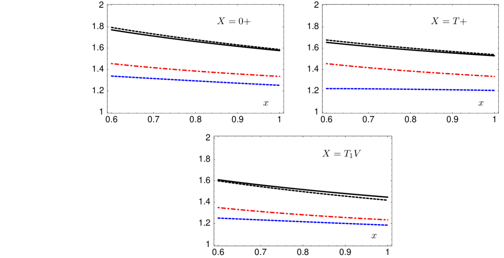
Figure 5: $H_{X}(E)/H_{X}^{(0)}(E)$ for $X=0+,T+,T_{1}V$. The two upper curves represent the complete next-to-leading order result with (solid) and without (dashed) the renormalization group summation. The middle (dash-dotted) line shows the jet-function (hard-collinear) correction alone, the lower (dashed) line the hard correction alone.

The dependence of these results on the hadronic input parameters $\lambda_{B}$, $a_{1}^{M}$, $a_{2}^{M}$ is roughly as follows. $\lambda_{B}$ enters the relative correction through the moments (98) and therefore affects the jet-function terms only. Choosing $\lambda_{B}=0.5\,$GeV ($0.25\,$GeV) changes the number 0.371 to 0.295 (0.452), and 0.268 to 0.195 (0.346), an uncertainty characteristic for all energy fractions $x$. Furthermore, there is an uncertainty due to the model for the shape of the distribution amplitude that correlates the logarithmic moments with $\lambda_{B}$, which we do not attempt to quantify. There is a larger dependence of the tree result $H_{X}^{(0)}(E)$ on $\lambda_{B}$, since it is inversely proportional to $\lambda_{B}$. Positive Gegenbauer moments increase the tree result and the relative next-to-leading order correction. This can be seen from (99) for the jet-function correction. For $a_{2}^{M}=0.2$, the total relative next-to-leading order correction increases from 64% for $X=+0$ (50% for $X=T_{1}V$) to 75% (62%). Finally, there is a dependence on the renormalization scale $\mu$, which we fixed to $1.5\,$GeV. In order to estimate this dependence, one must fix the hadronic input parameters at some $\mu_{0}$ and evolve them to $\mu$ using (93), (96). Since the scale-dependence of the hadronic parameters is within their uncertainty, we do not perform this estimate here.

5 B decay phenomenology

In this section we discuss three applications of our results to $B$ decays. We restrict ourselves to decays to pions or $\rho$ mesons, since the results for kaons are qualitatively very similar.

We use the following parameters: the $b$-quark pole mass $m_{b}=4.8\,$GeV; the renormalization scale of the QCD tensor current $\nu=m_{b}$; the initial scale for the renormalization group evolution $\mu_{h}=m_{b}$; the renormalization scale and final scale of the renormalization group evolution $\mu=1.5\,$GeV. This is also the (hard-collinear) scale at which all other scale-dependent quantities such as meson light-cone distribution amplitudes and the scale-dependent decays constants $\hat{f}_{B}$, $f_{M\perp}$ are evaluated. The strong coupling is obtained from $\alpha_{s}(m_{b})=0.215$ by employing 2-loop running ($\Lambda^{(n_{f}=4)}_{\overline{\rm MS}}=323.6\,$MeV), which gives $\alpha_{s}(1.5\,\mbox{GeV})=0.359$. The pion and $\rho$ meson parameters are $f_{\pi}=130.7\,\mbox{MeV}$, $f_{\rho\parallel}=209\,\mbox{MeV}$, $f_{\rho\perp}=150\,\mbox{MeV}$, and the second Gegenbauer moment is assumed to be $a_{2}^{M}=0.1$ for the pion and the distribution amplitudes of both, the longitudinal and transverse $\rho$ meson. The $B$ meson mass is $m_{B}=5.28\,$GeV and the decay constant $\hat{f}_{B}=f_{B}/K(1.5\,\mbox{GeV})=200\,$MeV. We assume the model (97) for the $B$ meson distribution amplitude and $\lambda_{B}=0.35\,$GeV. This is somewhat smaller than the value $0.46\,$GeV suggested by QCD sum rule calculations [34]. Allowing $\lambda_{B}$ to vary from $0.25\,$GeV to $0.5\,$GeV implies that the value of $\lambda_{B}$ is the single most important uncertainty in the final numerical calculation. The SCET_I form factors $\xi_{a}(E)$ are defined in the physical form factor scheme through full QCD form factors according to (24). The full QCD form factors needed for this definition are taken from the light-cone QCD sum rule calculations [35] including the parameterization of their $q^{2}$ dependence. On the basis of this input we can compute the remaining seven pion and $\rho$ meson form factors using (25). We relate hadronic to partonic variables by first eliminating $E$ through $E=xm_{b}/2$ in the coefficient functions. The energy fraction $x$ is then interpreted as $x=1-q^{2}/m_{B}^{2}=2E/m_{B}$, when we plot hadronic form factors as functions of $q^{2}$ or hadronic energy $E$.

5.1 Symmetry-breaking corrections to form factor ratios

In the absence of radiative and power corrections, the factorization formula (1) implies parameter-free relations between form factors [7], since only $\xi_{a}(E)$ appears on the right-hand side, which cancels in ratios. These relations receive corrections, which are calculable at leading power in the $1/m_{b}$ expansion given the above-mentioned input parameters [8]. The seven relations between the total of ten pion and $\rho$ meson form factors are obtained from the two relations (23), which do not receive any perturbative corrections, and the five relations that follow from (25) by dividing through the appropriate $\xi_{a}^{\rm FF}$. For instance, the second and third equations of (25) imply

$${\cal R}_{1}(E) \equiv \frac{m_{B}}{m_{B}+m_{P}}\frac{f_{T}(E)}{f_{+}(E)}=R_{T}(E)+\int_{0}^{1}d\tau\,C_{T+}^{(B1)}(\tau,E)\,\frac{\Xi_{P}(\tau,E)}{f_{+}(E)},$$

$${\cal R}_{2}(E) \equiv \frac{m_{B}+m_{V}}{m_{B}}\frac{T_{1}(E)}{V(E)}=R_{\perp}(E)+\frac{m_{B}+m_{V}}{m_{B}}\int_{0}^{1}d\tau\,C_{T_{1}V}^{(B1)}(\tau,E)\,\frac{\Xi_{\perp}(\tau,E)}{V(E)},\qquad$$ (124)

with $C_{T+}^{(B1)}(\tau,E)$, $C_{T_{1}V}^{(B1)}(\tau,E)$ the combinations of coefficient functions defined in (122). Similar relations follow for the other form factors. The second term on the right-hand side equals the hard spectator-scattering term (118) divided by the appropriate $\xi_{a}^{\rm FF}(E)$. Putting together (26), (119) and (120) we obtain the form factor ratios including the new next-to-leading order (and resummed) correction to the spectator-scattering term.

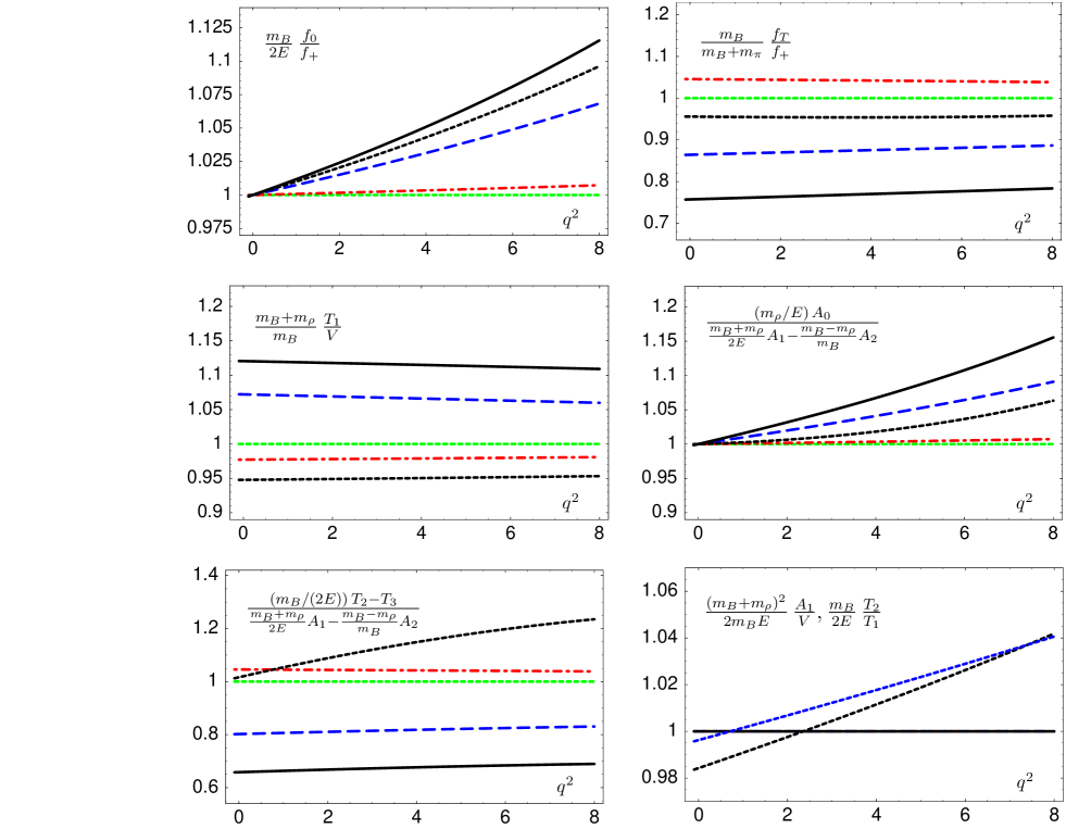
Figure 6: Corrections to the $B\to\pi$ and $B\to\rho$ form factor ratios as a function of $q^{2}$. The ratios equal 1 in the absence of radiative corrections. Solid (black) line: full result, including NLO and resummed leading-logarithmic correction to spectator-scattering; Long-dashed (blue): without NLO+LL correction to spectator-scattering; Dash-dotted (red): without any spectator-scattering term. Dashed (black): QCD sum rule calculation. The lower right panel shows the two form factor ratios that equal 1 at leading power. For comparison, the QCD sum rule results for these two ratios are shown (upper (blue) line refers to $A_{1}/V$, lower (black) line to $T_{2}/T_{1}$.)

The result of this computation is shown in Figure 6 for the various form factor ratios. The ratios are normalized such that in absence of any radiative corrections they equal 1 for all $q^{2}$. Our final result, which includes $R$ to order $\alpha_{s}$ and the spectator-scattering term to order $\alpha_{s}^{2}$ as well as the summation of leading logarithms to all orders is shown as the solid (black) curves. To display the size of the various contributions to the complete result, we also show the result following from neglecting the spectator-scattering term (dash-dotted (red) curves), and from evaluating the spectator-scattering contribution in leading-order (long-dashed (blue) curves), which corresponds to the previous results [8]. As has already been discussed in Section 4 the new NLO correction always enhances the symmetry-breaking effect. The correction from $R(E)$ in (124) is always smaller than the spectator-scattering contribution. In fact, it is even smaller than the NLO spectator-scattering term, despite the fact that the latter is formally of order $\alpha_{s}^{2}$. Overall, the deviations from the symmetry-limit range up to 40%, which is significant but not anomalously large given that the typical scales involved are in the range of $1.5\,$GeV. The theoretical uncertainties in the relative NLO spectator-scattering term have been discussed before in Section 4. The more important unknown factor resides in the normalization of the tree contribution (119), which involves the product

$$\frac{\hat{f}_{B}f_{M}\langle\bar{v}^{-1}\rangle_{M}}{\lambda_{B}\xi_{a}(E)}$$ (125)

of hadronic parameters. We estimate the theoretical errors of the factors to be around 15% ($\hat{f}_{B}$), 15% ($f_{\rho\perp}$), 10% ($\langle\bar{v}^{-1}\rangle_{M}$), 30% ($\lambda_{B}$) and 15% ($\xi_{a}(E)$), so it is clear that the curves in the figure are affected by a significant normalization uncertainty. In particular, adopting the QCD sum-rule result $\lambda_{B}=0.46\,$GeV rather than $0.35\,$GeV decreases the deviations of the form factor ratios from unity by about 30%.

It is instructive to compare this result for the form factor ratios with the QCD sum rule calculations. The corresponding sum rule ratios are shown as dashed (black; black and blue in the lower right panel) curves in Figure 6. One notices that the sum rule calculation satisfies the symmetry relations remarkably well – the ratios are in general closer to 1 than predicted on the basis of the heavy-quark limit corrected by radiative and spectator-scattering effects. There are also significant differences concerning the sign of the correction similar to those observed already in [8]. It is unclear whether the differences between the sum rule calculations and those based on the heavy-quark limit are due to $1/m_{b}$ power corrections or ununderstood systematics of the sum rule calculation (see the discussion in [36]). For instance, the sum-rule result for the ratio involving $m_{B}/(2E)\,T_{2}-T_{3}$ has changed from about 0.7 to almost 1.2 with the update [35] of the form factor calculations. This may not be surprising, since the ratio involves cancellations between form factors and may be particularly sensitive to the uncertainties of sum rule calculations. In such cases the SCET calculation of form factor relations is probably more reliable than the QCD sum rule method. In general, the comparison of the two methods leads to the conclusion that the theoretical calculations of form factors with QCD sum rules are affected by considerable uncertainties until the systematics of and discrepancies with the heavy-quark limit are better understood.

5.2 Radiative vs. semi-leptonic decay

Factorization calculations of radiative and hadronic two-body $B$ decays involving only light mesons (and leptons) make use of the form factors at maximal recoil. It is therefore of interest to investigate the short-distance corrections at $x=1$, i.e. $E=m_{B}/2$ or $q^{2}=0$. In addition to the exact relations (23), the first and fourth relations of (25) also degenerate to

$$\frac{m_{B}}{2E}\,f_{0}(E)=\xi_{P}^{\rm FF},\qquad\frac{m_{V}}{E}\,A_{0}(E)=\xi_{\parallel}^{\rm FF}$$ (126)

as a consequence of the equations of motion. This leaves only two interesting ratios, namely ${\cal R}_{1}$ and ${\cal R}_{2}$ defined in (124). The last ratio in (25) involving $T_{2}$ and $T_{3}$ can be obtained from ${\cal R}_{1}$ replacing $\xi_{P}^{\rm FF}=f_{+}$ by $\xi_{\parallel}^{\rm FF}$.

At $x=1$ we obtain the analytic expressions (assuming the asymptotic form $\phi_{M}(v)=6v\bar{v}$ for the light-meson distribution amplitude)

$${\cal R}_{1} = 1+\frac{\alpha_{s}}{4\pi}\left[-\frac{8}{3}\ln\frac{\nu}{m_{b}}+\frac{8}{3}\right]-\frac{8\pi\alpha_{s}(\mu)}{3}\,\frac{\hat{f}_{B}f_{M}}{M_{B}\lambda_{B}\xi_{P}^{\rm FF}}\,\Bigg{\{}1+\frac{\alpha_{s}(\mu)}{4\pi}$$

$$\times\,\Bigg{[}-\frac{8}{3}\ln\frac{\nu}{m_{b}}-\frac{8}{3}\ln^{2}\frac{m_{b}}{\mu}+\frac{4}{3}\left\langle\ln^{2}\frac{m_{b}\omega}{\mu^{2}}\right\rangle+\left(\frac{8}{3}-\frac{2\pi^{2}}{9}\right)\ln\frac{m_{b}}{\mu}$$

$$\hskip 19.91684pt+\,\left(-9+\frac{\pi^{2}}{9}+\frac{2n_{f}}{3}\right)\left\langle\ln\frac{m_{b}\omega}{\mu^{2}}\right\rangle+\frac{103}{6}+\frac{5\pi^{2}}{9}-\frac{19n_{f}}{9}+\delta_{\rm log}^{\parallel}\Bigg{]}\Bigg{\}}$$

$$= 1+0.046\,(R_{T})-0.165\,\Big{\{}1+0.540\,(\mbox{NLO spec.})-0.01\,(\delta_{\rm log}^{\parallel})\Big{\}}$$

$$= 0.794,$$

$${\cal R}_{2} = 1+\frac{\alpha_{s}}{4\pi}\left[-\frac{8}{3}\ln\frac{\nu}{m_{b}}-\frac{4}{3}\right]+\frac{4\pi\alpha_{s}(\mu)}{3}\,\frac{\hat{f}_{B}f_{M\perp}}{M_{B}\lambda_{B}\xi_{\perp}^{\rm FF}}\,\Bigg{\{}1+\frac{\alpha_{s}(\mu)}{4\pi}$$ (127)

$$\times\,\Bigg{[}-\frac{8}{3}\ln\frac{\nu}{m_{b}}-\frac{8}{3}\ln^{2}\frac{m_{b}}{\mu}+\frac{4}{3}\left\langle\ln^{2}\frac{m_{b}\omega}{\mu^{2}}\right\rangle+\left(-\frac{2}{3}-\frac{2\pi^{2}}{9}\right)\ln\frac{m_{b}}{\mu}$$

$$\hskip 19.91684pt+\,\left(-\frac{26}{3}+\frac{\pi^{2}}{9}+\frac{2n_{f}}{3}\right)\left\langle\ln\frac{m_{b}\omega}{\mu^{2}}\right\rangle+\frac{27}{2}+\pi^{2}-\frac{2\zeta(3)}{3}-\frac{19n_{f}}{9}+\delta_{\rm log}^{\perp}\Bigg{]}\Bigg{\}}$$

$$= 1-0.023\,(R_{T})+0.086\,\Big{\{}1+0.418\,(\mbox{NLO spec.})+0.03\,(\delta_{\rm log}^{\parallel})\Big{\}}$$

$$= 1.102,$$

where $\delta^{a}_{\rm log}$ denotes the small effect form the renormalization-group summation. The numerical results refer to the pion (${\cal R}_{1}$) and $\rho$ meson (${\cal R}_{2}$) with the parameters as specified above. The ratio ${\cal R}_{1}$ with $\xi_{P}^{\rm FF}=f_{+}$ replaced by $\xi_{\parallel}^{\rm FF}$ and pion parameters replaced by $\rho$ meson parameters gives 0.707 instead of 0.794. For comparison the QCD sum rule calculation [35] gives ${\cal R}_{1}=0.96$ (1.02 for $\rho$ and the relation involving $T_{2}$, $T_{3}$) and ${\cal R}_{2}=0.95$.

The factorization approach allows us to make predictions for the exclusive radiative $B$ decays $B\to M\gamma$ [2, 37] and $B\to Ml^{+}l^{-}$ [38]. The decays $B\to\rho\gamma$ together with $B\to K^{*}\gamma$ are particularly interesting, because they may lead to a determination of the CKM matrix element $|V_{td}|$ or constrain flavour non-universality in penguin transitions. The main limitation turns out to be the poor knowledge of SU(3) flavour symmetry breaking in the ratio of tensor form factors $T_{1}^{\rho}(0)/T_{1}^{K^{*}}(0)$ [39, 40]. In [39] it was therefore suggested to take the ratio of the $B\to\rho\gamma$ to the differential semi-leptonic $B\to\rho l\nu$ branching fraction, which avoids the problem of SU(3)-breaking, but introduces the ratio $T_{1}/V$ of $\rho$-meson form factors at $q^{2}=0$. The method relies on normalizing the $B\to\rho\gamma$ rate to the differential decay rate

$$\frac{d^{2}\Gamma(B\to\rho l\nu)}{dq^{2}d\cos\theta}\propto(1+\cos\theta)^{2}\,H_{-}^{2}+(1-\cos\theta)^{2}\,(H_{+}^{2}+2H_{0}^{2})$$ (128)

near $\cos\theta=1$ (with $\theta$ the angle between the neutrino momentum and the $B$ meson momentum in the $l\nu$ center-of-mass frame) and $q^{2}=0$. The angle cut has the effect of isolating the negative helicity form factor $H_{-}$, which has a simple expression in the heavy-quark limit. Neglecting quadratic effects in the light meson mass,

$$H_{-}(q^{2}) = \sqrt{\frac{q^{2}}{m_{B}^{2}}}\left(\frac{m_{B}+m_{\rho}}{m_{B}}\,A_{1}(q^{2})+\frac{m_{B}^{2}-q^{2}}{m_{B}(m_{B}+m_{\rho})}\,V(q^{2})\right)$$ (129)

$$= 2\,\sqrt{\frac{q^{2}}{m_{B}^{2}}}\left(1-\frac{q^{2}}{m_{B}^{2}}\right)\,\frac{m_{B}}{m_{B}+m_{\rho}}\,V(q^{2}),$$

hence the ratio of branching fractions involves

$$\frac{H_{-}^{2}}{T_{1}^{2}}=\frac{4q^{2}}{m_{B}^{2}}\left(1-\frac{q^{2}}{m_{B}^{2}}\right)^{\!2}\frac{H_{-}^{2}}{{\xi_{\perp}^{\rm FF}}^{2}}\,\,\stackrel{{\scriptstyle q^{2}\to 0}}{{\to}}\,\,\frac{4q^{2}}{m_{B}^{2}}\,\frac{1}{{\cal R}_{2}^{2}}.$$ (130)

Assigning a 60% uncertainty to the spectator-scattering contribution to ${\cal R}_{2}$ we obtain $1/{\cal R}_{2}^{2}=0.82\pm 0.12$ to be compared with the QCD sum rule value $1/{\cal R}_{2}^{2}=1.11\pm 0.22$, where we assigned a 10% uncertainty to the calculation of [35]. The disagreement between the two numbers is unfortunate and should be resolved. Assuming the result of the calculation in the factorization approach, we obtain a 10% uncertainty on $|V_{td}/V_{ub}|$ from the form factor ratio in the method proposed in [39]. This does not include an uncertainty from power-suppressed effects.

The tensor-to-vector ratio ${\cal R}_{2}(q^{2})$ also appears in the forward-backward asymmetry in the electroweak penguin decays $B\to Ml^{+}l^{-}$. The complete calculation of the decay matrix element divides into “factorizable” and “non-factorizable” contributions [8, 38]. In this terminology, “factorizable” contributions are related to the heavy-to-light form factors, and hence are the relevant ones here. Inserting

$$(m_{B}+m_{V})\,\frac{T_{1}}{V}=(m_{B}-m_{V})\,\frac{T_{2}}{A_{1}}=m_{B}{\cal R}_{2}$$ (131)

into Eq. (75) of [38], we obtain the differential forward-backward asymmetry [8]

$$\frac{dA_{\rm FB}}{dq^{2}}\propto\mbox{Re}\,\Big{[}C_{9}+Y(q^{2})+\frac{2m_{b}M_{B}}{q^{2}}\,C_{7}^{\rm eff}\,{\cal R}_{2}(q^{2})+\mbox{non-fact. terms}\Big{]}.$$ (132)

Since the dependence on $q^{2}$ is mainly through ${\cal R}_{2}(q^{2})/q^{2}$ it follows that the increase of ${\cal R}_{2}(q^{2})$ by several percent due to the next-to-leading order spectator-scattering correction implies an increase in the position of the asymmetry zero in approximately the same proportion.

5.3 Hadronic decays

The jet-function computed in this paper also appears in the next-to-leading order correction to spectator-scattering in hadronic two-body $B$ decays to light mesons. We outline this effect by the example of $B\to\pi\pi$ decays, keeping the discussion short, since the NLO correction is not yet completely available.

The factorization formula reads [1]

$$\langle\pi\pi|Q_{i}|\bar{B}\rangle = f_{+}(0)\,\,T_{i}^{I}*f_{\pi}\phi_{\pi}+T_{i}^{II}*f_{B}\phi_{B+}*f_{\pi}\phi_{\pi}*f_{\pi}\phi_{\pi},$$ (133)

where $Q_{i}$ denotes an operator from the effective weak Hamiltonian, and the formula holds up to power corrections. The second term describes spectator-scattering. Its short-distance coefficient is a convolution $T_{i}^{II}=C_{i}^{II}\star J_{\parallel}$, where $C_{i}^{II}$ is the coefficient function of a generalization of a B-type operator that takes into account the second pion. Since the pion that does not pick up the spectator anti-quark from the $\bar{B}$ meson decouples at the hard-scale, the physics at the hard-collinear scale is exactly the same as in the $B\to\pi$ transition. Hence the jet-function in hadronic decays equals $J_{\parallel}$ [21], which has been computed above. Note that this implies that the strong rescattering phases are all generated at the hard scale $m_{b}$ (at leading order in the heavy-quark expansion), since the jet-function is real.

Spectator-scattering is particularly important for decay amplitudes of the “colour-suppressed” final state $\pi^{0}\pi^{0}$, because the colour-suppression is absent for the spectator-scattering term. The situation is opposite for the colour-allowed final state $\pi^{-}\pi^{+}$. Both amplitudes are relevant to $\pi^{-}\pi^{0}$. In the following we shall therefore focus on the coefficient $\alpha_{2}(\pi\pi)$ that describes the colour-suppressed tree amplitude. We emphasize that a complete NLO calculation of spectator-scattering requires the calculation of the hard coefficient $C_{i}^{II}$ as well. The remarks below must therefore be understood as preliminary.

Following the notation of [41] (Eqs. (35) and (47)) we write

$$\alpha_{2}(\pi\pi) = C_{2}+\frac{C_{1}}{N_{c}}+\frac{C_{1}}{N_{c}}\,\frac{\alpha_{s}(\mu)C_{F}}{4\pi}\,V_{2}(\pi)$$ (134)

$$+\,\frac{C_{1}}{N_{c}}\,\frac{\pi\alpha_{s}(\mu_{h})C_{F}}{N_{c}}\,\Big{[}H_{2}^{\rm tw2}(\pi\pi)\,I_{\parallel}+H_{2}^{\rm tw3}(\pi\pi)\Big{]},$$

where now $\mu$ should be chosen of order $m_{b}$ and $\mu_{h}$ is a hard-collinear scale assumed to be $\mu_{h}=\sqrt{\Lambda_{h}\mu}$ with $\Lambda_{h}=0.5\,\mbox{GeV}$. The $C_{i}$ are Wilson coefficients from the effective weak-interaction Hamiltonian, $V_{2}(\pi)$ is a vertex correction, and $H_{2}^{\rm tw2}(\pi\pi)+H_{2}^{\rm tw3}(\pi\pi)$ the spectator-scattering term at tree level, which we separated into a leading-power (“tw2”) and a power-suppressed “chirally enhanced” (“tw3”) term. The new ingredient in this formula is the factor $I_{\parallel}$, which equals 1 in the absence of the NLO correction to the jet-function, and is given by (99) including the correction. Exactly the same modification applies to the spectator-scattering contribution to $\alpha_{1}(\pi\pi)$ and the leading-power pieces of the penguin amplitudes. Numerically, with parameters defined in [41], we obtain

$$\alpha_{2}(\pi\pi) = 0.17-[0.17+0.08i\,]_{V_{2}}+\left\{\begin{array}[]{lc}[0.11\cdot 1.37]_{H_{2}^{\rm tw2}\,\cdot I_{\parallel}}+[0.07]_{H_{2}^{\rm tw3}}&\qquad\mbox{(default)}\\ {[0.29\cdot 1.57]}_{H_{2}^{\rm tw2}\,\cdot I_{\parallel}}+{[0.17]}_{H_{2}^{\rm tw3}}&\qquad\mbox{(S4)}\end{array}\right.$$ (137)

$$= \left\{\begin{array}[]{lc}0.22\,(0.18)-0.08i&\qquad\mbox{(default)}\\ 0.64\,(0.47)-0.08i&\qquad\mbox{(S4)}\end{array}\right.$$ (140)

The various terms and factors correspond to those in (134) and we show the numbers for the default parameter set and the set S4 that provides a better overall description of hadronic two-body modes. Due to the near cancellation of the tree term with the vertex correction the colour-suppressed tree amplitude comes essentially from spectator-scattering. The factors 1.37 and 1.57 show the effect from the NLO correction to the jet-function. In the final line the number in brackets gives the result from [41], the unbracketed number corresponds to including the new jet-function term. To illustrate the implications of these results, we show in Table 1 the CP-averaged $B\to\pi\pi$ branching fractions corresponding to the four cases (default vs. S4, with and without NLO jet-function correction). For simplicity, we only consider the NLO jet function correction to the tree amplitudes $\alpha_{1}(\pi\pi)$ and $\alpha_{2}(\pi\pi)$ (colour-allowed and colour-suppressed), but not to the penguin amplitudes, since this gives the dominant effect (and the results are preliminary anyway, see above). It is clearly seen that the NLO correction to spectator-scattering can have a significant effect. The enhancement of the colour-suppressed tree amplitude brings the theoretical computation in better agreement with data, since the large $\pi^{0}\pi^{0}$ rate and the small $\pi^{+}\pi^{-}$ to $\pi^{-}\pi^{0}$ ratio favour a large colour-suppressed tree amplitude [41]. We do not discuss the direct CP asymmetries, since we expect the still missing NLO hard correction to spectator-scattering (which includes a new source of rescattering phases) to be the more important factor.

Scenario	default, LO jet	default, NLO jet	S4, LO jet	S4, NLO jet
$\alpha_{1}(\pi\pi)$	$0.99+0.02i$	$0.98+0.02i$	$0.88+0.02i$	$0.81+0.02i$
$\alpha_{2}(\pi\pi)$	$0.18-0.08i$	$0.22-0.08i$	$0.47-0.08i$	$0.64-0.08i$
$\mbox{Br}(\bar{B}^{0}\to\pi^{+}\pi^{-})$	$8.86$	$8.62$	$5.17$	$4.58$
$\mbox{Br}(\bar{B}^{0}\to\pi^{0}\pi^{0})$	$0.35$	$0.40$	$0.70$	$1.13$
$\mbox{Br}(B^{-}\to\pi^{-}\pi^{0})$	$6.03$	$6.28$	$5.07$	$5.87$

Table 1: Tree amplitude coefficients $\alpha_{1}$ and $\alpha_{2}$, and the CP-averaged $\pi\pi$ branching ratios in units of $10^{-6}$ in the default and S4 scenario of [41] showing the effect of the NLO jet function correction.

6 Conclusion

Spectator-scattering plays an important role in the theory of exclusive $B$ decays. It is also rather complicated, because several scales, $m_{b}$ (hard), $\sqrt{m_{b}\Lambda}$ (hard-collinear), and $\Lambda$ (hadronic) are involved. The development of QCD factorization and soft-collinear effective theory has made it possible to formulate the calculation in terms of two separate matching steps, in which the effects from the short-distance scales $m_{b}$ and $\sqrt{m_{b}\Lambda}$ are calculated in perturbation theory. In previous work [18] we began the calculation of 1-loop corrections to spectator-scattering effects in heavy-to-light meson form factors in the large-recoil region with the computation of the hard coefficient functions. In this paper we have completed the second step with the computation of the hard-collinear coefficient function, also called jet-function. Since the calculation involves the definition of various renormalized operators in QCD, SCET_I, and SCET_II, and the treatment of evanescent operators in dimensional regularization, we have described the technical aspects of this work in some length. Our results provide a check of similar results obtained by Becher et al. [19, 20]. The jet-function computed here is relevant to many different $B$ decays, including radiative and hadronic $B$ decays in the QCD factorization approach.

The results may be summarized as follows: we find significant enhancements of spectator-scattering at next-to-leading order, which increase the deviation of form factor ratios from the asymptotic heavy quark limit, in which perturbative and power corrections are neglected. We have also included the summation of formally large logarithms $\ln m_{b}/\Lambda$, but found this effect to be negligible compared to the full 1-loop correction. Despite the small scale of order $1.5\,$GeV involved, there is no sign that a perturbative treatment is not applicable. The 1-loop effects from the hard scale and the hard-collinear scale are about equally important, being on the order of (20-40)% (depending on parameters), at least in the $\overline{\rm MS}$ factorization scheme adopted throughout this work. It follows that the dominant theoretical uncertainties are related to hadronic input parameters such as moments of light-cone distribution amplitudes and decay constants. In addition to the symmetry-breaking corrections to form factor ratios, we also discussed radiative and hadronic two-body decays. Although the jet-function constitutes only one aspect of the NLO correction to spectator-scattering in hadronic decays, we have seen that the NLO enhancement has interesting implications for final states with significant colour-suppressed tree amplitudes.

We would also like to emphasize the theoretical conclusions from this calculation, since the form factors are up to now the only observables, for which a complete two-step matching in soft-collinear effective theory has been explicitly carried out to the 1-loop level in a case with spectator-scattering. The factorization arguments that lead to the formula (1) rely on the demonstration that the B-type SCET_I currents can be matched to SCET_II without encountering endpoint-divergent convolution integrals, which would violate naive SCET_II factorization [12, 13]. The calculations performed here and in [18] provide an explicit verification of these arguments at the 1-loop level.

Note added: We have been informed of related work by G. Kirillin, in which he computes the 1-loop correction to the jet-function $J_{\parallel}$, and to the coefficient function $C^{(B1)}_{f_{+}}$.

Acknowledgements

We are grateful to S. Jäger for careful reading of the manuscript. M.B. would like to thank the INT, Seattle and KITP, Santa Barbara for their generous hospitality during the summer of 2004, when most of this work was being done. D.Y. acknowledges support from the Alexander-von-Humboldt Stiftung and the Japan Society for the Promotion of Science. The work of M.B. is supported in part by the DFG Sonderforschungsbereich/Transregio 9 “Computergestützte Theoretische Teilchenphysik”.

Appendix A Short-distance coefficients

A.1 Change of basis

The coefficient functions of the operators defined in (• ‣ 2.1) to (• ‣ 2.1) are given in terms of those defined and calculated in [18] (denoted with subscript “old”) as follows:

$$\mbox{scalar}:$$

$$C_{S}^{(A0)} = C_{S\rm{\rm old}}^{(A0)},$$

$$C_{S}^{(B1)} = C_{S{\rm old}}^{(B1)}-\frac{C_{S{\rm old}}^{(A0)}}{x}\,,$$ (141)

$$\mbox{vector}:$$

$$C_{V}^{(A0)1} = C_{V\rm{\rm old}}^{(A0)1}\,,\hskip 56.9055ptC_{V}^{(A0)2}\,=\,C_{V\rm{\rm old}}^{(A0)3}\,,$$

$$C_{V}^{(A0)3} = C_{V\rm{\rm old}}^{(A0)2}-C_{V\rm{\rm old}}^{(A0)1}\,,$$

$$C_{V}^{(B1)1} = C_{V{\rm old}}^{(B1)3}-\frac{1}{x}\left(2C_{V{\rm old}}^{(A0)1}+C_{V{\rm old}}^{(A0)3}\right)\,,$$

$$C_{V}^{(B1)2} = -C_{V{\rm old}}^{(B1)2}+\frac{1}{x}\left(2C_{V{\rm old}}^{(A0)1}-C_{V{\rm old}}^{(A0)2}\right)\,,$$

$$C_{V}^{(B1)3} = C_{V{\rm old}}^{(B1)1}+\frac{1}{2}\,C_{V{\rm old}}^{(B1)4}+\frac{C_{V{\rm old}}^{(A0)2}}{x}\,,$$

$$C_{V}^{(B1)4} = \frac{1}{2}\,C_{V{\rm old}}^{(B1)4}-\frac{1}{x}\left(C_{V{\rm old}}^{(A0)1}-C_{V{\rm old}}^{(A0)2}\right)\,,$$ (142)

$$\mbox{tensor}:$$

$$C_{T}^{(A0)1} = -\frac{1}{2}\,C_{T\rm{\rm old}}^{(A0)1}\,,\hskip 56.9055ptC_{T}^{(A0)2}\,=\,C_{T\rm{\rm old}}^{(A0)3}\,,$$

$$C_{T}^{(A0)3} = C_{T\rm{\rm old}}^{(A0)2}-C_{T\rm{\rm old}}^{(A0)1}\,,\hskip 28.45274ptC_{T}^{(A0)4}\,=\,C_{T\rm{\rm old}}^{(A0)1}+C_{T\rm{\rm old}}^{(A0)3}-C_{T\rm{\rm old}}^{(A0)4}\,,$$

$$C_{T}^{(B1)1} = C_{T{\rm old}}^{(B1)2}-\frac{1}{2}\,C_{T{\rm old}}^{(B1)6}+\frac{1}{x}\left(C_{T{\rm old}}^{(A0)1}+C_{T{\rm old}}^{(A0)4}\right)\,,$$

$$C_{T}^{(B1)2} = C_{T{\rm old}}^{(B1)1}-C_{T{\rm old}}^{(B1)5}-\frac{C_{T{\rm old}}^{(A0)1}}{x}\,,$$

$$C_{T}^{(B1)3} = -\frac{1}{2}\,C_{T{\rm old}}^{(B1)6}-\frac{1}{x}\left(C_{T{\rm old}}^{(A0)1}+C_{T{\rm old}}^{(A0)3}-C_{T{\rm old}}^{(A0)4}\right)\,,$$

$$C_{T}^{(B1)4} = -C_{T{\rm old}}^{(B1)5}+\frac{1}{x}\left(C_{T{\rm old}}^{(A0)1}-C_{T{\rm old}}^{(A0)2}\right)\,,$$

$$C_{T}^{(B1)5} = C_{T{\rm old}}^{(B1)3}-\frac{1}{x}\left(2C_{T{\rm old}}^{(A0)2}+2C_{T{\rm old}}^{(A0)3}-C_{T{\rm old}}^{(A0)4}\right)\,,$$

$$C_{T}^{(B1)6} = \frac{1}{2}\,C_{T{\rm old}}^{(B1)4}-\frac{1}{2x}\left(C_{T{\rm old}}^{(A0)1}-2C_{T{\rm old}}^{(A0)2}\right)\,,$$

$$C_{T}^{(B1)7} = \frac{1}{4}\left(C_{T{\rm old}}^{(B1)7}-C_{T{\rm old}}^{(B1)4}\right)+\frac{1}{2x}\left(C_{T{\rm old}}^{(A0)1}-C_{T{\rm old}}^{(A0)2}\right)\,.$$ (143)

In the new basis the pseudoscalar coefficients equal the scalar coefficients, and the axial-vector coefficients equal the vector coefficients. Furthermore $x=n_{-}v\,n_{+}p^{\prime}/m_{b}=2E/m_{b}$ with $E$ the energy of the light meson.

A.2 Coefficients appearing in the form factors

The five independent A0-coefficients appearing in the SCET_I representation of the form factors (21), (22) are given by

$$C^{(A0)}_{f_{+}} = C_{V}^{(A0)1}+\frac{x}{2}C_{V}^{(A0)2}+C_{V}^{(A0)3}$$

$$= 1+\frac{\alpha_{s}C_{F}}{4\pi}\bigg{[}-2\ln^{2}\bigg{(}\frac{x}{\hat{\mu}}\bigg{)}+5\ln\bigg{(}\frac{x}{\hat{\mu}}\bigg{)}-2{\rm Li}_{2}(1-x)-\frac{\pi^{2}}{12}-3\ln x-6\bigg{]}\,,$$

$$C^{(A0)}_{f_{0}} = C_{V}^{(A0)1}+\bigg{(}1-\frac{x}{2}\bigg{)}C_{V}^{(A0)2}+C_{V}^{(A0)3}$$

$$= 1+\frac{\alpha_{s}C_{F}}{4\pi}\bigg{[}-2\ln^{2}\bigg{(}\frac{x}{\hat{\mu}}\bigg{)}+5\ln\bigg{(}\frac{x}{\hat{\mu}}\bigg{)}-2{\rm Li}_{2}(1-x)-\frac{\pi^{2}}{12}-\frac{3-5x}{1-x}\ln x-4\bigg{]}\,,$$

$$C^{(A0)}_{f_{T}} = -2C_{T}^{(A0)1}+C_{T}^{(A0)2}-C_{T}^{(A0)4},$$ (144)

$$= 1+\frac{\alpha_{s}C_{F}}{4\pi}\bigg{[}-2\ln\hat{\nu}-2\ln^{2}\bigg{(}\frac{x}{\hat{\mu}}\bigg{)}+5\ln\bigg{(}\frac{x}{\hat{\mu}}\bigg{)}-2{\rm Li}_{2}(1-x)-\frac{\pi^{2}}{12}$$

$$-\frac{3-x}{1-x}\ln x-6\bigg{]}\,$$

$$C^{(A0)}_{V} = C^{(A0)1}_{V}$$

$$= 1+\frac{\alpha_{s}C_{F}}{4\pi}\bigg{[}-2\ln^{2}\bigg{(}\frac{x}{\hat{\mu}}\bigg{)}+5\ln\bigg{(}\frac{x}{\hat{\mu}}\bigg{)}-2{\rm Li}_{2}(1-x)-\frac{\pi^{2}}{12}-\frac{3-2x}{1-x}\ln x-6\bigg{]}\,,$$

$$C^{(A0)}_{T_{1}} = -2C_{T}^{(A0)1}+\bigg{(}1-\frac{x}{2}\bigg{)}C_{T}^{(A0)2}+C_{T}^{(A0)3}$$

$$= 1+\frac{\alpha_{s}C_{F}}{4\pi}\bigg{[}-2\ln\hat{\nu}-2\ln^{2}\bigg{(}\frac{x}{\hat{\mu}}\bigg{)}+5\ln\bigg{(}\frac{x}{\hat{\mu}}\bigg{)}-2{\rm Li}_{2}(1-x)-\frac{\pi^{2}}{12}-3\ln x-6\bigg{]}\,.$$

The variable $E$ used in (21), (22) is related to $x$ through $x=n_{-}v\,n_{+}p^{\prime}/m_{b}=2E/m_{b}$. We also define $\alpha_{s}=\alpha_{s}(\mu)$, $\hat{\mu}=\mu/m_{b}$ and $\hat{\nu}=\nu/m_{b}$, where $\nu$ is the renormalization scale of the QCD tensor current, and $\mu$ is the SCET_I renormalization scale. The $\mu$ dependence cancels the corresponding dependence of the SCET_I form factors $\xi_{a}(E)$. The heavy quark mass is renormalized in the pole scheme. The five independent B-coefficients are given by

$$C^{(B1)}_{f_{+}} = \frac{x}{2}C_{V}^{(B1)1}+C_{V}^{(B1)2}$$

$$= \bigg{(}{-2}+\frac{1}{x}\bigg{)}\Bigg{\{}1+\frac{\alpha_{s}C_{F}}{4\pi}\bigg{[}-2\ln^{2}\bigg{(}\frac{x}{\hat{\mu}}\bigg{)}+\ln\bigg{(}\frac{x}{\hat{\mu}}\bigg{)}-\frac{3}{1-2x}\ln x-2{\rm Li}_{2}(1-x)-\frac{\pi^{2}}{12}$$

$$-\frac{2(1-x)}{1-2x}+\frac{x}{(1-2x)(1-x\xi)}-\frac{4(1-x)}{(1-2x)\bar{\xi}}\ln\xi+\frac{x(2-x\xi)}{(1-2x)(1-x\xi)^{2}}\ln(x\xi)\bigg{]}$$

$$+\,\frac{\alpha_{s}}{4\pi}\bigg{(}C_{F}-\frac{C_{A}}{2}\bigg{)}\,\bigg{[}\frac{4}{\xi}\ln\bar{\xi}\ln\hat{\mu}+\frac{2}{\xi}F(x,x\bar{\xi})+\frac{2}{x(1-2x)\xi\bar{\xi}}G$$

$$+\frac{2}{1-2x}\bigg{(}\frac{2(1-x)}{\xi}\ln\bar{\xi}+\frac{3-2x}{\bar{\xi}}\ln\xi-\frac{x}{1-x\xi}\ln(x\xi)\bigg{)}\bigg{]}\Bigg{\}},$$

$$C^{(B1)}_{f_{0}} = \bigg{(}1-\frac{x}{2}\bigg{)}C_{V}^{(B1)1}+C_{V}^{(B1)2}$$

$$= -\frac{1}{x}\Bigg{\{}1+\frac{\alpha_{s}C_{F}}{4\pi}\bigg{[}-2\ln^{2}\bigg{(}\frac{x}{\hat{\mu}}\bigg{)}+\ln\bigg{(}\frac{x}{\hat{\mu}}\bigg{)}-3\ln x-2{\rm Li}_{2}(1-x)-\frac{\pi^{2}}{12}$$

$$+\frac{2}{\bar{\xi}}\bigg{(}\frac{(2-x)\ln x}{1-x}-\frac{(2-x\xi)\ln(x\xi)}{1-x\xi}\bigg{)}+\frac{x(2-x\xi)}{(1-x\xi)^{2}}\ln(x\xi)+\frac{x}{1-x\xi}\bigg{]}$$

$$+\,\frac{\alpha_{s}}{4\pi}\bigg{(}C_{F}-\frac{C_{A}}{2}\bigg{)}\,\bigg{[}\frac{4}{\xi}\ln\bar{\xi}\ln\hat{\mu}+\frac{2}{\bar{\xi}}\ln\xi-\frac{2x}{1-x\xi}\ln(x\xi)+\frac{2}{\xi}F(x,x\bar{\xi})-\frac{2}{x\xi\bar{\xi}}G\bigg{]}\Bigg{\}}\,,$$

$$C^{(B1)}_{f_{T}} = -C^{(B1)5}_{T}$$

$$= \frac{1}{x}\Bigg{\{}1+\frac{\alpha_{s}C_{F}}{4\pi}\bigg{[}-2\ln\hat{\nu}-2\ln^{2}\bigg{(}\frac{x}{\hat{\mu}}\bigg{)}+\ln\bigg{(}\frac{x}{\hat{\mu}}\bigg{)}-3\ln x-2{\rm Li}_{2}(1-x)-\frac{\pi^{2}}{12}-2$$

$$+\frac{2}{\bar{\xi}}\bigg{(}\frac{(2-x)\ln x}{1-x}-\frac{(2-x\xi)\ln(x\xi)}{1-x\xi}\bigg{)}-\frac{x(2-x\xi)\ln(x\xi)}{(1-x\xi)^{2}}-\frac{x}{1-x\xi}\bigg{]}$$

$$+\,\frac{\alpha_{s}}{4\pi}\bigg{(}C_{F}-\frac{C_{A}}{2}\bigg{)}\,\bigg{[}\frac{4}{\xi}\ln\bar{\xi}\ln\hat{\mu}+\frac{2}{\bar{\xi}}\ln\xi+\frac{2x}{1-x\xi}\ln(x\xi)+\,\frac{2}{\xi}F(x,x\bar{\xi})-\frac{2}{x\xi\bar{\xi}}G\bigg{]}\Bigg{\}}\,,$$

$$C^{(B1)}_{V} = C^{(B1)4}_{V}$$

$$= \frac{\alpha_{s}C_{F}}{4\pi}\frac{1}{1-x\xi}\bigg{[}\frac{x\ln x}{1-x}-\frac{\ln(x\xi)}{1-x\xi}-\frac{\ln\xi}{\bar{\xi}}-1\bigg{]}\$$

$$+\,\frac{\alpha_{s}}{4\pi}\bigg{(}C_{F}-\frac{C_{A}}{2}\bigg{)}\,\bigg{[}-\frac{2}{x\xi}\ln\bar{\xi}-\frac{2}{x\bar{\xi}}\ln\xi+\frac{2\ln(x\bar{\xi})}{1-x\bar{\xi}}+\frac{2\ln(x\xi)}{1-x\xi}-\frac{2}{x^{2}\xi\bar{\xi}}G\bigg{]}\,,$$

$$C^{(B1)}_{T_{1}} = \bigg{(}1-\frac{x}{2}\bigg{)}C^{(B1)3}_{T}+C^{(B1)4}_{T}$$ (145)

$$= (-1)\,\Bigg{\{}1+\frac{\alpha_{s}C_{F}}{4\pi}\bigg{[}-2\ln\hat{\nu}-2\ln^{2}\!\bigg{(}\frac{x}{\hat{\mu}}\bigg{)}+\ln\bigg{(}\frac{x}{\hat{\mu}}\bigg{)}+\ln x-2{\rm Li}_{2}(1-x)-\frac{\pi^{2}}{12}-1$$

$$-\frac{4\xi}{\bar{\xi}}\ln\xi\ln\hat{\mu}-\frac{2}{\bar{\xi}}\ln\xi-\frac{2\xi}{\bar{\xi}}F(x,x\xi)\bigg{]}$$

$$+\,\frac{\alpha_{s}}{4\pi}\bigg{(}C_{F}-\frac{C_{A}}{2}\bigg{)}\,\bigg{[}\bigg{(}\frac{4(1+\xi)}{\xi}\ln\bar{\xi}+\frac{4\xi}{\bar{\xi}}\ln\xi\bigg{)}\ln\hat{\mu}-2\ln\bar{\xi}+2\ln\xi$$

$$-2F(x\bar{\xi},x\xi)+\frac{2}{\xi}F(x,x\bar{\xi})+\frac{2}{\bar{\xi}}F(x,x\xi)-\frac{2}{x\bar{\xi}}G$$

$$-\,\frac{2}{x\xi}\bigg{(}{\rm Li}_{2}(1-x)-{\rm Li}_{2}(1-x\bar{\xi})\bigg{)}-2\bigg{]}\Bigg{\}}\,.$$

The variables $E$ and $\tau$ used in (21), (22) are related to $x$ and $\xi$ through $x=2E/m_{b}$ and $\xi=\tau$. Diagrammatically $\xi$ corresponds to $n_{+}p^{\prime}_{2}/n_{+}p^{\prime}$, the fractional longitudinal momentum carried by the transverse collinear gluon in the B-type current operator. We also use $\bar{\xi}\equiv 1-\xi$, and introduced the two abbreviations

$$F(y,z) \equiv \ln^{2}y-\ln y+{\rm Li}_{2}(1-y)-\ln^{2}z+\ln z-{\rm Li}_{2}(1-z),$$

$$G \equiv {\rm Li}_{2}(1-x)-{\rm Li}_{2}(1-x\bar{\xi})-{\rm Li}_{2}(1-x\xi)+\frac{\pi^{2}}{6}.$$ (146)

These results are obtained by taking the appropriate linear combinations of the coefficients given in [18]. The variables $(x_{1},x_{2})$ used there are related to $(x,\xi)$ by $x_{1}=x\bar{\xi}$ and $x_{2}=x\xi$ ($\xi\in[0,1]$).

Appendix B Integrals of coefficient functions

B.1 Integration of the jet-function

The integrals $\int_{0}^{1}d\tau\,j_{a}(\tau;v,\omega)$ of the jet-functions (78), (79) are given by

$$\int_{0}^{1}d\tau\,j_{\parallel}(\tau;v,\omega) = C_{F}L^{2}$$

$$+\,\left(C_{F}\left[-\frac{7}{3}+2\ln\bar{v}\right]+\left(C_{F}-\frac{C_{A}}{2}\right)\left[\frac{22}{3}+\frac{2\ln v}{\bar{v}}\right]+\frac{4}{3}\,n_{f}T_{f}\right)L$$

$$+\,C_{F}\left[\frac{53}{9}-\frac{\pi^{2}}{6}+\left(-\frac{4}{3}+\frac{1}{v}\right)\ln\bar{v}+\ln^{2}\bar{v}\right]$$

$$+\,\left(C_{F}-\frac{C_{A}}{2}\right)\Bigg{[}-\frac{170}{9}+\left(\frac{22}{3}-\frac{2}{v}\right)\ln\bar{v}+\,\frac{1}{\bar{v}}\,\Bigg{(}\frac{\pi^{2}}{3}-2\ln v+\ln^{2}v$$

$$+\,2(1-2v)\Big{(}\mbox{Li}_{2}(v)-\mbox{Li}_{2}(\bar{v})\Big{)}\Bigg{)}\Bigg{]}+\left(-\frac{5}{3}+\ln\bar{v}\right)\frac{4}{3}\,n_{f}T_{f},$$

$$\int_{0}^{1}d\tau\,j_{\perp}(\tau;v,\omega) = C_{F}L^{2}$$ (147)

$$+\,\left(C_{F}\left[-\frac{7}{3}+2\ln\bar{v}\right]+\left(C_{F}-\frac{C_{A}}{2}\right)\left[\frac{22}{3}+\frac{2\bar{v}}{v}\ln\bar{v}+\frac{2(2-v)\ln v}{\bar{v}}\right]+\frac{4}{3}\,n_{f}T_{f}\right)L$$

$$+\,C_{F}\left[\frac{44}{9}-\frac{\pi^{2}}{6}+\left(-\frac{7}{3}+\frac{2}{v}\right)\ln\bar{v}+\ln^{2}\bar{v}\right]$$

$$+\,\left(C_{F}-\frac{C_{A}}{2}\right)\Bigg{[}-\frac{152}{9}+\left(\frac{22}{3}-\frac{2}{v}\right)\ln\bar{v}+\frac{\bar{v}}{v}\ln^{2}\bar{v}+\,\frac{1}{v\bar{v}}\,\Bigg{(}\frac{\pi^{2}}{3}-2v\ln v$$

$$+\,v(2-v)\ln^{2}v+2(1-2v)\Big{(}\mbox{Li}_{2}(v)-\mbox{Li}_{2}(\bar{v})\Big{)}\Bigg{)}\Bigg{]}+\left(-\frac{5}{3}+\ln\bar{v}\right)\frac{4}{3}\,n_{f}T_{f}.$$

The analytic expressions of the integrals entering $I_{a}$ (see (90)) read (setting $n_{f}=4$, $T_{f}=1/2$ and $C_{F}=4/3$ and $C_{A}=3$)

$$\frac{\lambda_{B}}{3}\int_{0}^{1}\frac{dv}{\bar{v}}\,\phi_{M}(v)\int_{0}^{\infty}\frac{d\omega}{\omega}\,\phi_{B+}(\omega)\int_{0}^{1}d\tau j_{\parallel}(\tau;v,\omega)$$ (148)

$$= \frac{4}{3}\langle L^{2}\rangle+\left(-\frac{19}{3}+\frac{\pi^{2}}{9}\right)\langle L\rangle+\frac{169}{18}-\frac{2\pi^{2}}{9}-\frac{8}{3}\zeta(3)$$

$$+a_{1}^{M}\bigg{[}\frac{4}{3}\langle L^{2}\rangle+\left(-\frac{110}{9}+\frac{\pi^{2}}{3}\right)\langle L\rangle+\frac{464}{27}+\frac{\pi^{2}}{9}-8\zeta(3)\bigg{]}$$

$$+a_{2}^{M}\bigg{[}\frac{4}{3}\langle L^{2}\rangle+\left(-\frac{157}{9}+\frac{2\pi^{2}}{3}\right)\langle L\rangle+\frac{646}{27}+\frac{8\pi^{2}}{9}-16\zeta(3)\bigg{]},$$

$$\frac{\lambda_{B}}{3}\int_{0}^{1}\frac{dv}{\bar{v}}\,\phi_{M}(v)\int_{0}^{\infty}\frac{d\omega}{\omega}\,\phi_{B+}(\omega)\int_{0}^{1}d\tau j_{\perp}(\tau;v,\omega)$$

$$= \frac{4}{3}\langle L^{2}\rangle+\left(-6+\frac{\pi^{2}}{9}\right)\langle L\rangle+\frac{65}{9}-\frac{\pi^{2}}{3}-\frac{8}{3}\zeta(3)$$

$$+a_{1}^{M}\bigg{[}\frac{4}{3}\langle L^{2}\rangle+\left(-\frac{110}{9}+\frac{\pi^{2}}{3}\right)\langle L\rangle+\frac{413}{27}+\frac{\pi^{2}}{9}-8\zeta(3)\bigg{]}$$

$$+a_{2}^{M}\bigg{[}\frac{4}{3}\langle L^{2}\rangle+\left(-\frac{313}{18}+\frac{2\pi^{2}}{3}\right)\langle L\rangle+\frac{4975}{216}+\frac{7\pi^{2}}{9}-16\zeta(3)\bigg{]}.$$

B.2 Convolution of $C^{(B1)}_{X}$ with the light-cone distribution amplitude

Because the expressions are lengthy, we only list the results for the convolution of the three combinations of coefficients functions in the physical form factor scheme as defined in (25), and assume that the light-cone distribution amplitude are given by their asymptotic forms $\phi_{M}(v)=6v\bar{v}$. The convolution integrals read

$$\int_{0}^{1}\frac{dv}{\bar{v}}\,\phi_{M}(v)\left(C^{(B1)}_{f_{0}}-C^{(B1)}_{f_{+}}\,R_{0}\right)(x,\bar{v})$$

$$= -\frac{6(1-x)}{x}\,\Bigg{\{}1+\frac{\alpha_{s}C_{F}}{4\pi}\bigg{[}-2\ln^{2}\left(\frac{x}{\hat{\mu}}\right)+\ln\left(\frac{x}{\hat{\mu}}\right)-\left(2-\frac{1}{(1-x)^{2}}\right)\ln x$$

$$-\left(2+\frac{2}{x}\right){\rm Li}_{2}(1-x)-\frac{\pi^{2}}{12}\frac{x-4}{x}+6+\frac{x}{1-x}\bigg{]}$$

$$+\frac{\alpha_{s}}{4\pi}\left(C_{F}-\frac{C_{A}}{2}\right)\bigg{[}\left(\frac{4\pi^{2}}{3}-8\right)\ln\left(\frac{x}{\hat{\mu}}\right)-\frac{4x\ln x}{1-x}+4\ln x\,{\rm Li}_{2}(x)-4{\rm Li}_{3}(1-x)$$

$$-8{\rm Li}_{3}(x)+8-\frac{4\pi^{2}}{3}-4\zeta(3)\bigg{]}\Bigg{\}},$$

$$\int_{0}^{1}\frac{dv}{\bar{v}}\,\phi_{M}(v)\left(C^{(B1)}_{f_{T}}-C^{(B1)}_{f_{+}}\,R_{T}\right)(x,\bar{v})$$

$$= 6\,\Bigg{\{}1+\frac{\alpha_{s}C_{F}}{4\pi}\bigg{[}-2\ln\hat{\nu}-2\ln^{2}\left(\frac{x}{\hat{\mu}}\right)+\ln\left(\frac{x}{\hat{\mu}}\right)+\left(2+\frac{2}{x}+\frac{1}{1-x}\right)\ln x$$

$$-\left(2+\frac{2}{x}+\frac{2}{x^{2}}\right){\rm Li}_{2}(1-x)-\frac{\pi^{2}}{12}\frac{x^{2}-4x-4}{x^{2}}+3-\frac{2}{x}\bigg{]}$$

$$+\frac{\alpha_{s}}{4\pi}\left(C_{F}-\frac{C_{A}}{2}\right)\bigg{[}\left(\frac{4\pi^{2}}{3}-8\right)\ln\left(\frac{x}{\hat{\mu}}\right)+\frac{4+4x}{x}\ln x+4\ln x\,{\rm Li}_{2}(x)-\frac{4}{x^{2}}{\rm Li}_{2}(1-x)$$

$$-\left(4-\frac{4}{x^{2}}\right){\rm Li}_{3}(1-x)-8{\rm Li}_{3}(x)+8-\frac{4}{x}-\frac{2\pi^{2}}{3}\left(2-\frac{1}{x}-\frac{1}{x^{2}}\right)-\left(4+\frac{4}{x^{2}}\right)\zeta(3)\bigg{]}\Bigg{\}},$$

$$\int_{0}^{1}\frac{dv}{\bar{v}}\,\phi_{M}(v)\left(C^{(B1)}_{T_{1}}-C^{(B1)}_{V}\,R_{\perp}\right)(x,\bar{v})$$

$$= -3\,\Bigg{\{}1+\frac{\alpha_{s}C_{F}}{4\pi}\bigg{[}-2\ln\hat{\nu}-2\ln^{2}\left(\frac{x}{\hat{\mu}}\right)-\ln\left(\frac{x}{\hat{\mu}}\right)+\left(2+\frac{4}{x}+\frac{2}{1-x}\right)\ln x$$

$$-\left(2+\frac{2}{x}+\frac{4}{x^{2}}\right){\rm Li}_{2}(1-x)-\frac{\pi^{2}}{12}\frac{x^{2}-4x-8}{x^{2}}+\frac{9}{2}-\frac{4}{x}\bigg{]}$$

$$+\frac{\alpha_{s}}{4\pi}\left(C_{F}-\frac{C_{A}}{2}\right)\bigg{[}\left(\frac{4\pi^{2}}{3}-4\right)\ln\left(\frac{x}{\hat{\mu}}\right)+2\ln x-\frac{4(1-x)}{x}\ln x\,{\rm Li}_{2}(x)+\frac{4}{x}{\rm Li}_{2}(1-x)$$

$$-\left(4-\frac{4}{x}-\frac{4}{x^{2}}\right){\rm Li}_{3}(1-x)+\frac{8(1-x)}{x}{\rm Li}_{3}(x)+1-\frac{2\pi^{2}}{3}-4\left(1+\frac{1}{x}+\frac{1}{x^{2}}\right)\zeta(3)\bigg{]}\Bigg{\}}$$

with $x=2E/m_{b}$, $\hat{\mu}=\mu/m_{b}$, $\hat{\nu}=\nu/m_{b}$, and $\alpha_{s}=\alpha_{s}(\mu)$.

References

-
[1]
M. Beneke, G. Buchalla, M. Neubert, and C. T. Sachrajda,
Phys. Rev. Lett. 83 (1999) 1914 [hep-ph/9905312];
M. Beneke, G. Buchalla, M. Neubert and C. T. Sachrajda, Nucl. Phys. B 591 (2000) 313 [hep-ph/0006124]. -
[2]
M. Beneke, Th. Feldmann and D. Seidel,
Nucl. Phys. B 612 (2001) 25
[hep-ph/0106067];
S. W. Bosch and G. Buchalla, Nucl. Phys. B 621 (2002) 459 [hep-ph/0106081]. -
[3]
A. Abada et al.,
Nucl. Phys. B 416 (1994) 675
[hep-lat/9308007];
C. W. Bernard, P. Hsieh and A. Soni, Phys. Rev. Lett. 72 (1994) 1402 [hep-lat/9311010];
A. Abada et al., Nucl. Phys. Proc. Suppl. 119 (2003) 641 [hep-lat/0209092];
K. C. Bowler, J. F. Gill, C. M. Maynard and J. M. Flynn [UKQCD Collaboration], JHEP 0405 (2004) 035 [hep-lat/0402023];
J. Shigemitsu et al., [hep-lat/0408019];
M. Okamoto et al., Nucl. Phys. Proc. Suppl. 140 (2005) 461 [hep-lat/0409116]. -
[4]
V. L. Chernyak and I. R. Zhitnitsky,
Nucl. Phys. B 345 (1990) 137;
V. M. Belyaev, A. Khodjamirian and R. Rückl, Z. Phys. C 60 (1993) 349 [hep-ph/9305348];
A. Khodjamirian, R. Rückl, S. Weinzierl and O. I. Yakovlev, Phys. Lett. B 410 (1997) 275 [hep-ph/9706303];
E. Bagan, P. Ball and V. M. Braun, Phys. Lett. B 417 (1998) 154 [hep-ph/9709243];
P. Ball and V. M. Braun, Phys. Rev. D 58 (1998) 094016 [hep-ph/9805422];
P. Ball and R. Zwicky, Phys. Rev. D 71 (2005) 014015 [hep-ph/0406232];
P. Ball and R. Zwicky, Phys. Rev. D 71 (2005) 014029 [hep-ph/0412079]. -
[5]
M. Wirbel, B. Stech and M. Bauer,
Z. Phys. C 29 (1985) 637;
N. Isgur, D. Scora, B. Grinstein and M. B. Wise, Phys. Rev. D 39 (1989) 799;
D. Melikhov and B. Stech, Phys. Rev. D 62 (2000) 014006 [hep-ph/0001113]. - [6] N. Isgur and M. B. Wise, Phys. Lett. B 237 (1990) 527.
- [7] J. Charles, A. Le Yaouanc, L. Oliver, O. Pène, and J. C. Raynal, Phys. Rev. D 60 (1999) 014001 [hep-ph/9812358].
- [8] M. Beneke and Th. Feldmann, Nucl. Phys. B 592 (2001) 3 [hep-ph/0008255].
- [9] A. Szczepaniak, E. M. Henley and S. J. Brodsky, Phys. Lett. B 243 (1990) 287.
-
[10]
Y. Y. Keum, H. N. Li and A. I. Sanda,
Phys. Rev. D 63 (2001) 054008
[hep-ph/0004173];
C. D. Lü, K. Ukai and M. Z. Yang, Phys. Rev. D 63 (2001) 074009 [hep-ph/0004213]. - [11] S. Descotes-Genon and C. T. Sachrajda, Nucl. Phys. B 625 (2002) 239 [hep-ph/0109260].
-
[12]
M. Beneke and Th. Feldmann,
Nucl. Phys. B 685 (2004) 249
[hep-ph/0311335];
M. Beneke and Th. Feldmann, Eur. Phys. J. C 33 (2004) S241 [hep-ph/0308303]. - [13] B. O. Lange and M. Neubert, Nucl. Phys. B 690 (2004) 249 [hep-ph/0311345].
- [14] C. W. Bauer, D. Pirjol and I. W. Stewart, Phys. Rev. D 67 (2003) 071502 [hep-ph/0211069].
-
[15]
C. W. Bauer, S. Fleming, D. Pirjol, and I. W. Stewart,
Phys. Rev. D 63 (2001) 114020 [hep-ph/0011336];
C. W. Bauer, D. Pirjol, and I. W. Stewart, Phys. Rev. D 65 (2002) 054022 [hep-ph/0109045]. -
[16]
M. Beneke, A. P. Chapovsky, M. Diehl and Th. Feldmann,
Nucl. Phys. B 643 (2002) 431 [hep-ph/0206152];
M. Beneke and Th. Feldmann, Phys. Lett. B 553 (2003) 267 [hep-ph/0211358]. - [17] R. J. Hill and M. Neubert, Nucl. Phys. B 657 (2003) 229 [hep-ph/0211018].
- [18] M. Beneke, Y. Kiyo and D. s. Yang, Nucl. Phys. B 692 (2004) 232 [hep-ph/0402241].
- [19] T. Becher and R. J. Hill, JHEP 0410 (2004) 055 [hep-ph/0408344].
- [20] R. J. Hill, T. Becher, S. J. Lee and M. Neubert, JHEP 0407 (2004) 081 [hep-ph/0404217v2].
- [21] C. W. Bauer, D. Pirjol, I. Z. Rothstein and I. W. Stewart, Phys. Rev. D 70 (2004) 054015 [hep-ph/0401188].
- [22] D. Pirjol and I. W. Stewart, Phys. Rev. D 67 (2003) 094005 [Erratum-ibid. D 69 (2004) 019903] [hep-ph/0211251].
- [23] G. Burdman and G. Hiller, Phys. Rev. D 63 (2001) 113008 [hep-ph/0011266].
- [24] M. Beneke, Th. Feldmann and D. Seidel, Eur. Phys. J. C 41 (2005) 173 [hep-ph/0412400].
- [25] M. Beneke and V. A. Smirnov, Nucl. Phys. B 522 (1998) 321 [hep-ph/9711391].
-
[26]
V. A. Smirnov and E. R. Rakhmetov,
Theor. Math. Phys. 120 (1999) 870 [Teor. Mat. Fiz. 120 (1999) 64]
[hep-ph/9812529];
V. A. Smirnov, Applied Asymptotic Expansions In Momenta And Masses, Springer Verlag, Berlin, Germany, 2002. - [27] T. Becher, R. J. Hill and M. Neubert, Phys. Rev. D 69 (2004) 054017 [hep-ph/0308122].
-
[28]
G. P. Lepage and S. J. Brodsky,
Phys. Rev. D 22 (1980) 2157;
A. V. Efremov and A. V. Radyushkin, Phys. Lett. B 94 (1980) 245. - [29] B. O. Lange and M. Neubert, Phys. Rev. Lett. 91 (2003) 102001 [hep-ph/0303082].
- [30] X. D. Ji and M. J. Musolf, Phys. Lett. B 257 (1991) 409.
- [31] A. G. Grozin and M. Neubert, Phys. Rev. D 55, 272 (1997) [hep-ph/9607366].
- [32] M. Beneke, G. Buchalla, M. Neubert and C. T. Sachrajda, [hep-ph/0411171].
- [33] J. Kodaira and L. Trentadue, Phys. Lett. B 112 (1982) 66.
-
[34]
V. M. Braun, D. Y. Ivanov and G. P. Korchemsky,
Phys. Rev. D 69 (2004) 034014
[hep-ph/0309330];
A. Khodjamirian, T. Mannel and N. Offen, [hep-ph/0504091]. - [35] P. Ball and R. Zwicky, Ref. [4].
- [36] F. De Fazio, Th. Feldmann and T. Hurth, [hep-ph/0504088].
-
[37]
J. g. Chay and C. Kim,
Phys. Rev. D 68 (2003) 034013
[hep-ph/0305033];
S. Descotes-Genon and C. T. Sachrajda, Nucl. Phys. B 693 (2004) 103 [hep-ph/0403277];
T. Becher, R. J. Hill and M. Neubert, [hep-ph/0503263]. - [38] M. Beneke, Th. Feldmann and D. Seidel, Ref. [2].
- [39] S. W. Bosch and G. Buchalla, JHEP 0501 (2005) 035 [hep-ph/0408231].
-
[40]
A. Ali, E. Lunghi and A. Y. Parkhomenko,
Phys. Lett. B 595 (2004) 323
[hep-ph/0405075];
M. Beneke, T. Feldmann and D. Seidel, Ref. [24] -
[41]
M. Beneke and M. Neubert,
Nucl. Phys. B 675 (2003) 333
[hep-ph/0308039];
M. Beneke, G. Buchalla, M. Neubert and C. T. Sachrajda, Nucl. Phys. B 606 (2001) 245 [hep-ph/0104110].