Chemical thermalization in relativistic heavy ion collisions

Abstract

We compute by numerical integration of the Dirac equation the number of quark-antiquark pairs initially produced in the classical color fields of colliding ultrarelativistic nuclei. While the number of $q\bar{q}$ pairs is parametrically suppressed in the coupling constant, we find that in this classical field model their production rate is comparable to the thermal ratio of gluons/pairs = 9$N_{\mathrm{f}}$/32. After isotropization one thus would have a quark-gluon plasma in chemical equilibrium.

Much attention has recently been given to the thermalization properties of QCD matter formed in ultrarelativistic heavy ion collisions. Since 1983 bjorken hydrodynamic analysis have assumed rapid initial thermalization and essentially entropy conserving expansion thereafter. Now RHIC experiments phenixwhitepaper ; starwhitepaper strongly suggest that this is the correct picture. Theoretically, it is straightforward to understand the formation of an initial gluonic system, but the problem has been its isotropization in momentum space serreau . Weak coupling methods fail if they only include collective effects by screening mueller but show great promise if they include collective effects caused by the anisotropy of the system stantheman ; arnold ; strickland ; dumitrunara . However, this still leaves open the chemical equilibration of the system elliottrischke .

The physics involved here is as follows. Two large nuclei of radius $R_{A}$ moving along the light cone in opposite directions (Fig. 1) collide with zero impact parameter. They correspond to an ensemble of color currents moving along the light cone in opposite directions. The stochastic properties of the transverse color density $\rho^{a}(\mathbf{x}_{T})$ have been extensively studied iancuvenugopalan ; hatta . The magnitude of the charging is described by a parameter combination $g\mu$. For given element of the charge ensemble, color fields can be computed by solving the Yang-Mills equations $[D_{\mu},F^{\mu\nu}]=0$ with initial conditions given by continuity across the light cone kmw . For a dilute system (small $g^{2}\mu R_{A}$) one can compute the gluon fields analytically kmw ; kovchegovrischke . In general, the color fields can be obtained by a numerical computation krasnitzvenu ; lappi and then interpreted in terms of gluon production. The color fields are space and time dependent and a definite quantum mechanical probability of producing $q\bar{q}$ pairs is associated with them. These are pairs which are nonperturbatively produced during the first instants of the collision and which will contribute to chemical equilibration. We will compute their number and various distributions for numerically computed gluonic fields. Again, for weak fields this computation can be carried out analytically gelisvenu .

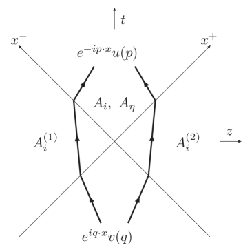
Figure 1: Domains of different time dependences. The fermion amplitude is a sum of two terms: one with interaction first with the left moving nucleus, then evolution over a region in which the gluon field $A_{i}^{(2)}$ is a gauge transform of the vacuum and finally evolution in a nontrivial gluon field $A_{i},A_{\eta}$. The other term is symmetric.

Assume now that the SU(3) color fields $A_{i}(\tau,\mathbf{x}_{T}),A_{\eta}(\tau,\mathbf{x}_{T})$ are known for $0\leq\tau\lesssim 1/Q_{\mathrm{s}}\approx 0.2\textrm{ fm}/c$ (RHIC value). A computation of pair production requires a careful discussion of in and out vacua and their relation. For the present field configuration this has been carried out in baltz . The computation, which is set up so that one obtains the average number of pairs, which is just the quantity we want, proceeds as follows. Choose an antiquark of momentum ${\bf q}$ and mass $m$ and solve as a function of time the Dirac equation with this color field for the spinor $\psi_{\bf q}(t,{\bf x})$ which in the distant past is given by the negative energy spinor $\psi_{\bf q}(t\to-\infty,{\bf x})=e^{iq\cdot x}v(q)$. The time integration brings in positive energy components and consists of three qualitatively different domains, see Fig. 1. The region $x^{\pm}<0$ is trivial. The regions marked $A_{i}^{(1)},A_{i}^{(2)}$ can be dealt with analytically 1+1d and one obtains an initial condition for $\psi_{\bf q}(\tau=0,z,\mathbf{x}_{T})$ along the positive light cones. This rather complicated initial condition, given explicitly in Eq. (16) of 1+1d , depends on the Wilson lines $U_{(1)}(\mathbf{x}_{T}),U_{(2)}(\mathbf{x}_{T})$ corresponding to the gauge fields of the nuclei, the initial color field $A_{i}(0,\mathbf{x}_{T})$ and on $y_{q},{\mathbf{q}_{T}},z,\mathbf{x}_{T}$. The spinor $\psi_{\bf q}(t,{\bf x})$ at $\tau>0$ is then computed by solving the Dirac equation in the given color field forward in time. Finally, one chooses a quark momentum ${\bf p}$ and forms the overlap between a positive energy spinor $\phi_{\bf p}(x)=e^{-ip\cdot x}u(p)$ and the outcome of the time evolution of the negative energy spinor in the distant past:

$$M_{\tau}(p,q)\equiv\int\frac{\tau\mathrm{d}z\mathrm{d}^{2}\mathbf{x}_{T}}{\sqrt{\tau^{2}+z^{2}}}\,\phi_{\bf p}^{\dagger}(\tau,{\bf x}){\gamma^{0}}\gamma^{\tau}\psi_{\bf q}(\tau,{\bf x})\;.$$ (1)

The overlap is computed at fixed $\tau$, hence the use of $\gamma^{\tau}$, ${\gamma^{0}}\gamma^{\tau}=\cosh\eta-{\gamma^{0}}{\gamma^{3}}\sinh\eta=\exp(-\eta{\gamma^{0}}{\gamma^{3}})$. This is also the reason for the Jacobian factor $\tau dz/\sqrt{\tau^{2}+z^{2}}$ in the longitudinal integration. We evaluate Eq. (1) in the 2-dimensional Coulomb gauge $\partial_{i}A_{i}=0$. This is the gauge condition used in the Abelian case baltz and also the one used to evaluate the number of gluons in the background field. Eq. (1) gives us

$${dN\over dy}=\int\frac{\mathrm{d}y_{p}\mathrm{d}^{2}{\mathbf{p}_{T}}}{2\left(2\pi\right)^{3}}\frac{\mathrm{d}y_{q}\mathrm{d}^{2}{\mathbf{q}_{T}}}{2\left(2\pi\right)^{3}}\delta\bigl{(}y-y_{p})\left|M_{\tau}(p,q)\right|^{2},$$ (2)

the number of quarks of one flavor of mass $m$ per unit rapidity (since an equal number of antiquarks are produced, we refer to this quantity as the “number of pairs” below). Since the gluon fields are $\eta$–independent, $dN/dy$ is independent of $y$. We shall compute (2) for all $\tau$ but it is only after the “formation time” $\tau\gtrsim 1/\sqrt{q_{T}^{2}+m^{2}}$ that the produced antiquarks can reinteract. Since one expects $q_{T}\sim g^{2}\mu$, this limit for light quarks is $\tau\gtrsim 1/(g^{2}\mu)$.

The parameters of the computation are the coupling $g$ (constant in this semiclassical set-up; we use the phenomenologically relevant value $g=2$, $\alpha_{s}=0.3$) the source density parameter $\mu$ (depends on atomic number $A$ and collision energy $\sqrt{s}$) the nuclear radius $R_{A}$ and the quark mass $m$ (like with $g$ there is nothing in this semiclassical set-up which would make $m$ scale dependent).

Two relevant parameter combinations are $g^{2}\mu$ and $g^{2}\mu R_{A}$. The first one, $g^{2}\mu$, is the dominant transverse momentum scale of the classical background field. It is related to the saturation scale $Q_{\mathrm{s}}$; for ${\mathbf{k}_{T}}<Q_{\mathrm{s}}$ the gluonic system becomes so dense that nonlinear interactions limit the growth of its density, numerically in one phenomenological model ekrt $Q_{\mathrm{s}}\approx 0.2\,{\rm GeV}A^{0.128}\sqrt{s}^{0.19}$, $Q_{\mathrm{s}}\approx 1$ GeV at RHIC energies and $\approx 2$ GeV at LHC energies. The dimensionless diluteness parameter $g^{2}\mu R_{A}$ determines the importance of nonlinear strong field effects.

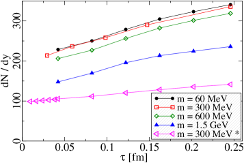
Figure 2: Dependence on proper time $\tau$ of the number of pairs per unit rapidity $\mathrm{d}N/\mathrm{d}y$ for $g^{2}\mu=2$ GeV and for values of quark mass marked on the figure. The lowest curve corresponds to $g^{2}\mu=1$ GeV.

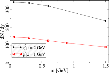
Figure 3: Dependence of the number of quark pairs on quark mass at a fixed proper time, $\tau=0.25\textrm{ fm}$, and for two values of $g^{2}\mu$.

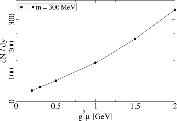
Figure 4: Dependence of the number of quark pairs on $g^{2}\mu$ at a fixed proper time, $\tau=0.25\textrm{ fm}$, and for quark mass $m=0.3\textrm{ GeV}$.

The numerical computation is done on a $N_{T}^{2}N_{L}$ lattice so that the total transverse area is $(N_{T}a)^{2}=\pi(6.7\,\textrm{ fm})^{2}$, i.e., the transverse lattice spacing is $a=11.8\,{\rm fm}/N_{T}=60/N_{T}\cdot 1/{\rm GeV}$. The results presented in this letter have been obtained with $N_{T}=180,\ N_{L}=400,\ \mathrm{d}z=0.2a$ and $\mathrm{d}\tau=0.02a$. At each site one has for each color a spinor with 4 complex components, i.e., ($N_{c}=3$)$\times 2\times 4\times 4=96$ bytes in single precision, giving a total of $96\cdot 180^{2}\cdot 400=1.2\textrm{ GB}$. This illustrates the memory requirement of the calculation. The number of timesteps in the integration in order to reach $\tau=0.25\textrm{ fm}$ is of the order of 500. The numerical method can be tested by varying these parameters. Another check of the numerical method is to study how for a zero external field the result of zero quark pairs is obtained in a rather nontrivial way by the contributions of the two paths in Fig.1 cancelling each other.

Note that on the transverse lattice one has to use lattice momenta

$$\tilde{k}^{2}={4\over a^{2}}\sum_{i=1}^{2}\sin^{2}{ak_{i}\over 2},\quad\hat{k}^{2}={1\over a^{2}}\sum_{i=1}^{2}\sin^{2}{ak_{i}},$$ (3)

for bosons and fermions, $ak_{i}=2\pi n_{i}/N_{T}$ with $-N_{T}/2+1<n_{i}\leq N_{T}/2$. For fermions the modes $N_{T}/4<|n_{i}|<N_{T}/2$ are doubler modes, which we leave out both from the initial condition ($q$ modes) and the projection to positive energy states ($p$ modes). For fermions one can effectively only go up to $\hat{k}=\sqrt{2}/a\approx\sqrt{2}N_{T}/60\textrm{ GeV}\approx 4\textrm{ GeV}$ on a $180^{2}$–lattice.

Results for the number of pairs are shown in Figs. 2–4. First, Fig. 2 shows how the pair production amplitude $M_{\tau}$ depends on proper time $\tau$ for $g^{2}\mu=2$ GeV and for a number of quark mass values, for $g^{2}\mu=1$ GeV the $\tau$ dependence for $m=0.3$ GeV is given. A striking feature of the result is the instantaneous formation of the pairs at small $\tau$, followed by gradual increase. To put this in perspective, note that in the QED case the production amplitude (1) can be computed analytically for all $\tau>0$ and its square is constant and equal to that of the pair production amplitude in baltz . In Abelian electrodynamics the production thus takes place instantaneously at $\tau=0$, Here there is also a slow increase thereafter and one will enter in a domain in which the backreaction of $q\bar{q}$ on the gluon fields should be included. In comparison, for $g^{2}\mu=2$ GeV the gluon number grows rapidly to the value $0.29\pi g^{2}\mu^{2}R_{A}^{2}\approx 1000$ by the time $1/g^{2}\mu\approx 0.1$ fm krasnitzvenu ; lappi and saturates thereafter.

The dependence of the result on quark mass $m$ and on $g^{2}\mu$ is shown in Figs. 3 and 4, both at $\tau=0.25$ fm. The dependence on the quark mass $m$ is surprisingly weak compared to the perturbative result. For numerical reasons we can not go down to quark masses $m\lesssim 100\textrm{ MeV}$. One should also note that with the small transverse lattice that we have used here one cannot study very large masses. The mass dependence is stronger for smaller $g^{2}\mu$, which is expected.

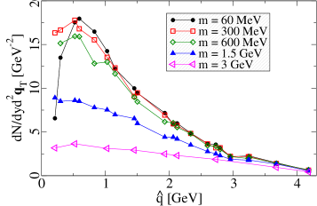
Figure 5: Transverse momentum spectrum of (anti)quarks for $g^{2}\mu=2$ GeV at a fixed proper time, $\tau=0.25$ fm, and for different quark masses.

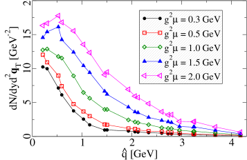
Figure 6: Transverse momentum spectrum of (anti)quarks for quark mass $m=0.3$ GeV and for different $g^{2}\mu$ at a fixed proper time, $\tau=0.25$ fm.

The computation of the gluon fields krasnitzvenu ; lappi is based on the Hamiltonian formalism and thus gives directly the transverse energy $E_{T}$. Obtaining the multiplicity is based on assuming free field dispersion relation. In the case of quarks, the pair multiplicity comes directly, and one must explicitly compute the transverse momentum spectra in order to obtain $E_{T}^{\mbox{\scriptsize pairs}}$. These are obtained from (2) by fixing $y_{q}=0$ and ${\mathbf{q}_{T}}$ and integrating over $y_{p},{\mathbf{p}_{T}}$. Results for various quark masses at fixed $g^{2}\mu=2$ GeV are shown in Fig. 5 and for various $g^{2}\mu$ at fixed $m=0.3$ GeV in Fig. 6.

One expects $q_{T}$-spectra to become flatter and smaller with increasing quark mass $m$ and flatter and larger with increasing $g^{2}\mu$. These qualitative features are seen in the result, but especially the mass dependence is rather weak.

It has conventionally been assumed that the initial state of a heavy ion collision is dominated by gluons. This is the result e.g. when both quarks and gluons are produced in $2\to 2$ collisions of collinear partons ekrt . In the color glass condensate picture the initial state is entirely gluonic and pair production is suppressed by a power of $g$. Our result suggests that quarks could be present in comparable numbers. This is understandable since the numerical value of the coupling constant $g$ is, in fact, not small. Note also that the kinematics are different: the calculation of gluon production in this approach reduces in the perturbative limit to a $2\to 1$ process, whereas the weak field limit of our present computation is a $2\to 2$ process. To be able to compare quark and gluon production to the same order in $g$ one must compute the first correction to the gluon production result, which has not yet been done in the color glass condensate picture. A first step in this direction is relaxing the assumption of boost invariance in solving the gauge field equations of motion rom .

The qualitative phenomenological implications of our result are as follows. Experiments at RHIC have observed about 600 charged ($\approx 1000$ charged and neutral) particles per unit rapidity. The assumption of entropy conservation, which is supported by the success of ideal hydrodynamics calculations, then implies as many particles per unit rapidity also in the initial state, which we are discussing. One has normally assumed that all the initial particles are gluons. In this framework, $g^{2}\mu=2$ GeV would lead to 1000 initial gluons. Now we see from Fig. 2 that, for 3 flavors, about 600 pairs would be produced. This implies that the initial assumption of gluon dominance should be questioned. In chemical thermal equilibrium the quark/gluon ratio is $9N_{\mathrm{f}}/32\approx 1$ meaning that 1000 particles in a unit of rapidity should consist of 330 gluons and 330 pairs. These numbers are obtained for $g^{2}\mu\approx 1.2$, i.e., the model gives a consistent fit with a reduced value of $g^{2}\mu$, smaller saturation scale.

There is now experimental evidence suggesting that QCD matter formed in ultrarelativistic heavy ion collisions is from the very beginning in local kinetic thermal equilibrium. This is what one always has assumed in applications of hydrodynamics, but its theoretical proof and understanding has been lacking as the process clearly is nonperturbative. We have in this letter shown that the classical gluon field model with an ensemble of initial conditions also produces an abundance of quark-antiquark pairs. In fact, this number is close to the one dictated by chemical equilibrium between quarks and gluons. This suggests that the QCD matter formed initially in heavy ion collisions could be in full chemical and kinetic thermal equilibrium. Experimentally, this would make it more probable to observe thermal dilepton radiation in the 2 GeV mass range at LHC energies. It would be very interesting to find also other experimental tests for initial chemical equilibration.

- (1) J. D. Bjorken, Phys. Rev. D 27, 140 (1983).
- (2) K. Adcox et al. [PHENIX Collaboration], Nucl. Phys. A 757 (2005) 184 [arXiv:nucl-ex/0410003].
- (3) J. Adams et al. [STAR Collaboration], Nucl. Phys. A 757 (2005) 102 [arXiv:nucl-ex/0501009].
- (4) J. Serreau and D. Schiff, JHEP 0111, 039 (2001) [arXiv:hep-ph/0104072].
- (5) A. H. Mueller, A. I. Shoshi and S. M. H. Wong, [arXiv:hep-ph/0505164].
- (6) S. Mrowczynski, Phys. Rev. C 49, 2191 (1994).
- (7) P. Arnold, J. Lenaghan, G. D. Moore and L. G. Yaffe, Phys. Rev. Lett. 94, 072302 (2005) [arXiv:nucl-th/0409068].
- (8) A. Rebhan, P. Romatschke and M. Strickland, Phys. Rev. Lett. 94, 102303 (2005) [arXiv:hep-ph/0412016].
- (9) A. Dumitru and Y. Nara, Phys. Lett. B 621 (2005) 89 [arXiv:hep-ph/0503121].
- (10) See, for example, D. M. Elliott and D. H. Rischke, Nucl. Phys. A 671, 583 (2000) [arXiv:nucl-th/9908004].
- (11) E. Iancu and R. Venugopalan, arXiv:hep-ph/0303204.
- (12) For recent work, see Y. Hatta, E. Iancu, L. McLerran, A. Stasto and D. N. Triantafyllopoulos, arXiv:hep-ph/0504182.
- (13) A. Kovner, L. D. McLerran and H. Weigert, Phys. Rev. D 52 (1995) 6231 [arXiv:hep-ph/9502289];
- (14) Y. V. Kovchegov and D. H. Rischke, Phys. Rev. C 56, 1084 (1997) [arXiv:hep-ph/9704201].
- (15) A. Krasnitz and R. Venugopalan, Nucl. Phys. B 557 (1999) 237 [arXiv:hep-ph/9809433]; A. Krasnitz, Y. Nara and R. Venugopalan, Nucl. Phys. A 727 (2003) 427 [arXiv:hep-ph/0305112].
- (16) T. Lappi, Phys. Rev. C 67 (2003) 054903 [arXiv:hep-ph/0303076].
- (17) F. Gelis and R. Venugopalan, Phys. Rev. D 69 (2004) 014019 [arXiv:hep-ph/0310090]; J. P. Blaizot, F. Gelis and R. Venugopalan, Nucl. Phys. A 743, 57 (2004) [arXiv:hep-ph/0402257]; H. Fujii, F. Gelis and R. Venugopalan, arXiv:hep-ph/0502204; H. Fujii, F. Gelis and R. Venugopalan, arXiv:hep-ph/0504047.
- (18) A. J. Baltz and L. D. McLerran, Phys. Rev. C 58, 1679 (1998) [arXiv:nucl-th/9804042]; A. J. Baltz, F. Gelis, L. D. McLerran and A. Peshier, Nucl. Phys. A 695 (2001) 395 [arXiv:nucl-th/0101024].
- (19) F. Gelis, K. Kajantie and T. Lappi, Phys. Rev. C 71, 024904 (2005) [arXiv:hep-ph/0409058].
- (20) K. J. Eskola, K. Kajantie, P. V. Ruuskanen and K. Tuominen, Nucl. Phys. B 570, 379 (2000) [arXiv:hep-ph/9909456].
- (21) P. Romatschke and R. Venugopalan, arXiv:hep-ph/0510121.