Uncertainties of the Inclusive Higgs Production Cross Section at the Tevatron and the LHC

Abstract:

We study uncertainties of the predicted inclusive Higgs production cross section due to the uncertainties of parton distribution functions (PDF). Particular attention is given to $b\bar{b}H$ Yukawa coupling enhanced production mechanisms in beyond SM scenarios, such as MSSM. The PDF uncertainties are determined by the robust Lagrange Multiplier method within the CTEQ global analysis framework. We show that PDF uncertainties dominate over theoretical uncertainties of the perturbative calculation (usually estimated by the scale dependence of the calculated cross sections), except for low Higgs masses at LHC. Thus for the proper interpretation of any Higgs signal, and for better understanding of the underlying electroweak symmetry breaking mechanism, it is important to gain better control of the uncertainties of the PDFs.

1 Introduction

The search for the Higgs boson(s) has been one of the central problems in high energy physics. It is not only important to find the Higgs boson(s), it is just as important to understand its properties, including couplings. These will reveal the underlying electroweak symmetry breaking mechanism, be it Standard Model (SM) or beyond the SM. In order to distinguish between different physical mechanisms, it is essential to assess the inherent uncertainties of theoretical predictions based on various underlying physics scenarios.

In this regard, one of the first physical quantities that we need to gain a good theoretical control of is the production cross section of the Higgs particles. A lot of work has been done on higher order QCD corrections to the Higgs boson production cross section in SM and in Supersymmetry models. These have considerably reduced the “theoretical uncertainties” of the calculated cross sections, usually estimated by varying the renormalization and factorization scales over some range (say, by a factor of 2). We shall refer to this type of uncertainties, in short, as scale uncertainties.  However, the total uncertainty of the predicted Higgs production cross sections also includes uncertainties due to parton distribution functions (PDFs)—in short, PDF uncertainties. These can be significant, or even dominant, compared to the scale uncertainties, depending on the theoretical model and the model parameters.

In this paper we perform a detailed study of the PDF uncertainty for inclusive Higgs boson production at the Fermilab Tevatron and CERN Large Hadron Collider (LHC) and compare them with existing estimates of the scale uncertainties. Particular attention is given to the $b$-quark initiated Higgs boson production mechanism. Whereas the $b\bar{b}\rightarrow\mathcal{H}$ process is relatively insignificant compared to $gg{\ \rightarrow^{\rhd}}\ \mathcal{H}$ (via a top quark loop) in the SM, this is not so in many models beyond the SM, such as the Minimal Supersymmetric Standard Model (MSSM). The presence of several vacuum expectation values in these models can lead to a large enhancement of the Yukawa coupling of the $b$-quark to some of the Higgs bosons. These scenarios offer attractive opportunities for Higgs boson searches at hadron colliders. It is therefore important to have reliable estimates of all uncertainties in the calculation of the $b\bar{b}\rightarrow\mathcal{H}$ cross section.

In Section 2.1, we describe general features of the models with enhanced $b\bar{b}\mathcal{H}$ coupling, as well as the specific model that is used in our numerical study—the production of the CP-odd Higgs boson $A$ in MSSM. In Section 2.2, we discuss the relevant (scheme-dependent) QCD subprocess for $b\bar{b}\mathcal{H}$-coupling-enhanced Higgs production in these models; and the particular scheme used in our PDF uncertainty study. In Section 3, we present the results on these uncertainties for the inclusive Higgs boson production at Run II of the Tevatron and the LHC, and compare them to the scale uncertainties available in the literature. We find that the PDF uncertainties dominate over the scale uncertainties, except for low Higgs masses at LHC. The PDF uncertainties are calculated by the robust Lagrange multiplier method within the CTEQ global analysis framework, and compared to those obtained by the (more approximate) Hessian method used before. We show that the results of these two methods are consistent with each other. Section 4 states our conclusions.

2 Higgs Production in the SM and in MSSM

2.1 $b\bar{b}\mathcal{H}$ Yukawa Coupling Enhanced Higgs Production

Figure 1: Higgs production by: (a) $b\bar{b}$ annihilation, and (b) $gg$ fusion through a top-quark loop.

In the Standard Model, Higgs production by the partonic process $b\bar{b}\rightarrow H$ is small compared to production by $gg{\ \rightarrow^{\rhd}}\ H$ , cf. Fig. 1, because the $b\bar{b}H$ coupling is small compared to the $t\bar{t}H$ coupling, and because the $b$-quark distribution is much smaller than the gluon distribution. However, the two production mechanisms can become comparable in beyond the Standard Model theories in which the $b\bar{b}\mathcal{H}$ Yukawa coupling is substantially enhanced with respect to $t\bar{t}\mathcal{H}$ [1, 2, 3]. For example, in the MSSM, there are two Higgs doublet superfields, with two independent vacuum expectation values (VEVs): $v_{u}$ and $v_{d}$. While the sum of the squares of these VEVs is fixed by the well-known $Z$ boson mass, their ratio, denoted by $\tan\beta=v_{u}/v_{d}$, is a free parameter of the model. After spontaneous symmetry breaking, there are 5 physical particles in the Higgs sector: $h$ (light), $H$ (heavy), $A$ (pseudoscalar) and $H^{\pm}$(charged). An important feature of this model is that with high values of $\tan\beta$, the Yukawa couplings of the $b$-quark to the neutral Higgses are enhanced by a factor $1/\cos\beta$ compared to their SM value. The $t$- and $b$- quark Yukawa couplings can be written as

$$h_{t} = {\frac{\sqrt{2}\,m_{t}}{v_{u}}}={\frac{\sqrt{2}\,m_{t}}{v\sin\beta}},$$ (1)

$$h_{b} = {\frac{\sqrt{2}\,m_{b}}{v_{d}}}={\frac{\sqrt{2}\,m_{b}}{v\cos\beta}},$$ (2)

and the MSSM Yukawa coupling of the Higgs bosons to $t$- and $b$- quarks, $Y_{\mathcal{H}f\bar{f}}$, relative to the SM one $Y_{hf\bar{f}}^{SM}=gm_{f}/2m_{W}=m_{f}/v$, takes the form

$$Y_{ht\bar{t}}=({\ \cos\alpha/\sin\beta}) Y_{ht\bar{t}}^{SM}$$

$$Y_{Ht\bar{t}}=({\ \sin\alpha/\sin\beta}) Y_{ht\bar{t}}^{SM}$$

$$Y_{At\bar{t}}={\ \cot\beta}\ \gamma_{5} Y_{ht\bar{t}}^{SM}$$ (3)

$$Y_{hb\bar{b}}={-(\sin\alpha/\cos\beta)} Y_{hb\bar{b}}^{SM}$$

$$Y_{Hb\bar{b}}=({\ \cos\alpha/\cos\beta}) Y_{hb\bar{b}}^{SM}$$

$$Y_{Ab\bar{b}}={\ \tan\beta}\ \gamma_{5} Y_{ht\bar{t}}^{SM}$$ (4)

where $\alpha$ is the mixing angle of two CP-even Higgs bosons, and the weak scale $v\$equal to $246$ GeV.

In the MSSM, the Higgs mass is a function of $m_{A}$ and $\tan\beta$. The relatively high lower limit on the Higgs boson mass deduced from LEP data [4] favors scenarios with high $\tan\beta$. Also, theoretically, high $\tan\beta$ scenarios are highly motivated by SO(10) SUSY GUTs (see e.g. Refs. [5, 6, 7, 8, 9, 10, 11, 12, 13, 14, 15, 16, 17, 18, 19, 20, 21, 22]). Thus, it is important to explore the phenomenological consequences of Higgs production by enhanced $b\bar{b}\mathcal{H}$ Yukawa coupling mechanisms at the Tevatron and the LHC.

To make our study less dependent on SUSY parameters, we focus on production of the CP-odd Higgs particle $A$. As seen from Eq. (3 & 4), the Yukawa couplings of $A$ to the heavy quarks are independent of the Higgs mixing angle $\alpha$; and the $Ab\bar{b}$ ($At\bar{t}$) coupling is enhanced (suppressed) by the factor $\tan\beta$. For simplicity, we shall not consider SUSY-QCD and SUSY-EW corrections to the Yukawa couplings, which could be significant in specific regions of SUSY parameter space.

2.2 Production Mechanisms with Enhanced $b\bar{b}\mathcal{H}$ Coupling

The simplest partonic processes contributing to inclusive Higgs production with enhanced $b\bar{b}\mathcal{H}$ coupling are represented by the tree diagrams of Fig. (2): (a) $b\bar{b}\rightarrow\mathcal{H}$; (b) $gb\rightarrow\mathcal{H}b$; and (c) $gg\rightarrow b\bar{b}\mathcal{H}$. In QCD, these are not independent production mechanisms, since $b$-partons inside the hadron beam/target arise from QCD evolution (splitting) of gluons, and gluons radiate off quarks [29, 30, 31]. The three processes (a,b,c) all give rise to the same hadronic final states, with two B-mesons appearing in different, but overlapping, regions of phase space—either as beam/target remnants or as high $p_{T}$ particles. The distinction between the three processes depends very much on the factorization scheme adopted for the QCD calculation.

Figure 2: Higgs production mechanisms with enhanced $b\bar{b}H$ coupling: tree diagrams.

For example, in the (fixed) 4-flavor scheme which is often used in $b$-quark production calculations, there are no $b$-partons by definition; hence (a) and (b) are absent, so the gluon-fusion process (c) is the only one contributing. By comparison, in the 5-flavor scheme, all three subprocesses contribute; and, in fact, all three are numerically comparable in spite of the differences in the nominal number of powers of $\alpha_{s}$ present ($0,1,2$ respectively). This is because the magnitude of the gluon distribution $g(x,Q)$ is much larger than the heavy quark distribution $b(x,Q)$—by at least a factor of $\alpha_{s}^{-1}$ at currently available energy scales—hence compensating for the $\alpha_{s}$ factors. In this scheme, when all three subprocesses are included, the overlap between them needs to be properly taken into account. This is most conveniently done by taking the $m_{b}\rightarrow 0$ limit in the QCD calculations, while keeping $m_{b}\neq 0$ only for Yukawa couplings.

These $\mathcal{H}$${b\bar{b}}$ processes have been extensively studied in recent years for MSSM and for other beyond SM scenarios with similar enhanced $b\bar{b}\mathcal{H}$ couplings [33, 34, 35, 36, 37, 38, 39, 40, 41, 42, 43, 44, 45]. Calculations in the 5-flavor scheme have been carried out to the 2-loop level [41], which considerably reduced the theoretical uncertainty due to the perturbative expansion, as estimated by the residual scale dependence.  Comparison of results obtained in the 4- and 5-flavor schemes has also been carried out [45]. It shows consistency between the two schemes in the energy region of the Tevatron and the LHC.

For the purpose of this paper—assessing the range of uncertainties associated with input parton distribution functions—it suffices to

Figure 3: NLO partonic subprocesses included in the calculation of $b\bar{b}A$ coupling-enhanced Higgs production cross sections.

calculate the production cross section of the Higgs particle $A$, $p\overset{(-)}{p}\rightarrow A+X$, to the one-loop level in QCD in the 5-flavor scheme, which will be referred as next-to-leading order (NLO) cross section in this work. The Feynman diagrams representing the partonic subprocesses included in the calculation are shown in Fig. 3. The numerical calculation has been carried out with the program developed in [46], where the QCD-improved (running) Yukawa couplings have been used.

2.3 Cross Sections for Higgs Production in SM and MSSM

To make the discussion concrete, we now compare the order of magnitudes of Higgs boson production cross sections for $b\bar{b}$ annihilation and $gg$ fusion through a top loop, $gg{\ \rightarrow^{\rhd}}\ h(A),$ in the SM and MSSM. The $b\bar{b}\rightarrow h(A)$ process is calculated as described above. The process $gg{\ \rightarrow^{\rhd}}\ h(A)$ is calculated using the HIGLU program [47], which includes the diagrams of Fig. 4.

Figure 4: Representative Feynman diagrams for the partonic processes $gg{\ \rightarrow^{\rhd}}\ A$ through a top-quark loop that are used in the HIGLU calculation [47].

The cross sections for the Tevatron and LHC as a function of the Higgs mass are shown in Fig. 5

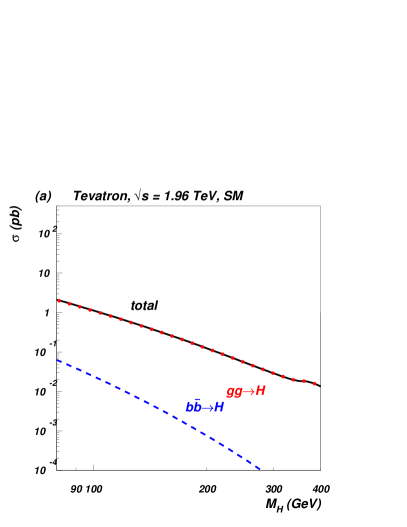
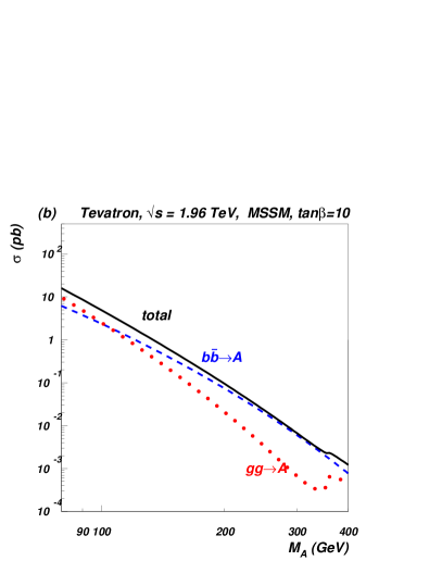
Figure 5: NLO cross sections at the Tevatron for: (a) $b\bar{b}\rightarrow H$ and $gg{\ \rightarrow^{\rhd}}\ H$ processes as well as their sum in SM; and (b) $b\bar{b}\rightarrow A$ and $gg{\ \rightarrow^{\rhd}}\ A$ , Supersymmetric CP-odd Higgs boson production in MSSM with $\tan\beta=10$.

and Fig. 6, respectively. In these figures, the dashed lines represent the cross sections for the $b\bar{b}\rightarrow H(A)$ process; the dotted lines the $gg{\ \rightarrow^{\rhd}}\ H(A)$ process; and the solid lines the combined results. Both renormalization and factorization scales are set to be $M_{H(A)}$, and the PDFs used are the CTEQ6M set [48]. For the MSSM case, the results correspond to $\tan\beta=10$ and $m_{\mathrm{top}}=178$ GeV.

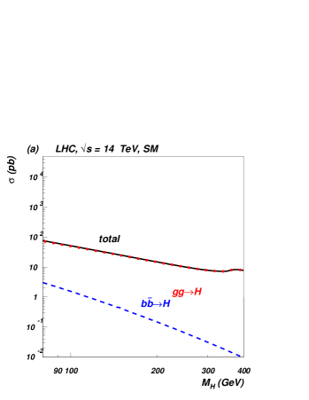
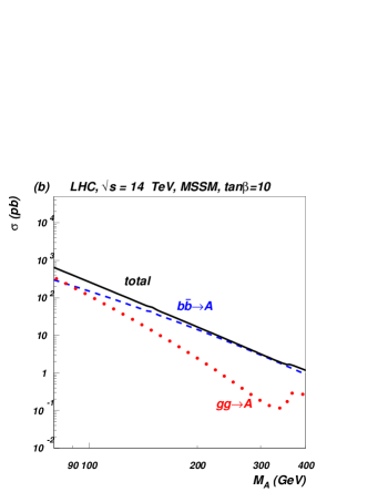
Figure 6: NLO cross sections at the LHC for: (a) $b\bar{b}\rightarrow H$ and $gg{\ \rightarrow^{\rhd}}\ H$ processes as well as their sum in SM; and (b) $b\bar{b}\rightarrow A$ and $gg{\ \rightarrow^{\rhd}}\ A$ , Supersymmetric CP-odd Higgs boson production in MSSM with $\tan\beta=10$.

One can see that in the SM case, the contribution from $b\bar{b}\rightarrow H$ is negligible compared to $gg{\ \rightarrow^{\rhd}}\ H$ . In contrast, the contribution from the Supersymmetric $b\bar{b}\rightarrow A$ process becomes important even for the moderate value of $\tan\beta\sim 10$. Except for the low Higgs mass region $M_{H}<115$ GeV, the $b\bar{b}\rightarrow A$ process is the dominant production mechanism. The ratio of $b\bar{b}\rightarrow A$ to $gg{\ \rightarrow^{\rhd}}\ A$ processes is qualitatively similar at higher values of $\tan\beta$ while the absolute value of the cross sections scales as $\tan^{2}\beta$. Relative ratios of the $b\bar{b}\rightarrow A$ and $gg{\ \rightarrow^{\rhd}}\ A$ processes at the Tevatron and LHC are very similar, while the absolute values of the production rate at the LHC is about two orders of magnitude higher then those at the Tevatron. The cross section for both processes is enhanced with high values of $\tan\beta$ and can be really large. Therefore, these processes could be useful for precision measurement of Yukawa couplings as well as bottom-quark distributions. This underlines the importance of understanding the PDF uncertainties of the cross sections for these processes.

3 Uncertainties of the Cross Sections for Higgs Production

The PDF uncertainties for Higgs production are most reliably assessed by the Lagrange multiplier (LM) method [49, 50]. It incorporates the calculated values of the Higgs cross section $\sigma$ in the global analysis, using the classic Lagrange multiplier technique. This determines the full allowed range of variation of $\sigma$ over the PDF parameter space. Our main results are obtained by this method. An alternative approach that can be applied without performing dedicated global analysis is the Hessian method [49, 51], which has been applied to the Higgs production $gg{\ \rightarrow^{\rhd}}\ H$ process in [52] and to $gg\rightarrow H\bar{b}b$ in [53]. The Hessian method is less robust because it relies on a linear approximation in the error analysis. As a part of our study, we will compare results obtained by the two methods. A brief summary of both methods is given in the Appendix.

3.1 PDF Uncertainties for the $b\bar{b}\rightarrow A$ process: the Lagrange Multiplier Method

For a given Higgs mass, the result from a LM study of the range of variation of the Higgs cross section is presented in Fig. 7. The plot shows the goodness-of-fit of the global analysis (as measured by an overall effective $\chi^{2}$ value) in constrained fits, as a function of the Higgs cross section (for the $b\bar{b}\rightarrow A$ process) over a certain range around the best-fit value. The curves represent smooth interpolations of these constrained fits (cf. the Appendix, around Eqs. (11-14), for explanation of the method). Fig. 7(left) presents results for Tevatron for $M_{A}$=100 GeV, and Fig. 7(right) presents results for LHC for $M_{A}$=400 GeV. These curves are quite close to being parabolic. This suggests that the alternative Hessian method may be a reasonable approximation.

Figure 7: Estimating the uncertainty of the Higgs cross section by the Lagrange Multiplier method: $\chi^{2}$ of the global analysis versus $\sigma(b\bar{b}\rightarrow A)$. The left plot presents results for Tevatron; the right plot for LHC.

The uncertainty range of the Higgs cross section $\sigma$ is obtained by adopting a reasonable tolerance for the global $\chi^{2}$, $T^{2}=\Delta\chi^{2}$.  Various global analysis groups (CTEQ, MRST, ZEUS, H1) have adopted values of $T^{2}$ in the range $50$-$100$, for $\sim 2000$ data points. We shall choose the more conservative value $T^{2}=100$, which we interpret as a 90% CL uncertainty range [48]. We obtain $\sigma_{+}$ and $\sigma_{-}$ as the two solutions of the equation $\chi^{2}[\sigma]=T$; and define the PDF uncertainty of the total cross section as

$$\Delta\sigma=(\sigma_{+}-\sigma_{-})/2,$$ (5)

and the relative uncertainty as

$$\delta\sigma=\Delta\sigma/\sigma\,.$$ (6)

We evaluated this relative uncertainty of the Higgs cross section, due to the input PDFs, for various values of the Higgs mass.

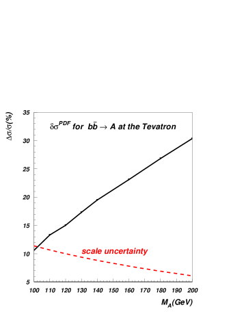
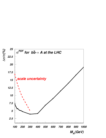
Figure 8: Results on the relative PDF uncertainty (in percentages) ${\delta\sigma}_{b\bar{b}\rightarrow A}^{PDF}$ for the Tevatron (left) and the LHC (right) as a function of Higgs boson mass. For comparison, the corresponding QCD scale uncertainty $\delta^{NNLO}$ (from Ref. [41]) are represented by dashed lines.

The results are presented in Fig. 8(left) for the Tevatron, and Fig. 8(right) for the LHC, as solid lines. For comparison, QCD scale uncertainties available for the Higgs mass range below 300 GeV from Ref. [41] are represented by dashed lines.

As one can see, there is a qualitative difference in the behavior of ${\delta\sigma^{PDF}}$ as a function of Higgs mass between the Tevatron and LHC results: at the Tevatron, ${\delta\sigma^{PDF}}$ always increases with increasing Higgs mass; while at the LHC, it has a minimum for Higgs mass around 300 GeV. To understand the reason for this behavior one can look at the uncertainty of the $gg$ luminosity function, which is directly related to the $b$-quark PDF uncertainty, since gluon splitting creates the $b$-quark parton density. This is shown in Fig. 9, for the Tevatron on the left and LHC on the right as a function the gluon-gluon invariant mass.

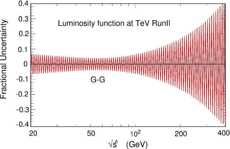
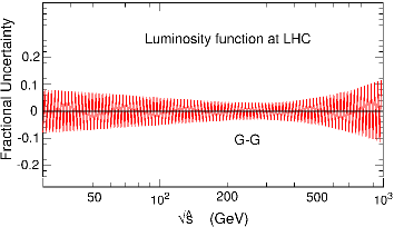
Figure 9: Fractional uncertainty of the gluon-gluon luminosity functions at the Tevatron and LHC as a function of gluon-gluon invariant mass $\sqrt{\hat{s}}$.

One can see that for $M_{A}>100$ GeV, the uncertainty of $gg$ luminosity always goes up with

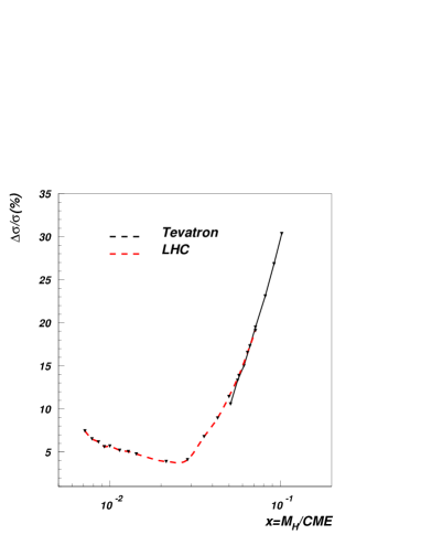
Figure 10: Relative PDF uncertainties ${\delta\sigma^{PDF}}$ of the NLO $b\bar{b}\rightarrow A$ production cross sections, as a function of $x$ for Tevatron and LHC.

the increasing Higgs boson mass, which is related to the fact that at the Tevatron the required $x$-value of PDF is already as big as 0.05 ($x=M_{A}/\sqrt{S}\gtrsim 100/1960$). Therefore with the increasing Higgs boson mass, $x$ goes up and so does ${\delta\sigma^{PDF}}$. At the LHC, however, for low $M_{A}\simeq 100$ GeV, $x_{min}\simeq 0.007$ and therefore $\delta\sigma^{PDF}$ is still big since $x$ is fairly small. When the Higgs mass increases and reaches $M_{A}\simeq 300$ GeV, ${\delta\sigma^{PDF}}$ takes the minimum at $x_{min}\simeq 0.02$. With further Higgs mass increase, ${\delta\sigma^{PDF}}$ grows similarly to its behavior at the Tevatron.

Actually, the $x$-value is the principal variable that controls the PDF uncertainty. This can be clearly seen from Fig. 10 which presents ${\delta\sigma^{PDF}}$ as a function of $x$ for Tevatron and LHC: in the $x$-region where Tevatron and LHC overlap, their PDF uncertainties are in good agreement.

3.2 Comparison of PDF to Scale Uncertainties

Included in Fig. 8 is a direct comparison of PDF uncertainties ${\delta\sigma^{PDF}}$ of the Higgs cross section with the scale uncertainty ${\delta\sigma^{SC}}$. The latter has been obtained from the QCD scale dependence of the next-to-next-leading order (NNLO) calculation of the inclusive $b\bar{b}\rightarrow A$ $+X$ processes [41]. It was found that the scale uncertainty goes down from $15\%$ to $5\%$ at the LHC and from $10\%$ to $3\%$ at the Tevatron when the Higgs mass increases from $120$ to $300$ GeV. We notice the opposite trend of those uncertainties versus Higgs boson mass at the Tevatron: ${\delta\sigma^{PDF}}$ goes up from 11% to about 30% for $M_{A}$ increasing from 100 to 200 GeV, while ${\delta\sigma^{SC}}$ decreases from $11\%$ to $6\%$. Therefore, at high $M_{A}$ values, ${\delta\sigma^{PDF}}$ becomes almost an order of magnitude larger than ${\delta\sigma^{SC}}$!

At the LHC, both ${\delta\sigma^{PDF}}$ and ${\delta\sigma^{SC}}$ decrease with the increasing $M_{A}$ in this mass range ($100-200$ GeV); but ${\delta\sigma^{SC}}$ is larger than ${\delta\sigma^{PDF}}$ by a factor $1.5-3$, depending on the Higgs mass. This plot suggests that at higher values of $M_{A}$, say $>300$ GeV, the PDF uncertainties will become dominant, similar to the situation at the Tevatron. However, NNLO scale uncertainties were not published for this Higgs mass range.

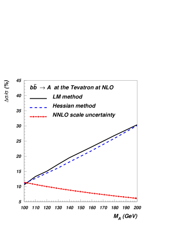
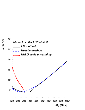
Figure 11: Relative PDF uncertainty of the $b\bar{b}\rightarrow A$ process obtained by the Hessian method (dash line), compared to that by the LM method (solid line), for Tevatron(left) and LHC (right). Scale uncertainties from Ref. [41] are presented by the dot-dash lines.

3.3 Comparison of the Lagrange Multiplier and Hessian Methods for Estimating Uncertainties

We calculated the PDF uncertainties of the cross section using the LM method, which is the most reliable one available. But it requires the full machinery of global analysis. The alternative Hessian method, utilizing a general set of eigenvector PDF sets that embody the PDF uncertainties [48], is more approximate, but more convenient [49, 51]. Fig. 11 presents the results on PDF uncertainties of the $b\bar{b}\rightarrow A$ cross section obtained by the Hessian method, compared to that obtained by the LM method for Tevatron (left) and LHC (right). As one can see, the two results are in good agreement. In Fig. 12 we present results analogous to Fig. 11 but for the $gg{\ \rightarrow^{\rhd}}\ A$ process. Again, one can see that there is good agreement between the two methods.

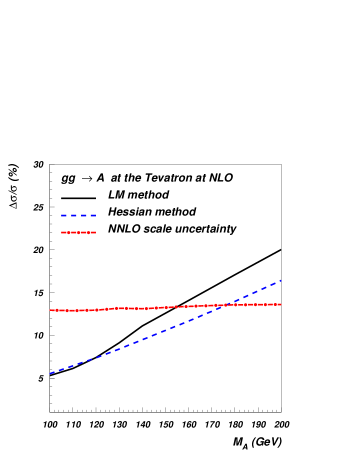
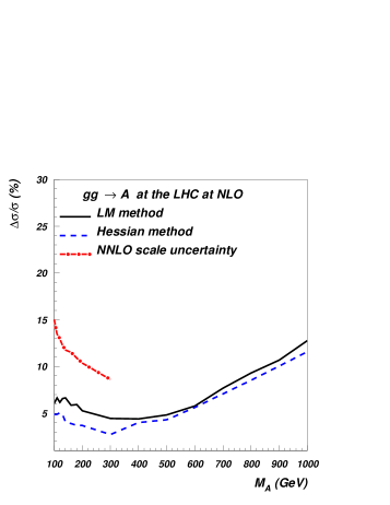
Figure 12: Relative PDF uncertainty of the $gg{\ \rightarrow^{\rhd}}\ A$ process obtained by the Hessian method (dash line), compared to that by the LM method (solid line), for Tevatron(left) and LHC (right). Scale uncertainties from Ref. [41] are presented by the dot-dash lines

3.4 Comparison of PDF Uncertainties of the $b\bar{b}\rightarrow A$ and $gg{\ \rightarrow^{\rhd}}\ A$ Processes

Notice that PDF uncertainties for the $gg{\ \rightarrow^{\rhd}}\ A$ process in comparison with $b\bar{b}\rightarrow A$ are about a factor of two smaller. To understand this fact we refer the reader to [54] where $\delta g/g$ and $\delta b/b$ uncertainties and their correlation were studied in detail. For the Tevatron, PDF uncertainties vary from $5$ to $15-20\%$ for $M_{A}$ ranging between $100$ and $200$ GeV, and dominate the scale uncertainty only for heavy Higgs of mass about $150-160$ GeV. For the LHC, PDF uncertainties are $5-6\%$ at $M_{A}=100$ GeV, decreasing to the minimum of $3-4\%$ at $M_{A}=300$ GeV and increasing again up to about 11% at $M_{A}=1000$ GeV. Available scale uncertainties for $M_{A}<300$ GeV are about a factor of two bigger than PDF uncertainties. Our results on $gg{\ \rightarrow^{\rhd}}\ A$ PDF uncertainties are in agreement with results presented in Refs. [52, 53].

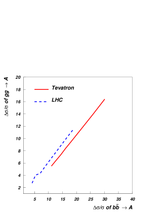
Figure 13: Correlation of PDF uncertainties for $b\bar{b}\rightarrow A$ and $gg\rightarrow A$ processes for Tevatron and LHC.

We note that the PDF uncertainties for $b\bar{b}\rightarrow A$ and for $gg{\ \rightarrow^{\rhd}}\ A$ are strongly correlated, as shown in Fig. 13, both for the Tevatron and for the LHC. This is hardly surprising, given the fact that the $b$-quarks are radiatively generated from the gluon in the way all current parton distribution functions are calculated.

Finally, Fig. 14 illustrates the NLO cross section bands for PDF uncertainties, shown in green, overlaid with the NNLO scale uncertainties, shown in red. One can see that for low Higgs mass, the scale uncertainties are comparable or dominant for both colliders and both processes, while for heavier Higgses, PDF uncertainties are significantly larger than the scale uncertainties.

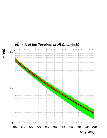
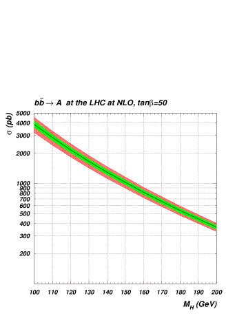
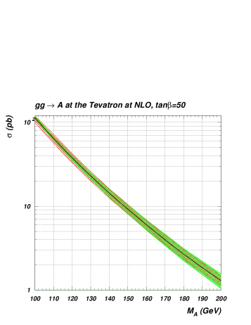
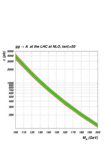
Figure 14: NLO cross section bands for PDF uncertainties, shown in green, overlaid on NNLO scale uncertainties, shown in red. The upper two frames show results for $b\bar{b}\rightarrow A$ at Tevatron (left) and LHC (right), while lower two frames show results for $gg\rightarrow A$ process at Tevatron (left) and LHC (right). respectively.

4 Conclusions

The role of $b\bar{b}\rightarrow A$ and $gg{\ \rightarrow^{\rhd}}\ A$ processes may be central for the Higgs boson search. Therefore the correct understanding of uncertainties of their production rate is crucial.

We found that the PDF uncertainty of $b\bar{b}\rightarrow A$ is about a factor two larger than the PDF uncertainty for $gg{\ \rightarrow^{\rhd}}\ A$ . It was found that at the Tevatron, PDF uncertainty dominates the scale uncertainty for $M_{A}>$130 GeV and could be as large as $30\%$ for $M_{A}$=200 GeV, which is an order of magnitude larger than the NNLO scale uncertainty. At the LHC the scale uncertainty is dominant and could be as big as 15% for $M_{A}<$300 GeV. In this region one could expect large Higgs production rates that would statistically allow the precision measurement of Higgs Yukawa couplings. Therefore, higher order corrections would be necessary in this case for better theoretical control of the cross section. For $M_{H}>$300 GeV, PDF uncertainty is likely to dominate at the LHC, similarly to the picture for the Tevatron. These results underline the importance of gaining better control of the PDF uncertainties, in the study of Higgs physics in the next generation of Colliders.

We have also found that the Lagrange Multiplier and Hessian methods for assessing PDF uncertainties are in good agreement with each other.

APPENDIX

In this appendix we briefly review the methods of global PDF fit and estimation of PDF uncertainties using Hessian and Lagrange multiplier methods.

Parton distributions which are being used for the SM and new physics predictions are obtained from global analysis using a “best-fit” paradigm for which the PDF is selected for the minimum of the chosen $\chi^{2}$ function. The main question is what are the uncertainties of those PDFs?

In our study we are using two methods for this purpose, namely Hessian method [49, 51] and method of Lagrange multiplier [50] which as it was discussed in Ref. [48], overcomes various problems of standard error analysis. In particular, in Ref. [48], the authors presented a reliable way of understanding the behavior of $\chi^{2}$ function in the neighborhood of the global minimum, providing the way of correct understanding of the PDF uncertainties in the prediction of the cross sections.

We summarize here briefly both methods. Both methods use a chi-square function $\chi^{{2}}$ is defined by

$$\chi^{2} = \sum_{e}\chi_{e}^{2}(a,r),\mbox{\ \ \ where \ \ \ }\chi_{e}^{2}(a,r)=\sum_{i}\frac{\left[D_{i}-\sum_{k}r_{k}\beta_{ki}-T_{i}(a)\right]^{2}}{\alpha_{i}^{2}}+\sum_{k}r_{k}^{2},$$ (7)

where $e$ labels an experimental data set and $i$ labels a data point in each particular data set. $D_{i}$ is the data value, $\alpha_{i}$ is the uncorrelated error, and $\beta_{ki}$ is the $k$th correlated systematic error; these numbers are published by the experimental collaboration. $T_{i}(a)$ is the theoretical value, a function of a set of $n$ PDF parameters, $\{a_{1},\dots,a_{n}\}$. Also, $\{r_{k}\}$ is a set of Gaussian random variables and $r_{k}\beta_{ki}$ is a (correlated) shift applied to $D_{i}$ to represent the $k$th systematic error. We minimize the function $\chi^{{2}}(a,r)$ with respect to both the PDF parameters $\{a\}$ and the systematic shift variables $\{r_{k}\}$. The result yields both the standard PDF model with parameters $\{a_{0}\}$, and the optimal shifts $\{\widehat{r}_{k}\}$ to bring theory and data into agreement. This minimum of $\chi^{{2}}$ represents the best fit to the data [48].

Hessian method for analysis of PDF uncertainty in the neighborhood of the minima of $\chi^{2}$ involves the Hessian matrix

$$H_{ij}=\frac{1}{2}\frac{\partial^{2}{\chi}^{2}_{0}}{\partial{a}_{i}\partial{a}_{j}}$$ (8)

calculated at the minimum of $\chi^{2}_{0}$. The next step is to diagonalize $H_{ij}$ and to find its eigenvectors. Then for each eigenvector we have two displacements from $\{a_{0}\}$ (in the $+$ and $-$ directions along the vector) denoted $\{a^{+}_{i}\}$ and $\{a^{-}_{i}\}$ for the $i$th eigenvector. At these points, ${\chi}^{2}_{\pm}={\chi}_{0}^{2}+T^{2}$ and $T$ parametrizes the tolerance. The appropriate choice of tolerance $T$ cannot be decided without a further, more detailed, analysis of the quality of the global fits. After studying a number of examples [51, 50], we concluded that a rather large tolerance, $T\sim 10$, represents a realistic estimate of the PDF uncertainty.

One can show that in a linear approximation, the uncertainty $\delta X$ for any quantity $X$, which depends on PDF, can be expressed as

$$\left(\delta{X}\right)^{2}=T^{2}\sum_{i,j}\left(H^{-1}\right)_{ij}\frac{\partial{X}}{\partial{a}_{i}}\frac{\partial{X}}{\partial{a}_{j}};$$ (9)

or, in terms of the eigenvector basis sets,

$$\left(\delta{X}\right)^{2}=\frac{1}{4}\sum_{k=1}^{n}\left[X(a^{+}_{i})-X(a^{-}_{i})\right]^{2}.$$ (10)

representing the master equation defined in [50]. One should point out again, that equation (10) is based on a linear approximation: ${\chi}^{2}(a)$ is assumed to be a quadratic function of the parameters $\{a\}$, and $X(a)$ is assumed to be linear. This approximation is not strictly valid in general.

The essence of the Lagrange multiplier method is the introduction of the Lagrange multiplier variable $\lambda$ and minimizing the function

$$\chi^{2}_{\lambda}(\lambda,a)=\chi^{2}(a)+\lambda X(a)$$ (11)

with respect to the original $n$ parameters $\{a\}$ for fixed values of $\lambda$. In Eq.11 X(a) is some observable as in the example for Hessian method. Minimization of $\chi^{2}_{\lambda}(\lambda,a)$ for various values of $\lambda$ allows to find the parametric relationship between $\chi^{2}(a)$ and $X(a)$, .i.e.

$$\chi^{2}_{\lambda}(\lambda,a_{0})=\chi^{2}(a_{0})+\lambda X(a_{0})\Longrightarrow X=X(\chi^{2}(a_{0},\lambda)),$$ (12)

where $a_{0}$ is the set of parameter values $\{a\}$ for each particular value of $\lambda$. Eq. (12) is the key point of LM method since for given value of tolerance

$$\Delta\chi^{2}=\chi^{2}(a_{0},\lambda^{\Delta}_{\pm})-\chi^{2}(a_{0},0)$$ (13)

which would correspond to some two values $\lambda^{\Delta}_{\pm}$, one can find the respective variation of the observable $X$:

$$\delta X_{+}=X(\chi^{2}(a_{0},\lambda^{\Delta}_{+}))-X(\chi^{2}(a_{0},0)),\ \ \delta X_{-}=X(\chi^{2}(a_{0},\lambda^{\Delta}_{-}))-X(\chi^{2}(a_{0},0))\,.$$ (14)

The LM method for calculating $\delta X_{\pm}$ is more robust in general since it does not approximate $X(a)$ and $\chi^{2}(a)$ by linear and quadratic dependence on $\{a\}$, respectively, around the minimum.

References

- [1] R. M. Barnett, G. Senjanovic, and D. Wyler, Tracking down higgs scalars with enhanced couplings, Phys. Rev. D30 (1984) 1529.
- [2] P. N. Pandita, Are higgs couplings enhanced in minimal supergravity models?, Phys. Lett. B151 (1985) 51.
- [3] P. Q. Hung and S. Pokorski, Enhanced higgs boson production at the tevatron, . FERMILAB-PUB-87-211-T.
- [4] L. H. W. Group, “Searches for the neutral higgs bosons of the mssm: Preliminary combined results using lep data collected at energies up to 209-gev.” hep-ex/0107030, 2001.
- [5] R. N. Mohapatra, “Unification and supersymmetry.” hep-ph/9911272, 1999.
- [6] M. Gell-Mann, P. Ramond, and R. Slansky, Color embeddings, charge assignments, and proton stability in unified gauge theories, Rev. Mod. Phys. 50 (1978) 721.
- [7] H. Fritzsch and P. Minkowski, Unified interactions of leptons and hadrons, Ann. Phys. 93 (1975) 193–266.
- [8] S. Raby, Desperately seeking supersymmetry (susy), Rept. Prog. Phys. 67 (2004) 755–811, [hep-ph/0401155].
- [9] G. Altarelli and F. Feruglio, Models of neutrino masses and mixings, New J. Phys. 6 (2004) 106, [hep-ph/0405048].
- [10] B. Ananthanarayan, G. Lazarides, and Q. Shafi, Top mass prediction from supersymmetric guts, Phys. Rev. D44 (1991) 1613–1615.
- [11] G. Anderson, S. Raby, S. Dimopoulos, L. J. Hall, and G. D. Starkman, A systematic so(10) operator analysis for fermion masses, Phys. Rev. D49 (1994) 3660–3690, [hep-ph/9308333].
- [12] M. Carena, M. Olechowski, S. Pokorski, and C. E. M. Wagner, Electroweak symmetry breaking and bottom - top yukawa unification, Nucl. Phys. B426 (1994) 269–300, [hep-ph/9402253].
- [13] R. Rattazzi and U. Sarid, The unified minimal supersymmetric model with large yukawa couplings, Phys. Rev. D53 (1996) 1553–1585, [hep-ph/9505428].
- [14] B. Ananthanarayan, Q. Shafi, and X. M. Wang, Improved predictions for top quark, lightest supersymmetric particle, and higgs scalar masses, Phys. Rev. D50 (1994) 5980–5984, [hep-ph/9311225].
- [15] T. Blazek, S. Raby, and K. Tobe, Neutrino oscillations in a predictive susy gut, Phys. Rev. D60 (1999) 113001, [hep-ph/9903340].
- [16] T. Blazek, R. Dermisek, and S. Raby, Predictions for higgs and susy spectra from so(10) yukawa unification with mu ¿ 0, Phys. Rev. Lett. 88 (2002) 111804, [hep-ph/0107097].
- [17] T. Blazek, R. Dermisek, and S. Raby, Yukawa unification in so(10), Phys. Rev. D65 (2002) 115004, [hep-ph/0201081].
- [18] H. Baer, M. A. Diaz, J. Ferrandis, and X. Tata, Sparticle mass spectra from so(10) grand unified models with yukawa coupling unification, Phys. Rev. D61 (2000) 111701, [hep-ph/9907211].
- [19] H. Baer et. al., Yukawa unified supersymmetric so(10) model: Cosmology, rare decays and collider searches, Phys. Rev. D63 (2001) 015007, [hep-ph/0005027].
- [20] H. Baer and J. Ferrandis, Supersymmetric so(10) gut models with yukawa unification and a positive mu term, Phys. Rev. Lett. 87 (2001) 211803, [hep-ph/0106352].
- [21] D. Auto et. al., Yukawa coupling unification in supersymmetric models, JHEP 06 (2003) 023, [hep-ph/0302155].
- [22] D. Auto, H. Baer, A. Belyaev, and T. Krupovnickas, “Reconciling neutralino relic density with yukawa unified supersymmetric models.” hep-ph/0407165, 2004.
- [23] S. Dawson, A. Djouadi, and M. Spira, Qcd corrections to susy higgs production: The role of squark loops, Phys. Rev. Lett. 77 (1996) 16–19, [hep-ph/9603423].
- [24] R. V. Harlander and M. Steinhauser, Hadronic higgs production and decay in supersymmetry at next-to-leading order, Phys. Lett. B574 (2003) 258–268, [hep-ph/0307346].
- [25] R. Harlander and M. Steinhauser, Effects of susy-qcd in hadronic higgs production at next- to-next-to-leading order, Phys. Rev. D68 (2003) 111701, [hep-ph/0308210].
- [26] R. V. Harlander and M. Steinhauser, Supersymmetric higgs production in gluon fusion at next-to- leading order, JHEP 09 (2004) 066, [hep-ph/0409010].
- [27] M. Carena, D. Garcia, U. Nierste, and C. E. M. Wagner, b –¿ s gamma and supersymmetry with large tan(beta), Phys. Lett. B499 (2001) 141–146, [hep-ph/0010003].
- [28] A. Belyaev, D. Garcia, J. Guasch, and J. Sola, Prospects for heavy supersymmetric charged higgs boson searches at hadron colliders, JHEP 06 (2002) 059, [hep-ph/0203031].
- [29] J. C. Collins and W.-K. Tung, Calculating heavy quark distributions, Nucl. Phys. B278 (1986) 934.
- [30] F. I. Olness and W.-K. Tung, When is a heavy quark not a parton?, . To appear in Proc. of 1988 Lake Louise Winter Inst., Quantum Chromodynamics: Theory and Experiment, Lake Louise, Canada, Mar 6-12, 1988.
- [31] R. M. Barnett, H. E. Haber, and D. E. Soper, Ultraheavy particle production from heavy partons at hadron colliders, Nucl. Phys. B306 (1988) 697.
- [32] J. Amundson, C. Schmidt, W.-K. Tung, and X. Wang, Charm production in deep inelastic scattering from threshold to high q**2, JHEP 10 (2000) 031, [hep-ph/0005221].
- [33] J. L. Diaz-Cruz, H.-J. He, T. Tait, and C. P. Yuan, Higgs bosons with large bottom yukawa coupling at tevatron and lhc, Phys. Rev. Lett. 80 (1998) 4641–4644, [hep-ph/9802294].
- [34] C. Balazs, J. L. Diaz-Cruz, H. J. He, T. Tait, and C. P. Yuan, Probing higgs bosons with large bottom yukawa coupling at hadron colliders, Phys. Rev. D59 (1999) 055016, [hep-ph/9807349].
- [35] D. Dicus, T. Stelzer, Z. Sullivan, and S. Willenbrock, Higgs boson production in association with bottom quarks at next-to-leading order, Phys. Rev. D59 (1999) 094016, [hep-ph/9811492].
- [36] J. Campbell, R. K. Ellis, F. Maltoni, and S. Willenbrock, Higgs boson production in association with a single bottom quark, Phys. Rev. D67 (2003) 095002, [hep-ph/0204093].
- [37] F. Maltoni, Z. Sullivan, and S. Willenbrock, Higgs-boson production via bottom-quark fusion, Phys. Rev. D67 (2003) 093005, [hep-ph/0301033].
- [38] E. Boos and T. Plehn, Higgs-boson production induced by bottom quarks, Phys. Rev. D69 (2004) 094005, [hep-ph/0304034].
- [39] H.-S. Hou, W.-G. Ma, P. Wu, L. Wang, and R.-Y. Zhang, Higgs-boson production associated with a single bottom quark in supersymmetric qcd, Phys. Rev. D68 (2003) 035016, [hep-ph/0307055].
- [40] S. Dittmaier, M. Kramer, and M. Spira, Higgs radiation off bottom quarks at the tevatron and the lhc, Phys. Rev. D70 (2004) 074010, [hep-ph/0309204].
- [41] R. V. Harlander and W. B. Kilgore, Higgs boson production in bottom quark fusion at next-to- next-to-leading order, Phys. Rev. D68 (2003) 013001, [hep-ph/0304035].
- [42] S. Dawson, C. B. Jackson, L. Reina, and D. Wackeroth, Exclusive higgs boson production with bottom quarks at hadron colliders, Phys. Rev. D69 (2004) 074027, [hep-ph/0311067].
- [43] M. Kramer, Associated higgs production with bottom quarks at hadron colliders, Nucl. Phys. Proc. Suppl. 135 (2004) 66–70, [hep-ph/0407080].
- [44] B. Field, Higgs boson resummation via bottom quark fusion, hep-ph/0407254.
- [45] S. Dawson, C. B. Jackson, L. Reina, and D. Wackeroth, Higgs boson production with one bottom quark jet at hadron colliders, Phys. Rev. Lett. 94 (2005) 031802, [hep-ph/0408077].
- [46] C. Balazs, H.-J. He, and C. P. Yuan, QCD corrections to scalar production via heavy quark fusion at hadron colliders, Phys. Rev. D60 (1999) 114001, [hep-ph/9812263].
- [47] M. Spira, Higlu and hdecay: Programs for higgs boson production at the lhc and higgs boson decay widths, Nucl. Instrum. Meth. A389 (1997) 357–360, [hep-ph/9610350].
- [48] J. Pumplin et. al., New generation of parton distributions with uncertainties from global qcd analysis, JHEP 07 (2002) 012, [hep-ph/0201195].
- [49] J. Pumplin, D. R. Stump, and W. K. Tung, Multivariate fitting and the error matrix in global analysis of data, Phys. Rev. D65 (2002) 014011, [hep-ph/0008191].
- [50] D. Stump et. al., Uncertainties of predictions from parton distribution functions. i: The lagrange multiplier method, Phys. Rev. D65 (2002) 014012, [hep-ph/0101051].
- [51] J. Pumplin et. al., Uncertainties of predictions from parton distribution functions. ii: The hessian method, Phys. Rev. D65 (2002) 014013, [hep-ph/0101032].
- [52] A. Djouadi and S. Ferrag, Pdf uncertainties in higgs production at hadron colliders, Phys. Lett. B586 (2004) 345–352, [hep-ph/0310209].
-
[53]
2005.
Chris Jackson, talk given at TeV4LHC workshop, February 2005,
http://www.hep.fsu.edu/~jackson/Tev4LHC_bpdf.pdf. - [54] Z. Sullivan and P. M. Nadolsky, Heavy-quark parton distribution functions and their uncertainties, eConf C010630 (2001) P511, [hep-ph/0111358].