UB-ECM-PF-05-17
August 2005

Fit to the Bjorken, Ellis-Jaffe and Gross-Llewellyn-Smith sum rules in a renormalon based approach

Abstract

We study the large order behaviour in perturbation theory of the Bjorken, Ellis-Jaffe and Gross-Llewellyn-Smith sum rules. In particular, we consider their first infrared renormalons, for which we obtain their analytic structure with logarithmic accuracy and also an approximate determination of their normalization constant. Estimates of higher order terms of the perturbative series are given. The Renormalon subtracted scheme is worked out for these observables and compared with experimental data. Overall, good agreement with experiment is found. This allows us to obtain ${\hat{a}}_{0}$ and some higher-twist non-perturbative constants from experiment: ${\hat{a}}_{0}=0.141\pm 0.089$; $f_{3,\rm RS}(1\;{\rm GeV})=-0.124^{+0.137}_{-0.142}$ GeV².
PACS numbers: 11.55.Hx, 12.38.Bx, 12.38.Cy, 12.38.Qk, 13.60.Hb

1 Introduction

Deep Inelastic Scattering (DIS) is one of the few places where one can test, on a very solid theoretical ground, asymptotic freedom and the operator product expansion against experiment. This is so because, for the moments of the different structure functions, the transfer momentum lies in the euclidean region and far away of the physical cuts (for $Q^{2}$ large). Therefore, the theoretical predictions do not rely on any kind of quark-hadron duality and may provide with solid and very clean determinations of $\alpha_{\rm s}$ and some non-perturbative matrix elements. Equally interesting is the study of the interplay between the perturbative and non-perturbative regime. This can only be done if a full control on the perturbative series is achieved.

Within DIS, special consideration deserve the sum rules for which the matrix elements are related to symmetry generators (in this case they can be computed in absolute value within perturbation theory), like the Gross-Llewellyn-Smith (GLS) sum rule [2], or to some low energy constants (which can be directly measured from experiment), like the Bjorken sum rule [3]. In this paper, we will concentrate on the Bjorken, Ellis-Jaffe [4] and GLS sum rules. Their leading-twist term has been computed with next-to-next-to-leading order (NNLO) accuracy and they have been measured with increasingly good accuracy over the years.

By the Operator Product Expansion, the short- and long-distance contributions are separated and a sum rule, M, can be expressed in the following way:

$$M=C{<}J{>}+B\frac{{<}R{>}}{Q^{2}}+\ldots\,,$$ (1)

with short-distance Wilson coefficients $C,B,$ $\ldots$ and long-distance matrix elements ${<}J{>},$ ${<}R{>},$ $\ldots$. The perturbative series of $C$ are expected to be asymptotic and, therefore, to diverge for a high enough order in perturbation theory. Moreover, in schemes without strict separation of large and small momenta, such as $\overline{\mathrm{MS}}$, they are believed to be non-Borel summable. This is because when calculating the matching coefficients $C$, …, the integrals run over all loop momenta, including small ones. Therefore, they also contain, in addition to the main short-distance contributions, contributions from large distances, where perturbation theory is ill-defined. These contributions produce infrared renormalon singularities [5], factorially growing contributions to coefficients of the perturbative series, which lead to ambiguities $\sim\left(\Lambda_{\mathrm{QCD}}/Q\right)^{2n}$ in the matching coefficients $C$, …. Similarly, matrix elements of higher-dimensional operators ${<}R{>}$, …also contain, in addition to the main large-distance contributions, contributions from short distances, which produce ultraviolet-renormalon singularities. They lead to ambiguities of the order $\Lambda_{\mathrm{QCD}}^{2n}$ times lower-dimensional matrix elements (e.g., ${<}J{>}$). These two kinds of renormalon ambiguities should cancel in physical observables [6, 7, 8, 9, 10, 11], in this case M.

The intrinsic (minimal) error associated to the perturbative series is of the order of the higher twist correction. Thus, one can not unambiguously determine the higher twist terms, unless a prescription to deal with the perturbative series that has power-like accuracy is given. In this paper we will adapt to this case the prescription used for heavy quark physics in Refs. [12, 13, 14]. The idea is that the leading divergent behaviour of the perturbative series is related to the closest singularities in the Borel plane of its Borel transform. In heavy quark physics, they lie on the positive axis (infrared renormalons). In the case of the sum rules considered in this paper, the closest singularities lie on the positive and negative axis at equal distance to the origin. We will assume that the one in the positive axis will dominate the asymptotics of the perturbative series. Since these singularities cancel against the ultraviolet renormalons of the low energy dynamics of the twist-4 operators, the proposal will be to shift the singularities from the perturbative series to the twist-4 operators. We will refer to this prescription as the Renormalon Subtracted (RS) scheme and apply it to the Bjorken, Ellis-Jaffe and GLS sum rules. We will obtain the contribution of the leading infrared renormalon, subtract it from the perturbative series and add it to the low energy matrix elements, in our case, to the twist-4 operators. In this way one enlarges the range of convergence of the Borel transform of the perturbative series, which can be defined with power-like accuracy. This procedure has proven to be extremely successful in heavy quark physics, where it has been shown that perturbation theory works very well and good determinations of non-perturbative subleading corrections have been obtained using either lattice or experimental data. One should be aware, however, that in heavy quark physics one was in an optimal situation, since the singularity in the Borel plane was quite close to the origin ($u=1/2$). We are now going to be in a less optimal situation, since the closest singularities lie at $u=\pm 1$. The physical situation is also completely different since now we are talking of a system made with light fermions. Therefore, it is interesting to investigate if a similar improvement is obtained in this case. We will do so in this paper.

The paper is organized as follows. In the next section we will introduce the relevant sum rules. In Sect. 3 the Borel transform of the first infrared renormalon of the leading-twist Wilson coefficient will be calculated with leading log accuracy, as well as the normalization constant and estimates of the higher order terms of the perturbative series. The RS scheme will be worked out in Sect. 4. In Sect. 5 the comparison with the experimental data will be done allowing us the extraction of some non-perturbative matrix elements. Finally, the conclusions are presented in Sect. 6.

2 Sum Rules

The Bjorken and Ellis-Jaffe sum rules are related to polarized deep inelastic electron-nucleon scattering, which is described by the hadronic tensor

$$W_{\mu\nu} = \frac{1}{4\pi}\int d^{4}ze^{iqz}\langle p,s|J_{\mu}(z)J_{\nu}(0)|p,s\rangle$$ (2)

$$= \left(-g_{\mu\nu}+\frac{q_{\mu}q_{\nu}}{q^{2}}\right)F_{1}(x,Q^{2})+\left(p_{\mu}-\frac{p\cdot q}{q^{2}}q_{\mu}\right)\left(p_{\nu}-\frac{p\cdot q}{q^{2}}q_{\nu}\right)\frac{1}{p\cdot q}F_{2}(x,Q^{2})$$

$$+i\epsilon_{\mu\nu\rho\sigma}q_{\rho}\left(\frac{s_{\sigma}}{p\cdot q}g_{1}(x,Q^{2})+\frac{s_{\sigma}p\cdot q-p_{\sigma}q\cdot s}{(p\cdot q)^{2}}g_{2}(x,Q^{2})\right)\,.$$

Here $J_{\mu}=\sum_{i=1}^{n_{f}}e_{i}\overline{\psi_{i}}\gamma_{\mu}\psi_{i}$ is the electromagnetic quark current where $e_{i}=2/3,-1/3,-1/3,\cdots$ is the electromagnetic charge of a quark with the corresponding flavour, $u$, $d$, $s$. $x=Q^{2}/(2p\cdot q)$ is the Bjorken scaling variable and $Q^{2}=-q^{2}$ is the square of the transferred momentum. $|p,s\rangle$ is the nucleon state that is normalized as $\langle p,s|p^{\prime},s^{\prime}\rangle$ $=2p^{0}(2\pi)^{3}\delta^{(3)}(p-p^{\prime})\delta_{ss^{\prime}}$. The polarization vector of the nucleon is expressed as $s_{\sigma}=\overline{U}(p,s)\gamma_{\sigma}\gamma_{5}U(p,s)$ where $U(p,s)$ is the nucleon spinor $\overline{U}(p,s)U(p,s)=2m_{N}$.

The Ellis-Jaffe sum rule then reads

$$M_{1}^{p/n}(Q^{2})=\left(\pm\frac{1}{12}g_{A}+\frac{1}{36}a_{8}\right)C_{B}(\alpha_{\rm s})+\frac{1}{9}{\hat{a}_{0}}C_{EJS}(\alpha_{\rm s})$$ (3)

$$-\frac{8}{9Q^{2}}\left[\left(\pm\frac{1}{12}f_{3}(Q_{0})+\frac{1}{36}f_{8}(Q_{0})\right)\left(\frac{\alpha_{s}(Q_{0}^{2})}{\alpha_{s}(Q^{2})}\right)^{-\frac{\gamma_{NS}^{0}}{2\beta_{0}}}\left(1+{\cal O}(\alpha_{\rm s})\right)+\right.$$

$$\left.+\frac{1}{9}f_{0}(Q_{0})\left(\frac{\alpha_{s}(Q_{0}^{2})}{\alpha_{s}(Q^{2})}\right)^{-\frac{1}{2\beta_{0}}(\gamma_{NS}^{0}+\frac{4}{3}N_{f})}\left(1+{\cal O}(\alpha_{\rm s})\right)\right]+{\cal O}\left({1\over Q^{4}}\right),$$

and the Bjorken sum rule is the difference between the proton and neutron sum rule:

$$M_{1}^{B}\equiv M_{1}^{p}(Q^{2})-M_{1}^{n}(Q^{2})={g_{A}\over 6}C_{B}(\alpha_{\rm s})-{4\over 27}{1\over Q^{2}}f_{3}(Q_{0})\left[{\alpha_{\rm s}(Q_{0}^{2})\over\alpha_{\rm s}(Q^{2})}\right]^{-\gamma_{\rm NS}^{0}\over 2\beta_{0}}\left(1+{\cal O}(\alpha_{\rm s})\right)+{\cal O}\left({1\over Q^{4}}\right)\,,$$ (4)

where the definitions are the following:

$$\gamma_{NS}^{0}={16\over 3}C_{F};\qquad\gamma_{S}^{0}=\gamma_{NS}^{0}+{4\over 3}n_{f};$$ (5)

$$C_{X}(Q)=1+\sum_{s=0}^{\infty}C_{X}^{(s)}\alpha_{\rm s}^{s+1}(\nu)\,,$$ (6)

and $X=\{B$, $EJ$, $GLS\}$, the latter to be defined below. For the Bjorken sum rule, the $\alpha_{s}$ correction [15], the $\alpha_{s}^{2}$ correction [16], and the $\alpha_{s}^{3}$ correction [17] have been calculated in the leading twist approximation. Higher twist corrections have also been calculated [18]. The Ellis-Jaffe sum rule for the proton and neutron was calculated to order $\alpha_{s}$ [19], to order $\alpha_{s}^{2}$ [20] and to order $\alpha_{s}^{3}$ [21] in the leading twist approximation. Power corrections were calculated in [22]. The LO renormalization group running of the twist-4 operators have been computed in Ref. [23]. The non-perturbative matrix elements are defined in the following way:

$$\begin{array}[]{llrll}|g_{A}|s_{\sigma}&=&2\langle p,s|J^{5,3}_{\sigma}|p,s\rangle&=&(\Delta u-\Delta d)s_{\sigma},\\ a_{8}s_{\sigma}&=&2\sqrt{3}\langle p,s|J^{5,8}_{\sigma}|p,s\rangle&=&(\Delta u+\Delta d-2\Delta s)s_{\sigma},\\ a_{0}(\mu^{2})s_{\sigma}&=&\langle p,s|J^{5}_{\sigma}|p,s\rangle&=&(\Delta u+\Delta d+\Delta s)s_{\sigma}.\end{array}$$

where $J_{\sigma}^{5,a}(x)=\overline{\psi}\gamma_{\sigma}\gamma_{5}t^{a}\psi(x)$ is the non-singlet axial current, where $t^{a}$ is a generator of the flavour group, and $J_{\sigma}^{5}(x)=\sum_{i=1}^{n_{f}}\overline{\psi_{i}}\gamma_{\sigma}\gamma_{5}\psi_{i}(x)$ is the singlet axial current. $|g_{A}|$ is the absolute value of the constant of the neutron beta-decay, $|g_{A}/g_{V}|=F+D=1.2695\pm 0.0029$ [24]. $a_{8}=3F-D=0.572\pm 0.019$ is the hyperon decay constant. The matrix element of the singlet axial current $a_{0}(\mu^{2})$ will be redefined in a proper invariant way as a constant ${\hat{a}}_{0}$:

$${\hat{a}}_{0}={\rm exp}\left(-2\int^{\alpha_{\rm s}(\nu)}d\alpha_{\rm s}^{\prime}{\gamma^{s}(\alpha_{\rm s}^{\prime})\over\beta(\alpha_{\rm s}^{\prime})}\right)a_{0}(\nu)\,.$$ (7)

We use the notation $\Delta q(\mu^{2})s_{\sigma}=\langle p,s|\overline{q}\gamma_{\sigma}\gamma_{5}q|p,s\rangle$, $q=u,d,s$, for the polarized quark distributions. $f_{0}$, $f_{3}$ and $f_{8}$ are the twist-4 counter parts of $a_{0}$, $a_{3}$ and $a_{8}$. $f_{i}$’s are scale dependent and here they are defined at $Q_{0}^{2}$, i.e. $f_{i}$ is the reduced matrix element of $R_{2\sigma}^{i}$, renormalized at $Q_{0}^{2}$, which is defined for the general flavor indices, with $t^{i}$ being the flavor matrices, as

$$R_{2\sigma}^{i}=g\overline{\psi}\tilde{G}_{\sigma\nu}\gamma^{\nu}t^{i}\psi,\quad\langle p,s|R_{2\sigma}^{i}|p,s\rangle=f_{i}s_{\sigma}\quad(i=0,\cdots,8),$$ (8)

and $\tilde{G}_{\mu\nu}=\frac{1}{2}\varepsilon_{\mu\nu\alpha\beta}G^{\alpha\beta}$ is the dual field strength.

In the left-hand side of equations (3-4) target-mass effects have been included using the Nachtmann variable [26]. They read

$$M_{1}^{N}(Q^{2}) \equiv \int_{0}^{1}dx{\xi^{2}\over x^{2}}\left\{g_{1}^{N}(x,Q^{2})\left[{x\over\xi}-{1\over 9}{m_{N}^{2}x^{2}\over Q^{2}}{\xi\over x}\right]\right.-\left.g_{2}^{N}(x,Q^{2})~{}{m_{N}^{2}x^{2}\over Q^{2}}{4\over 3}\right\}~{}~{}~{}~{}$$ (9)

$$=\int_{0}^{1}g_{1}^{N}(x,Q^{2})dx+{\mu_{4}^{N}\over Q^{2}}+{\cal O}\left({1\over Q^{4}}\right)=\Gamma_{1}^{N}(Q^{2})+{\mu_{4}^{N}\over Q^{2}}+{\cal O}\left({1\over Q^{4}}\right)$$

where $\xi=2x/\left(1+\sqrt{1+4m_{N}^{2}x^{2}/Q^{2}}\right)$ is the Nachtmann scaling variable, $m_{N}$ is the nucleon mass. The quantity $M_{1}$ is the first Nachtmann moment of $g_{1}$ that absorbs all the target mass corrections, $\sim(m_{N}^{2}/Q^{2})^{n}$, and

$$\mu_{4}^{N} = -\frac{m_{N}^{2}}{9}\left(a^{N}_{2}+4d^{N}_{2}\right),$$ (10)

where $a_{2}^{N}$ is the target mass correction given by the $x^{2}$-weighted moment of the leading-twist $g_{1}$ structure function, and $d_{2}^{N}$ is a twist-3 matrix element given by

$$d^{N}_{2} = \int_{0}^{1}dx~{}x^{2}\left(2g^{N}_{1}+3g^{N}_{2}\right).$$ (11)

We will consider the Ellis-Jaffe proton sum rule and the Bjorken sum rule. For the former we will use the data points given in Ref. [27], which are already given in terms of $M_{1}^{p}$, and for the latter we will use the data points given in Ref. [28], which used the values:

$$d_{2}^{p-n}=-0.0029\,,\qquad a_{2}^{p-n}=0.0279\,.$$ (12)

If one also considers DIS of neutrinos with nucleons, the GLS sum rule appears, for which the leading twist have been computed with NNLO accuracy (see for instance [29]):

$$M_{3}^{GLS}\equiv{1\over 2}\left(M_{3}^{p}(Q^{2})+M_{3}^{n}(Q^{2})\right)=3C_{GLS}(\alpha_{\rm s})-\frac{8}{9}\left(\frac{\alpha_{s}(Q_{0}^{2})}{\alpha_{s}(Q^{2})}\right)^{-\frac{\gamma_{NS}^{0}}{2\beta_{0}}}\frac{\langle\langle O^{{\rm S}(p+n)}_{5}\rangle\rangle(Q_{0})}{Q^{2}}\,,$$ (13)

where

$$M_{3}^{N}(Q^{2}) = \frac{1}{3}\int_{0}^{1}dx\;F_{3}^{\nu N}(x;Q^{2})\frac{\zeta^{2}}{x^{2}}\left[1+2\left(1+\frac{4m_{N}^{2}x^{2}}{Q^{2}}\right)^{1/2}\right]$$ (14)

$$= \int_{0}^{1}dx\;F_{3}^{\nu N}(x;Q^{2})\left[1-\frac{2}{3}\frac{m_{N}^{2}x^{2}}{Q^{2}}+{\cal O}\left(\frac{m_{N}^{4}}{Q^{4}}\right)\right]\ ,$$

$$\langle P|O^{{\rm S}}_{5\mu}|P\rangle_{{\rm\scriptstyle spin}\atop{\rm\scriptstyle averaged}}\equiv 2P_{\mu}\langle\langle O^{{\rm S}}_{5}\rangle\rangle\equiv 2P_{\mu}f_{5}^{S}\,,$$ (15)

and

$$O^{{\rm S}}_{5\mu}=\bar{u}\tilde{G}_{\mu\nu}\gamma^{\nu}\gamma_{5}u+\bar{d}\tilde{G}_{\mu\nu}\gamma^{\nu}\gamma_{5}d.$$ (16)

For this sum rule, we will use the data of the CCFR collaboration [30].

The difference between $C_{GLS}$ and $C_{B}$ first start at ${\cal O}(\alpha_{\rm s}^{3})$ and is proportional to the number of light fermions. This new term is of a ”light-by-light” nature and proportional to a new casimir. The anomalous dimension of the higher twist is equal to the Bjorken case.

The difference between the three $C_{X}$ is the light flavour dependence. In the limit $n_{f}\rightarrow 0$ they are all equal.

We also consider the correction due to the charm quark (with finite mass) to the perturbative series of $C_{B}$ and $C_{GLS}$. They have been computed in Ref. [31]. The ${\cal O}(\alpha_{\rm s}^{2})$ correction is equal for both of them and rather small (actually negligible compared with other source of errors). Note however that the leading order correction is different in each case (zero for the Bjorken case). This correction depends on the Cabibbo angle. We take the value $\sin\theta=0.224$ [24]. According to Ref. [31], it is a good approximation to work with 3 light flavours plus one massive flavour up to rather large energies. This is the situation we will consider in this paper.

3 Renormalons

The Wilson coefficients $C_{X}$ can be expressed in terms of $S_{X}$, their Borel transform, defined as

$$S_{X}(u)=\sum_{n=0}^{\infty}\frac{C^{(n)}_{X}}{n!}\left(\frac{4\pi}{\beta_{0}}u\right)^{n}\,,$$ (17)

in the following way:

$$C_{X}(Q)=1+\frac{4\pi}{\beta_{0}}\int_{0}^{\infty}S_{X}(u)e^{\frac{-4\pi}{\beta_{0}\alpha_{s}(\nu)}u}du\,.$$ (18)

However, the perturbative expansions in $\alpha_{\rm s}$ of the Wilson coefficients $C_{X}$ are expected to be asymptotic and non-borel sumable. In other words, we expect to have singularities in the real axis of $S_{X}(u)$. Those lying in the positive axis are called infrared renormalons, and those lying on the negative axis are called ultraviolet renormalons. The position and strength of the singularities can be obtained by using the renormalization group and consistency with the operator product expansion. In particular, the infrared renormalons of the perturbative series are obtained by demanding their cancellation with the ultraviolet renormalons of the higher-twist terms. Although the renormalon cancellation has only been explicitly shown in some cases in the large-$\beta_{0}$ limit, it is assumed to hold beyond this approximation. Based on this assumption, one may obtain additional information on the structure of the infrared renormalon singularities of the matching coefficients, based on the knowledge of the ultraviolet renormalons in higher-dimensional matrix elements, which are controlled by the renormalization group [6]. This model-independent approach has been applied in heavy quark effective theory in [11, 32, 12, 33]. In our case, the singularities closest to the origin are located in the real axis at $u=\pm 1$.

The ultraviolet renormalon structure of the moments of the DIS structure functions have been computed in Ref. [34]. For those one gets the ultraviolet renormalon for the sum rules we are discussing here, which is the same in all cases up to a constant. For the case of the GLS or Bjorken sum rule, the ultraviolet renormalon formally dominates for $n_{f}>2$ for $n\rightarrow\infty$. For the Ellis-Jaffe sum rule, since the infrared renormalon is weaker, the ultraviolet renormalon dominance appears for even a smaller number of flavours. Nevertheless, at low orders in perturbation theory the infrared renormalon appears to be dominant. This can be seen from the fact that the sign of the known terms of the perturbative series is equal whereas if the ultraviolet renormalon were to be dominant we would find a sign alternating series. Nevertheless, we will perform a conformal mapping to avoid the ultraviolet renormalon. The fact that we will obtain similar number than without conformal mapping will support the view that the normalization constant of the ultraviolet renormalon is small in comparison with the infrared one. Indeed, a similar conclusion was obtained in Ref. [35] using Pade approximants. Therefore, we will neglect ultraviolet renormalon effects in the leading-twist Wilson coefficients in what follows.

The Borel transform near the closest infrared renormalon singularity has the following structure:

$$S_{X}(u)={\nu^{2}\over Q^{2}}N_{X}^{(IR)}\frac{1}{(a-u)^{1+b+b_{X}}}(1+d_{1}^{X}(a-u)+d_{2}^{X}(a-u)^{2}+\cdots)+S_{reg}(u)\,,$$ (19)

where $S_{reg}(u)$ is an analytic function at $u=a$ and we define $b={\beta_{1}/\beta_{0}^{2}}$. The procedure to fix the coefficients of this expansion (except $N_{X}^{(IR)}$) is by demanding consistency with the operator product expansion. In other words, we demand the ambiguity of the Borel transform to cancel with the ambiguity of the ultraviolet renormalons of the twist-4 matrix elements (see Eqs. (3,4,13)). Therefore,

$${\rm Im}\left[\int_{0}^{\infty}S_{X}(u)e^{\frac{-4\pi}{\beta_{0}\alpha_{s}(\nu)}u}du\right]\propto{\Lambda_{\overline{\rm MS}}^{2}\over Q^{2}}\alpha_{\rm s}(Q)^{-b_{X}}$$

$$\qquad\qquad={\nu^{2}\over Q^{2}}e^{\frac{-4\pi}{\beta_{0}\alpha_{s}(\nu)}}\alpha_{\rm s}(\nu)^{-b-b_{X}}\left(1-{\beta_{0}\over 4\pi}\alpha_{\rm s}(\nu)\ln\left(\nu^{2}\over Q^{2}\right)\right)^{b_{X}}\,.$$ (20)

This fixes $a=1$ and $b_{X}$ [7]:

$$b_{GLS}=b_{B}=-{\gamma_{NS}^{0}\over 2\beta_{0}}\,,\qquad b_{EJ}=-{\gamma_{S}^{0}\over 2\beta_{0}}\,.$$ (21)

$b_{X}$ dictates the strength of the singularity. It is interesting to study its dependence on $n_{f}$. In the Bjorken and GLS sum rules, for $n_{f}\in(0,6)\Rightarrow 1+b+b_{X}\in(1,2)$ so, formally, one could just keep the first two terms of the series in Eq. (19), since the next term would go to zero for $u\rightarrow 1$. This is also the case for Ellis-Jaffe if $n_{f}<4$, otherwise one could even stick to the first term only.

If the Wilson coefficients multiplying the higher twist operators were known exactly, we could also fix the coefficients $d_{r}^{X}$. Unfortunately, we only know their leading log running. Nevertheless, by performing the matching at a generic scale $\nu$, we will be able to resum the terms of the type $(1-u)^{n}\ln^{n}(Q^{2}/\nu^{2})$ and obtain the logarithmically dominant contribution to $d_{r}^{X}\sim\ln^{r}(Q^{2}/\nu^{2})$. We obtain

$$S_{X}(u)={\nu^{2}\over Q^{2}}N_{X}^{(IR)}\frac{1}{(1-u)^{1+b+b_{X}}}{}_{1}F_{1}\left(-b_{X},-b-b_{X},(1-u)\ln(Q^{2}/\nu^{2})\right)+S_{reg}(u=1)\,.$$ (22)

The leading asymptotic behaviour of the perturbative series due to the first infrared renormalon reads

$$C_{X}^{(n)}\stackrel{{\scriptstyle n\rightarrow\infty}}{{=}}N_{X}\,{\nu^{2}\over Q^{2}}\,\left({\beta_{0}\over 4\pi}\right)^{n}\,{\Gamma(n+1+b+b_{X})\over\Gamma(1+b+b_{X})}\sum_{s=0}^{\infty}d_{s}^{X}{\Gamma(1+b+b_{X})\over\Gamma(1+b+b_{X}-s)}{\Gamma(1+b+b_{X}+n-s)\over\Gamma(1+b+b_{X}+n)},$$ (23)

where $d_{0}^{X}\equiv 1$. The logarithmically enhanced contribution to $d_{s}^{X}$ is known. By introducing it to Eq. (23), we obtain

$$C_{X}^{(n)}\stackrel{{\scriptstyle n\rightarrow\infty}}{{=}}N_{X}\,{\nu^{2}\over Q^{2}}\,\left({\beta_{0}\over 4\pi}\right)^{n}\,{\Gamma(1+b_{X}+b+n)\over\Gamma(1+b+b_{X})}{}_{1}F_{1}\left(-b_{X},-b-b_{X}-n,\ln(Q^{2}/\nu^{2})\right).$$ (24)

The above expression contains subleading terms in the $1/n$ expansion. In the strict $1/n$ expansion, it simplifies to:

$$C_{X}^{(n)}\stackrel{{\scriptstyle n\rightarrow\infty}}{{=}}N_{X}\,{\nu^{2}\over Q^{2}}\,\left({\beta_{0}\over 4\pi}\right)^{n}\,{n!\,n^{b_{X}+b}\over\Gamma(1+b+b_{X})}\left(1+{1\over n}\ln(Q^{2}/\nu^{2})\right)^{b_{X}}.$$ (25)

This result is numerically not very different from the previous expression for large $n$. On the other hand, it will give more stable results than Eq. (24) when working in the RS scheme for small $n$.

With the above results we can identify the contribution to $C_{X}$ that comes from the renormalon. It reads

$$\delta C_{X}(\nu)=\sum_{n=n^{*}}^{\infty}N_{X}\,{\nu^{2}\over Q^{2}}\,\left({\beta_{0}\over 4\pi}\right)^{n}\,{n!\,n^{b_{X}+b}\over\Gamma(1+b+b_{X})}\left(1+{1\over n}\ln(Q^{2}/\nu^{2})\right)^{b_{X}}\alpha_{\rm s}^{n+1}(\nu)\,,$$ (26)

where $n^{*}$ indicates the freedom to add and subtract finite-order contributions in perturbation theory.

At this stage, it is interesting to notice that $\delta C_{X}(\nu)$ can be written in the following form

$$\delta C_{X}(\nu)=\left(\alpha_{\rm s}(Q)\over\alpha_{\rm s}(\nu)\right)^{-b_{X}}\sum_{n=n^{*}}^{\infty}N_{X}\,{\nu^{2}\over Q^{2}}\,\left({\beta_{0}\over 4\pi}\right)^{n}\,{n!\,n^{b_{X}+b}\over\Gamma(1+b+b_{X})}\alpha_{\rm s}^{n+1}(\nu),$$ (27)

up to subleading terms. This expression will be more convenient for our purposes, since it has the same scale dependence on $Q$ as the higher twist contribution. Therefore, it can be moved from the leading to the subleading twist term without jeopardizing the $Q$ scale dependence predicted by the factorization of scales.

3.1 Determination of the normalization constant

In this subsection we will obtain $N_{X}$. Let us momentarily neglect the ultraviolet renormalon. If this were the case, we could concentrate on the singularity closest to the origin in the Borel plane located at $u=1$. Then, we can proceed in analogy with Refs. [36, 12, 14] and define the new function

$$D_{X}(u)=(1-u)^{1+b+b_{X}}S_{X}(u)=\sum_{n=0}^{\infty}D_{X}^{(n)}u^{n}\,.$$ (28)

One would then obtain $N_{X}$ from the following identity

$$D_{X}(u=1)=\sum_{n=0}^{\infty}D_{X}^{(n)}=N_{X}{\nu^{2}\over Q^{2}}\,,$$ (29)

where the first three terms of the expansion are known. Note that, formally, the expansion parameter is $u=1$, but one does not really know if there are small factors multiplying the powers of $u$. In practice, the series is quite convergent, and stable numbers for $N_{X}$ can be obtained from most of the sum rules and values of $n_{f}$. Nevertheless, we still have the problem of the ultraviolet renormalon located at $u=-1$. Formally, this renormalon would make the series in Eq. (29) non-convergent. In order to avoid this problem we will perform the conformal mapping [37],

$$w(u)=\frac{\sqrt{1+u}-\sqrt{1-u/2}}{\sqrt{1+u}+\sqrt{1-u/2}}\,.$$ (30)

This transformation maps the first infrared renormalon to $w=1/3$ and all other singularities to the unit circle $|w|=1$. In the conformal mapping the expansion parameter is $w=1/3$. In practice the effect of doing the conformal mapping is small, which points to the fact that the effect of ultraviolet renormalons is small in comparison with the effect of the infrared renormalon located at $u=1$. We will only give numbers for the conformal mapping case for theoretical reasons. Nevertheless, as we have already mentioned, they will be quite similar to the computation without conformal mapping. Our best values for $N_{X}$ can be found in Table 1. They have been computed with NNLO accuracy, after conformal mapping, at the scale of minimal sensitivity to the scale variation. The scale dependence of the results as well as the convergence is shown in Fig. 1 for some selected values of $n_{f}$. We can see that in most cases the scale dependence becomes smother as we go to higher orders. The convergence depends on the number of flavours. It is optimal for $n_{f}=3$, which actually happens to be the most interesting case from the physical point of view and it deteriorates for large $n_{f}$. The error quoted in Table 1, and represented in Fig. 1 by the grey band, stands by the maximum between the difference between the NNLO and NLO evaluation at the scale of minimal sensitivity of the NNLO evaluation and the difference between the NNLO and NLO at the scale of minimal sensitivity for each of them.

The values of $N_{B}$ and $N_{GLS}$ are consistent with each other within errors. This is consistent with the interpretation that the light-by-light term does not contribute to the renormalon as it was done in Ref. [37]. On the other hand our value for $N_{B}$ appears to be smaller than the number obtained in Ref. [35].

$n_{f}$	$N_{B}$	$N_{EJ}$	$N_{GLS}$
0	-0.523$\pm$ 0.154	-0.523$\pm$0.154	-0.523$\pm$0.154
1	-0.487$\pm$ 0.126	-0.423$\pm$0.120	-0.479$\pm$0.121
2	-0.451$\pm$ 0.101	-0.291$\pm$0.085	-0.436$\pm$0.094
3	-0.414$\pm$ 0.079	-0.103$\pm$0.035	-0.393$\pm$0.070
4	-0.378$\pm$ 0.058	*	-0.351$\pm$0.059
5	-0.343$\pm$ 0.102	*	-0.311$\pm$0.134
6	-0.311$\pm$ 0.194	*	-0.272$\pm$0.232

Table 1: Values of the infrared renormalon residue of the Bjorken, Ellis-Jaffe and GLS leading-twist Wilson coefficient $C_{X}$ after conformal mapping. ”*” means that no stable result is obtained.

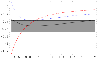
(a) $N_{B}$, $N_{EJ}$ and $N_{GLS}$ with $n_{f}=0$.

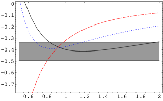
(b) $N_{B}$ with $n_{f}=3$.

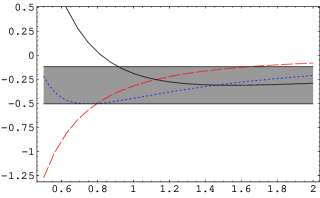
(c) $N_{B}$ with $n_{f}=6$.

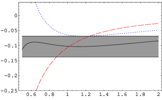
(d) $N_{EJ}$ with $n_{f}=3$.

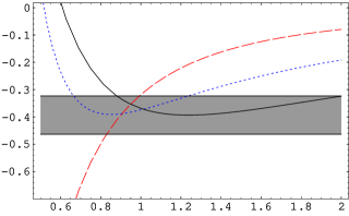
(e) $N_{GLS}$ with $n_{f}=3$.

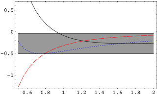
(f) $N_{GLS}$ with $n_{f}=6$.

Figure 1: Scale dependence of $N_{X}$ with conformal mapping for $n_{f}={0,3,6}$. The dashed (red) line is the LO result, the dotted (blue) line is the NLO result and the continuous (black) line the NNLO result. The band represents the error.

We are then able to give some estimates for the coefficients of the perturbative series. We provide them in tables 2, 3, 4. We should stress that our numbers incorporate the right asymptotic behaviour, which is not the case for large-$\beta_{0}$ estimates. For the Bjorken and GLS sum rules they have been calculated in [38]. The comparison with the exact result works reasonable well for $n_{f}$ smaller than 6 for the Bjorken or GLS perturbative series. For large $n_{f}$ the comparison with the exact result gets worse. Note that for $n_{f}=6$, the normalization constant of the renormalon could be almost compatible with zero if the errors are included. This fits with the picture that the renormalon is less important when the number of flavours grows and one can reach to the point where the infrared renormalon disappears. For the Ellis-Jaffe perturbative series the same discussion applies with $n_{f}$ smaller than 4 (for $n_{f}=4$ no stable determination of the normalization constant can be obtained). Again this fit with the picture that the infrared renormalon becomes weaker when the number of active flavours increase.

We can also compare with other estimates one may find in the literature for the Bjorken (GLS) sum rules [39, 40, 35, 37]. We find that our predictions somewhat lie on the upper limit of the range of values obtained in these references for $C_{B/GLS}^{(3)}$.

As a final comment it should be mentioned that the introduction of the leading logarithms in the renormalon, which is novel, does not actually improve the agreement with the running on $\nu$ of the perturbative coefficients of the perturbative series, when they are known. If this is an artifact of the leading-order analysis and would be solved at higher orders remains to be seen.

$n_{f}$	0	1	2	3	4	5	6
-$C_{B}^{(0)}(Q)$	$0.523$	$0.487$	$0.451$	$0.414$	$0.378$	$0.343$	$0.311$
-$C_{B}^{(1)}(Q)$	$0.516$	$0.452$	$0.391$	$0.334$	$0.280$	$0.228$	$0.175$
-$C_{B}^{(2)}(Q)$	$1.295$	$1.045$	$0.824$	$0.630$	$0.461$	$0.318$	$0.198$
-$C_{B}^{(3)}(Q)$	$4.199$	$3.149$	$2.285$	$1.588$	$1.042$	$0.630$	$0.334$
-$C_{B}^{(4)}(Q)$	$17.07$	$11.94$	$8.008$	$5.097$	$3.023$	$1.625$	$0.750$
-$C_{B}^{(5)}(Q)$	$83.91$	$54.77$	$34.08$	$19.93$	$10.75$	$5.175$	$2.100$

Table 2: Renormalon-based estimates of the perturbative coefficients $C_{B}^{(s)}$ for $\nu=Q$ and for different number of flavours. We use the expression from Eq. (25) except for $C_{B}^{(0)}$ for which we use the expression from Eq. (24), otherwise the result is 0.

$n_{f}$	1	2	3
-$C_{EJ}^{(0)}(Q)$	$0.423$	$0.291$	$0.103$
-$C_{EJ}^{(1)}(Q)$	$0.392$	$0.250$	$0.080$
-$C_{EJ}^{(2)}(Q)$	$0.868$	$0.478$	$0.129$
-$C_{EJ}^{(3)}(Q)$	$2.547$	$1.253$	$0.298$
-$C_{EJ}^{(4)}(Q)$	$9.476$	$4.222$	$0.896$
-$C_{EJ}^{(5)}(Q)$	$42.87$	$17.42$	$3.336$

Table 3: Renormalon-based estimates of the perturbative coefficients $C_{EJ}^{(s)}$ for $\nu=Q$ and for different number of flavours. We do not display the column with $n_{f}=0$ since the numbers are equal to the Bjorken case. We use the expression from Eq. (25) except for $C_{EJ}^{(0)}$ for which we use the expression from Eq. (24), otherwise the result is 0.

$n_{f}$	1	2	3	4	5	6
-$C_{GLS}^{(0)}(Q)$	$0.479$	$0.436$	$0.393$	$0.351$	$0.311$	$0.272$
-$C_{GLS}^{(1)}(Q)$	$0.449$	$0.379$	$0.317$	$0.260$	$0.206$	$0.154$
-$C_{GLS}^{(2)}(Q)$	$1.029$	$0.797$	$0.598$	$0.428$	$0.288$	$0.174$
-$C_{GLS}^{(3)}(Q)$	$3.100$	$2.211$	$1.507$	$0.967$	$0.569$	$0.293$
-$C_{GLS}^{(4)}(Q)$	$11.75$	$7.750$	$4.838$	$2.807$	$1.469$	$0.658$
-$C_{GLS}^{(5)}(Q)$	$53.92$	$32.97$	$18.92$	$9.980$	$4.680$	$1.841$

Table 4: Renormalon-based estimates of the perturbative coefficients $C_{GLS}^{(s)}$ for $\nu=Q$ and for different number of flavours. We do not display the column with $n_{f}=0$ since the numbers are equal to the Bjorken case. We use the expression from Eq. (25) except for $C_{GLS}^{(0)}$ for which we use the expression from Eq. (24), otherwise the result is 0.

4 Renormalon subtracted scheme

In the previous section we have obtained the contribution to the perturbative series of the leading-twist Wilson coefficient that produces its leading asymptotic behaviour. This behaviour limits the accuracy that can be obtained for the observable from the perturbative series alone, which it will always have an error of the order of the higher twist corrections. Therefore, one can not obtain these higher-twist corrections unless the perturbative series is defined with power-like accuracy. The specific value for the higher twist will depend upon the specific prescription used. Here we will adapt the procedure used in Refs. [12, 13, 14]. In those references the non-analytic behaviour in the Borel plane that produced the asymptotic behaviour of the perturbative series was subtracted from the perturbative series and added to the subleading non-perturbative contributions. Actually the definition of the non-analytic piece is ambiguous and analytic terms can always be added. The specific quantity we will substract to the perturbative series will be Eq. (27) with $n^{*}=1$. This quantity fulfils the requirement that its imaginary part cancels the imaginary part of the perturbative series and that its dependence on $Q$ complies with the structure of the higher twist contribution. For illustration, the Bjorken sum rule would read

$$M_{1}^{p}(Q^{2})-M_{1}^{n}(Q^{2})={g_{A}\over 6}C_{B,\rm RS}(Q;\nu_{f})-{4\over 27}{1\over Q^{2}}f_{3,\rm RS}(\nu_{f})\left[{\alpha_{\rm s}(\nu_{f}^{2})\over\alpha_{\rm s}(Q^{2})}\right]^{-\gamma_{\rm NS}^{0}\over 2\beta_{0}}\left(1+{\cal O}(\alpha_{\rm s})\right)+{\cal O}\left({1\over Q^{4}}\right)\,,$$ (31)

where

$$C_{B,\rm RS}(Q;\nu_{f})=C_{B}(Q)-\delta C_{B,\rm RS}(\nu_{f})=1+\sum_{s=0}^{\infty}C_{B,\rm RS}^{(s)}(Q/\nu;\nu_{f}/\nu)\alpha_{\rm s}^{s+1}(\nu)\,,$$ (32)

and

$$f_{3,\rm RS}(\nu_{f})=f_{3}(\nu_{f})-{9\over 8}Q^{2}g_{A}\left[{\alpha_{\rm s}(Q)\over\alpha_{\rm s}(\nu_{f})}\right]^{-\gamma_{\rm NS}^{0}\over 2\beta_{0}}\delta C_{B,\rm RS}(Q;\nu_{f})\,.$$ (33)

Similar changes would apply to the Ellis-Jaffe and GLS sum rules. In Eq. (32) and Eq. (33), we have subtracted and added the contributions coming from the first infrared renormalon at the scale $\nu_{f}$ respectively. Thus, in this scheme, the Wilson coefficient $C_{B,\rm RS}(Q;\nu_{f})$ is free of the first infrared renormalon and the associated $n!$ behaviour. Therefore, the series is expected to converge better. On the other hand, the higher twist, $f_{3,RS}(\nu_{f})$, is free of the first ultraviolet renormalon.

In principle, the above series could be improved by incorporating the running in $\nu_{f}$ to any order in $\alpha_{\rm s}$, which is renormalon free and therefore it could be obtained with good accuracy. In this situation it is legitimate to use the principal value (PV) prescription (or any other), since the renormalon ambiguity will cancel in the ratio. In this situation $\delta C_{X,\rm RS}$ reads

$$\delta C_{X,\rm RS}^{(PV)}(Q;\nu_{f})=\left(\alpha_{\rm s}(Q)\over\alpha_{\rm s}(\nu_{f})\right)^{-b_{X}}{\nu_{f}^{2}\over Q^{2}}N_{X}\alpha_{\rm s}(\nu_{f})\left[D_{b+b_{X}}\left(-{4\pi\over\beta_{0}\alpha_{\rm s}(\nu_{f})}\right)-1\right]$$ (34)

where

$$D_{b}(-x)=-xe^{-x}\left\{x^{b}\cos(\pi b)\Gamma(-b)-(-x)^{b}\left[\Gamma(-b)-\Gamma(-b,-x)\right]\right\}\,,$$ (35)

and,

$$\Gamma(b,x)=\int_{x}^{\infty}\!dt\,t^{b-1}e^{-t}\,,$$ (36)

denotes the incomplete $\Gamma$ function. One would then work with the following quantity

$$C_{B,\rm RS}(Q;\nu_{f})=C_{B,\rm RS}(Q;\nu)+\left[\delta C_{X,\rm RS}^{(PV)}(Q;\nu)-\delta C_{X,\rm RS}^{(PV)}(Q;\nu_{f})\right]\,,$$ (37)

where one would set $\nu\sim Q$ and work order by order in perturbation theory in the first term in the right-hand side (where there is no large logs), whereas for the other terms the PV prescription is used. This allows to partially resum the dependence on $\nu_{f}$. Let us also note that the first term in Eq. (35) corresponds to $\Lambda_{\overline{\rm MS}}$ (up to the anomalous dimension). Therefore it cancels in the difference, $\delta C_{X,\rm RS}^{(PV)}(Q;\nu)-\delta C_{X,\rm RS}^{(PV)}(Q;\nu_{f})$, and can be neglected. Working with the principal value prescription has produced very good results in heavy quark physics, where it was possible to check the running of $\nu_{f}$ with ”experiment” (lattice), see [14]. However, in that situation, the running in $\nu_{f}$ was known with a very high accuracy, since there was no anomalous dimension and the running on $\nu_{f}$ could be deduced simply from the running of $\alpha_{\rm s}$. In our case we only know the leading order and we expect a less accurate result.

Finally, we would like to mention that our knowledge of the running in $\nu$ of the higher twist terms is much more limited than in heavy quark physics. Here, we only know the leading log running. This has consequences in Eq. (32) since, once we expand in $\alpha_{\rm s}(\nu)$, there are some subleading logs which are unknown.

5 Comparison with experiment

In this section we will compare our theoretical predictions with the experimental data. Our aim is to perform a combined global fit for the three sum rules. We will use the experimental data for the Bjorken sum rule from [41, 42, 43, 44, 28] analyzed according to Ref. [28]. Note that the elastic contribution has to be included in the experimental numbers in order the sum rule to be fully inclusive, i.e.

$$\Gamma(Q^{2})={1\over 2}F_{1}(Q^{2})\left(F_{1}(Q^{2})+F_{2}(Q^{2})\right)+\Gamma_{\rm inel.}(Q^{2})\,.$$ (38)

The empirical parameterization of the elastic form factors was taken from [45]. For large momentum this contribution is completely negligible.

We take the experimental data points for $M_{1}^{p}(Q^{2})$ from Ref. [27], which have used the experimental results for the structure functions from [46, 47, 48, 49, 50, 51, 52, 53].

For the GLS sum rule we will use the experimental data from the CCFR collaboration [30].

We first illustrate the problem of convergence of the perturbative series by drawing the perturbative series in the $\overline{\rm MS}$ scheme at different orders in $\alpha_{\rm s}$ in Fig. 2.

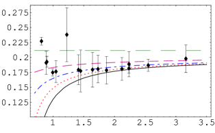
(a) Bjorken Sum Rule.

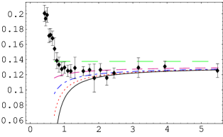
(b) Ellis-Jaffe Sum Rule.

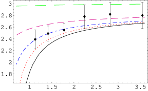
(c) GLS Sum Rule.

Figure 2: Leading-twist contribution to the sum rules at different orders in perturbation theory in the $\overline{\rm MS}$ scheme with $\nu=Q$ compared with the experimental data. The long-dashed (green) line is the LO result. The dashed (magenta) line is the NLO result. The dot-dashed (blue) line is the NNLO result. The dotted (red) line is the NNNLO result and the continuous black line is the (estimate) N⁴LO^∗. At this order we have used a renormalon-based estimate for $C_{X}^{(3)}(Q)$ from Tables 2, 3, 4. ${\hat{a}}_{0}=0.141$.

The perturbative series has a relative good convergence. However, this convergence deteriorates when we approach to low energies. We also see how the perturbative theoretical result diverges from the experimental numbers at low energies. As we have already stated, the solution to this problem comes from using the RS scheme. We plot again the perturbative series in the RS scheme in Fig. 3 for two values of $\nu_{f}$: $\nu_{f}=0.8$ and 1 GeV.

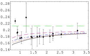
(a) $\nu_{f}=0.8$.

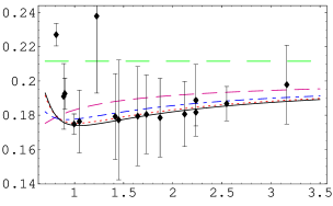
(b) $\nu_{f}=1$.

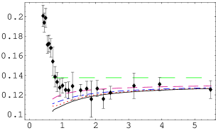
(c) $\nu_{f}=0.8$.

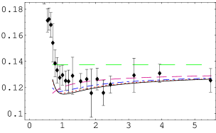
(d) $\nu_{f}=1$.

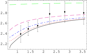
(e) $\nu_{f}=0.8$.

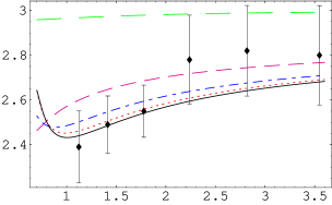
(f) $\nu_{f}=1$.

Figure 3: Leading-twist contribution to the sum rules at different orders in perturbation theory in the $\rm RS$ scheme with $\nu=Q$ for two different values of the subtraction point, $\nu_{f}$, compared with the experimental data. The long-dashed (green) line is the LO result. The dashed (magenta) line is the NLO result. The dot-dashed (blue) line is the NNLO result. The dotted (red) line is the NNNLO result and the continuous black line is the (estimate) N⁴LO^∗. At this order we have used a renormalon-based estimate for $C_{X}^{(3)}(Q)$ from Tables 2, 3, 4. ${\hat{a}}_{0}=0.141$.

We can see that in both cases the convergence of the perturbative series improves. This is specially so around the 1 GeV region. For $\nu_{f}=1$ GeV we can also see a qualitative change in the figure with a much better agreement with experiment around the 1 GeV region. This alone does not mean much, since it only reflects the $\nu_{f}$ scale dependence of the pure perturbative piece. Nevertheless, this scale dependence is known and can be predicted by perturbation theory. This scale dependence cancels with the scale dependence of the higher-twist terms. Therefore, the complete result, including the higher twist terms, should be independent of $\nu_{f}$. Thus, consistency demands that if we perform the fit to experiment including the higher twist $f_{i}(\nu_{f})$ for different values of $\nu_{f}$, in particular for 0.8 and 1 GeV, the results obtained for the $f_{i}(\nu_{f})$ should be consistent with the result obtained by performing the perturbative running in $\nu_{f}$ with respect these two values. We have checked that this is so within the errors of our evaluation. This reassures the reliability of our fit. This also tells us that it is reasonable to use the operator product expansion formulas for $Q$ larger than 0.8 GeV. This is the attitude we will take in this paper where we will include (unless otherwise indicated) the experimental points for $Q>0.8$ GeV. Therefore, the perturbative plots in Fig. 3 with $\nu_{f}=1$ GeV can be reinterpreted as that a piece of the higher twist correction has been included in the pure perturbative term. This piece corresponds to the running of $\nu_{f}$ from 0.8 to 1 GeV of the higher twist term and can be obtained from the renormalization group. Therefore, in this sense, the change of slope observed in Fig. 3 can be interpreted as having its origin in perturbation theory. Note that the change of slope, from the experimental point of view, comes from the elastic term.

In Fig. 3 higher-twist effects have not been included. Our next aim is to perform a fit of ${\hat{a}}_{0}$ and the subleading twist matrix elements from the available experimental data. We refrain from trying to fit $\alpha_{\rm s}$, since the experimental errors appear to be too large. Actually, they will be one of the major source of uncertainty of our analysis. We perform a global fit of all the available data from the different sum rules at the same time. The size of the experimental errors is the largest for the GLS sum rule, whereas the most accurate data come from the $M_{1}^{p}(Q^{2})$ experimental points. In any case, $f_{5}^{S}$ will be obtained from the GLS sum rule alone, since this fit is independent of the other two sum rules. We perform the global fit to different orders in the expansion in $\alpha_{\rm s}$ of the leading twist perturbative Wilson coefficient. We work with the running $\alpha_{\rm s}$ consistent with the accuracy one is working at each order. We show the results of the fit at different orders in perturbation theory in Table 5. We can see how the series shows convergence. We can then obtain relatively good estimates for ${\hat{a}}_{0}$ and $f_{3}$, for the other non-perturbative parameters the situation is less conclusive. The values have been obtained with $\nu_{f}=1$ GeV.

	${\hat{a}}_{0}$	$f_{0,\rm RS}$ (1 GeV)	$f_{3,\rm RS}$ (1 GeV)	$f_{5,\rm RS}^{S}$ (1 GeV)	$f_{8,\rm RS}$ (1 GeV)
LO	$0.043$	$-1.571$	$0.119$	$1.030$	$5.90$
NLO	$0.120$	$-0.817$	$-0.075$	$0.304$	$3.11$
NNLO	$0.136$	$0.014$	$-0.106$	$0.097$	$-0.18$
NNNLO	$0.139$	$0.552$	$-0.117$	$0.014$	$-2.34$
N4LO∗	$0.141$	$0.790$	$-0.124$	$-0.029$	$-3.30$

Table 5: Determination of ${\hat{a}}_{0}$ and the higher-twist non-perturbative parameters from the global fit to the sum rules at different orders in perturbation theory.

In order to estimate the errors, we allow for a variation of $\alpha_{\rm s}(M_{z})=0.118\pm 0.003$, of $N_{X}$ (according to the error given in Table 1), of the allowed set of experimental points (we consider two situations: a) all the data points for $q>0.8$ GeV and b) all the data points for $q>1$ GeV; our central values will be the ones obtained with option a)), and also consider the experimental errors. We also consider the difference between the N³LO^∗ and NNLO result as an estimate of the error due to the convergence of the series. This error happens to be very small in comparison with the other source of errors. Summarizing, we obtain (with the $f_{i}$ in units of GeV²)

$${\hat{a}}_{0} = 0.141^{+0.006}_{-0.004}(\delta\alpha_{\rm s}){}^{+0.002}_{-0.002}(\delta N_{X}){}^{+0.088}_{-0.088}({\exp}){}^{+0.001}_{-0.001}({\rm pert}){}^{+0.010}_{-0.010}(q>1)\,,$$ (39)

$$f_{0,\rm RS}(1\;{\rm GeV}) = 0.790^{+0.241}_{-0.399}(\delta\alpha_{\rm s}){}^{-0.489}_{+0.489}(\delta N_{X}){}^{+0.159}_{-0.159}({\exp}){}^{+0.238}_{-0.238}({\rm pert}){}^{+1.060}_{-1.060}(q>1)\,,$$ (40)

$$f_{3,\rm RS}(1\;{\rm GeV}) = -0.124^{-0.050}_{+0.032}(\delta\alpha_{\rm s}){}^{-0.049}_{+0.049}(\delta N_{X}){}^{-0.121}_{+0.121}({\exp}){}^{+0.007}_{-0.007}({\rm pert}){}^{+0.026}_{-0.026}(q>1)\,,$$ (41)

$$f_{5,\rm RS}^{S}(1\;{\rm GeV}) = -0.029^{-0.162}_{+0.124}(\delta\alpha_{\rm s}){}^{-0.065}_{+0.065}(\delta N_{X}){}^{-0.344}_{+0.344}({\exp}){}^{+0.042}_{-0.042}({\rm pert})\pm 0(q>1)\,,$$ (42)

$$f_{8,\rm RS}(1\;{\rm GeV}) = -3.30^{-0.98}_{+1.61}(\delta\alpha_{\rm s}){}^{+1.95}_{-1.95}(\delta N_{X}){}^{-0.27}_{+0.27}({\exp}){}^{+0.96}_{-0.96}({\rm pert}){}^{+4.27}_{-4.27}(q>1)\,.$$ (43)

If we combine all the errors in quadrature we obtain

$${\hat{a}}_{0} = 0.141\pm 0.089\,,$$ (44)

$$f_{0,\rm RS}(1\;{\rm GeV}) = 0.790^{+1.225}_{-1.266}\;{\rm GeV}^{2}\,,$$ (45)

$$f_{3,\rm RS}(1\;{\rm GeV}) = -0.124^{+0.137}_{-0.142}\;{\rm GeV}^{2}\,,$$ (46)

$$f_{5,\rm RS}^{S}(1\;{\rm GeV}) = -0.029^{+0.374}_{-0.388}\;{\rm GeV}^{2}\,,$$ (47)

$$f_{8,\rm RS}(1\;{\rm GeV}) = -3.30^{+5.06}_{-4.90}\;{\rm GeV}^{2}\,,$$ (48)

We have also performed the fit with $\nu_{f}=0.8$. We obtain in this case

$${\hat{a}}_{0} = 0.143\,,$$ (49)

$$f_{0,\rm RS}(0.8\;{\rm GeV}) = 0.365\,,$$ (50)

$$f_{3,\rm RS}(0.8\;{\rm GeV}) = -0.210\,,$$ (51)

$$f_{5,\rm RS}^{S}(0.8\;{\rm GeV}) = -0.167\,,$$ (52)

$$f_{8,\rm RS}(0.8\;{\rm GeV}) = -1.58\,,$$ (53)

whereas the magnitude of the errors is similar to the fit with $\nu_{f}=1$ GeV. As expected, the value of ${\hat{a}}_{0}$ almost remain independent of $\nu_{f}$. The higher twist parameters do depend on $\nu_{f}$ in a way predicted by the renormalization group. For instance, for $f_{3}$ we would have the following expression

$$f_{3,\rm RS}(\nu_{f})=f_{3,\rm RS}(\nu_{f}^{\prime})\left[{\alpha_{\rm s}(\nu_{f}^{\prime})\over\alpha_{\rm s}(\nu_{f})}\right]^{-\gamma_{\rm NS}^{0}\over 2\beta_{0}}+{9\over 8}\nu_{f}^{2}g_{A}\left[\delta C_{B,\rm RS}(Q=\nu_{f};\nu_{f}^{\prime})-\delta C_{B,\rm RS}(Q=\nu_{f};\nu_{f})\right]$$ (54)

and analogously for the other higher twist terms. Therefore, we should recover the values in Eqs. (44-48) after performing the renormalization group running of Eqs. (50-53). If we perform such running we obtain

$$f_{0,\rm RS}(1\;{\rm GeV}) = 0.335\,{\rm GeV}^{2},$$ (55)

$$f_{3,\rm RS}(1\;{\rm GeV}) = -0.130\,{\rm GeV}^{2},$$ (56)

$$f_{5,\rm RS}^{S}(1\;{\rm GeV}) = -0.004\,{\rm GeV}^{2},$$ (57)

$$f_{8,\rm RS}(1\;{\rm GeV}) = -1.46\,{\rm GeV}^{2}\,.$$ (58)

We see that the running goes in the right direction for $f_{3}$ and $f_{5}^{S}$, whereas for $f_{0}$ and $f_{8}$ the values remain constant. Either way, the numbers agree with those obtained in Eqs. (45-48) within errors.

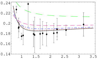
(a) Bjorken Sum Rule.

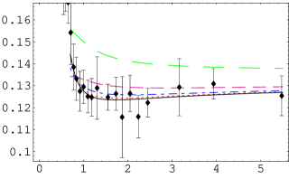
(b) Ellis-Jaffe Sum Rule.

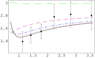
(c) GLS Sum Rule.

Figure 4: Global fit to the Sum Rules in the RS scheme with $\nu=Q$ at different orders in perturbation theory including the leading and next-to-leading twist term. The long-dashed (green) line is the LO result. The dashed (magenta) line is the NLO result. The dot-dashed (blue) line is the NNLO result. The dotted (red) line is the NNNLO result and the continuous black line is the (estimate) N⁴LO^∗. At this order we have used a renormalon-based estimate for $C_{X}^{(3)}(Q)$ from Tables 2, 3, 4. The values of ${\hat{a}}_{0}$, $f_{i}$ and $f_{5}^{S}$ are taken from Eqs. (44-48).

Finally, we have also considered the inclusion of $1/Q^{4}$ corrections. The values of $f_{0}$ and $f_{8}$ are not stable under the inclusion of these effects, although there is a correlation on the values of $f_{0}$ and $f_{8}$: a large positive value of $f_{0}$ is only possible if we also have a large negative value of $f_{8}$. The point is that, even if formally it should be possible to distinguish $f_{0}$ and $f_{8}$ due to the different anomalous dimension, in practice we do not have enough accuracy. Therefore, the values obtained above for $f_{0}$ and $f_{8}$ (and its errors) should be taken with caution. This warning also applies to the determination of $f_{5}^{S}$, for which the inclusion of $1/Q^{4}$ corrections significantly changes its value. For the other coefficients, ${\hat{a}}_{0}$ and $f_{3}$ the variations are smaller than the errors of our fit.

The error appears to be dominated by the experimental one in ${\hat{a}}_{0}$ and $f_{3}$, the objects we can compute with better accuracy.

We would also like to note that, in some cases, the values of the higher-twist non-perturbative parameters are compatible with zero within errors.

To illustrate the quality of the fit we plot our final results, the sum rules including the leading and subleading twist, at different orders in perturbation theory with our best fit, Eqs. (44-48), compared with the experimental data in Fig. 4.

The analysis of the GLS sum rule taking into account renormalon effects has been considered in Ref. [37]. In this reference only two data points were used and a Principal Value-like Borel resummation prescription was used. The authors also included some pure non-perturbative effects arguing that they could be inherited from the renormalon computation. This is still an open question and, actually, it has been criticised by one of the authors in Ref. [54].

6 Conclusions

We have studied the large order behaviour in perturbation theory of the Bjorken, Ellis-Jaffe and GLS sum rules. In particular, we have considered their first infrared renormalons, for which we have obtained their analytic structure with logarithmic accuracy and also an approximate determination of their normalization constant. Estimates of higher order terms of the perturbative series are given. The RS scheme has been worked out for these observables and compared with experimental data. The convergence of the perturbative series greatly improves in this scheme, specially around the 1 GeV region. In particular, for $\nu_{f}=1$ GeV, the agreement between the pure perturbative contribution and experiment is quite good. The fact that we have a convergent series in perturbation theory allows to give meaningful values for the higher twist condensates with well defined errors. We have performed a detailed analysis, being able to give predictions for ${\hat{a}}_{0}$ and some higher twist condensates, including error bars. Our best fits for the sum rules can be found in Fig. 4. The values for the non-perturbative matrix elements read

$${\hat{a}}_{0} = 0.141\pm 0.089\,,$$ (59)

$$f_{3,\rm RS}(1\;{\rm GeV}) = -0.124^{+0.137}_{-0.142}\,{\rm GeV}^{2}\,.$$ (60)

The experimental situation is not very good for the GLS sum rule, for which we can not give a precise number for the higher twist. The experimental precision is not good enough to check the assumption of [55] that $f_{3}$ and $f_{5}^{S}$ are equal. We also do not display here the values of $f_{0}$ and $f_{8}$, since they have large errors and their values in the fit are somewhat correlated. A large value of one of them could be obtained in the fit to the price of having the other being large with opposite sign.

One of the most important source of error of the present analysis is the experimental one. Any improvement in this respect will immediately lead to a reduction of the errors of the numbers obtained in this paper.

The quality of the analysis is worse than the one obtained for heavy quark physics analysis. The sensitivity to the renormalon is smaller and the determination of the normalization constant is less accurate that in that case. This was to be expected since the singularities in the Borel plane are more far away here than in heavy quark physics. In any case, the inclusion of the renormalon cancellation introduces a qualitative change on the perturbative behaviour around the 1 GeV region making it much closer to the experimental figures.

Another issue we would like to mention is that the resummation of renormalon-related logarithms does not appear to improve the convergence of the series. On the other hand, we have only performed the leading log resummation in this paper. It would be interesting to see what happens at higher orders.

Finally, the possibility to merge with the chiral limit seems closer now but the gap still exists. In particular one should find a systematic way to incorporate higher twist effects.

Acknowledgments.
We would like to thank A. Deur and M. Osipenko for providing detailed information on the experimental points of Refs. [28] and [27] respectively. F.C. acknowledges support of the Natural Sciences and Engineering Research Council of Canada. A.P. is supported by MCyT and Feder (Spain), FPA 2004-04582-C02-01 and by CIRIT (Catalonia), 2001SGR-00065.

References

- [1]
- [2] D.J. Gross, C.H. Llewellyn Smith, Nucl. Phys. B 14, 337 (1969).
- [3] J. D. Bjorken, Phys. Rev. 148, 1467 (1966).
- [4] J. Ellis, R.L. Jaffe, Phys. Rev D 9, 1444 (1974), E-ibid 10, 1669 (1974).
- [5] G. ’t Hooft, in The Whys of Subnuclear Physics, edited by A. Zichichi (Plenum, New York, 1978).
- [6] G. Parisi, Phys. Lett. B 76, 65 (1978).
- [7] A. H. Mueller, Phys. Lett. B 308, 355 (1993).
- [8] I. I. Y. Bigi, M. A. Shifman, N. G. Uraltsev and A. I. Vainshtein, Phys. Rev. D 50, 2234 (1994) [arXiv:hep-ph/9402360].
- [9] M. Neubert, C.T. Sachrajda, Nucl. Phys. B 438, 235 (1995).
- [10] M.E. Luke, A.V. Manohar, M.J. Savage, Phys. Rev. D 51, 4924 (1995).
- [11] M. Beneke, Phys. Lett. B 344, 341 (1995).
- [12] A. Pineda, JHEP 0106, 022 (2001) [arXiv:hep-ph/0105008].
- [13] A. Pineda, J. Phys. G 29, 371 (2003) [arXiv:hep-ph/0208031].
- [14] G. S. Bali and A. Pineda, Phys. Rev. D 69, 094001 (2004) [arXiv:hep-ph/0310130].
-
[15]
J. Kodaira, S. Matsuda, T. Muta, K. Sasaki, T. Uematsu,
Phys. Rev. D 20 (1979) 627;
J. Kodaira, S. Matsuda, K. Sasaki, T. Uematsu, Nucl. Phys. B 159 (1979) 99. - [16] S.G. Gorishny, S.A. Larin, Phys. Lett. B 172 (1986) 109.
- [17] S.A. Larin, J.A.M. Vermaseren, Phys. Lett. B 259 (1991) 345.
- [18] V.M. Braun, A.V. Kolesnichenko, Nucl. Phys. B 283 (1987) 723.
- [19] J. Kodaira, Nucl. Phys. B 165 (1980) 129.
- [20] S.A. Larin, Phys. Lett. B 334 (1994) 192.
- [21] S. A. Larin, T. van Ritbergen and J. A. M. Vermaseren, Phys. Lett. B 404, 153 (1997) [arXiv:hep-ph/9702435].
- [22] I.I. Balitsky, V.M. Braun, A.V. Kolesnichenko, Phys. Lett. B 242 (1990) 245; E-ibid B 318 (1993) 648.
- [23] H. Kawamura, T. Uematsu, J. Kodaira and Y. Yasui, Mod. Phys. Lett. A 12, 135 (1997) [arXiv:hep-ph/9603338].
- [24] S. Eidelman et al. [Particle Data Group], Phys. Lett. B 592, 1 (2004).
- [25] P. G. Ratcliffe, Czech. J. Phys. 54, B11 (2004) [arXiv:hep-ph/0402063].
- [26] O. Nachtmann, Nucl. Phys. B 63, 237 (1973).
- [27] M. Osipenko et al., Phys. Rev. D 71, 054007 (2005) [arXiv:hep-ph/0503018].
- [28] A. Deur et al., Phys. Rev. Lett. 93, 212001 (2004) [arXiv:hep-ex/0407007].
- [29] I. Hinchliffe and A. Kwiatkowski, Ann. Rev. Nucl. Part. Sci. 46, 609 (1996) [arXiv:hep-ph/9604210].
- [30] J. H. Kim et al., Phys. Rev. Lett. 81, 3595 (1998) [arXiv:hep-ex/9808015].
- [31] J. Blumlein and W. L. van Neerven, Phys. Lett. B 450, 417 (1999) [arXiv:hep-ph/9811351].
- [32] A.G. Grozin, M. Neubert, Nucl. Phys. B 508, 311 (1997).
- [33] F. Campanario, A.G. Grozin, T. Mannel, Nucl. Phys. B 663, 280 (2003); E-ibid. B 670, 331 (2003) [arXiv:hep-ph/0303052].
- [34] M. Beneke, V. M. Braun and N. Kivel, Phys. Lett. B 404, 315 (1997) [arXiv:hep-ph/9703389].
- [35] J. R. Ellis, E. Gardi, M. Karliner and M. A. Samuel, Phys. Lett. B 366, 268 (1996) [arXiv:hep-ph/9509312].
- [36] T. Lee, Phys. Rev. D 56, 1091 (1997) [arXiv:hep-th/9611010]; Phys. Lett. B 462, 1 (1999) [arXiv:hep-ph/9908225].
- [37] C. Contreras, G. Cvetic, K. S. Jeong and T. Lee, Phys. Rev. D 66, 054006 (2002) [arXiv:hep-ph/0203201].
- [38] D. J. Broadhurst and A. L. Kataev, Phys. Lett. B 315, 179 (1993) [arXiv:hep-ph/9308274].
- [39] A. L. Kataev, Phys. Rev. D 50, 5469 (1994) [arXiv:hep-ph/9408248].
- [40] A. L. Kataev and V. V. Starshenko, Mod. Phys. Lett. A 10, 235 (1995) [arXiv:hep-ph/9502348].
- [41] K. Abe et al. [E143 collaboration], Phys. Rev. D 58, 112003 (1998) [arXiv:hep-ph/9802357].
- [42] B. Adeva et al. [Spin Muon Collaboration], Phys. Rev. D 58, 112002 (1998).
- [43] P. L. Anthony et al. [E155 Collaboration], Phys. Lett. B 493, 19 (2000) [arXiv:hep-ph/0007248].
- [44] A. Airapetian et al. [HERMES Collaboration], Eur. Phys. J. C 26, 527 (2003) [arXiv:hep-ex/0210047].
- [45] P. Mergell, U. G. Meissner and D. Drechsel, Nucl. Phys. A 596, 367 (1996) [arXiv:hep-ph/9506375].
- [46] M. J. Alguard et al., Phys. Rev. Lett. 37, 1261 (1976); ibid 41, 70 (1978).
- [47] G. Baum et al., Phys. Rev. Lett. 45, 2000 (1980).
- [48] K. Abe et al., Phys. Rev. D 58, 112003 (1998).
- [49] P. L. Anthony et al., Phys. Lett. B 493, 19 (2000).
- [50] J. Ashman et al., Nucl. Phys. B328, 1 (1989).
- [51] B. Adeva et al., Phys. Rev. D 58, 112001 (1998); B. Adeva et al., Phys. Rev. D 60, 072004 (1999); Erratum ibid. D 62, 079902 (2000).
- [52] A. Airapetian et al., Phys. Lett. B 442, 484 (1998).
- [53] R. Fatemi et al., Phys. Rev. Lett. 91, 222002 (2003).
- [54] G. Cvetic, Phys. Rev. D 67, 074022 (2003) [arXiv:hep-ph/0211226].
- [55] A. L. Kataev, JETP Lett. 81, 608 (2005) [Pisma Zh. Eksp. Teor. Fiz. 81, 744 (2005)] [arXiv:hep-ph/0505108].