x Constraint equations for heavy-to-light currents in SCET

Abstract

A complete basis for the next-to-next-to leading order heavy-to-light currents in the soft-collinear effective theory is constructed. Reparameterization invariance is imposed by deriving constraint equations. Their solutions give the set of allowed Dirac structures as well as relations between the Wilson coefficients of operators that appear at different orders in the power expansion. The completeness of reparameterization invariance constraints derived on a projected surface is investigated. We also discuss the universality of the ultrasoft Wilson line with boundary conditions.

I Introduction

The soft-collinear effective theory (SCET) provides a systematic approach for separating hard, soft, and collinear dynamics in processes with energetic quarks and gluons Bauer et al. (2001a, b); Bauer and Stewart (2001); Bauer et al. (2002a). In SCET the infrared physics is described by effective theory fields with well defined momentum scaling, which are used to build operators order by order in the power expansion. The hard perturbative corrections are contained in the Wilson coefficients which can be computed by matching computations order by order in perturbation theory in $\alpha_{s}$. The symmetries and power counting in the effective theory simplify the derivation of factorization theorems and provide a systematic method of treating power suppressed contributions. The construction of the complete set of allowed operators for a process is one of the first steps towards deriving factorization theorems. The operators are constrained by gauge symmetry in the effective theory, as well as by heavy quark effective theory (HQET) and SCET reparameterization invariance (RPI) Luke and Manohar (1992); Chay and Kim (2002); Manohar et al. (2002). The operators and Wilson coefficients are typically coupled by a convolution integral over the large momenta of gauge invariant products of collinear fields. In some cases perturbative matching computations are not necessary, since RPI gives relations between Wilson coefficients that are valid to all orders in perturbation theory.

Heavy-to-light currents, $J=\bar{q}\Gamma b$, are important for describing a broad range of processes with SCET, including both inclusive semileptonic and radiative decays like $B\to X_{u}\ell\bar{\nu}$ and $B\to X_{s}\gamma$ Bauer et al. (2001a, b, 2002a); Bauer and Manohar (2004); Bosch et al. (2004a); Lee and Stewart (2005); Bosch et al. (2004b); Beneke et al. (2005); Lange et al. (2005); Chay et al. (2005a), exclusive semileptonic and radiative decays such as $B\to\pi\ell\bar{\nu}$ and $B\to K^{*}\gamma$ Bauer et al. (2001b); Chay and Kim (2002); Beneke et al. (2002); Bauer et al. (2003a); Pirjol and Stewart (2003); Chay and Kim (2003); Beneke and Feldmann (2004); Lange and Neubert (2004); Grinstein et al. (2005); Becher et al. (2005), and exclusive hadronic decays like $B\to\pi\pi$ Chay and Kim (2004); Bauer et al. (2004a); Beneke et al. (1999); Feldmann and Hurth (2004).

Here we will consider higher order RPI relations for heavy-to-light currents in a theory $\textrm{SCET}_{\textrm{I}}\$with ultrasoft (usoft) and collinear fields. Any momentum can be decomposed as $p^{\mu}=n\!\cdot\!p\>{\bar{n}}^{\mu}/2+{\bar{n}}\!\cdot\!p\>n^{\mu}/2+p_{\perp}^{\mu}$, where $n_{\mu},{\bar{n}}_{\mu}$ are two light-cone vectors satisfying $n^{2}={\bar{n}}^{2}=0$ and $n\cdot{\bar{n}}=2$. The vector $n^{\mu}$ appears as a label for the collinear quarks $\xi_{n}$ and gluons $A_{n}^{\mu}$, and the quantum fluctuations described by these fields are predominately about this direction. The collinear modes have momentum scaling as $(n\cdot p,{\bar{n}}\cdot p,p_{\perp})\sim Q(\lambda^{2},1,\lambda)$. The usoft modes $q_{us},A_{us}^{\mu}$ have momenta $p_{us}^{\mu}\sim Q\lambda^{2}$. We also use HQET usoft fields $h_{v}$ for heavy quarks, where $v^{\mu}$ is a velocity label vector with $v^{2}=1$ (see for example Manohar and Wise (2000); Neubert (1994)). The mass of the heavy quark is denoted by $m$, $Q$ is a hard energy scale $\sim m$, and $\lambda\ll 1$ is the SCET expansion parameter. The auxiliary vectors $n,\bar{n}$ and $v$ break part of the full Lorentz symmetry of QCD, and this symmetry is restored order by order in the power counting by reparameterization invariance under changes in these parameters. For processes involving heavy-to-light currents it is often convenient to work in the special frame where $v_{\perp}=0$, so that $v^{\mu}={\bar{n}}\!\cdot\!v\>n^{\mu}/2+n\!\cdot\!v\>{\bar{n}}^{\mu}/2$ and $n\!\cdot\!v\>{\bar{n}}\!\cdot\!v=1$.

In HQET it is convenient to formulate the RPI constraints Luke and Manohar (1992) to all orders in $1/m$ by constructing RPI invariant operators and then expanding them to generate a chain of related operators. These operators start at some fixed order in $1/m$, but once the RPI invariant form of this operator is known, all higher terms in the chain are determined. The RPI symmetries in SCET are richer and typically the constraints are derived order by order in $\lambda$. In this case, higher order operators in the chain are not fully determined until the appropriate order in $\lambda$ is considered.

Reparamaterization invariance constraints in SCET were first considered by Chay and Kim Chay and Kim (2002). The complete set of SCET RPI transformations were formulated in Ref. Manohar et al. (2002) and used to prove that the leading order (LO) SCET Lagrangian is not renormalized to all orders in perturbation theory. RPI constraints on subleading Lagrangians and tree level currents to ${\mathcal{O}}(\lambda^{2})$ were derived in Ref. Beneke et al. (2002) (and verified in Lee and Stewart (2005) for a basis with $v_{\perp}\neq 0$). At ${\mathcal{O}}(\lambda)$, the extension to a complete set of heavy-to-light currents constrained by RPI relations including currents that appear beyond tree-level was made in Ref. Pirjol and Stewart (2003). At this order, all Wilson coefficients are constrained by RPI except for one scalar, four vector, and six tensor currents, for which the one-loop matching was done in Ref. Beneke et al. (2004) and independently in Ref. Becher and Hill (2004). For the currents that survive for $v_{\perp}=0$ the ${\mathcal{O}}(\lambda)$, RPI relations were verified in Ref. Hill et al. (2004). To simplify the computation, they considered constraints restricted to the projected $v_{\perp}=0$ surface (from the RPI-$\star$ transformation defined later) since this involves writing down fewer operators. At ${\mathcal{O}}(\lambda^{2})$, the allowed set of field structures for the heavy-to-light currents was determined in Ref. Beneke et al. (2005). Four quark operator currents first appear at this order. Recently the type-II RPI invariance was extended to include light quark mass effects and provide constraints on certain $m_{q}$ dependent operators Chay et al. (2005a). For heavy-to-light currents at ${\cal O}(\lambda^{2})$ a complete basis of Dirac structures and the full set of RPI relations have not yet been constructed.

In constructing subleading operators we combine objects that are individually collinear and usoft gauge invariant. The logic which ensures that all subleading operators can be organized in terms of these objects relies on the decoupling of usoft gluons from the leading order collinear Lagrangian by a field redefinition involving a Wilson line $Y$ Bauer et al. (2002a). In section II.2 we show that all results are independent of the choice of boundary condition for this Wilson line. Processes described by SCET can depend on the path of Wilson lines, but this path is determined independent of the choice of boundary condition.

Our main objective in this paper is to to derive the complete basis of currents at ${\mathcal{O}}(\lambda^{2})$ by constructing a basis that is valid at any order in perturbation theory and including all RPI relations. Results are derived for use in the $v_{\perp}=0$ frame (and we take $m_{q}=0$ in all currents). Two combinations of {SCET RPI-I, SCET RPI-II, HQET RPI} are formed which leave $v_{\perp}=0$, and are called RPI-$\star$ and RPI-$ (section II.3). We call these transformations on the surface $v_{\perp}=0$ “projected RPI relations” and study their completeness in the full space of allowed transformations in section II.4. For the ${\mathcal{O}}(\lambda^{2})$ heavy-to-light currents, we show that transformations on the projected surface give the complete set of relations for currents defined on this surface (see section III.4). By eliminating the field operators we show that it is convenient to consider the RPI relations as constraint equations of the form

$$\sum_{i,k}B_{i}(\omega_{k})\ \Gamma^{B}_{i}=\sum_{j,\ell}C_{j}(\omega_{\ell})\ \Gamma^{C}_{j}\,,$$ (1)

where $B_{i}$ and $\Gamma^{B}_{i}$ are Wilson coefficients and Dirac structures for operators that appear at some fixed order in $\lambda$, and $C_{j}$ and $\Gamma^{C}_{i}$ are terms that appeared in operators from lower orders. By deriving these constraint equations in section III.2 prior to searching for their solutions, it becomes easier to simultaneously consider the restrictions imposed by the five different types of RPI invariance from both SCET and HQET, since each gives a separate constraint. A simple counting procedure is given for determining all possible Dirac structures prior to imposing the RPI conditions. The solution of the constraint equations in section III.3 give relations between the $B_{i}$ and $C_{j}$ coefficients and determine the allowed Dirac structures $\Gamma^{B}_{i}$ in terms of $\Gamma^{C}_{j}$.

II Ingredients from SCET

II.1 Degrees of freedom, power counting, gauge invariance, and Wilson lines

We briefly review some basic definitions from SCET that we will need for our computations. The fields include collinear gluons $A_{n}^{\mu}$, ultrasoft gluons $A_{us}^{\mu}$, collinear quarks $\xi_{n}$, and heavy quarks $h_{v}$. An important attribute of our collinear fields is that they carry both a large label momentum $p$ and a coordinate $x$, such as $\xi_{n,p}(x)$. The label momenta are picked out by momentum operators, $\bar{\mathcal{P}}\xi_{n,p}={\bar{n}}\!\cdot\!p\,\xi_{n,p}$ and ${\mathcal{P}}_{\perp}^{\mu}\xi_{n,p}=p_{\perp}^{\mu}\xi_{n,p}$ (see Ref. Bauer and Stewart (2001)), while derivatives $i\partial^{\mu}$ act on $x$ and scale like ultrasoft momenta. We define collinear covariant derivatives

$$i\bar{n}\cdot D_{c}=\overline{\mathcal{P}}+g\bar{n}\cdot A_{n}\,,\qquad iD_{c}^{\perp\mu}=\mathcal{P}_{\bot}^{\mu}+gA_{n}^{\perp\mu}\,,\qquad in\cdot D_{c}=in\cdot\partial+gn\cdot A_{n},$$ (2)

and an usoft covariant derivative

$$iD_{us}^{\mu}=i\partial^{\mu}+gA_{us}^{\mu}.$$ (3)

To construct gauge invariant structures, it is useful to define the collinear Wilson line

$$W \equiv \Big{[}\sum_{\textrm{perms}}\exp\Big{(}-\frac{g}{\overline{\mathcal{P}}}\>\bar{n}\cdot A_{n}\ \Big{)}\Big{]}$$ (4)

and an ultrasoft Wilson line

$$Y(x^{\mu})\equiv{\tilde{\textrm{P}}}\exp\Big{(}i\,g\int^{0}_{s_{0}}\!\!ds\ n\!\cdot\!A_{us}(x^{\mu}+sn^{\mu})\Big{)}\,,$$ (5)

where it is convenient to choose the reference point $s_{0}$ to be $s_{0}=-\infty$ with $\tilde{\textrm{P}}={\textrm{P}}$ path ordering for both quarks and antiquarks. We comment on the $s_{0}$ independence of results in the next section. Making the collinear field redefinitions Bauer et al. (2002a)

$$\xi_{n,p}(x)\to Y(x)\xi_{n,p}(x)\,,\qquad A_{n,q}(x)\to Y(x)A_{n,q}(x)Y^{\dagger}(x)\,,$$ (6)

removes all couplings to usoft gluons from the leading order collinear Lagrangian and induces factors of $Y$ in operators (giving a simple statement of usoft-collinear decoupling).

We will use the following structures, which are both collinear and usoft gauge invariant:

$$\chi_{n}\equiv W^{\dagger}\xi_{n},\qquad{\mathcal{H}}_{v}\equiv Y^{\dagger}h_{v},\qquad{\mathcal{D}}_{c}\equiv W^{\dagger}D_{c}W\,,\quad\quad{\mathcal{D}}_{us}\equiv Y^{\dagger}D_{us}Y\,,$$ (7)

as well as the ${\mathcal{P}}_{\perp}^{\mu}$ label momentum operator. The fields in Eq. (7) are all post-field redefinition. It is convenient to be able to switch the collinear derivatives for field strengths, for which we use

$$i{\mathcal{D}}_{c}^{\!\perp\mu} = {\mathcal{P}}_{\perp}^{\mu}+ig\mathcal{B}_{\!\bot}^{\mu}\,,\qquad\qquad\!\!\!i\overleftarrow{\mathcal{D}}_{c}^{\!\perp\mu}=-{\mathcal{P}}_{\perp}^{\,\dagger\mu}-ig\mathcal{B}_{\!\bot}^{\mu}\,,$$

$$in\!\cdot\!{\mathcal{D}}_{c} = in\!\cdot\!\partial+ign\!\cdot\!\mathcal{B}\,,\qquad in\!\cdot\!\overleftarrow{\mathcal{D}}_{c}=in\!\cdot\!\overleftarrow{\partial}-ign\!\cdot\!\mathcal{B}\,.$$ (8)

Here the field strength tensors are

$$ig\mathcal{B}_{\!\bot}^{\mu}\equiv\Big{[}\frac{1}{\overline{\mathcal{P}}}[i\bar{n}\cdot{\mathcal{D}}_{c},i{\mathcal{D}}_{c}^{\perp\mu}]\Big{]}\,,\qquad\qquad ign\cdot\mathcal{B}\equiv\Big{[}\frac{1}{\overline{\mathcal{P}}}[i\bar{n}\cdot{\mathcal{D}}_{c},in\cdot{\mathcal{D}}_{c}]\Big{]},$$ (9)

where the label operators and derivatives act only on fields inside the outer square brackets. To determine which fields appear in the heavy-to-light current at each order of $\lambda$, we need the $\lambda$-scaling of the operators listed in Table 1.

For convenience we will also use the shorthand notation

$$\bar{\chi}_{n,\omega} \equiv \Big{[}\bar{\chi}_{n}\>\delta(\omega\!-\!n\cdot v\overline{\mathcal{P}}^{\dagger})\Big{]}\,,$$

$$(ig\mathcal{B}_{\!\bot}^{\mu})_{\omega} \equiv \Big{[}ig\mathcal{B}_{\!\bot}^{\mu}\>\delta(\omega\!-\!n\cdot v\overline{\mathcal{P}}^{\dagger})\Big{]}\,,$$

$$(ign\cdot\mathcal{B})_{\omega} \equiv \Big{[}ign\cdot\mathcal{B}\>\delta(\omega\!-\!n\cdot v\overline{\mathcal{P}}^{\dagger})\Big{]}\,,$$ (10)

so that $\bar{\chi}_{n,\omega}$ corresponds to the gauge invariant combination of fields $(\bar{\xi}_{n}W)$ carrying large ${\mathcal{O}}(\lambda^{0})$ momentum $\omega$. An operator built out of several of these components then has multiple labels, $J(\omega_{1},\omega_{2},\ldots)$, and the Wilson coefficient for the operator will be a function of the same $\omega_{i}$ momentum labels, $C(\omega_{1},\omega_{2},\ldots)$.

	collinear quark	soft	quarks	label	operators		covariant	derivatives
Operator	$\xi_{n}$	$h_{v}$	$q_{us}$	$\overline{\mathcal{P}}$	$\mathcal{P}_{\bot}^{\mu}$	$i\bar{n}\cdot D_{c}$	$iD_{c}^{\perp\mu}$	$in\cdot D_{c}$	$iD_{us}^{\mu}$
Scaling	$\lambda$	$\lambda^{3}$	$\lambda^{3}$	$\lambda^{0}$	$\lambda$	$\lambda^{0}$	$\lambda$	$\lambda^{2}$	$\lambda^{2}$

Table 1: Power counting for effective theory operators.

We will use a $T$ subscript or superscript to denote objects transverse to $v^{\mu}$, and a $\perp$ to denote those perpendicular to $n^{\mu}$ and ${\bar{n}}^{\mu}$,

$$R^{\mu}_{T}=R^{\mu}-v^{\mu}v\!\cdot\!R\,,\qquad\qquad R^{\mu}_{\perp}=R^{\mu}-\frac{n^{\mu}}{2}\>{\bar{n}}\!\cdot\!R-\frac{{\bar{n}}^{\mu}}{2}\>n\!\cdot\!R\,.$$ (11)

The effective theory fields satisfy the projection relations $P_{n}\chi_{n}=\chi_{n}$, $\bar{\chi}_{n}P_{\bar{n}}=\bar{\chi}_{n}$, and $P_{v}{\mathcal{H}}_{v}={\mathcal{H}}_{v}$ where the matrices are

$$P_{n}=\frac{\not{n}\not{\bar{n}}}{4}\,,\quad P_{\bar{n}}=\frac{\not{\bar{n}}\not{n}}{4}\,,\quad\text{and}\quad P_{v}=\frac{1}{2}\bigl{(}1+\not{v}\bigr{)}\,.$$ (12)

The number of independent Dirac structures in a current is reduced by these relations. For $\bar{\chi}_{n}\Gamma{\mathcal{H}}_{v}$, we can project the Dirac structure onto a four dimensional basis $\{1,\gamma^{5},\gamma^{\alpha}_{\bot}\}$ using

$$\Gamma\doteq\mathop{\mathrm{tr}}{\left[P_{\bar{n}}\Gamma P_{v}\right]}+\gamma^{5}\mathop{\mathrm{tr}}{\left[\gamma^{5}P_{\bar{n}}\Gamma P_{v}\right]}+\gamma^{\bot}_{\alpha}\mathop{\mathrm{tr}}{\left[\gamma^{\alpha}_{\bot}P_{\bar{n}}\Gamma P_{v}\right]}\,,$$ (13)

where $\doteq$ indicates that the relation is true between $\bar{\chi}_{n}$ and ${\mathcal{H}}_{v}$. Similarly, between collinear quark fields, $\bar{\chi}_{n}\Gamma\chi_{n}$, we can project the Dirac structure onto the basis $\{\not{\bar{n}},\not{\bar{n}}\gamma^{5},\not{\bar{n}}\gamma^{\alpha}_{\bot}\}$ using

$$\Gamma\doteq\frac{\not{\bar{n}}}{8}\mathop{\mathrm{tr}}{\left[\not{n}P_{\bar{n}}\Gamma P_{n}\right]}+\frac{\not{\bar{n}}\gamma^{5}}{8}\mathop{\mathrm{tr}}{\left[\gamma^{5}\not{n}P_{\bar{n}}\Gamma P_{n}\right]}+\frac{\not{\bar{n}}\gamma^{\bot}_{\alpha}}{8}\mathop{\mathrm{tr}}{\left[\gamma^{\alpha}_{\bot}\not{n}P_{\bar{n}}\Gamma P_{n}\right]}\,.$$ (14)

Finally we define $\epsilon_{\perp}^{\mu\nu}=\bar{n}_{\rho}n_{\sigma}\epsilon^{\mu\nu\rho\sigma}/2$ where $\epsilon_{\perp}^{12}=+1$, and note that the tensor identity,

$$g_{\bot}^{\alpha[\mu}\epsilon_{\bot}^{\nu]\beta}=-g_{\bot}^{\alpha\beta}\epsilon_{\bot}^{\mu\nu}\,,$$ (15)

will be useful.

II.2 Comments on boundary conditions for $Y(x)$

It is worth making a few comments on the path and $s_{0}$ dependence of the ultrasoft Wilson lines used in Eq. (6). This field redefinition is universal and should apply equally well for any physical process. We define

$$Y(x^{\mu}) = {\tilde{\textrm{P}}}\exp\Big{(}ig\int^{0}_{s_{0}}\!\!ds\ n\!\cdot\!A_{us}(x_{s}^{\mu})\Big{)}\,,$$ (16)

$$Y^{\dagger}(x^{\mu}) = {{\tilde{\textrm{P}}^{\prime}}}\exp\Big{(}\!-\!ig\int^{0}_{\overline{s}_{0}}ds\ n\!\cdot\!A_{us}(x_{s}^{\mu})\Big{)}\,,$$

where $x_{s}^{\mu}=x^{\mu}+sn^{\mu}$. With respect to the equation of motion, $n\!\cdot\!D_{us}Y=0$, the point $s_{0}$ implements a boundary condition at infinity, and $\tilde{\textrm{P}}$ denotes path ordering P or anti-path ordering $\overline{\textrm{P}}$. If $Y^{\dagger}$ is to be the hermitian conjugate of $Y$ one requires that $\overline{s}_{0}=s_{0}^{\dagger}$ and $\tilde{\textrm{P}}^{\prime}=\overline{\tilde{\textrm{P}}}$. This ensures that $Y^{\dagger}Y=1$ and that the field redefinition in Eq. (6) causes the usoft gluons to decouple in the collinear Lagrangian. The following definitions will also be useful

$$Y_{+} ={\textrm{P}}\exp\Big{(}ig\!\int^{0}_{-\infty}\!\!\!\!\!ds\ n\!\cdot\!A_{us}(x_{s}^{\mu})\Big{)}\,, Y_{-} =\overline{\textrm{P}}\exp\Big{(}\!\!-\!\!ig\!\int_{0}^{\infty}\!\!\!\!\!ds\>n\!\cdot\!A_{us}(x_{s}^{\mu})\Big{)}\,,$$ (17)

$$Y_{-}^{\dagger} =\overline{\textrm{P}}\exp\Big{(}\!\!-\!\!ig\!\int^{0}_{-\infty}\!\!\!\!\!\!ds\>n\!\cdot\!A_{us}(x_{s}^{\mu})\Big{)}\,, Y^{\dagger}_{+} ={\textrm{P}}\exp\Big{(}ig\!\int_{0}^{\infty}\!\!\!\!\!ds\ n\!\cdot\!A_{us}(x_{s}^{\mu})\Big{)}\,.$$

Here $(Y_{\pm})^{\dagger}=Y_{\mp}^{\dagger}$, and the subscript on $Y_{\pm}^{\dagger}$ should be read as $(Y^{\dagger})_{\pm}$ rather than $(Y_{\pm})^{\dagger}$.

A common choice for $s_{0}$ is the one made in Ref. Bauer et al. (2002a),

$$s_{0}=\overline{s}_{0}=-\infty\,,\qquad\tilde{\mathrm{P}}={\mathrm{P}}\,,\quad{\tilde{\mathrm{P}}}^{\prime}=\overline{\mathrm{P}}\,,$$ (18)

where $Y=Y_{+}$ and $Y^{\dagger}=Y_{-}^{\dagger}$. In Ref. Bauer et al. (2004b) the choice $s_{0}=+\infty$ with $\tilde{\textrm{P}}^{\prime}={\textrm{P}}$ was made in order to correspond with particle production, $Y^{\dagger}=Y_{+}^{\dagger}$. A third possible choice is Bauer et al. (2003a)

$$s_{0}=-\infty\,{\textrm{sign}}(\bar{\mathcal{P}})\,,\quad\overline{s}_{0}=-\infty\,{\textrm{sign}}(\bar{\mathcal{P}}^{\dagger})\,,\quad\left\{\begin{matrix}\tilde{\textrm{P}}\!=\!{\textrm{P}}\,,\tilde{\textrm{P}}^{\prime}\!=\!\overline{\textrm{P}}\ \ {\textrm{for}}\ \ \bar{\mathcal{P}},\bar{\mathcal{P}}^{\dagger}>0\\ \tilde{\textrm{P}}\!=\!\overline{\textrm{P}}\,,\tilde{\textrm{P}}^{\prime}\!=\!{\textrm{P}}\ \ {\textrm{for}}\ \ \bar{\mathcal{P}},\bar{\mathcal{P}}^{\dagger}<0\end{matrix}\right.\,.$$ (19)

Eq. (19) still satisfies $s_{0}^{\dagger}=\overline{s}_{0}$ but corresponds to a different choice for particles and antiparticles. Here $Y=Y_{+}$, $Y^{\dagger}=Y_{-}^{\dagger}$ for particles, while $Y=Y_{-}$, $Y^{\dagger}=Y_{+}^{\dagger}$ for antiparticles. To see this recall that

$$\xi_{n,p}=\xi_{n,p}^{+}+\xi_{n,-p}^{-}\,,$$ (20)

and that if the label momentum is positive ${\bar{n}}\!\cdot\!p>0$ we get the field for particles, $\xi_{n}^{+}$, and if the label is negative ${\bar{n}}\!\cdot\!p<0$ we get the field operator for antiparticles, $\xi_{n}^{-}$ Bauer and Stewart (2001). Although it is important to make some choice for $s_{0}$, if one is careful then in any physical problem the dependence on $s_{0}$ cancels. Any path dependence exhibited by a final result can be derived independently of the choice of $s_{0}$ that one makes in the field redefinition.

Since the dependence on $s_{0}$ sometimes causes confusion, we explore some of the subtleties in this section, in particular, why it is important to remember that factors of $Y$, $Y^{\dagger}$ can also be induced in the interpolating fields for incoming and outgoing collinear states, and why a common choice for $s_{0}=\overline{s}_{0}^{\,\dagger}$ is sufficient to properly reproduce the $i\epsilon$ prescription in perturbative computations. In many processes (examples being color allowed $B\to D\pi$ and $B\to X_{s}\gamma$) the $s_{0}$ dependence of the Wilson lines cancels and the following considerations are not crucial. In other processes, however, the path for the Wilson line is important for the final result, particularly when these Wilson lines do not entirely cancel. An example of this is jet event shapes as discussed in Refs. Korchemsky and Sterman (1999); Bauer et al. (2003b, 2004b). See also the discussion of path dependence in eikonal lines in Refs. Collins and Sterman (1981); Bodwin (1985); Collins et al. (1988); Korchemsky and Marchesini (1993); Collins (2002); Ji et al. (2005); Collins and Metz (2004); Chay et al. (2005b).

$\frac{i}{n\cdot k+i\epsilon}$   ​​ $\frac{i}{-n\cdot k+i\epsilon}$   $\frac{i}{-n\cdot k-i\epsilon}$   $\frac{i}{n\cdot k-i\epsilon}$
$(Y_{+}\,\xi_{n}^{+})$                       $(\bar{\xi}_{n}^{+}\,Y_{+}^{\dagger})$                           $(\bar{\xi}_{n}^{-}\,Y_{-}^{\dagger})$                         $(Y_{-}\,\xi_{n}^{-})$

Figure 1: Eikonal $i\epsilon$ prescriptions for incoming/outgoing quarks and antiquarks and the result that reproduces this with an ultrasoft Wilson line and sterile quark field.

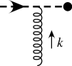
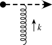
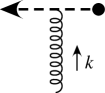
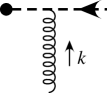
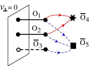
First consider the perturbative computation of attachments of usoft gluons to incoming and outgoing quark and antiquark lines. The results for the eikonal factors for one gluon are summarized in Fig. 1, and can be computed directly with the SCET collinear quark Lagrangian (or from an appropriate limit of the QCD propagator). These attachments seem to force one to make a particular choice for $s_{0}$ and $\overline{s}_{0}$, see for example the recent detailed study in Ref. Chay et al. (2005b). In our notation it is straightforward to show that this choice corresponds to

$$s_{0}=-\infty\,\textrm{sign}(\bar{\mathcal{P}})\,,\quad\overline{s}_{0}=+\infty\,\textrm{sign}(\bar{\mathcal{P}}^{\dagger})\,,\quad\left\{\begin{matrix}\tilde{\textrm{P}}\!=\!\tilde{\textrm{P}}^{\prime}\!=\!{\textrm{P}}\,,\ \ {\textrm{for}}\ \ \bar{\mathcal{P}},\bar{\mathcal{P}}^{\dagger}>0\\ \tilde{\textrm{P}}\!=\!\tilde{\textrm{P}}^{\prime}\!=\!\overline{\textrm{P}}\,,\ \ {\textrm{for}}\ \ \bar{\mathcal{P}},\bar{\mathcal{P}}^{\dagger}<0\end{matrix}\right.\,.$$ (21)

To see this take a quark with label ${\bar{n}}\!\cdot\!p>0$ and an antiquark with label ${\bar{n}}\!\cdot\!p^{\prime}<0$, and note that

$$Y\xi_{n,p} =\tilde{\textrm{P}}\exp\Big{(}ig\!\int^{0}_{-\infty}\!\!\!\!\!ds\ n\!\cdot\!A_{us}(x_{s}^{\mu})\Big{)}\xi_{n,p}^{+}={\textrm{P}}\exp\Big{(}ig\!\int^{0}_{-\infty}\!\!\!\!\!ds\ n\!\cdot\!A_{us}(x_{s}^{\mu})\Big{)}\xi_{n,p}^{+}\equiv Y_{+}\xi_{n,p}^{+}\,,$$ (22)

$$\bar{\xi}_{n,p}Y^{\dagger}\! =\bar{\xi}_{n,p}^{+}\tilde{\textrm{P}}^{\prime}\exp\Big{(}\!-\!ig\!\int^{0}_{\infty}\!\!\!\!\!ds\ n\!\cdot\!A_{us}(x_{s}^{\mu})\Big{)}\!=\bar{\xi}_{n,p}^{+}{\textrm{P}}\exp\Big{(}ig\!\int_{0}^{\infty}\!\!\!\!\!ds\ n\!\cdot\!A_{us}(x_{s}^{\mu})\Big{)}\equiv\bar{\xi}_{n,p}^{+}Y^{\dagger}_{+}\,,$$

$$Y\xi_{n,p^{\prime}}\! =\tilde{\textrm{P}}\exp\Big{(}ig\!\!\int^{0}_{\infty}\!\!\!\!ds\>n\!\cdot\!A_{us}(x_{s}^{\mu})\Big{)}\xi_{n,p^{\prime}}^{-}=\overline{\textrm{P}}\exp\Big{(}\!\!-\!\!ig\!\int_{0}^{\infty}\!\!\!\!\!ds\>n\!\cdot\!A_{us}(x_{s}^{\mu})\Big{)}\xi_{n,p^{\prime}}^{-}\equiv Y_{-}\xi_{n,p^{\prime}}^{-}\,,$$

$$\bar{\xi}_{n,p^{\prime}}Y^{\dagger}\! =\bar{\xi}_{n,p^{\prime}}^{-}\tilde{\textrm{P}}^{\prime}\exp\Big{(}\!\!-\!\!ig\!\int^{0}_{-\infty}\!\!\!\!\!\!ds\>n\!\cdot\!A_{us}(x_{s}^{\mu})\Big{)}\!=\bar{\xi}_{n,p^{\prime}}^{-}\overline{\textrm{P}}\exp\Big{(}\!\!-\!\!ig\!\int^{0}_{-\infty}\!\!\!\!\!\!ds\>n\!\cdot\!A_{us}(x_{s}^{\mu})\Big{)}\equiv\bar{\xi}_{n,p^{\prime}}^{-}Y_{-}^{\dagger}\,.$$

This is in agreement with the $\tilde{Y}=Y_{-}$, $Y^{\dagger}=Y_{-}^{\dagger}$, $Y=Y_{+}$, $\tilde{Y}^{\dagger}=Y_{+}^{\dagger}$ used in Chay et al. (2005b) for the production and annihilation of antiparticles and the annihilation and production of particles respectively. The results in Eq. (22) reproduce the natural choice of having incoming quarks/antiquarks enter from $-\infty$, while outgoing quarks/antiquarks extend out to $+\infty$.

Although the choice in Eq. (21) agrees with the $i\epsilon$’s in Fig. 1 it causes complications in the attachments of usoft gluons to internal collinear propagators. With Eq. (21) we have $s_{0}^{\dagger}\neq\overline{s}_{0}$. Now the field redefinition still induces factors of $Y^{\dagger}_{+}Y_{-}=1$ and $Y^{\dagger}_{-}Y_{+}=1$ in production and annhilation terms in the collinear Lagrangian, but it also induces factors of $Y^{\dagger}_{+}Y_{+}=Y_{\infty}$ and $Y_{-}^{\dagger}Y_{-}=Y_{\infty}^{\dagger}$ in quark-quark and antiquark-antiquark terms in the action, where

$$Y_{\infty}={\textrm{P}}\exp\Big{(}ig\!\int^{+\infty}_{-\infty}\!\!\!\!\!ds\ n\!\cdot\!A_{us}(x_{s}^{\mu})\Big{)}\,.$$ (23)

When usoft gluons attach to a collinear propagator with endpoints $x$ and $y$ we must end up with a finite Wilson line $Y(x,y)$. In the original collinear Lagrangian (prior to the field redefinition) this finite Wilson line is generated by the time ordering of fields in the usoft gluon interaction vertices. If a field redefinition is made with boundary conditions satifying $s_{0}^{\dagger}=\overline{s}_{0}$ then the vertices bordering a collinear propagator induce Wilson lines whose $s_{0}$ dependence cancels, leaving this same finite Wilson line. For example, with $s_{0}=-\infty$, $Y(-\infty,x)Y(-\infty,0)^{\dagger}=Y(0,x)$. A choice like that in Eq. (21) is more complicated since it violates hermiticity: $(\xi_{n})^{\dagger}=\xi_{n}^{\dagger}$ prior to the field redefinition, but this is no longer true for the $\xi_{n}$ and $\bar{\xi}_{n}$ fields after the field redefinition. Correspondingly, the term in the action determining the free propagator depends on $Y_{\infty}$. Thus, in this case there are $Y$ factors in both the propagators and vertices which must be taken into account in order for the path ordering not to conflict with the result from time ordering, and give the same finite Wilson line.

Let’s adopt the choice in Eq. (18) rather than Eq. (21) and check that the theory with the field redefinition in Eq. (6) still correctly reproduces the results in Fig. 1 for this case. Here we have $Y=Y_{+}$, $Y^{\dagger}=Y_{-}^{\dagger}$ for particles and antiparticles. Thus, the correct $i\epsilon$’s are obviously reproduced for the incoming collinear lines as well as intermediate propagator states. On the other hand, the result for an outgoing quark seems to have the wrong factor since $\bar{\xi}_{n}^{+}$ comes with a $Y_{-}^{\dagger}$ rather than a $Y_{+}^{\dagger}$. However, with the standard definition of an outgoing state there is actually an extra $Y_{\infty}$ induced by the field redefinition on the out-state itself. When we take this factor into account we have $Y_{\infty}Y_{-}^{\dagger}=Y_{+}^{\dagger}$ as expected. To see this, recall that an outgoing collinear quark state ${}_{\textrm{o}ut}\langle\vec{p}|$ is generated by a suitably weighted integral over $\langle 0|\xi_{n}^{+}(x_{T})$, in the large time limit $T\to\infty$ for $x_{T}=(T,\vec{x})$. When we make the field redefinition this field, $\xi_{n}^{+}(x_{T})$ generates an usoft Wilson line which extends from our reference point $s_{0}=-\infty$ to the ${\bar{n}}\!\cdot\!x$ point for our asymptotic outgoing state (which is $+\infty$ for $T\to\infty$), namely a factor of $Y_{\infty}$. A similar argument applies for outgoing antiquark states, where we get $Y_{+}Y_{\infty}^{\dagger}=Y_{-}$. The same considerations must also be made for hadronic bound states where they apply to the interpolating quark/antiquark fields used along with the LSZ formula to define the outgoing state. The factors of $Y_{\infty}$ are universal, independent of which out-state we choose. There are no additional factors for our incoming states since our reference point and $T=-\infty$ coincide, $Y(-\infty,-\infty)=1$. Once the $Y_{\infty}$ factors are taken into account, the choice in Eq. (18) correctly reproduces the path for outgoing quark and antiquark lines. If we had instead made the choice for $s_{0}$ in Eq. (19) (which also satisfies $s_{0}^{\dagger}=\overline{s}_{0}$) then we would have $Y_{\infty}^{(\dagger)}$ factors for incoming antiquark states and outgoing quark states, but the final outcome is the same. Thus the complete result is independent of the $s_{0}$ choice.

The above discussion covers usoft interactions from the collinear Lagrangian, but it is also worth remarking on the interactions induced by the field redefinition in (possibly non-local) operators that are not time ordered. We continue to use Eq. (18). Here again, the identity $Y^{\dagger}Y=1$ is important in order to prove the cancellation of usoft gluon attachments. It is convenient to adopt a convention where one collects the extra factors of $Y_{\infty}$ induced from outgoing states together with the $Y^{\dagger}$’s from production fields in these operators. In this case if we consider $J(x)=\bar{\xi}_{n}^{+}\,\bar{n}\!\!\!/\,\xi_{n}^{-}$ for the production of a collinear quark and antiquark, then instead of writing only the $Y_{-}^{\dagger}$ and $Y_{+}$ from the fields we write $J\to\bar{\xi}_{n}^{+}Y_{+}^{\dagger}\,\bar{n}\!\!\!/\,Y_{-}\,\xi_{n}^{-}$ = $\bar{\xi}_{n}^{+}\,\bar{n}\!\!\!/\,\xi_{n}^{-}$ which includes the $Y$’s from any out-state this current could produce. Here the usoft interactions in the $Y$ and $Y^{\dagger}$ lines extend from $x$ to $\infty$ and cancel. For the annihilation of a quark and antiquark the lines extend from $-\infty$ to $x$ and also cancel, namely $Y^{\dagger}_{-}Y_{+}=1$. These two cancellations are often sufficient to ensure the decoupling of usoft gluons. For example, in exclusive processes we must have color singlet combinations to connect to incoming or outgoing collinear hadrons and so we can typically pair up $\bar{\xi}_{n}^{\pm}$ and $\xi_{n}^{\mp}$ fields in the hard scattering operator and make the cancellations manifest.

If we instead consider an inclusive process like DIS then we have a quark scattered to a quark (we consider generic Bjorken $x<1$ in the Breit frame). In this case including the $Y_{\infty}$ from one outgoing quark in the final state gives $\bar{\xi}_{n}^{+}\,\bar{n}\!\!\!/\,\xi_{n}^{+}\to\bar{\xi}_{n}^{+}Y_{+}^{\dagger}\,\bar{n}\!\!\!/\,Y_{+}\xi_{n}^{+}$ where the Wilson lines do not seem to cancel. Here in order for the cancellation of usoft gluons to take place it is important to either a) take into account all factors of $Y_{\infty}$ from the outgoing proton state, or b) include the $Y_{\infty}$ from one outgoing quark state but note that we are only matching cut diagrams for this inclusive process. The choice a) or b) depends on whether we want to take the imaginary part at the very end, or from the beginning. For b) the effective theory computation has the imaginary part of the hard computation, but the imaginary part also effects the collinear operator, where we can denote the cut by a vertical line, $\big{|}$. With our initial state for the $T$-matrix taken on the RHS of the cut, the signs are as in Fig. 1, but on the LHS we have the complex conjugate of these expressions, and the above computation becomes

$$(\bar{\xi}_{n})\big{|}(\bar{n}\!\!\!/\xi_{n})\to(\bar{\xi}_{n}Y_{-}^{\dagger})\big{|}(\bar{n}\!\!\!/Y_{+}\xi_{n})=\bar{\xi}_{n}\,\bar{n}\!\!\!/\,\xi_{n}\,.$$ (24)

Thus, the usoft gluon interactions also cancel in this case. Alternatively, with a) one must keep track of all the lines in the full forward scattering calculation including $Y_{\infty}^{(\dagger)}$ factors from all initial and/or final state quarks, and then the $Y$’s in the low energy theory again all cancel. Both ways we arrive at the same final result, $({\textrm{Im}}\,C)\bar{\xi}_{n}\bar{n}\!\!\!/\xi_{n}$ (see Refs. Bauer et al. (2002b); Manohar (2003) for a discussion of DIS in SCET). Similar considerations can be applied to $B\to X_{s}\gamma$ in the endpoint region. The $s_{0}$ dependence cancels, and for this process we are left with a finite usoft Wilson line, $\bar{h}_{v}(x)Y(x,0)h_{v}(0)$.

To summarize, keeping careful track of the boundary condition $s_{0}$ dependence in the usoft Wilson line $Y$, a choice satisfying $s_{0}=\overline{s}_{0}^{\dagger}$ appears to be the most natural (even though there will be additional $Y_{\infty}$ factors from states). Physical results are independent of the choice made for the $s_{0}$ reference point. They may still depend on the path of Wilson lines in the final result, but this is determined by the universal class of processes described by the operator rather than the choice of $s_{0}$ in the field redefinition. Similar conclusions hold for the path dependence in collinear Wilson lines $W$. We note that with respect to the definitions of the gauge invariant structures made in Eq.(II.1), the remaining allowed global color rotations simply correspond to color rotations at the reference point. We will pick the same reference point in $W$ and $Y$ factors. For example, the gauge invariant product of fields $(Y^{\dagger}h_{v})$ carries a color index in the 3 representation, which by convention is acted on by global rotations $U(s_{0})$, via $(Y^{\dagger}h_{v})\to U(s_{0})(Y^{\dagger}h_{v})$. These color rotations still connect invariant products of collinear and usoft fields.

II.3 Reparameterization invariance

The structure of the currents is constrained by reparameterization invariance, which is an invariance that appears due to the ambiguity in the decomposition of momenta in terms of basis vectors and in terms of large and small components. The total momentum $P^{\mu}$ of a heavy quark is decomposed as

$$P^{\mu}=m_{Q}v^{\mu}+k^{\mu},$$

where $m_{Q}$ is the quark’s mass, $v^{\mu}$ is its velocity, and $k^{\mu}$ is a residual momentum of order $m_{Q}\lambda^{2}$. Then the simultaneous shifts

$$v^{\mu}\rightarrow v^{\mu}+\beta^{\mu}\quad\text{and}\quad k^{\mu}\rightarrow k^{\mu}-m_{Q}\beta^{\mu},$$ (25)

where the infinitesimal $\beta^{\mu}\sim\lambda^{2}$, can have no physical consequences Luke and Manohar (1992). We refer below to this reparameterization invariance as HQET-RPI. The transformation of the field ${\mathcal{H}}_{v}\to{\mathcal{H}}_{v}+\delta{\mathcal{H}}_{v}$ induces terms at ${\mathcal{O}}(\lambda^{0})$ and ${\mathcal{O}}(\lambda^{2})$,

$$\delta^{(\lambda^{0})}{\mathcal{H}}_{v}=(im\beta\cdot x){\mathcal{H}}_{v}\,,\qquad\quad\delta^{(\lambda^{2})}{\mathcal{H}}_{v}=\frac{\beta\!\!\!/}{2}\>{\mathcal{H}}_{v}.$$ (26)

There are also reparameterization invariances associated with ambiguities in the decomposition of the momenta of collinear fields. Here the total momentum $P^{\mu}$ of a collinear particle is decomposed into the sum of a collinear momentum $p^{\mu}$, with $(n\cdot p,\bar{n}\cdot p,p_{\bot})\sim Q(\lambda^{2},1,\lambda)$, and an ultrasoft momentum $k^{\mu}$, with $(n\cdot k,\bar{n}\cdot k,k_{\bot})\sim Q(\lambda^{2},\lambda^{2},\lambda^{2})$:

$$P^{\mu} = p^{\mu}+k^{\mu}$$ (27)

$$= \frac{n^{\mu}}{2}\bar{n}\cdot(p+k)+\frac{\bar{n}^{\mu}}{2}n\cdot k+(p_{\bot}+k_{\bot}).$$ (28)

This decomposition has two types of ambiguity. The first comes from splitting $P^{\mu}$ into large ($p$) and small ($k$) components. Thus operators must be invariant under a transformation that takes

$$\overline{\mathcal{P}}\rightarrow\overline{\mathcal{P}}+\bar{n}\cdot\ell\,,\qquad\quad i\bar{n}\cdot\partial\rightarrow i\bar{n}\cdot\partial-\bar{n}\cdot\ell\,,$$

$${\mathcal{P}}_{\perp}^{\mu}\rightarrow{\mathcal{P}}_{\perp}^{\mu}+\ell_{\perp}^{\mu}\,,\qquad\quad i\partial_{\perp}^{\mu}\rightarrow i\partial_{\perp}^{\mu}-\ell_{\perp}^{\mu},$$ (29)

where all operators and derivatives act on one or more collinear fields, and $\ell^{\mu}$ is ${\mathcal{O}}(\lambda^{2})$. We refer to this reparameterization invariance as SCET RPI-a. Examples of an infinitesimal transformation on fields and operators are

$$\delta_{a}^{(\lambda^{0})}\chi_{n}=(i\ell\cdot x)\chi_{n}\,,\qquad\delta_{a}^{(\lambda^{1})}{\mathcal{P}}_{\perp}^{\alpha}=\ell^{\alpha}_{\perp}\,,\qquad\delta_{a}^{(\lambda^{2})}\bar{\mathcal{P}}={\bar{n}}\!\cdot\!\ell\,,$$ (30)

where $n\!\cdot\!\ell=0$. Note that $(i\ell\cdot x)$ terms only effect ultrasoft derivatives acting on the fields since the overall current is evaluated at $x=0$.

The second ambiguity in the decomposition of the momentum of the collinear particles comes from choosing the light-cone vectors $n$ and $\bar{n}$. An infinitesimal change in these vectors which preserves the relations $n^{2}=0$, $\bar{n}^{2}=0$, and $n\cdot\bar{n}=2$, can have no physical consequences. The most general infinitesimal transformations of $n$ and $\bar{n}$ that preserve these conditions along with the collinear power counting are Manohar et al. (2002)

$$\text{(I)}\left\{\begin{tabular}[]{l}$n_{\mu}\to n_{\mu}+\Delta_{\mu}^{\perp}$\\ $\bar{n}_{\mu}\to\bar{n}_{\mu}$\end{tabular}\right.\qquad\text{(II)}\left\{\begin{tabular}[]{l}$n_{\mu}\to n_{\mu}$\\ $\bar{n}_{\mu}\to\bar{n}_{\mu}+\varepsilon_{\mu}^{\perp}$\end{tabular}\right.\qquad\text{(III)}\left\{\begin{tabular}[]{l}$n_{\mu}\to(1+\alpha)\,n_{\mu}$\\ $\bar{n}_{\mu}\to(1-\alpha)\,\bar{n}_{\mu}$\end{tabular}\right.\,,$$ (37)

where $\{\Delta^{\bot}_{\mu},\epsilon^{\bot}_{\mu},\alpha\}\sim\{\lambda^{1},\lambda^{0},\lambda^{0}\}$ are five infinitesimal parameters, and $\bar{n}\cdot\epsilon^{\bot}=n\cdot\epsilon^{\bot}=\bar{n}\cdot\Delta^{\bot}=n\cdot\Delta^{\bot}=0$.

If we start in the frame $v_{\bot}=0$, then transformations (I) or (II) or (HQET-RPI) take us out of this frame. A certain combined type I and type II transformation, however, leaves $v_{\perp}=0$ Hill et al. (2004). We refer to this transformation as RPI-$\star$. We can also form a combined HQET and type II transformation that leaves $v_{\perp}=0$ which we refer to as RPI-$\$$. These transformations are

$$(\star)\left\{\begin{tabular}[]{l}$n_{\mu}\to n_{\mu}+\Delta_{\mu}^{\perp}$\\ $\bar{n}_{\mu}\to\bar{n}_{\mu}-\frac{\Delta^{\bot}_{\mu}}{(n\cdot v)^{2}}$\\ $v_{\mu}\to v_{\mu}$\end{tabular}\right.\,,\qquad\qquad\quad(\$)\left\{\begin{tabular}[]{l}$v^{\mu}\to v^{\mu}+\beta_{T}^{\mu}$\\ $\bar{n}^{\mu}\to\bar{n}^{\mu}+\frac{2}{n\cdot v}\>\beta_{\perp}^{\mu}$\\ $n_{\mu}\to n_{\mu}$\end{tabular}\right.\,,$$ (44)

where $\Delta^{\bot}\sim\lambda$, $\beta\sim\lambda^{2}$, and $\beta_{\perp}$ is the $\perp$-part of $\beta_{T}$. In defining the $-transformation we found that it is more convenient to leave $v_{\perp}=0$ by making a transformation on $v$ simultaneously with ${\bar{n}}$, rather than simultaneously with $n$. Under the $\star$-transformation the components of a generic four-vector $V_{\mu}$ transform as

$$n\cdot V \stackrel{{\scriptstyle\star}}{{\longrightarrow}}n\cdot V+\Delta^{\perp}\cdot V^{\perp}\,,$$

$${\bar{n}}\cdot V \stackrel{{\scriptstyle\star}}{{\longrightarrow}}{\bar{n}}\cdot V-\frac{\Delta^{\perp}\cdot V^{\perp}}{(n\!\cdot\!v)^{2}}\,,$$

$$V^{\perp}_{\mu} \stackrel{{\scriptstyle\star}}{{\longrightarrow}}V^{\perp}_{\mu}+\Delta^{\perp}_{\mu}\Big{(}-\frac{{\bar{n}}}{2}+\frac{n}{2(n\!\cdot\!v)^{2}}\Big{)}\cdot V+\Big{(}-\frac{{\bar{n}}_{\mu}}{2}+\frac{n_{\mu}}{2(n\!\cdot\!v)^{2}}\Big{)}\Delta^{\perp}\cdot V^{\perp}\,.$$ (45)

To the order we are working we need the following terms from an RPI-$\star$ transformation:

$$\delta_{\star}^{(\lambda^{0})}{\mathcal{P}}_{\perp}^{\mu} = -\frac{\Delta_{\perp}^{\mu}}{2}\>\bar{\mathcal{P}}\,,\qquad\qquad\qquad\ \ \>\delta_{\star}^{(\lambda^{0})}(ign\!\cdot\!{\mathcal{B}})=\Delta_{\perp}\cdot(ig{\mathcal{B}_{\perp}})\,,$$ (46)

$$\delta_{\star}^{(\lambda^{0})}(ig{\mathcal{B}_{\perp}^{\mu}}) = 0\,,\qquad\qquad\qquad\qquad\qquad\quad\ \ \,\delta_{\star}^{(\lambda^{0})}\bar{\chi}_{n}=0\,,$$

$$\delta_{\star}^{(\lambda^{1})}{\mathcal{P}}_{\perp}^{\mu} = ({\bar{n}}\!\cdot\!v)^{2}n_{T}^{\mu}\>\Delta^{\perp}\!\cdot\!{\mathcal{P}}_{\perp}\,,\qquad\qquad\quad\delta_{\star}^{(\lambda^{1})}\bar{\chi}_{n}=\bar{\chi}_{n}\>\frac{\bar{n}\!\!\!/\Delta\!\!\!\!/^{\perp}}{4}\,,$$

$$\delta_{\star}^{(\lambda^{1})}(ig{\mathcal{B}^{\mu}_{\perp}}) = ({\bar{n}}\!\cdot\!v)^{2}n_{T}^{\mu}\>\Delta^{\perp}\!\cdot\!(ig{\mathcal{B}}_{\perp})\,,\qquad\qquad\!\!\delta_{\star}^{(\lambda^{2})}\bar{\mathcal{P}}=-({\bar{n}}\!\cdot\!v)^{2}\Delta_{\perp}\cdot{\mathcal{P}}_{\perp}\,,$$

$$\delta_{\star}^{(\lambda^{2})}\bar{\chi}_{n} = -\bar{\chi}_{n}\Big{(}ig{\mathcal{B}}\!\!\!/^{\perp}+{\mathcal{P}}\!\!\!\!/^{\perp\,\dagger}\Big{)}\frac{1}{{\bar{\mathcal{P}}}^{\dagger}}\frac{\Delta\!\!\!\!/^{\perp}}{2(n\!\cdot\!v)^{2}}+\bar{\chi}_{n}\Big{[}\frac{1}{(n\!\cdot\!v)^{2}\bar{{\mathcal{P}}}}\>ig{\mathcal{B}}^{\perp}\!\cdot\!\Delta^{\perp}\Big{]}\,,$$

where $n_{T}$ is the transverse part of $n$,

$$n_{T}^{\mu}=n^{\mu}-n\!\cdot\!v\,v^{\mu}=\frac{n^{\mu}}{2}-{(n\!\cdot\!v)}^{2}\frac{\bar{n}^{\mu}}{2}\,.$$ (47)

We will also need the transformation

$$\delta_{\star}^{(\lambda^{2})}\delta(\omega-n\!\cdot\!v\bar{\mathcal{P}}^{\dagger}) = \frac{1}{n\!\cdot\!v}\>\Delta_{\perp}\!\cdot\!{\mathcal{P}}_{\perp}^{\dagger}\>\delta^{\prime}(\omega-n\!\cdot\!v\bar{\mathcal{P}}^{\dagger})\,.$$ (48)

For the RPI-$\$$ transformation at the order we are working we need the following terms:

$$\delta_{\$}^{(\lambda^{0})}{\mathcal{H}}_{v} =(im\beta_{T}\cdot x){\mathcal{H}}_{v}\,, \delta_{\$}^{(\lambda^{2})}{\mathcal{H}}_{v} =\frac{\beta\!\!\!/_{T}}{2}\ {\mathcal{H}}_{v}\,,$$ (49)

$$\delta_{\$}^{(\lambda^{2})}\>\delta(\omega-n\!\cdot\!v\bar{\mathcal{P}}^{\dagger}) =-n\!\cdot\!\beta_{T}\>\bar{\mathcal{P}}^{\dagger}\>\delta^{\prime}(\omega-n\!\cdot\!v\bar{\mathcal{P}}^{\dagger})\,.$$

For the last identity it is straightforward to see that the $-transformation on ${\bar{n}}$ does not enter until one higher order. We chose to define the RPI-$\$$ transformation to be for $v$ and ${\bar{n}}$ rather than $v$ and $n$ because of the property that terms with ${\bar{n}}$ are often pushed to higher order, making the relations derived with RPI-$\$$ more orthogonal to those from RPI-$\star$. For example, in order to have a simple form for the $\delta_{\$}\Gamma$’s in Eq. (82) below it is important that it is ${\bar{n}}$ and not $n$ that transforms. Finally, we note that since all Dirac structures are $\mathcal{O}(1)$, all RPI transformations of Dirac structures have the same power counting as the transformation parameter, in particular, $\delta_{\star}\Gamma\sim\mathcal{O}(\lambda^{1})$ and $\delta_{\$}\Gamma\sim\mathcal{O}(\lambda^{2})$.

Finally, note that we will consider the RPI tranformations of all currents prior to making the field redefinition in Eq. (6) so that we do not have to transform $Y$. However, in order not to have to switch our notation back and forth we will write all equations with the operators obtained after the field redefinition. This implies that results quoted for the transformation of objects involving ${\cal H}_{v}$ should be though of as being made for $h_{v}$, with the field redefinition which induces ${\cal H}_{v}$ made only afterwards.

II.4 Completeness of Projected RPI

It is natural to ask if for $v_{\perp}=0$ the transformations RPI-$\$$ and RPI-$\star$ in Eq. (44) are sufficient to give the complete set of constraints that arise from the original SCET type-I, SCET type-II, and HQET RPI transformations. The set $\{$ RPI-$\$$, RPI-$\star$, SCET-II $\}$ forms an equivalent complete grouping related by linear combinations. To address this question, consider splitting all possible operators into two sets, a set $\{{\mathrm{O}}_{i}\}$ which do not vanish on the $v_{\perp}=0$ surface and a set $\{\overline{\mathrm{O}}_{i}\}$ which do. An example is pictured in Fig. 2.

Figure 2: Transformation of operators on and off the $v_{\perp}=0$ surface. Here ${\mathrm{O}}_{1,2}$ exist for $v_{\perp}=0$, while $\overline{\mathrm{O}}_{3,4,5}$ vanish on the $v_{\perp}=0$ surface.

Constraints are derived by requiring cancellations among the resulting post-transformation set of operators. If we consider an operator $\mathrm{O}_{i}$ then under one of the projected RPI transformations, RPI-$\$$ or RPI-$\star$, it transforms into the set $\{\mathrm{O}_{j},\overline{\mathrm{O}}_{k}\}$. On the other hand an operator $\overline{\mathrm{O}}_{i}$ only transforms back into the set $\{\overline{\mathrm{O}}_{j}\}$. This is a special feature of the projected transformations and ensures that relations derived on the $v_{\perp}=0$ surface can not be spoiled by operators which appear away from the surface. It appears that we can neglect the $\overline{\mathrm{O}}_{i}$ operators since they vanish when we project on the $v_{\perp}=0$ plane. However it is still possible that we will miss an additional relation between operators on the surface, so that the surface analysis will not be complete.

There are two possible sources that could lead to additional relations beyond those derived from projected RPI on the surface. First, under the SCET RPI-II transformation $\epsilon_{\perp}\sim\lambda^{0}$ is allowed, while in the RPI-$\star$ and RPI-$\$$ transformations we only have smaller transformations of ${\bar{n}}$ of ${\cal O}(\lambda^{1})$ and ${\cal O}(\lambda^{2})$. Thus we could miss relations from the more restrictive $\epsilon_{\perp}\sim\lambda^{0}$ allowed by SCET RPI-II. Note that an SCET RPI-II transformation takes us off the projected surface. Second if we project onto $v_{\perp}=0$ then constraints are derived only by enforcing cancellations within the set $\{\mathrm{O}_{j}\}$. It is possible that an operator ${\overline{\mathrm{O}}}_{4}$ exists that is obtained from the transformation of two operators $O_{1}$ and $O_{2}$ that are not related by transformations on the surface. Enforcing the cancellation of ${\overline{\mathrm{O}}}_{4}$ then relates ${\mathrm{O}_{1}}$ and ${\mathrm{O}_{2}}$. This is pictured by the star in Fig. 2. A related alternative is an operator like ${\overline{\mathrm{O}}}_{5}$ pictured with the box which is obtained from transformations of ${\mathrm{O}_{1,2}}$ and $\overline{\mathrm{O}_{3}}$. If $\overline{\mathrm{O}_{3}}$ is otherwise constrained then this would also constrain ${\mathrm{O}_{1,2}}$. In cases with multiple operators appearing and multiple transformations we must of course consider the linear independence of combinations of operators. If an $\overline{\mathrm{O}}_{i}$ contributes and it is not otherwise constrained then this is not of concern, since in the end we discard ${\overline{\mathrm{O}}}_{i}$ by projecting onto the $v_{\perp}=0$ surface anyway. We will call an operator that vanishes for $v_{\perp}=0$ but that generates a relation between operators on the surface a “supplementary projected operator” (SPO). To check for the existence of an SPO we might in general need the full set of $v_{\perp}\neq 0$ operators. At ${\cal O}(\lambda)$ the comparison of the results derived in Ref. Pirjol and Stewart (2003) in the full space, to those derived in Ref. Hill et al. (2004) on the surface $v_{\perp}=0$ shows that there are no SPO’s at this order.

For the ${\cal O}(\lambda^{2})$ heavy-to-light operators considered here we show that there also no SPO’s in section III.4. This is done by a careful choice of our Dirac basis which makes it simpler to demonstrate that there are no further type-II RPI relations, and by explicit construction for other possible SPO’s. Thus, the analysis on the $v_{\perp}=0$ surface is complete for our computation.

III Heavy-to-Light currents to ${\mathcal{O}}(\lambda^{2})$

To order $\lambda^{2}$, the operators and Wilson coefficients for the heavy-to-light currents can be written as

$$J= J^{(0)}+J^{(1)}+J^{(2)}$$ (50)

$$= \sum_{j}\int\!\!d\omega\,C_{j}(\omega,m,\mu)J_{j}^{(0)}(\omega,\mu)+\sum_{x,j}\int\![d\omega_{i}]\,B_{xj}(\omega_{i},m,\mu)J_{j}^{(1x)}(\omega_{i},\mu)$$

$$+\sum_{x,j}\int\![d\omega_{i}]\,A_{xj}(\omega_{i},m,\mu)J_{j}^{(2x)}(\omega_{i},\mu),$$

where $J^{(kx)}(\omega_{i})$ represents the $\mathcal{O}(\lambda^{k})$ terms with dependence on convolution parameters $\omega_{i}$. Here the subscript $x$ distinguishes distinct field structures at a given order, and $j$ sums over distinct Dirac structures. At ${\mathcal{O}}(\lambda)$ we know that there are at most two relevant convolution parameters $i=1,2$, while we will see below that at ${\mathcal{O}}(\lambda^{2})$ there are at most three. We will consider both scalar, vector, and tensor currents (and the simple extension to the pseudoscalar and axial vector cases). When necessary we add an $(s)$, $(v)$, or $(t)$ superscript to the Wilson coefficients in order to distinguish these cases, e.g. $B_{a1}^{(v)}$.

We begin in section III.1 by constructing all consistent field structures for the NNLO currents. In section III.2 we use reparameterization invariance to derive the constraint equations for these currents under different types of RPI invariance on the $v_{\perp}=0$ surface. In section III.3 we solve the constraint equations to find the allowed Dirac structures and obtain relations among the Wilson coefficients. Finally, in section III.4 we show that the results from the $v_{\perp}=0$ surface are equivalent to those obtained if all relations in the full space were projected onto this plane.

III.1 Current field structures at ${\mathcal{O}}(\lambda^{2})$

We first construct a basis of currents that is consistent with gauge invariance and power counting and eliminate structures that are redundant by the equations of motion and Bianchi identity. At LO and NLO the currents are

$$J^{(0)}(\omega) = \bar{\chi}_{n,\omega}\Gamma{\mathcal{H}}_{v}\,,$$ (51)

$$J^{(1a)}(\omega) = \frac{1}{\omega}\>\bar{\chi}_{n,\omega}\mathcal{P}^{\bot\dagger}_{\alpha}\Theta^{\alpha}_{(a)}{\mathcal{H}}_{v}$$

$$J^{(1b)}(\omega_{1,2}) = \frac{1}{m}\>\bar{\chi}_{n,\omega_{1}}(ig\mathcal{B}^{\bot}_{\alpha})_{\omega_{2}}\Theta^{\alpha}_{(b)}{\mathcal{H}}_{v}\,.$$

At NNLO we find that a convenient basis for the set of field structures for the bilinear quark operators is

$$J^{(2a)}(\omega) =\frac{1}{2m}\>\bar{\chi}_{n,\omega}\Upsilon^{\sigma}_{(a)}i{\mathcal{D}}^{T}_{us\,\,\sigma}{\mathcal{H}}_{v}\,,$$ (52)

$$J^{(2b)}(\omega) =-\frac{n\!\cdot\!v}{\omega}\>\bar{\chi}_{n,\omega}\,i\bar{n}\cdot\overleftarrow{{\mathcal{D}}}_{us}\Upsilon_{(b)}{\mathcal{H}}_{v}\,,$$

$$J^{(2c)}(\omega) =-\frac{1}{\omega}\>\bar{\chi}_{n,\omega}i\overleftarrow{{\mathcal{D}}}_{us\,\alpha}^{\bot}\,\Upsilon^{\alpha}_{(c)}{\mathcal{H}}_{v}\,,$$

$$J^{(2d)}(\omega) =\frac{1}{\omega^{2}}\>\bar{\chi}_{n,\omega}\mathcal{P}^{\bot\dagger}_{\alpha}\mathcal{P}^{\bot\dagger}_{\beta}\Upsilon_{(d)}^{\alpha\beta}{\mathcal{H}}_{v}\,,$$

$$J^{(2e)}(\omega_{1,2}) =\frac{1}{m(\omega_{1}+\omega_{2})}\>\bar{\chi}_{n,\omega_{1}}(ig\mathcal{B}^{\bot}_{\alpha})_{\omega_{2}}\mathcal{P}^{\bot\dagger}_{\beta}\Upsilon_{(e)}^{\alpha\beta}{\mathcal{H}}_{v}\,,$$

$$J^{(2f)}(\omega_{1,2}) =\frac{\omega_{2}}{m(\omega_{1}+\omega_{2})}\>\bar{\chi}_{n,\omega_{1}}\bigg{(}\frac{\mathcal{P}^{\bot}_{\beta}}{\omega_{2}}+\frac{\mathcal{P}^{\bot\dagger}_{\beta}}{\omega_{1}}\bigg{)}(ig\mathcal{B}^{\bot}_{\alpha})_{\omega_{2}}\Upsilon_{(f)}^{\alpha\beta}{\mathcal{H}}_{v}\,,$$

$$J^{(2g)}(\omega_{1,2}) =\frac{1}{m\,n\!\cdot\!v}\>\bar{\chi}_{n,\omega_{1}}\Big{\{}(ign\cdot\mathcal{B})_{\omega_{2}}+2(ig{\mathcal{B}_{\perp}})_{\omega_{2}}\cdot{\mathcal{P}}_{\perp}^{\dagger}\frac{1}{\bar{\mathcal{P}}^{\dagger}}\Big{\}}\Upsilon_{(g)}{\mathcal{H}}_{v}\,,$$

$$J^{(2h)}(\omega_{1,2,3}) =\frac{1}{m(\omega_{2}+\omega_{3})}\>\bar{\chi}_{n,\omega_{1}}(ig\mathcal{B}^{\bot}_{\beta})_{\omega_{2}}(ig\mathcal{B}^{\bot}_{\alpha})_{\omega_{3}}\Upsilon_{(h)}^{\alpha\beta}{\mathcal{H}}_{v}\,,$$

$$J^{(2i)}(\omega_{1,2,3}) =\frac{1}{m(\omega_{2}+\omega_{3})}\mathrm{Tr}[(ig\mathcal{B}^{\bot}_{\beta})_{\omega_{2}}(ig\mathcal{B}^{\bot}_{\alpha})_{\omega_{3}}]\>\bar{\chi}_{n,\omega_{1}}\Upsilon_{(i)}^{\alpha\beta}{\mathcal{H}}_{v}\,.$$

For a basis of four quark operators we take

$$J^{(2j)}(\omega_{1},\omega_{2},\omega_{3}) =\sum_{f=u,d,s}\bigl{[}\bar{\chi}^{f}_{n,\omega_{2}}\Upsilon_{(j\chi)}\chi_{n,\omega_{3}}^{f}\bigr{]}\bigl{[}\bar{\chi}_{n,\omega_{1}}\Upsilon_{(j\mathcal{H})}{\mathcal{H}}_{v}\bigr{]}\,,$$

$$J^{(2k)}(\omega_{1},\omega_{2},\omega_{3}) =\sum_{f=u,d,s}\bigl{[}\bar{\chi}^{f}_{n,\omega_{2}}T^{A}\Upsilon_{(k\chi)}\chi_{n,\omega_{3}}^{f}\bigr{]}\bigl{[}\bar{\chi}_{n,\omega_{1}}T^{A}\Upsilon_{(k\mathcal{H})}{\mathcal{H}}_{v}\bigr{]}$$ (53)

where the matrices $T^{A}$ are generators of SU(3) with an implied sum on $A$ and $\chi^{f}_{n}$ has a collinear quark with flavor $f$, whereas $\chi_{n}$ carries the flavor of quark from the full theory current. We impose the RPI type-III invariance in Eq. (37) on all operators by multiplying by an appropriate power of $n\!\cdot\!v$. The basis in Eqs. (51,52,III.1) is valid whether or not we take $v_{\perp}=0$. The $v_{\perp}=0$ choice only effects the basis of Dirac structures.

The 11 operators in Eqs. (52,III.1) can be compared with the 15 field structures in the basis of Ref. Beneke et al. (2005). We have no analog of their $J^{(2)}_{1,2,3,7}$ currents which have an explicit $x^{\mu}$ because with momentum labels the multipole expansion is performed directly in momentum space Luke et al. (2000). Correspondingly, our $J^{(2b)}$ and $J^{(2c)}$ currents have no analogs in their basis. There is a correspondence, $J^{(2a,2d)}\leftrightarrow J^{(2)}_{4,6}$, $\ J^{(2e,2f,2g)}\leftrightarrow J^{(2)}_{8,9,10}$, $\ J^{(2i,2j,2k)}\leftrightarrow J^{(2)}_{13,14,15}$, and our $J^{(2h)}$ encodes their $J^{(2)}_{12}$ and $J^{(2)}_{13}$ currents.

In arriving at Eq. (52) we have used Eq. (II.1) to switch to a basis with ${\mathcal{P}}_{\perp}$’s, $in\!\cdot\!\partial$, and field strengths rather than collinear covariant derivatives in order to give simpler constraints from RPI. The basis with covariant derivatives is more natural from the point of view of tree level matching and the relation between the two is discussed in section IV. The prefactors in $J^{(2a-2i)}$ have been chosen with these relationships in mind, in order to make the matching coefficients for the operators simple. The combinations in $J^{(2f,2g)}$ were chosen because they have simpler transformations under RPI.

Structures were also removed from Eq. (52) using equations of motion and the Bianchi identity. In the effective field theory this gives a valid basis at any loop order. After decoupling the usoft gluons the LO Lagrangian for collinear quarks is Bauer et al. (2002a)

$${\mathcal{L}}_{c}^{(0)} = \overline{\xi}_{n}\frac{\bar{n}\!\!\!/}{2}\Big{(}in\!\cdot\!D_{c}+i{/\!\!\!\!D}_{c}^{\perp}W\frac{1}{\bar{\mathcal{P}}}W^{\dagger}i{/\!\!\!\!D}_{c}^{\perp}\Big{)}\xi_{n}=\overline{\chi}_{n}\frac{\bar{n}\!\!\!/}{2}\Big{(}in\!\cdot\!{\mathcal{D}}_{c}+i{/\!\!\!\!\mathcal{D}}_{c}^{\perp}\frac{1}{\bar{\mathcal{P}}}i{/\!\!\!\!\mathcal{D}}_{c}^{\perp}\Big{)}\chi_{n}\,,$$ (54)

so the equation of motion for $\chi_{n}$ can be written

$$in\!\cdot\!\partial\chi_{n}=-(ign\!\cdot\!{\mathcal{B}})\chi_{n}-i\,{/\!\!\!\!\mathcal{D}}_{c}^{\perp}\frac{1}{\bar{\mathcal{P}}}i\,{/\!\!\!\!\mathcal{D}}_{c}^{\perp}\>\chi_{n}\,,$$ (55)

where using Eq. (II.1) the last term can be written as a sum of terms with either two ${\mathcal{P}}_{\perp}$’s, two $(ig{\mathcal{B}}_{\perp})$’s, or one of each. Eq. (55) shows that a a current $\bar{\chi}_{n}in\!\cdot\!\overleftarrow{\partial}{\mathcal{H}}^{\dagger}_{v}$ is redundant by the collinear quark equation of motion and need not be included in the list, explaining why we only have $J^{(2b)}$ and $J^{(2c)}$. (Note that $in\!\cdot\!{\mathcal{D}}_{us}\chi_{n}=in\!\cdot\!\partial\chi_{n}$.) As noted in Beneke et al. (2005), this makes their $J_{5}^{(2)}$ current redundant. In $J^{(2a)}$ we have restricted the ultrasoft derivative acting on $h_{v}$ to be purely transverse since the heavy quark equation of motion is $v\cdot D_{us}\,h_{v}\mspace{-5.0mu}=\mspace{-3.0mu}0$.

One can also consider using the collinear gluon equation of motion. After the field redefinition in Eq. (6), the lowest order collinear gluon Lagrangian is the same as in QCD Bauer et al. (2002a), ${\mathcal{L}}_{g}^{(0)}=1/(2g^{2}){\textrm{ tr}}\{[iD_{c}^{\mu},iD_{c}^{\nu}]\}^{2}$. Varying ${\mathcal{L}}_{c}^{(0)}+{\mathcal{L}}_{g}^{(0)}$ with respect to the collinear gluon field $A_{c\,\mu}^{A}$ and contracting with $\bar{n}_{\mu}T^{A}$ gives

$$0=\bar{n}_{\mu}T^{A}\frac{\delta\mathcal{L}^{(0)}}{\delta A_{c\,\mu}^{A}}=\frac{1}{g}\bar{n}_{\mu}\left[iD_{c\nu},\left[iD^{\mu}_{c},iD^{\nu}_{c}\right]\right]+gT^{A}\sum_{f}\overline{\xi}_{n}^{f}T^{A}\not{\bar{n}}\,\xi_{n}^{f}\,.$$ (56)

Next we multiply by $W^{\dagger}$ on the left and $W$ on the right, use the identity $(W^{\dagger}T^{A}W)\otimes T^{A}=T^{A}\otimes(WT^{A}W^{\dagger})$, and label by $\omega_{2}$ to give

$$-g^{2}T^{A}\sum_{f}\big{[}{\bar{\chi}}_{n}^{f}\>T^{A}\not{\bar{n}}\chi_{n}^{f}\big{]}_{\omega_{2}} =\big{(}\left[i{\mathcal{D}}_{c\nu},\left[i{\bar{n}}\!\cdot\!{\mathcal{D}}_{c},i{\mathcal{D}}^{\nu}_{c}\right]\right]\big{)}_{\omega_{2}}$$ (57)

$$=\frac{\omega_{2}^{2}}{2}(ign\!\cdot\!{\mathcal{B}})_{\omega_{2}}-\omega_{2}{\mathcal{P}}^{\perp}_{\nu}(ig{\mathcal{B}}_{\perp}^{\nu})_{\omega_{2}}-\sum_{\omega_{3}}\omega_{3}\big{[}(ig{\mathcal{B}}_{\perp}^{\nu})_{\omega_{2}-\omega_{3}},(ig{\mathcal{B}}^{\perp}_{\nu})_{\omega_{3}}\big{]}\,.$$

Multiplying by $\bar{\chi}_{n,\omega_{1}}$ on the left and $\Gamma{\mathcal{H}}_{v}$ on the right where $\Gamma$ is some Dirac structure gives

$$\frac{\omega_{2}^{2}}{2}\>\bar{\chi}_{n,\omega_{1}}(ign\!\cdot\!{\mathcal{B}})_{\omega_{2}}\Gamma{\mathcal{H}}_{v}=-g^{2}\sum_{f,\omega_{3}}\big{[}{\bar{\chi}}_{n,\omega_{2}-\omega_{3}}^{f}T^{A}\not{\bar{n}}\chi_{n,\omega_{3}}^{f}\big{]}\big{[}\bar{\chi}_{n,\omega_{1}}T^{A}\Gamma{\mathcal{H}}_{v}\big{]}$$ (58)

$$\hskip 71.13188pt+\omega_{2}\>\bar{\chi}_{n,\omega_{1}}{\mathcal{P}}^{\perp}_{\nu}(ig{\mathcal{B}}_{\perp}^{\nu})_{\omega_{2}}\Gamma{\mathcal{H}}_{v}+\sum_{\omega_{3}}\omega_{3}\>\bar{\chi}_{n,\omega_{1}}\big{[}(ig{\mathcal{B}}_{\perp}^{\nu})_{\omega_{2}-\omega_{3}},(ig{\mathcal{B}}^{\perp}_{\nu})_{\omega_{3}}\big{]}\Gamma{\mathcal{H}}_{v}\,.$$

This result can be used to eliminate the current $J^{(2g)}(\omega_{1,2})$ in terms of $J^{(2e)}$ and $J^{(2k)}$ if desired. We have chosen not to remove this operator since doing so would induce a tree level matching contribution for $J^{(2k)}$. For listing results it was more convenient to leave all four quark operators with coefficients that start at one-loop order, ${\mathcal{O}}(\alpha_{s}^{2})$. Since Eq. (58) eliminates a current that will not show up in the constraint equations it does not effect the discussion of RPI relations.

The Bianchi identity in QCD is $D_{\mu}G_{\nu\sigma}+D_{\nu}G_{\sigma\mu}+D_{\sigma}G_{\mu\nu}=0$. It can be used to eliminate terms proportional to $igB_{\perp\perp}^{\mu\nu}\equiv[iD_{\perp}^{\mu},iD_{\perp}^{\nu}]$ or

$$ig{\cal B}_{\perp\perp}^{\mu\nu}\equiv\Big{[}\frac{1}{\bar{\mathcal{P}}}W^{\dagger}igB_{\perp\perp}^{\mu\nu}W\Big{]}\,,$$ (59)

in terms of factors of $ig{\cal B}_{\perp}^{\lambda}$ or $igB_{\perp}^{\lambda}=[i{\bar{n}}\!\cdot\!D,iD_{\perp}^{\lambda}]$. The Bianchi identity gives $[{\bar{n}}\!\cdot\!D,B_{\perp\perp}^{\mu\nu}]=[D_{\perp}^{\mu},B_{\perp}^{\nu}]-[D_{\perp}^{\nu},B_{\perp}^{\mu}]$ so using Eq. (II.1) we have

$$(ig{\cal B}_{\perp\perp}^{\mu\nu})=\frac{{\cal P}_{\perp}^{\mu}}{\bar{\mathcal{P}}}(ig{\cal B}_{\perp}^{\nu})-\frac{{\cal P}_{\perp}^{\nu}}{\bar{\mathcal{P}}}(ig{\cal B}_{\perp}^{\mu})+\frac{1}{\bar{\mathcal{P}}^{2}}\big{[}(ig{\cal B}_{\perp}^{\mu}),(\bar{\mathcal{P}}ig{\cal B}_{\perp}^{\nu})\big{]}-\frac{1}{\bar{\mathcal{P}}^{2}}\big{[}(ig{\cal B}_{\perp}^{\nu}),(\bar{\mathcal{P}}ig{\cal B}_{\perp}^{\mu})\big{]}\,.$$ (60)

Thus a heavy-to-light current with $(ig{\cal B}_{\perp\perp}^{\mu\nu})$ can be matched onto a linear combination of $J^{(2f,2e)}$ and $J^{(2h)}$ with antisymmetric indices in $\Upsilon_{(h)}^{\alpha\beta}$.

III.2 Constraint equations from reparameterization invariance

We derive constraint equations for the allowed subleading currents considering the different types of RPI in turn.

III.2.1 RPI-$\star$ at ${\mathcal{O}}(\lambda)$

To set the stage we review the constraints at ${\mathcal{O}}(\lambda)$ from SCET RPI. To ensure that the next-to-leading order current is RPI-$\star$ invariant, we must have

$$\delta^{(\lambda^{1})}_{\star}J^{(0)}+\delta^{(\lambda^{0})}_{\star}J^{(1)}=0.$$ (61)

Computing the various terms in this equation gives

$$\delta^{(\lambda^{1})}_{\star} J^{(0)}(\omega)=\bar{\chi}_{n,\omega}\big{(}\frac{1}{4}\not{\bar{n}}\not{\Delta}_{\!\bot}\Gamma+\delta^{(\lambda^{1})}_{\star}\Gamma\big{)}{\mathcal{H}}_{v}\,,$$

$$\delta^{(\lambda^{0})}_{\star} J^{(1a)}(\omega)=\frac{1}{\omega}\bar{\chi}_{n,\omega}\big{(}{-\frac{1}{2}}\Delta^{\!\bot}_{\alpha}\overline{\mathcal{P}}^{\dagger}\big{)}\Theta^{\alpha}_{(a)}{\mathcal{H}}_{v}\,,$$

$$\delta^{(\lambda^{0})}_{\star} J^{(1b)}(\omega_{1,2})=0.$$ (62)

The terms that must cancel all have a common dependence on $\bar{\chi}_{n,\omega}$, $\Delta^{\!\bot}_{\alpha}$, and ${\mathcal{H}}_{v}$ which can be factored out. The remaining coefficients and Dirac structures give the constraint equation:

$$\boxed{\sum_{j}B_{aj}(\omega)\Theta^{\alpha}_{(aj)}=\sum_{j}C_{j}(\omega)\Big{(}\frac{1}{2}\frac{\not{\bar{n}}}{\bar{n}\!\cdot\!v}{\gamma^{\alpha}_{\bot}}\Gamma_{(j)}+2\delta^{\alpha}_{\star}\Gamma_{(j)}\Big{)}}$$ (63)

where the index $\alpha$ is $\perp$, $j$ sums over Dirac structures, and $\delta^{\alpha}_{\star}\Gamma_{(j)}$ is defined through

$$\delta^{(\lambda^{1})}_{\star}\Gamma_{(j)}=\frac{1}{n\!\cdot\!v}\,\Delta^{\!\bot}_{\alpha}\delta^{\alpha}_{\star}\Gamma_{(j)}\,.$$ (64)

III.2.2 RPI-$\$$ at ${\mathcal{O}}(\lambda^{2})$

The only terms in the current whose transformation under RPI-$ leaves uncanceled terms are $J^{(0)}$ and $J^{(2a)}$. We must have

$$\delta_{\$}^{(\lambda^{2})}J^{(0)}+\delta_{\$}^{(\lambda^{0})}J^{(2a)}=0.$$ (65)

Now,

$$\delta^{(\lambda^{2})}_{\$}J^{(0)}(\omega) =\bar{\chi}_{n}\bigl{[}{-n\cdot\beta_{T}}\,\overline{\mathcal{P}}^{\dagger}\delta^{\prime}(\omega-n\cdot v\overline{\mathcal{P}}^{\dagger})\bigr{]}\Gamma{\mathcal{H}}_{v}+\bar{\chi}_{n,\omega}\Big{[}\delta_{\$}^{(\lambda^{2})}\Gamma+\frac{\Gamma\beta\!\!\!/_{T}}{2}\>\Big{]}{\mathcal{H}}_{v}\,,$$

$$\delta^{(\lambda^{0})}_{\$}J^{(2a)}(\omega) =\frac{1}{2m}\bar{\chi}_{n,\omega}\Upsilon^{\sigma}_{(a)}(-m\beta^{T}_{\sigma}){\mathcal{H}}_{v}.$$ (66)

Suppressing the common fields $\bar{\chi}_{n,\omega}$, ${\mathcal{H}}_{v}$, and vector $\beta^{\sigma}_{T}$ leads to the constraint equation

$$\boxed{\sum_{j}A_{aj}(\omega)\Upsilon^{\sigma}_{(aj)}=\sum_{j}\bigg{\{}C_{j}(\omega)\big{(}2\delta_{\$}^{\sigma}\Gamma_{(j)}+\Gamma_{(j)}\gamma_{T}^{\sigma}\big{)}+2\omega\frac{d}{d\omega}C_{j}(\omega)\>\frac{n_{T}^{\sigma}}{n\!\cdot\!v}\Gamma_{(j)}\bigg{\}}\,,}$$ (67)

where

$$\delta_{\$}^{(\lambda^{2})}\Gamma_{(j)}=\beta_{\sigma}^{T}\delta_{\$}^{\sigma}\Gamma_{(j)}\qquad\text{and}\qquad\gamma_{T}^{\sigma}=\gamma^{\sigma}-\not{v}v^{\sigma}.$$ (68)

III.2.3 SCET RPI-a at ${\mathcal{O}}(\lambda^{2})$

The terms in the current that transform under SCET RPI-a are $J^{(0)},J^{(1a)},J^{(2b)},\ \text{and}\ J^{(2c)}$. We must have

$$\delta^{(\lambda^{2})}_{a}J^{(0)}+\delta^{(\lambda^{1})}_{a}J^{(1a)}+\delta^{(\lambda^{0})}_{a}J^{(2b)}+\delta^{(\lambda^{0})}_{a}J^{(2c)}=0.$$ (69)

Now,

$$\delta^{(\lambda^{2})}_{a}J^{(0)}(\omega) =\bar{\chi}_{n}\bigl{[}{-n\!\cdot\!v\,{\bar{n}}\cdot\ell}\,\delta^{\prime}(\omega-n\!\cdot\!v\overline{\mathcal{P}}^{\dagger})\bigr{]}\Gamma\,{\mathcal{H}}_{v}\,,$$

$$\delta^{(\lambda^{1})}_{a}J^{(1a)}(\omega) =\frac{1}{\omega}\>\bar{\chi}_{n,\omega}\,\ell^{\perp}_{\alpha}\,\Theta^{\alpha}_{(a)}{\mathcal{H}}_{v}\,,$$

$$\delta^{(\lambda^{0})}_{a}J^{(2b)}(\omega) =-\frac{n\!\cdot\!v}{\omega}\>\bar{\chi}_{n,\omega}\Upsilon_{(b)}\,\bar{n}\cdot\ell\,{\mathcal{H}}_{v}\,,$$

$$\delta^{(\lambda^{0})}_{a}J^{(2c)}(\omega) =-\frac{1}{\omega}\>\bar{\chi}_{n,\omega}\Upsilon^{\alpha}_{(c)}\,\ell_{\alpha}^{\bot}\,{\mathcal{H}}_{v}\,.$$ (70)

This leads to the a constraint equation between ${\mathcal{O}}(\lambda^{2})$ and ${\mathcal{O}}(\lambda^{0})$

$$\boxed{\sum_{j}A_{bj}(\omega)\Upsilon_{(bj)}=\sum_{j}\omega C^{\prime}_{j}(\omega)\Gamma_{(j)}}$$ (71)

and a constraint equation between ${\mathcal{O}}(\lambda^{2})$ and ${\mathcal{O}}(\lambda)$

$$\boxed{\sum_{j}A_{cj}(\omega)\Upsilon_{(cj)}^{\alpha}=\sum_{j}B_{aj}(\omega)\Theta_{(aj)}^{\alpha}\,.}$$ (72)

III.2.4 SCET RPI-$\star$ at ${\mathcal{O}}(\lambda^{2})$

Under RPI-$\star$ we must have

$$\delta^{(\lambda^{2})}J^{(0)}+\delta^{(\lambda^{1})}J^{(1)}+\delta^{(\lambda^{0})}J^{(2)}=0.$$ (73)

Many of the currents transform under this form of RPI:

$$\delta^{(\lambda^{2})}_{\star}J^{(0)}(\omega) =-\bar{\chi}_{n}\bigg{\{}ig\not{\mathcal{B}}_{\!\bot}\not{\Delta}_{\!\bot}\frac{(\bar{n}\!\cdot\!v)^{2}}{2\overline{\mathcal{P}}^{\dagger}}\!+\!\Big{[}ig\mathcal{B}_{\!\bot}\!\cdot\!\Delta_{\!\bot}\frac{(\bar{n}\!\cdot\!v)^{2}}{\overline{\mathcal{P}}^{\dagger}}\Big{]}+\not{\mathcal{P}}_{\!\bot}^{\dagger}\not{\Delta}_{\!\bot}\frac{(\bar{n}\!\cdot\!v)^{2}}{2\overline{\mathcal{P}}^{\dagger}}\Big{\}}\delta(\omega\!-\!n\!\cdot\!v\overline{\mathcal{P}}^{\dagger})$$

$$\mspace{75.0mu}\!-\!\Delta_{\!\bot}\cdot\mathcal{P}^{\dagger}_{\!\bot}{(\bar{n}\!\cdot\!v)}\>\delta^{\prime}(\omega\!-\!n\cdot v\overline{\mathcal{P}}^{\dagger})\bigg{\}}\Gamma\,{\mathcal{H}}_{v}\,,$$

$$\delta^{(\lambda^{1})}_{\star}J^{(1a)}(\omega) =\frac{1}{\omega}\>\bar{\chi}_{n,\omega}\bigg{\{}\mathcal{P}^{\bot\dagger}_{\alpha}\Bigl{(}\frac{\not{\bar{n}}\not{\Delta}_{\!\bot}}{4}\Theta^{\alpha}_{(a)}+\delta^{(\lambda^{1})}_{\star}\Theta^{\alpha}_{(a)}\Bigr{)}+(\bar{n}\!\cdot\!v)^{2}\Delta_{\!\bot}\!\cdot\!\mathcal{P}^{\dagger}_{\!\bot}n^{T}_{\sigma}\Theta^{\sigma}_{(a)}\bigg{\}}{\mathcal{H}}_{v}\,,$$

$$\delta^{(\lambda^{1})}_{\star}J^{(1b)}(\omega_{1,2}) =\frac{1}{m}\bar{\chi}_{n,\omega_{1}}\bigg{\{}ig\mathcal{B}^{\bot}_{\alpha}\,\Big{(}\frac{\not{\bar{n}}\not{\Delta}_{\!\bot}}{4}\Theta^{\alpha}_{(b)}+\delta^{(\lambda^{1})}_{\star}\Theta^{\alpha}_{(b)}\Big{)}+(\bar{n}\!\cdot\!v)^{2}\,\Delta_{\!\bot}\!\cdot\!(ig\mathcal{B}_{\!\bot})\,n^{T}_{\sigma}\Theta^{\sigma}_{(b)}\bigg{\}}_{\omega_{2}}\!\!{\mathcal{H}}_{v}\,,$$

$$\mspace{-100.0mu}\delta^{(\lambda^{0})}_{\star}J^{(2a,2b,2c)}=0\,,$$

$$\delta^{(\lambda^{0})}_{\star}J^{(2d)}(\omega) =\frac{({\bar{n}}\!\cdot\!v)}{\omega}\>\bar{\chi}_{n,\omega}\Big{(}{-\frac{1}{2}}\Delta^{\!\bot}_{\alpha}\mathcal{P}^{\bot\dagger}_{\beta}-\frac{1}{2}\mathcal{P}^{\bot\dagger}_{\alpha}\Delta^{\!\bot}_{\beta}\Big{)}{\mathcal{H}}_{v}\,,$$

$$\delta^{(\lambda^{0})}_{\star}J^{(2e)}(\omega_{1,2}) =\frac{1}{m(\omega_{1}+\omega_{2})}\>\bar{\chi}_{n,\omega_{1}}(ig\mathcal{B}^{\bot}_{\alpha})_{\omega_{2}}\Big{(}{-\frac{1}{2}}\Delta^{\!\bot}_{\beta}\overline{\mathcal{P}}^{\dagger}\Big{)}\Upsilon^{\alpha\beta}_{(g)}\>{\mathcal{H}}_{v}\,,$$

$$\mspace{-100.0mu}\delta^{(\lambda^{0})}_{\star}J^{(2f,2g,2h,2i,2j,2k)}=0\,.$$ (74)

The terms in Eq. (III.2.4) can be grouped into two unique field structures, $[\bar{\chi}_{n,\omega}\Delta^{\perp}_{\alpha}{\mathcal{P}}_{\beta}^{\dagger}\cdots{\mathcal{H}}_{v}]$ and $[\bar{\chi}_{n,\omega}\Delta^{\perp}_{\alpha}{\mathcal{B}}_{\beta}^{\dagger}\cdots{\mathcal{H}}_{v}]$, which must cancel independently. This gives two constraint equations. The terms proportional to $\Delta^{\!\bot}_{\alpha}\mathcal{P}^{\bot\dagger}_{\beta}$ give

$$\begin{split}\sum_{j}A_{dj}(\omega)\bigl{(}\Upsilon^{\alpha\beta}_{(dj)}+\Upsilon^{\beta\alpha}_{(dj)}\bigr{)}&=\sum_{j}\Big{\{}-C_{j}(\omega)\gamma^{\beta}_{\bot}\gamma^{\alpha}_{\bot}\Gamma_{(j)}-2\omega C^{\prime}_{j}(\omega)g^{\alpha\beta}_{\bot}\Gamma_{(j)}\Big{\}}\\ &+\sum_{j}B_{aj}(\omega)\Big{(}\frac{1}{2}\frac{\not{\bar{n}}}{\bar{n}\!\cdot\!v}\gamma^{\alpha}_{\bot}\Theta^{\beta}_{(aj)}+2\delta^{\alpha}_{\star}\Theta^{\beta}_{(aj)}+2g^{\alpha\beta}_{\bot}\frac{n^{T}_{\sigma}}{n\!\cdot\!v}\Theta^{\sigma}_{(aj)}\Big{)}.\end{split}$$ (75)

From Eq. (63) we know that the index $\sigma$ on $\Theta_{(aj)}^{\sigma}$ must be $\perp$ so the last term vanishes. Inserting Eq. (63) also simplifies the nonvanishing terms. Finally we know that $\Upsilon_{dj}^{\alpha\beta}$ is symmetric in $\alpha$ and $\beta$. With these simplifications we have the constraint equation

$$\boxed{\begin{split}\sum_{j}A_{dj}(\omega)\>\Upsilon^{\alpha\beta}_{(dj)}&=\sum_{j}\Big{\{}-\frac{1}{2}C_{j}(\omega)\gamma^{\beta}_{\bot}\gamma^{\alpha}_{\bot}\Gamma_{(j)}-\omega C_{j}^{\prime}(\omega)g^{\alpha\beta}_{\bot}\Gamma_{(j)}+\frac{1}{2}C_{j}(\omega)\frac{\not{\bar{n}}}{\bar{n}\!\cdot\!v}\gamma^{\alpha}_{\bot}\delta_{\star}^{\beta}\Gamma_{(j)}\Big{\}}\\ &\quad+\sum_{j}B_{aj}(\omega)\>\delta^{\alpha}_{\star}\Theta^{\beta}_{(aj)}\,.\end{split}}$$ (76)

Since the LHS is symmetric in $\alpha\beta$, all terms on the RHS that are not symmetric should cancel. The terms from Eq. (III.2.4) that are proportional to $\Delta^{\!\bot}_{\alpha}\mathcal{B}^{\bot}_{\beta}$ give another constraint

$$\boxed{\begin{split}&\sum_{j}A_{ej}(\omega_{1},\omega_{2})\Upsilon^{\beta\alpha}_{(ej)}=-\sum_{j}C_{j}(\omega_{1}+\omega_{2})\Big{(}\frac{m}{\omega_{1}\!+\!\omega_{2}}\gamma^{\beta}_{\bot}\gamma^{\alpha}_{\bot}+\frac{2m}{\omega_{2}}g^{\alpha\beta}_{\bot}\Big{)}\Gamma_{(j)}\\ &\phantom{=}\hskip 85.35826pt+\sum_{j}B_{bj}(\omega_{1},\omega_{2})\Big{(}\frac{1}{2}\frac{\not{\bar{n}}}{\bar{n}\!\cdot\!v}\gamma^{\alpha}_{\bot}\Theta^{\beta}_{(bj)}+2\delta^{\alpha}_{\star}\Theta^{\beta}_{(bj)}+2g^{\alpha\beta}_{\bot}\frac{n^{T}_{\sigma}}{n\!\cdot\!v}\Theta^{\sigma}_{(bj)}\Big{)}.\end{split}}$$ (77)

In Eqs. (76) and (77), the indices $\alpha$ and $\beta$ are purely perpendicular. The equation that defines $\delta_{\star}^{\alpha}\Theta^{\beta}$ is the same as Eq. (64), just with the $\Theta^{\beta}$ Dirac structures.

III.3 Solutions to the constraint equations

We now find solutions for the ${\mathcal{O}}(\lambda^{2})$ constraints in Eqs. (67,71,72,76,77). Note that by careful construction of our operator basis we have ensured that each equation gives a constraint on a different NNLO operator.

Eqs. (63,67,76,77) have implicit spinor indices, one or two vector indices, and a sum in $j$ over independent structures. Since all of the equations appear between [$\bar{\xi}_{n}\cdots{\mathcal{H}}_{v}$] they are only valid when the spinor indices are projected onto a 4-dimensional subspace, rather than the full 16-dimensional space of Dirac structures.

It is useful to exploit the following method to determine how many independent Dirac structures we should have for each operator. Start by consider the three minimal structures that appear in the trace reduction formula, Eq. (13), namely $\{1,\gamma_{5},\gamma_{\perp}^{\alpha}\}$. Next for each case write down all possible scalar objects ($v^{\mu}$, $n^{\mu}$, $g^{\mu\nu}$, $\ldots$) to saturate the Lorentz vector indices coming from derivatives in the operator and current indices, taking into account any symmetries. To satisfy parity and time reversal with $\gamma_{5}$, we will need to have an $\epsilon$-tensor, such as $i\epsilon_{\perp}^{\mu\nu}\gamma_{5}$. As long as the scalar objects are linearly independent these steps give a complete basis.

At ${\mathcal{O}}(\lambda^{0})$, a complete basis of Dirac structures for scalar, vector, and tensor heavy-to-light currents is Bauer et al. (2001b)

$$\Gamma_{(1)} =1\,,\quad\Gamma^{\mu}_{(1-3)}=\Big{\{}\gamma^{\mu},v^{\mu},\frac{n^{\mu}}{n\!\cdot\!v}\Big{\}}\,,\quad\Gamma^{\mu\nu}_{(1-4)}=\Big{\{}i\sigma^{\mu\nu},\gamma^{[\mu}v^{\nu]},\frac{1}{n\!\cdot\!v}\gamma^{[\mu}n^{\nu]},\frac{1}{n\!\cdot\!v}n^{[\mu}v^{\nu]}\Big{\}}.$$ (78)

At ${\mathcal{O}}(\lambda)$, there is no constraint on $J^{(1b)}$, and Eq. (63) constrains the $J^{(1a)}$ currents in terms of $J^{(0)}$. To impose this constraint we need

$$\delta_{\star}^{\alpha}\Gamma_{(1)} =0\,, \delta_{\star}^{\alpha}\Gamma^{\mu}_{(1,2)} =0\,, \delta_{\star}^{\alpha}\Gamma^{\mu}_{(3)} =g_{\bot}^{\alpha\mu}\,,$$ (79)

$$\delta_{\star}^{\alpha}\Gamma^{\mu\nu}_{(1,2)} =0\,, \delta_{\star}^{\alpha}\Gamma^{\mu\nu}_{(3)} =\gamma^{[\mu}g_{\bot}^{\nu]\alpha}\,, \delta_{\star}^{\alpha}\Gamma^{\mu\nu}_{(4)} =g_{\bot}^{\alpha[\mu}v^{\nu]}\,.$$

The constraint equation causes some Dirac structures to always appear in the same combination. We find

$$\Theta^{\alpha}_{(a1)} = \frac{1}{2}\frac{\not{\bar{n}}}{\bar{n}\!\cdot\!v}\gamma^{\alpha}_{\bot}\,,\qquad\Theta^{\alpha}_{(b1)}=\gamma^{\alpha}_{\bot}\,,$$

$$\Theta^{\alpha\mu}_{(a1-3)} = \left\{\frac{1}{2}\frac{\not{\bar{n}}}{\bar{n}\!\cdot\!v}\gamma^{\alpha}_{\bot}\{\gamma^{\mu},v^{\mu}\},\frac{\bar{n}\!\!\!/}{2}\,\gamma^{\alpha}_{\bot}n^{\mu}+2g^{\alpha\mu}_{\bot}\right\}\,,$$

$$\Theta^{\alpha\mu}_{(b1-4)} = \left\{\gamma^{\alpha}_{\bot}\{\gamma^{\mu},v^{\mu},\frac{n^{\mu}}{n\!\cdot\!v}\},g^{\alpha\mu}_{\bot}\right\},$$

$$\Theta^{\alpha\mu\nu}_{(a1-4)} = \Big{\{}\frac{1}{2}\frac{\not{\bar{n}}}{\bar{n}\!\cdot\!v}\gamma^{\alpha}_{\bot}\{i\sigma^{\mu\nu},\gamma^{[\mu}v^{\nu]}\}\ ,\ \frac{\bar{n}\!\!\!/}{2}\gamma_{\perp}^{\alpha}\gamma^{[\mu}n^{\nu]}-2g^{\alpha[\mu}_{\bot}\gamma^{\nu]}\ ,\ \frac{\bar{n}\!\!\!/}{2}\gamma_{\perp}^{\alpha}n^{[\mu}v^{\nu]}+2g^{\alpha[\mu}_{\bot}v^{\nu]}\Big{\}}\,,$$

$$\Theta^{\alpha\mu\nu}_{(b1-6)} = \Big{\{}\gamma^{\alpha}_{\bot}\Gamma^{\mu\nu}_{(1-4)}\ ,\ g^{\alpha[\mu}_{\bot}\gamma^{\nu]}\ ,\ g^{\alpha[\mu}_{\bot}v^{\nu]}\Big{\}}\,,$$ (80)

where $\Gamma^{\mu\nu}_{(1-4)}$ are given in Eq. (78), which is in agreement with Ref. Pirjol and Stewart (2003). This basis is equivalent to the one in Ref. Pirjol and Stewart (2003). We take $\Theta_{bj}$ terms with no $\bar{n}\!\!\!/$ so that this choice does not need to be modified if we enlarge the basis for $v_{\perp}\neq 0$ (see section III.4). With Eq. (III.3), the constraint Eq. (63) gives relations for the Wilson coefficients in the $J^{(1a)}$ current

$$B^{(s)}_{a1}(\omega) =C^{(s)}_{1}(\omega), B^{(v)}_{a1-3}(\omega) =C^{(v)}_{1-3}(\omega), B^{(t)}_{a1-4}(\omega) =C^{(t)}_{1-4}(\omega)\,.$$ (81)

These results agree with Refs. Chay and Kim (2002); Beneke et al. (2002); Pirjol and Stewart (2003).

At ${\mathcal{O}}(\lambda^{2})$ we must solve Eqs. (67,71,72,76,77). From these equations we see that the currents $J^{(2f)}$, $J^{(2g)}$, $J^{(2h)}$, $J^{(2j)}$, and $J^{(2k)}$ are not constrained. The currents $J^{(2a)}$, $J^{(2b)}$, $J^{(2c)}$, and $J^{(2d)}$ are all related to the leading order current $J^{(0)}$. Finally the currents $J^{(2e)}$ are related to the currents $J^{(0)}$ and $J^{(1b)}$.

To solve the equations we will need

$$\delta_{\$}^{\sigma}\Gamma_{(1)} =0\,, \delta_{\$}^{\sigma}\Gamma_{(1)}^{\mu} =0\,, \delta_{\$}^{\sigma}\Gamma_{(2)}^{\mu} =g_{T}^{\sigma\mu}\,, \delta_{\$}^{\sigma}\Gamma_{(3)}^{\mu} =\bar{n}_{T}^{\sigma}n^{\mu}$$ (82)

$$\delta_{\$}^{\sigma}\Gamma_{(1)}^{\mu\nu} =0\,, \delta_{\$}^{\sigma}\Gamma_{(2)}^{\mu\nu} =\gamma^{[\mu}g_{T}^{\nu]\sigma}\,, \delta_{\$}^{\sigma}\Gamma_{(3)}^{\mu\nu} =\bar{n}_{T}^{\sigma}\gamma^{[\mu}n^{\nu]}\,, \delta_{\$}^{\sigma}\Gamma_{(4)}^{\mu\nu} =\bar{n}_{T}^{\sigma}n^{[\mu}v^{\nu]}+\frac{1}{n\!\cdot\!v}n^{[\mu}g_{T}^{\nu]\sigma}\,,$$

where ${\bar{n}}_{T}^{\sigma}=-({\bar{n}}\!\cdot\!v)^{2}n_{T}^{\sigma}$. We will also need

$$\delta_{\star}^{\alpha}\Theta^{\beta}_{(b1)} =-g_{\perp}^{\alpha\beta}\>n\!\cdot\!v\>\frac{\bar{n}\!\!\!/}{2}\>\,,$$ (83)

$$\delta_{\star}^{\alpha}\Theta^{\beta\mu}_{(b1,2,3)} =-g_{\perp}^{\alpha\beta}\>n\!\cdot\!v\>\frac{\bar{n}\!\!\!/}{2}\>\Gamma^{\mu}_{(1,2,3)}+\gamma^{\beta}_{\bot}\delta_{\star}^{\alpha}\Gamma^{\mu}_{(1,2,3)}\,, \delta_{\star}^{\alpha}\Theta^{\beta\mu}_{(b4)} =g_{\bot}^{\alpha\beta}\frac{n_{T}^{\mu}}{n\!\cdot\!v}\,,$$

$$\delta_{\star}^{\alpha}\Theta^{\beta\mu\nu}_{(b1,2,3,4)} =-g_{\perp}^{\alpha\beta}\>n\!\cdot\!v\>\frac{\bar{n}\!\!\!/}{2}\>\Gamma^{\mu\nu}_{(1,2,3,4)}+\gamma^{\beta}_{\bot}\delta_{\star}^{\alpha}\Gamma^{\mu\nu}_{(1,2,3,4)}\,, \delta_{\star}^{\alpha}\Theta^{\beta\mu\nu}_{(b5)} =\frac{1}{n\!\cdot\!v}\,g_{\bot}^{\alpha\beta}n_{T}^{[\mu}\gamma^{\nu]}\,,$$

$$\delta_{\star}^{\alpha}\Theta^{\beta\mu\nu}_{(b6)} =\frac{1}{n\!\cdot\!v}\,g_{\bot}^{\alpha\beta}n_{T}^{[\mu}v^{\nu]}\,,$$

where $\alpha\beta$ were projected onto $\perp$ directions. Note that $\delta_{\star}^{\alpha}\Theta_{(aj)}$ are easily obtained from these. The constraints in Eqs.(71,72) have a particularly simple solution:

$$A_{bj}(\omega) =\omega C^{\prime}_{j}(\omega), A_{cj}(\omega) =B_{aj}(\omega), \Upsilon_{(bj)} =\Gamma_{(j)}, \Upsilon_{(cj)} =\Theta_{(aj)}\,.$$ (84)

Solutions to the other equations are slightly more involved. We present solutions to the constraint equations for the scalar, vector, and tensor currents in turn.

III.3.1 Solutions for scalar and pseudoscalar currents at ${\mathcal{O}}(\lambda^{2})$

The RPI constraints do not effect the allowed Dirac structures for scalar currents, so we have the complete sets

$$\Upsilon^{\sigma}_{(a1,2)} =\Big{\{}\gamma^{\sigma}_{T},\frac{n^{\sigma}_{T}}{n\!\cdot\!v}\Big{\}}\,, \Upsilon_{(b1)}=\Upsilon_{(g1)} =1\,, \Upsilon^{\alpha}_{(c1)} =\frac{1}{2}\frac{\not{\bar{n}}}{\bar{n}\!\cdot\!v}\gamma^{\alpha}_{\bot}\,,$$

$$\Upsilon^{\alpha\beta}_{(d1)} =g^{\alpha\beta}_{\bot}\,, \Upsilon^{\alpha\beta}_{(e1,2)}=\Upsilon^{\alpha\beta}_{(f1,2)}=\Upsilon^{\alpha\beta}_{(h1,2)} =\Upsilon^{\alpha\beta}_{(i1,2)}=\big{\{}2g^{\alpha\beta}_{\bot},\gamma^{\alpha}_{\bot}\gamma^{\beta}_{\bot}\big{\}}\,.$$ (85)

For the four quark operators, there are three possible Dirac structures in the $\bar{\chi}_{n}\cdots\chi_{n}$ bilinear, $\{\bar{n}\!\!\!/,\bar{n}\!\!\!/\gamma_{5},\bar{n}\!\!\!/\gamma_{\perp}^{\alpha}\}$. In performing the matching onto SCET at a scale $\sim m_{b}$, the light quark masses are perturbations, and for matching onto the ${\mathcal{O}}(\lambda^{2})$ four quark operator we can set $m_{q}=0$. In this case, chirality rules out the $\bar{n}\!\!\!/\gamma_{\perp}^{\alpha}$ structure which connects right and left handed quarks. A complete set of structures is therefore

$$\big{(}\Upsilon\otimes\Upsilon\big{)}_{(j1,j2)} =\big{(}\Upsilon\otimes\Upsilon\big{)}_{(k1,k2)}=\big{\{}\frac{\not{\bar{n}}}{\bar{n}\!\cdot\!v}\otimes 1\,,\ \frac{\not{\bar{n}}}{\bar{n}\!\cdot\!v}\gamma^{5}\otimes\gamma^{5}\big{\}}\,.$$ (86)

To solve the RPI-$ constraint, we insert the Dirac structures Eqs. (78,82,III.3.1) into Eq. (67). Satisfying this constraint requires a relation on the Wilson coefficients

$$A_{a1}^{(s)}(\omega) =C_{1}^{(s)}(\omega) A_{a2}^{(s)}(\omega) =2\omega C_{1}^{(s)\,\prime}(\omega)\,.$$ (87)

The solution for the SCET RPI-a constraint equation in (84) gives

$$A_{b1}^{(s)}(\omega) =\omega C_{1}^{(s)\,\prime}(\omega) A_{c1}^{(s)}(\omega) =C_{1}^{(s)}(\omega).$$ (88)

To solve the SCET RPI-$\star$ constraints in Eqs. (76,77), we need the additional Dirac structures in Eqs. (III.3,83). On the RHS of Eq. (76) we observe that all structures that were not symmetric in $\alpha\beta$ cancel, in agreement with the symmetry of the LHS. Solving the equations, the relations on the Wilson coefficients are

$$A_{d1}^{(s)}(\omega) =-\omega C_{1}^{(s)\,\prime}(\omega)\,,$$ (89)

$$A_{e1}^{(s)}(\omega_{1,2}) =-\frac{m}{\omega_{2}}\,C_{1}^{(s)}(\omega_{1}\!+\!\omega_{2})\,,$$

$$A_{e2}^{(s)}(\omega_{1,2}) =-\frac{m}{(\omega_{1}\!+\!\omega_{2})}\,C_{1}^{(s)}(\omega_{1}\!+\!\omega_{2})-B_{b1}^{(s)}(\omega_{1,2})\,.$$

The following Wilson coefficients of scalar currents are not determined by the RPI constraints

$$A_{f1,2}^{(s)}(\omega_{1,2})\,, A_{g1,2}^{(s)}(\omega_{1,2})\,, A_{h1,2}^{(s)}(\omega_{1,2,3})\,, A_{i1,2}^{(s)}(\omega_{1,2,3})\,, A_{j1,2,k1,2}^{(s)}(\omega_{1,2,3})\,.$$ (90)

Since the light quark in the full theory current retains its chirality in the effective theory current, the results for the expansion of the pseudoscalar current, $\bar{q}\gamma_{5}b$, are simple to extract from those for the scalar case, $\bar{q}\,b$. The Dirac structures for pseudoscalar currents may be obtained by multiplying Eqs. (III.3.1,86) on the left by $\gamma_{5}$ and $1\otimes\gamma^{5}$, respectively. The constraints on the Wilson coefficients of these currents are then identical.

III.3.2 Solutions for vector and axial-vector currents at ${\mathcal{O}}(\lambda^{2})$

The analysis for the scalar current can be extended to the vector currents, where the extra Lorentz index makes ensuring that the Dirac basis is complete slightly more difficult. We use the method discussed in section III.3 to count the number of terms in the Dirac basis prior to imposing the RPI constraints. For the case of $\Upsilon_{a}^{\sigma\mu}$ the index $\sigma$ is transverse to $v$ and we have

$$1:\>\{g_{T}^{\sigma\mu},n^{\sigma}_{T}n^{\mu},n^{\sigma}_{T}v^{\mu}\}\,,\qquad\gamma_{5}:\{i\epsilon_{\perp}^{\sigma\mu}\}\,,\qquad\gamma_{\perp}^{\sigma}:\{n^{\mu},v^{\mu}\}\,,\qquad\gamma_{\perp}^{\mu}:\{n^{\sigma}_{T}\}\,,$$ (91)

which has seven elements. The counting for the $\Upsilon_{b,c,g}$ cases are straightforward. For $\Upsilon_{d}^{\alpha\beta\mu}$ the indices $\alpha\beta$ are $\perp$ and symmetric. We have

$$1:\>\{g_{\perp}^{\alpha\beta}n^{\mu},g_{\perp}^{\alpha\beta}v^{\mu}\}\,,\qquad\gamma_{5}:\{\text{--}\}\,,\qquad\gamma_{\perp}^{\mu}:\{g_{\perp}^{\alpha\beta}\}\,,\qquad\gamma_{\perp}^{\{\alpha}:\{g_{\perp}^{\beta\}\mu}\}\,,$$ (92)

so there are four elements in the basis. Finally, for $\Upsilon_{e,f,h,i}^{\alpha\beta\mu}$ we have

$$1:\>\{g_{\perp}^{\alpha\beta}n^{\mu},g_{\perp}^{\alpha\beta}v^{\mu}\},\quad\gamma_{5}:\{i\epsilon_{\perp}^{\alpha\beta}n^{\mu},i\epsilon_{\perp}^{\alpha\beta}v^{\mu}\},\quad\gamma_{\perp}^{\mu}:\{g_{\perp}^{\alpha\beta}\},\quad\gamma_{\perp}^{\alpha}:\{g_{\perp}^{\beta\mu}\},\quad\gamma_{\perp}^{\beta}:\{g_{\perp}^{\alpha\mu}\},$$ (93)

so the basis has seven elements.

For computations, a different basis choice is slightly more convenient. The independent Dirac structures appearing on the RHS of the constraint equations reduce the basis for $\Upsilon_{\{a1-7\}}^{\sigma\mu}$ by one further element. For the vector currents we find

$$\Upsilon^{\sigma\mu}_{(a1-6)} =\left\{\gamma^{\mu}\gamma_{T}^{\sigma}\,,v^{\mu}\gamma_{T}^{\sigma}+2g_{T}^{\sigma\mu}\,,\frac{n^{\mu}}{n\!\cdot\!v}\gamma_{T}^{\sigma}\,,\,\{\gamma^{\mu},v^{\mu},\frac{n^{\mu}}{n\!\cdot\!v}\}\frac{n^{\sigma}_{T}}{n\!\cdot\!v}\,\right\},$$ (94)

$$\Upsilon^{\mu}_{(b1-3)} =\Upsilon^{\mu}_{(g1-3)}=\left\{\gamma^{\mu},v^{\mu},\frac{n^{\mu}}{n\!\cdot\!v}\right\},\qquad\ \Upsilon^{\mu}_{(c1-3)}=\left\{\frac{1}{2}\frac{\not{\bar{n}}}{\bar{n}\!\cdot\!v}\gamma^{\alpha}_{\bot}\big{\{}\gamma^{\mu},v^{\mu}\big{\}},\frac{\bar{n}\!\!\!/}{2}\,\gamma^{\alpha}_{\bot}n^{\mu}\!+\!2g^{\alpha\mu}_{\bot}\right\},$$

$$\Upsilon^{\alpha\beta\mu}_{(d1-4)} =\left\{g^{\alpha\beta}_{\bot}\{\gamma^{\mu},v^{\mu},\frac{n^{\mu}}{n\!\cdot\!v}\}\,,\,\frac{1}{2}\frac{\not{\bar{n}}}{\bar{n}\!\cdot\!v}\gamma^{\{\alpha}_{\bot}g^{\beta\}\mu}_{\bot}\right\},$$

$$\Upsilon^{\alpha\beta\mu}_{(e1-7)} =\left\{2g^{\alpha\beta}_{\bot}\{\gamma^{\mu},v^{\mu},\frac{n^{\mu}}{n\!\cdot\!v}\}\,,\,\gamma^{\alpha}_{\bot}\gamma^{\beta}_{\bot}\{\gamma^{\mu},v^{\mu},\frac{n^{\mu}}{n\!\cdot\!v}\}\,,\,\frac{1}{2}\frac{\not{\bar{n}}}{\bar{n}\!\cdot\!v}\gamma^{\beta}_{\bot}g^{\alpha\mu}_{\bot}\right\},$$

$$\Upsilon^{\alpha\beta\mu}_{(f,h,i1-7)} =\left\{2g^{\alpha\beta}_{\bot}\{\gamma^{\mu},v^{\mu},\frac{n^{\mu}}{n\!\cdot\!v}\}\,,\,\gamma^{\alpha}_{\bot}\gamma^{\beta}_{\bot}\{\gamma^{\mu},v^{\mu},\frac{n^{\mu}}{n\!\cdot\!v}\}\,,\,\gamma^{\beta}_{\bot}g^{\alpha\mu}_{\bot}\right\}.$$

The index symmetrization means $\gamma^{\{\alpha}_{\bot}g^{\beta\}\mu}_{\bot}=\gamma^{\alpha}_{\bot}g^{\beta\mu}_{\bot}+\gamma^{\beta}_{\bot}g^{\alpha\mu}_{\bot}$. In Eq. (94) we have used Eq. (13) to remove redundant structures.

The operators $J^{(2a,2b,2c)}$ bear some similarity to the complete basis of six $1/m$ suppressed heavy-to-light currents in HQET Falk and Grinstein (1990); Falk et al. (1992). The differences are due to the fact that for a collinear light quark we have the vector $n^{\mu}$ available to build additional structures and from the fact that working in the $v^{\perp}=0$ frame, we do not need operators like $\bar{\chi}_{n}i\,v\!\cdot\!\overleftarrow{\mathcal{D}}^{\perp}\Upsilon{\mathcal{H}}_{v}$.

For the four quark operators, a basis of Dirac structures is

$$\big{(}\Upsilon\otimes\Upsilon\big{)}_{(j1-6)}^{\mu} =\big{(}\Upsilon\otimes\Upsilon\big{)}_{(k1-6)}^{\mu}=\Big{\{}\frac{\not{\bar{n}}}{\bar{n}\!\cdot\!v}\otimes\{\gamma^{\mu},v^{\mu},\frac{n^{\mu}}{n\!\cdot\!v}\}\,,\ \frac{\not{\bar{n}}}{\bar{n}\!\cdot\!v}\gamma^{5}\otimes\gamma^{5}\{\gamma^{\mu},v^{\mu},\frac{n^{\mu}}{n\!\cdot\!v}\}\Big{\}}\,.$$ (95)

Here the counting of the number of independent structures proceeds in the same way as for the bilinear operators, except that we start by writing down minimal structures for the four quark operator where we impose the correct chirality on the purely collinear fermion bilinear. For $J^{(2j)}$ we start with six structures, $\{\bar{n}\!\!\!/\,,\bar{n}\!\!\!/\gamma_{5}\}\otimes\{1,\gamma_{5},\gamma_{\perp}^{\alpha}\}$, and find that only the six terms

$$\bar{n}\!\!\!/\otimes 1:\{v^{\mu},n^{\mu}\},\qquad\bar{n}\!\!\!/\otimes\gamma_{\perp}^{\mu}:\{1\},\qquad\bar{n}\!\!\!/\gamma_{5}\otimes\gamma_{\perp}^{\alpha}:\{i\epsilon_{\perp}^{\alpha\mu}\},\qquad\bar{n}\!\!\!/\gamma_{5}\otimes\gamma_{5}:\{v^{\mu},n^{\mu}\}\,,$$ (96)

are allowed, which we swap for the basis in Eq. (95). The analysis of discrete symmetries for these currents is similar to that of the four quark operators in the HQET Lagrangian Blok et al. (1997).

Using Eqs. (78,82), the relations for the vector current coefficients obtained by solving the RPI-$ constraint in Eq. (67) are

$$A_{a1-3}^{(v)}(\omega) =C_{1-3}^{(v)}(\omega)\,, A_{a4}^{(v)}(\omega) =2\omega C^{(v)\,\prime}_{1}(\omega)\,,$$

$$A_{a5}^{(v)}(\omega) =2\omega C_{2}^{(v)\,\prime}(\omega)\,, A_{a6}^{(v)}(\omega) =-2C_{3}^{(v)}(\omega)\!+\!2\omega C^{(v)\,\prime}_{3}(\omega)\,,$$ (97)

The RPI-a solution in Eq. (84) gives

$$A_{b1-3}^{(v)}(\omega) =\omega C^{(v)\,\prime}_{1-3}(\omega)\,, A_{c1-3}^{(v)}(\omega) =C_{1-3}^{(v)}(\omega)\,.$$ (98)

Using in addition Eq. (94), we find that solving Eq. (76) gives

$$A_{d1}^{(v)}(\omega) =-\omega C^{(v)\,\prime}_{1}(\omega)\,, A_{d2}^{(v)}(\omega) =-\omega C^{(v)\,\prime}_{2}(\omega)-2C_{3}^{(v)}(\omega)\,,$$

$$A_{d3}^{(v)}(\omega) =-\omega C^{(v)\,\prime}_{3}(\omega)+2C_{3}^{(v)}(\omega)\,, A_{d4}^{(v)}(\omega) =C_{3}^{(v)}(\omega)\,.$$ (99)

Finally, solving the second RPI-$\star$ constraint in Eq. (77) gives

$$A_{e1}^{(v)}(\omega_{1,2}) =-\Big{(}\frac{m}{\omega_{2}}\Big{)}C_{1}(\omega_{1}\!+\!\omega_{2})-B_{b3}(\omega_{1,2})\,,$$ (100)

$$A_{e2}^{(v)}(\omega_{1,2}) =-\Big{(}\frac{m}{\omega_{2}}\Big{)}C_{2}(\omega_{1}\!+\!\omega_{2})-B_{b4}(\omega_{1,2})\,,$$

$$A_{e3}^{(v)}(\omega_{1,2}) =-\Big{(}\frac{m}{\omega_{2}}\Big{)}C_{3}(\omega_{1}\!+\!\omega_{2})+B_{b3}(\omega_{1,2})+B_{b4}(\omega_{1,2})\,,$$

$$A_{e4}^{(v)}(\omega_{1,2}) =-\Big{(}\frac{m}{\omega_{1}\!+\!\omega_{2}}\Big{)}C_{1}(\omega_{1}\!+\!\omega_{2})+B_{b1}(\omega_{1,2})+2B_{b3}(\omega_{1,2})\,,$$

$$A_{e5}^{(v)}(\omega_{1,2}) =-\Big{(}\frac{m}{\omega_{1}\!+\!\omega_{2}}\Big{)}C_{2}(\omega_{1}\!+\!\omega_{2})-2B_{b1}(\omega_{1,2})-B_{b2}(\omega_{1,2})\,,$$

$$A_{e6}^{(v)}(\omega_{1,2}) =-\Big{(}\frac{m}{\omega_{1}\!+\!\omega_{2}}\Big{)}C_{3}(\omega_{1}\!+\!\omega_{2})-3B_{b3}(\omega_{1,2})\,,$$

$$A_{e7}^{(v)}(\omega_{1,2}) =-2B_{b3}(\omega_{1,2})+B_{b4}(\omega_{1,2})\,.$$

The following Wilson coefficients of the ${\mathcal{O}}(\lambda^{2})$ vector currents are not determined by the RPI constraints,

$$A_{f1-7}^{(v)}(\omega_{1,2})\,, A_{g1-3}^{(v)}(\omega_{1,2})\,, A_{h1-7,i1-7}^{(v)}(\omega_{1,2,3})\,, A_{j1-6,k1-6}^{(v)}(\omega_{1,2,3})\,.$$ (101)

The Dirac structures for axial-vector currents which expand $\bar{u}\gamma_{5}\gamma^{\mu}b$ may be obtained by multiplying the Dirac structures in Eq. (94) by $\gamma_{5}$ on the left and in Eq. (95) by $1\otimes\gamma^{5}$. The relations for their Wilson coefficients are then the same as the vector currents.

III.3.3 Solutions for tensor currents at ${\mathcal{O}}(\lambda^{2})$

The counting of the number of independent terms proceeds just as in the vector case but now with antisymmetric indices $\mu\nu$. For $J^{(2a)}$, the index $\sigma$ is transverse to $v$ and there are ten structures

$$1 :\{v^{[\mu}n^{\nu]}n^{\sigma},g_{\perp}^{\sigma[\mu}v^{\nu]},g_{\perp}^{\sigma[\mu}n^{\nu]}\}\,,\qquad \gamma_{5} :\{i\epsilon_{\perp}^{\mu\nu}n^{\sigma},i\epsilon_{\perp}^{\sigma[\mu}n^{\nu]},i\epsilon_{\perp}^{\sigma[\mu}v^{\nu]}\}\,,$$

$$\gamma_{\perp}^{[\mu} :\{v^{\nu]}n^{\sigma},n^{\nu]}n^{\sigma},g_{\perp}^{\nu]\sigma}\}\,, \gamma_{\perp}^{\sigma} :\{v^{[\mu}n^{\nu]}\}\,.$$ (102)

The bases for $J^{(2b,2g)}$ are simple, while for $J^{(2c)}$ we have six terms

$$1 :\{g_{\perp}^{\alpha[\mu}v^{\nu]},g_{\perp}^{\alpha[\mu}n^{\nu]}\}\,, \gamma_{5} :\{i\epsilon_{\perp}^{\alpha[\mu}n^{\nu]},i\epsilon_{\perp}^{\alpha[\mu}v^{\nu]}\}\,, \gamma_{\perp}^{[\mu} :\{g_{\perp}^{\nu]\sigma}\}\,, \gamma_{\perp}^{\alpha} :\{v^{[\mu}n^{\nu]}\}\,.$$ (103)

We also have six terms for $J^{(2d)}$

$$1 :\{g_{\perp}^{\alpha\beta}n^{[\mu}v^{\nu]}\}\,, \gamma_{5} :\{i\epsilon_{\perp}^{\mu\nu}g_{\perp}^{\alpha\beta}\}\,, \gamma_{\perp}^{[\mu} :\{n^{\nu]}g_{\perp}^{\alpha\beta},v^{\nu]}g_{\perp}^{\alpha\beta}\}\,, \gamma_{\perp}^{\{\alpha} :\{g_{\perp}^{\beta\}[\mu}n^{\nu]},g_{\perp}^{\beta\}[\mu}v^{\nu]}\}\,,$$ (104)

where the identity $g_{\bot}^{\alpha[\mu}\epsilon_{\bot}^{\nu]\beta}=-g_{\bot}^{\alpha\beta}\epsilon_{\bot}^{\mu\nu}$ leaves only one term for $\gamma_{5}$. Finally for $J^{(2e,2f,2h,2i)}$ we count ten terms

$$1 :\{g_{\perp}^{\alpha\beta}n^{[\mu}v^{\nu]},g_{\perp}^{\alpha[\mu}g_{\perp}^{\nu]\beta}\}\,, \gamma_{5} :\{i\epsilon_{\perp}^{\mu\nu}g_{\perp}^{\alpha\beta},i\epsilon_{\perp}^{\alpha\beta}n^{[\mu}v^{\nu]}\}\,, \gamma_{\perp}^{[\mu} :\{n^{\mu]}g_{\perp}^{\alpha\beta},v^{\mu]}g_{\perp}^{\alpha\beta}\}\,,$$

$$\gamma_{\perp}^{\alpha} :\{g_{\perp}^{\beta[\mu}n^{\nu]},g_{\perp}^{\beta[\mu}v^{\nu]}\}\,, \gamma_{\perp}^{\beta} :\{g_{\perp}^{\alpha[\mu}n^{\nu]},g_{\perp}^{\alpha[\mu}v^{\nu]}\}\,.$$ (105)

Again only $J^{(2a)}$ has its basis of Dirac structures further restricted by the RPI-$ constraint in Eq. (67), which reduces the basis by two terms (since only eight linearly independent Wilson coefficients appear in Eq. (108) below). For the complete set of Dirac structures for tensor currents we find

$$\Upsilon^{\sigma\mu\nu}_{(a1-8)} =\Big{\{}i\sigma^{\mu\nu}\gamma_{T}^{\sigma}\ ,\ \gamma^{[\mu}v^{\nu]}\gamma_{T}^{\sigma}-2g_{T}^{\sigma[\mu}\gamma^{\nu]}\ ,\ \frac{1}{n\!\cdot\!v}\gamma^{[\mu}n^{\nu]}\gamma_{T}^{\sigma}\ ,\ \frac{1}{n\!\cdot\!v}n^{[\mu}v^{\nu]}\gamma_{T}^{\sigma}-2g_{T}^{\sigma[\mu}n^{\nu]}\ ,$$

$$\qquad\ \Gamma^{\mu\nu}_{(1-4)}\frac{n_{T}^{\sigma}}{n\!\cdot\!v}\Big{\}}\ ,\ \qquad\quad\Upsilon^{\mu\nu}_{(b,g1-4)}=\Big{\{}\Gamma_{(1-4)}^{\mu\nu}\Big{\}}\,,$$

$$\Upsilon^{\alpha\mu\nu}_{(c1-4)} =\Big{\{}\frac{1}{2}\frac{\not{\bar{n}}}{\bar{n}\!\cdot\!v}\gamma^{\alpha}_{\bot}\{i\sigma^{\mu\nu},\gamma^{[\mu}v^{\nu]}\}\ ,\ \frac{\bar{n}\!\!\!/}{2}\gamma_{\perp}^{\alpha}\gamma^{[\mu}n^{\nu]}-2g^{\alpha[\mu}_{\bot}\gamma^{\nu]}\ ,\ \frac{\bar{n}\!\!\!/}{2}\gamma_{\perp}^{\alpha}n^{[\mu}v^{\nu]}+2g^{\alpha[\mu}_{\bot}v^{\nu]}\Big{\}}\,,$$

$$\Upsilon^{\alpha\beta\mu\nu}_{(d1-6)} =\Big{\{}g^{\alpha\beta}_{\bot}\Gamma^{\mu\nu}_{(1-4)}\ ,\ \frac{1}{4}\frac{\not{\bar{n}}}{\bar{n}\!\cdot\!v}\gamma^{\{\alpha}_{\bot}g^{\beta\}[\mu}_{\bot}\gamma^{\nu]}\ ,\ \frac{1}{4}\frac{\not{\bar{n}}}{\bar{n}\!\cdot\!v}\gamma^{\{\alpha}_{\bot}g^{\beta\}[\mu}_{\bot}v^{\nu]}\Big{\}}\,,$$

$$\Upsilon^{\alpha\beta\mu\nu}_{(e1-10)} =\Big{\{}2g^{\alpha\beta}_{\bot}\Gamma^{\mu\nu}_{(1-4)}\ ,\ \gamma^{\alpha}_{\bot}\gamma^{\beta}_{\bot}\Gamma^{\mu\nu}_{(1-4)}\ ,\ \frac{1}{2}\frac{\not{\bar{n}}}{\bar{n}\!\cdot\!v}\gamma^{\beta}_{\bot}g^{\alpha[\mu}_{\bot}\gamma^{\nu]}\ ,\ \frac{1}{2}\frac{\not{\bar{n}}}{\bar{n}\!\cdot\!v}\gamma^{\beta}_{\bot}g^{\alpha[\mu}_{\bot}v^{\nu]}\Big{\}}\,,$$

$$\Upsilon^{\alpha\beta\mu\nu}_{(f,h,i1-10)} =\Big{\{}2g^{\alpha\beta}_{\bot}\Gamma^{\mu\nu}_{(1-4)}\ ,\ \gamma^{\alpha}_{\bot}\gamma^{\beta}_{\bot}\Gamma^{\mu\nu}_{(1-4)}\ ,\ \gamma^{\beta}_{\bot}g^{\alpha[\mu}_{\bot}\gamma^{\nu]}\ ,\ \gamma^{\beta}_{\bot}g^{\alpha[\mu}_{\bot}v^{\nu]}\Big{\}}\,,$$ (106)

where $g_{T}^{\alpha\beta}=g^{\alpha\beta}-v^{\alpha}v^{\beta}$. Similarly, for the tensor four quark operator currents, a complete basis is

$$\big{(}\Upsilon\otimes\Upsilon \big{)}_{(j1-10)}^{\mu\nu}=\big{(}\Upsilon\otimes\Upsilon\big{)}_{(k1-10)}^{\mu\nu}$$

$$=\Big{\{}\frac{\not{\bar{n}}}{\bar{n}\!\cdot\!v}\otimes\Gamma^{\mu\nu}_{(1-4)}\,,\ \frac{\not{\bar{n}}}{\bar{n}\!\cdot\!v}\gamma^{5}\otimes\gamma^{5}\Gamma^{\mu\nu}_{(1-4)}\,,\ i\sigma^{\mu\nu}\otimes 1\,,\ i\sigma^{\mu\nu}\gamma_{5}\otimes\gamma_{5}\Big{\}}\,,$$ (107)

where just as for the vector case we have made use of chirality.

The relations for tensor Wilson coefficients obtained by solving the RPI-$ constraint equation are:

$$A_{a1}^{(t)}(\omega) =C_{1}(\omega)\,, A_{a2}^{(t)}(\omega) =C_{2}(\omega)\,,$$ (108)

$$A_{a3}^{(t)}{(\omega)} =C_{3}(\omega)\,, A_{a4}^{(t)}(\omega) =C_{4}(\omega)\,,$$

$$A_{a5}^{(t)}(\omega) =2\omega C^{\prime}_{1}(\omega)\,, A_{a6}^{(t)}(\omega) =2\omega C^{\prime}_{2}(\omega)\,,$$

$$A_{a7}^{(t)}(\omega) =-2C_{3}(\omega)+2\omega C^{\prime}_{3}(\omega)\,, A_{a8}^{(t)}(\omega) =-2C_{4}(\omega)+2\omega C^{\prime}_{4}(\omega)\,.$$

The relations for Wilson coefficients from the RPI-a constraint equations are

$$A_{b1-4}^{(t)}(\omega) =\omega C_{1-4}^{(t)\prime}(\omega), A_{c1-4}^{(t)}(\omega) =C_{1-4}^{(t)}(\omega).$$ (109)

Finally, solving the RPI-$\star$ constraint in Eq. (76) for the tensor case gives

$$A_{d1}^{(t)}{(\omega)} =-\omega C_{1}^{(t)\prime}(\omega)\,, A_{d2}^{(t)}(\omega) =-\omega C_{2}^{(t)\prime}(\omega)-2C_{3}^{(t)}(\omega)\,,$$

$$A_{d3}^{(t)}(\omega) =-\omega C_{3}^{(t)\prime}(\omega)+2C_{3}^{(t)}(\omega)\,, A_{d4}^{(t)}(\omega) =-\omega C_{4}^{(t)\prime}(\omega)+2C_{4}^{(t)}(\omega)\,,$$

$$A_{d5}^{(t)}(\omega) =-2C_{3}^{(t)}(\omega)\,, A_{d6}^{(t)}(\omega) =2C_{4}^{(t)}(\omega)\,.$$ (110)

while the constraint in Eq. (77) has the solution

$$A_{e1}^{(t)}(\omega_{1,2}) =-\Big{(}\frac{m}{\omega_{2}}\Big{)}C_{1}^{(t)}(\omega_{1}\!+\!\omega_{2})-2B_{b3}^{(t)}(\omega_{1,2})\,,$$

$$A_{e2}^{(t)}(\omega_{1,2}) =-\Big{(}\frac{m}{\omega_{2}}\Big{)}C_{2}^{(t)}(\omega_{1}\!+\!\omega_{2})-B_{b4}^{(t)}(\omega_{1,2})+B_{b5}(\omega_{1,2})\,,$$

$$A_{e3}^{(t)}(\omega_{1,2}) =-\Big{(}\frac{m}{\omega_{2}}\Big{)}C_{3}^{(t)}(\omega_{1}\!+\!\omega_{2})-B_{b3}^{(t)}(\omega_{1,2})-B_{b5}^{(t)}(\omega_{1,2})\,,$$

$$A_{e4}^{(t)}(\omega_{1,2}) =-\Big{(}\frac{m}{\omega_{2}}\Big{)}C_{4}^{(t)}(\omega_{1}\!+\!\omega_{2})-2B_{b3}^{(t)}(\omega_{1,2})+B_{b4}^{(t)}(\omega_{1,2})+B_{b6}^{(t)}(\omega_{1,2})\,,$$

$$A_{e5}^{(t)}(\omega_{1,2}) =-\Big{(}\frac{m}{\omega_{1}\!+\!\omega_{2}}\Big{)}C_{1}^{(t)}(\omega_{1}\!+\!\omega_{2})-B_{b1}^{(t)}(\omega_{1,2})+4B_{b3}^{(t)}(\omega_{1,2})\,,$$

$$A_{e6}^{(t)}(\omega_{1,2}) =-\Big{(}\frac{m}{\omega_{1}\!+\!\omega_{2}}\Big{)}C_{2}^{(t)}(\omega_{1}\!+\!\omega_{2})-2B_{b1}^{(t)}(\omega_{1,2})+B_{b2}^{(t)}(\omega_{1,2})+2B_{b4}^{(t)}(\omega_{1,2})\,,$$

$$A_{e7}^{(t)}(\omega_{1,2}) =-\Big{(}\frac{m}{\omega_{1}\!+\!\omega_{2}}\Big{)}C_{3}^{(t)}(\omega_{1}\!+\!\omega_{2})+3B_{b3}^{(t)}(\omega_{1,2})\,,$$

$$A_{e8}^{(t)}(\omega_{1,2}) =-\Big{(}\frac{m}{\omega_{1}\!+\!\omega_{2}}\Big{)}C_{4}^{(t)}(\omega_{1}\!+\!\omega_{2})+6B_{b3}^{(t)}(\omega_{1,2})-3B_{b4}^{(t)}(\omega_{1,2})\,,$$

$$A_{e9}^{(t)}(\omega_{1,2}) =-2B_{b3}^{(t)}(\omega_{1,2})+B_{b5}^{(t)}(\omega_{1,2})\,,$$

$$A_{e10}^{(t)}(\omega_{1,2}) =4B_{b3}^{(t)}(\omega_{1,2})-2B_{b4}^{(t)}(\omega_{1,2})+B_{b6}^{(t)}(\omega_{1,2})\,.$$ (111)

The following Wilson coefficients of the ${\mathcal{O}}(\lambda^{2})$ tensor currents are not determined by the RPI constraints

$$A_{f1-10}^{(t)}(\omega_{1,2})\,, A_{g1-4}^{(t)}(\omega_{1,2,3})\,, A_{h,i1-10}^{(t)}(\omega_{1,2})\,, A_{j,k1-10}^{(t)}(\omega_{1,2,3})\,.$$ (112)

III.4 Absence of supplementary projected operators at ${\cal O}(\lambda^{2})$

Here we show that the analysis above on the surface $v_{\perp}=0$ is complete by showing that there are no supplementary projected operators as defined in section II.3. The analysis of the proceeding section makes this simpler, since a complete set of relations have been derived for all currents $J_{j}^{(2b-2e)}$. Thus, we only need to worry about supplementary projected operators generated by transforming the currents $J_{j}^{(2a,2f-2k)}$. To simplify our proof we first swap all factors of ${\bar{n}}\!\cdot\!v$ for $1/(n\!\cdot\!v)$.

First consider the SCET RPI-II transformation at ${\cal O}(\lambda^{0})$ for these $J^{(2)}$ currents. At this order we have

$${\bar{n}}^{\mu}\to{\bar{n}}^{\mu}+\epsilon_{\perp}^{\mu}\,,\qquad \gamma_{\perp}^{\mu}\to\gamma_{\perp}^{\mu}-\frac{n^{\mu}}{2}\,\epsilon_{\perp}\!\!\!\!\!\!/\>-\frac{\epsilon_{\perp}^{\mu}}{2} \,n\!\!\!/\,, v_{\perp}^{\mu}\to-\frac{n^{\mu}}{2}\,\epsilon_{\perp}\!\cdot\!v_{\perp}-\frac{\epsilon_{\perp}^{\mu}}{2}\,n\!\cdot\!v\,,$$

$${\cal P}_{\perp}^{\mu}\to{\cal P}_{\perp}^{\mu}-\frac{n^{\mu}}{2}\,\epsilon_{\perp}\!\cdot\!{\cal P}_{\perp}\,,\qquad {\cal B}_{\perp}^{\mu}\to{\cal B}_{\perp}^{\mu}-\frac{n^{\mu}}{2}\,\epsilon_{\perp}\!\cdot\!{\cal B}_{\perp} \,.\qquad$$ (113)

We use the convention where all indices $\alpha\beta$ are $\perp$ for the field structures and Dirac structures in $J_{j}^{(2f-2k)}$. Now due to the contractions of the $\alpha$ and $\beta$ indices only the transformations on ${\bar{n}}^{\mu}$ and $\gamma_{\perp}^{\mu}$ can contribute for these operators (there are no ${\bar{n}}$’s or $\perp$’s in the $J^{(2a)}$ case). The transformation related to their labels $\omega_{i}$ is ${\cal O}(\lambda)$ and need not be considered and the field transformations cancel. Thus, the only terms that appear in an RPI-II relation are those whose Dirac structure transforms, $\delta_{\rm II}^{\lambda}\Upsilon_{(a,f,g,h,i,j,k)}\neq 0$. However, with our choice of the complete basis of Dirac structures on the $v_{\perp}=0$ surface, the structures for these currents all have zero transformations. In this regard it was important to take a basis with no factors of $\bar{n}\!\!\!/$. Away from this surface we must add to our basis of Dirac structure by including additional $v_{\perp}$ dependent terms and it is only these terms that can have additional relations. For example, factors of $v_{\perp}$ are induced when we reduce a basis that includes factors of $\bar{n}\!\!\!/$ using the trace formula in Eq. (13). The same is true with our choice of the basis of $J_{j}^{(1b)}$ currents.

Finally consider whether the transformations RPI-$\star$ and RPI-$ induce SPO’s or equivalently SCET RPI-I and HQET RPI. Since the ${\bar{n}}$ transformation in RPI-$ did not enter at the order we are working it is apparent that there are no SPO’s from the HQET RPI. Examining the results of the RPI-I transformations we find that none of the $J_{j}^{(2a,2f-2k)}$ currents have ${\cal O}(\lambda^{0})$ transformations (since the Dirac structures transform at ${\cal O}(\lambda)$ and the field structures that do transform all cancel out).

Thus the results derived in the previous section give the complete set of RPI relations for the ${\cal O}(\lambda^{2})$ currents when $v_{\perp}=0$.

IV Change of Basis and Comparison with Tree Level Results

In expanding the heavy-to-light currents, two different bases of operators are useful. At tree level it is convenient to write the result for the currents in terms of collinear covariant derivatives, giving one basis. For the derivation of RPI relations and factorization theorems, a basis such as the one in Eq. (52) is more useful.

The tree level matching of the full theory current $\bar{q}\overline{\Gamma}{b}$ onto SCET currents was done to subsubleading order in Ref. Beneke et al. (2002). In deriving Feynman rules we find the momentum space version more convenient so we use the equivalent result from Lee and Stewart (2005)

$$\bar{\psi}^{q}\overline{\Gamma}\psi^{b}\rightarrow\overline{J}^{(0)}\!+\!\overline{J}^{(1a)}\!+\!\overline{J}^{(1b)}\!+\!\overline{J}^{(2a)}\!+\!\overline{J}^{(2b)}\!+\!\overline{J}^{(2c)}\!+\!\overline{J}^{(2d)}\!+\!\overline{J}^{(2d)}\!+\!\overline{J}^{(2f)}\,,$$ (114)

where

$$\overline{J}^{(0)}(\omega) =\bar{\chi}_{n,\omega}\overline{\Gamma}{\mathcal{H}}_{v}\,,$$ (115)

$$\overline{J}^{(1a)}(\omega) =\frac{1}{\omega}\big{(}\bar{\chi}_{n}\,i\!\!\,\overleftarrow{\mathcal{D}}{}_{\!c\perp}^{\alpha}\big{)}_{\omega}\overline{\Theta}_{(a)\>\alpha}\>{\mathcal{H}}_{v}\,, \overline{J}^{(1b)}(\omega_{1,2}) =\frac{-1}{m}\>\bar{\chi}_{n,\omega_{1}}(ig{\mathcal{B}}_{c\perp}^{\alpha})_{\omega_{2}}\,\overline{\Theta}_{(b)\,\alpha}\,{\mathcal{H}}_{v}\,.$$

$$\overline{J}^{(2a)}(\omega) =\frac{1}{2m}\>\bar{\chi}_{n,\omega}\,\overline{\Upsilon}_{(a)\>\alpha}{\,i\!\overrightarrow{\mathcal{D}}_{us}^{T\,\alpha}}\,{\mathcal{H}}_{v}\,, \overline{J}^{(2b)}(\omega) =\frac{1}{\omega}\>\bar{\chi}_{n,\omega}\,\overline{\Upsilon}_{(b)\>\alpha}\,\,i\!\overleftarrow{\mathcal{D}}_{us}^{\perp\,\alpha}\,{\mathcal{H}}_{v}\,,$$

$$\overline{J}^{(2c)}(\omega) =-\Big{(}\bar{\chi}_{n}\frac{{\bar{n}}\!\cdot\!v}{\bar{\mathcal{P}}}\,\frac{ign\!\cdot\!{\mathcal{B}}_{c}}{n\!\cdot\!v}\Big{)}_{\omega}\overline{\Upsilon}_{(c)}\>{\mathcal{H}}_{v}\,, \overline{J}^{(2d)}(\omega_{1,2}) =\frac{-1}{m}\bar{\chi}_{n,\omega_{1}}\Big{(}\frac{ign\!\cdot\!{\mathcal{B}}_{c}}{n\!\cdot\!v}\Big{)}_{\omega_{2}}\overline{\Upsilon}_{(d)}\,{\mathcal{H}}_{v}\,,$$

$$\overline{J}^{(2e)}(\omega_{1,2}) =\frac{-1}{m\,\omega_{1}}\big{(}\bar{\chi}_{n}i\!\,\overleftarrow{\mathcal{D}}{}_{\!c\perp}^{\alpha}\big{)}_{\omega_{1}}(ig{\mathcal{B}}_{c\perp}^{\beta})_{\omega_{2}}\overline{\Upsilon}_{(e)\>\alpha\beta}\>{\mathcal{H}}_{v}\,,$$

$$\overline{J}^{(2f)}(\omega_{1,2}) =\frac{-1}{m\,}\bar{\chi}_{n,\omega_{1}}\Big{(}\frac{1}{n\!\cdot\!v\,\bar{\mathcal{P}}}i{\mathcal{D}}_{c\perp}^{\alpha}\>ig{\mathcal{B}}_{c\perp}^{\beta}\Big{)}_{\omega_{2}}\overline{\Upsilon}_{(f)\>\alpha\beta}\>{\mathcal{H}}_{v}\,.$$

The $\overline{\Gamma}$ in $\overline{J}^{(0)}$ is simply the Dirac structure of the full theory current. The Dirac structures that appear in the subleading currents are

$$\overline{\Theta}_{(a)\>\alpha} =\gamma_{\alpha}^{\perp}\frac{\bar{n}\!\!\!/}{2\bar{n}\cdot v}\overline{\Gamma}\,, \overline{\Theta}_{(b)\>\alpha} =\overline{\Gamma}\frac{n\!\!\!/}{2n\cdot v}\gamma_{\alpha}^{\perp}\,$$ (116)

and

$$\overline{\Upsilon}_{(a)\>\alpha} =\overline{\Gamma}\gamma^{T}_{\alpha}\,, \overline{\Upsilon}_{(b)\>\alpha} =\gamma_{\alpha}^{\perp}\frac{\bar{n}\!\!\!/}{2\bar{n}\cdot v}\overline{\Gamma}\,, \overline{\Upsilon}_{(c)} =\overline{\Gamma}\,,$$

$$\overline{\Upsilon}_{(d)} =\overline{\Gamma}\frac{n\!\!\!/\bar{n}\!\!\!/}{4}\,, \overline{\Upsilon}_{(e)\>\alpha\beta} =\gamma^{\perp}_{\alpha}\frac{\bar{n}\!\!\!/}{2}\overline{\Gamma}\frac{n\!\!\!/}{2}\gamma^{\perp}_{\beta}\,, \overline{\Upsilon}_{(f)\>\alpha\beta} =\overline{\Gamma}\gamma^{\perp}_{\alpha}\gamma^{\perp}_{\beta}\,.$$ (117)

Each of the operators $\overline{J}$ has unit Wilson coefficient at tree level. By re-expressing these operators in the basis of operators presented in this paper, we determine the tree-level Wilson coefficients of our currents. This provides a check of the RPI relations.

IV.1 Conversion

In terms of our basis, the leading order tree level current $\overline{J}^{(0)}$ is given by

$$\int\!\!\mathop{\mathrm{d}{\omega}}\overline{J}^{(0)}(\omega)=\int\!\!\mathop{\mathrm{d}{\omega}}J^{(0)}_{1}(\omega)\,.$$ (118)

This result holds for all five Lorentz types, $\overline{\Gamma}=\{1\,,\gamma^{5}\,,\gamma^{\mu}\,,\gamma^{5}\gamma^{\mu},i\sigma^{\mu\nu}\}$. For the remainder of this section, we will suppress the explicit $\omega$-dependence of our basis $J(\omega)$’s as well as the appropriate integrals $\int[\mathop{\mathrm{d}{\omega}}_{i}]$ whenever results hold equally well as integrals or as densities. For example, Eq. (118) would be written simply as $\overline{J}^{(0)}=J^{(0)}_{1}$. If the Lorentz type ($s,p,v,a,t$) of the current is not specified, the same result holds for all five types as above.

For the $\mathcal{O}(\lambda)$ currents, the relations differ for the scalar, vector, and tensor cases,

$$\int\!\!d\omega_{1}\>\overline{J}^{(1a)}_{s,p}(\omega_{1}) =\int\!\!d\omega_{1}\>J^{(1a)}_{1}(\omega_{1})-\int\!\!d\omega_{1,2}\>\frac{m}{\omega_{1}\!+\!\omega_{2}}J^{(1b)}_{1}(\omega_{1},\omega_{2})\,,$$ (119)

$$\int\!\!d\omega_{1}\>\overline{J}^{(1a)}_{v,a}(\omega_{1}) =\int\!\!d\omega_{1}\>J^{(1a)}_{1}(\omega_{1})+\int\!\!d\omega_{1,2}\>\frac{m}{\omega_{1}\!+\!\omega_{2}}\big{[}J^{(1b)}_{1}(\omega_{1},\omega_{2})-2J^{(1b)}_{2}(\omega_{1},\omega_{2})\big{]}\,,$$

$$\int\!\!d\omega_{1}\>\overline{J}^{(1a)}_{t}(\omega_{1}) =\int\!\!d\omega_{1}\>J^{(1a)}_{1}(\omega_{1})+\int\!\!d\omega_{1,2}\>\frac{m}{\omega_{1}\!+\!\omega_{2}}\big{[}{-}J^{(1b)}_{1}(\omega_{1},\omega_{2})-2J^{(1b)}_{2}(\omega_{1},\omega_{2})\big{]}\,,$$

$$\overline{J}^{(1b)}_{s,p} =0\,,\qquad\overline{J}^{(1b)}_{v,a}=-J^{(1b)}_{3}\,,\qquad\overline{J}^{(1b)}_{t}=2J^{(1b)}_{1}+J^{(1b)}_{3}+2J^{(1b)}_{4}+2J^{(1b)}_{5}\,.$$

The last line of relations are true as integrals or as densities. For example $J^{(1b)}_{v,a}(\omega_{1,2})=-J^{(1b)}_{3}(\omega_{1,2})$. At $\mathcal{O}(\lambda^{2})$ the relations between the two forms of subleading currents are the same for all $\overline{J}^{(2a,2b,2c)}$ currents

$$\overline{J}^{(2a)} =J^{(2a)}_{1}\,, \overline{J}^{(2b)} =J^{(2c)}_{1}\,, \int\!\!d\omega_{1}\>\overline{J}^{(2c)} =\int\!\!d\omega_{1,2}\>\frac{m}{\omega_{2}}\Big{[}{-}J^{(2e)}_{1}\!+\!J^{(2g)}_{1}\Big{]}\,,$$ (120)

where in the last relation the arguments of $\overline{J}^{(2c)}(\omega_{1})$ and $J^{(2e,2g)}_{1}(\omega_{1,2})$ are implicit. The remaining currents come in different combinations depending on the Dirac structure. For $\overline{J}^{(2d)}$ we have

$$\overline{J}^{(2d)}_{s,p} =\,0\,, \overline{J}^{(2d)}_{v,a} =J^{(2e)}_{3}\!-\!J^{(2g)}_{3}\,, \overline{J}^{(2d)}_{t} ={-}J^{(2e)}_{3}\!+\!J^{(2g)}_{3}\,.$$ (121)

For the scalar $\overline{J}^{(2e)}$ currents,

$$\int\!\!d\omega_{1,2}\>\overline{J}^{(2e)}_{s,p}\!\! = \!\!\!\int\!\!d\omega_{1,2}\>\Big{[}J^{(2e)}_{1}\!-\!J^{(2e)}_{2}\Big{]}\!+\!\int\!\!d\omega_{1,2}\Big{[}e\to f\Big{]}\!+\!\int\!\!d\omega_{1,2,3}\>\frac{\omega_{2}\!+\!\omega_{3}}{\omega_{1}\!+\!\omega_{2}}\Big{[}e\to h\Big{]}\,,$$ (122)

with similar relations for the vector and tensor cases (suppressing the integrals for convenience),

$$\overline{J}^{(2e)}_{v,a} = \Big{[}J^{(2e)}_{1}-J^{(2e)}_{3}\!-\!J^{(2e)}_{4}\!+\!J^{(2e)}_{6}\!+\!2J^{(2e)}_{7}\Big{]}+\Big{[}J^{(2f)}_{1}-J^{(2f)}_{3}\!-\!J^{(2f)}_{4}\!+\!J^{(2f)}_{6}\!-\!2J^{(2f)}_{7}\Big{]}$$

$$+\frac{\omega_{2}\!+\!\omega_{3}}{\omega_{1}\!+\!\omega_{2}}\Big{[}J^{(2h)}_{1}-J^{(2h)}_{3}\!-\!J^{(2h)}_{4}\!+\!J^{(2h)}_{6}\!-\!2J^{(2h)}_{7}\Big{]}\,,$$

$$\overline{J}^{(2e)}_{t} = \Big{[}-J^{(2e)}_{1}-J^{(2e)}_{3}+J^{(2e)}_{5}+J^{(2e)}_{7}\Big{]}+\Big{[}e\to f\Big{]}+\frac{\omega_{2}\!+\!\omega_{3}}{\omega_{1}\!+\!\omega_{2}}\Big{[}e\to h\Big{]}\,.$$ (123)

Finally for $\overline{J}^{(2f)}$,

$$\overline{J}^{(2f)}_{s,p} = \Big{[}{-}J^{(2e)}_{1}+J^{(2e)}_{2}\Big{]}-\frac{\omega_{1}}{\omega_{2}}\Big{[}e\to f\Big{]}-\Big{[}e\to h\Big{]}\,,$$ (124)

$$\overline{J}^{(2f)}_{v,a} = \Big{[}{-}J^{(2e)}_{3}-J^{(2e)}_{4}+2J^{(2e)}_{6}\Big{]}-\frac{\omega_{1}}{\omega_{2}}\Big{[}e\to f\Big{]}-\Big{[}e\to h\Big{]}\,,$$

$$\overline{J}^{(2f)}_{t} = \Big{[}{-}J^{(2e)}_{1}-J^{(2e)}_{3}+J^{(2e)}_{5}+2J^{(2e)}_{7}\Big{]}-\frac{\omega_{1}}{\omega_{2}}\Big{[}e\to f\Big{]}-\Big{[}e\to h\Big{]}\,,$$

where the suppressed integrals are the same as for $\overline{J}^{(2e)}$.

IV.2 Wilson coefficients at tree level

Inserting Eqs. (118-124) into Eq. (114), we can read off the tree level Wilson coefficients of our basis. For example, since $\overline{J}^{(0)}$ is the only term at leading order we have $C^{(d)}_{1}(\omega)=1$ and $C^{(d)}_{j\neq 1}(\omega)=0$ for $d=s,p,v,a,t$.

For scalar currents, the non-vanishing tree-level Wilson coefficients are

$$C^{(s)}_{1}(\omega) =1\,, B^{(s)}_{a1}(\omega) =1\,, B^{(s)}_{b1}(\omega_{1,2}) =\frac{-m}{\omega_{1}\!+\!\omega_{2}}\,,$$ (125)

and at ${\mathcal{O}}(\lambda^{2})$

$$A^{(s)}_{a1}(\omega)=1\,, A^{(s)}_{c1}(\omega)=1\,,$$

$$A^{(s)}_{e1}(\omega_{1,2})=-\frac{m}{\omega_{2}}\,, A^{(s)}_{f1}(\omega_{1,2})=1+\frac{\omega_{1}}{\omega_{2}}\,,$$

$$A^{(s)}_{f2}(\omega_{1,2})=-1-\frac{\omega_{1}}{\omega_{2}}\,, A^{(s)}_{g1}(\omega_{1,2})=\frac{m}{\omega_{2}}\,,$$

$$A^{(s)}_{h1}(\omega_{1,2})=\frac{\omega_{1}\!+\!2\omega_{2}\!+\!\omega_{3}}{\omega_{1}\!+\!\omega_{2}}\,, A^{(s)}_{h2}(\omega_{1,2,3})=-\frac{\omega_{1}\!+\!2\omega_{2}\!+\!\omega_{3}}{\omega_{1}\!+\!\omega_{2}}\,.$$ (126)

The same results hold for the pseudoscalar currents. To $\mathcal{O}(\lambda^{2})$, the values of the Wilson coefficients for vector currents that do not vanish at tree-level are

$$C^{(v)}_{1}( \omega)=1\,, B^{(v)}_{a1}( \omega)=1\,,$$

$$B^{(v)}_{b1}( \omega_{1,2})=\frac{m}{\omega_{1}\!+\!\omega_{2}}\,, B^{(v)}_{b2}( \omega_{1,2})=\frac{-2m}{\omega_{1}\!+\!\omega_{2}}\,, B^{(v)}_{b3}( \omega_{1,2})=-1\,,$$ (127)

and

$$A^{(v)}_{a1}(\omega)=1\,, A^{(v)}_{c1}(\omega)=1\,,$$

$$A^{(v)}_{e1}(\omega_{1,2})=1-\frac{m}{\omega_{2}}\,, A^{(v)}_{e3}(\omega_{1,2})=-1\,,$$

$$A^{(v)}_{e4}(\omega_{1,2})=-2\,, A^{(v)}_{e6}(\omega_{1,2})=3\,,$$

$$A^{(v)}_{e7}(\omega_{1,2})=2\,, A^{(v)}_{f1}(\omega_{1,2})=1\,,$$

$$A^{(v)}_{f3}(\omega_{1,2})=-1+\frac{\omega_{1}}{\omega_{2}}\,, A^{(v)}_{f4}(\omega_{1,2})=-1+\frac{\omega_{1}}{\omega_{2}}\,,$$

$$A^{(v)}_{f6}(\omega_{1,2})=1-\frac{2\omega_{1}}{\omega_{2}}\,, A^{(v)}_{f7}(\omega_{1,2})=-2\,,$$

$$A^{(v)}_{g1}(\omega_{1,2})=\frac{m}{\omega_{2}}\,, A^{(v)}_{g3}(\omega_{1,2})=-1\,,$$

$$A^{(v)}_{h1}(\omega_{1,2,3})=\frac{\omega_{2}\!+\!\omega_{3}}{\omega_{1}\!+\!\omega_{2}}\,, A^{(v)}_{h3}(\omega_{1,2,3})=\frac{\omega_{1}\!-\!\omega_{3}}{\omega_{1}\!+\!\omega_{2}}\,,$$

$$A^{(v)}_{h4}(\omega_{1,2,3})=\frac{{\omega_{1}}\!-\!\omega_{3}}{\omega_{1}\!+\!\omega_{2}}\,, A^{(v)}_{h6}(\omega_{1,2,3})=\frac{{-2\omega_{1}}\!-\!\omega_{2}\!+\!\omega_{3}}{\omega_{1}\!+\!\omega_{2}}\,,$$

$$A^{(v)}_{h7}(\omega_{1,2,3})=-2\>\frac{\omega_{2}\!+\!\omega_{3}}{\omega_{1}\!+\!\omega_{2}}\,.$$ (128)

The same results hold for the axial vector currents. Finally, for the ${\mathcal{O}}(\lambda^{2})$ tensor currents we have nonvanishing coefficients

$$C^{(t)}_{1}(\omega) =1\,, B^{(t)}_{a1}(\omega) =1\,, B^{(t)}_{b1}(\omega_{1,2}) =2-\frac{m}{\omega_{1}\!+\!\omega_{2}}\,, B^{(t)}_{b2}(\omega_{1,2})= \frac{-2m}{\omega_{1}\!+\!\omega_{2}}\,,$$

$$B^{(t)}_{b3}(\omega_{1,2}) =1\,, B^{(t)}_{b4}(\omega_{1,2}) =2\,, B^{(t)}_{b5}(\omega_{1,2}) =2\,,$$ (129)

and

$$A^{(t)}_{a1}(\omega)=1\,, A^{(t)}_{c1}(\omega)=1\,,$$

$$A^{(t)}_{e1}(\omega_{1,2})=-2-\frac{m}{\omega_{2}}\,, A^{(t)}_{e3}(\omega_{1,2})=-3\,,$$

$$A^{(t)}_{e5}(\omega_{1,2})=2\,, A^{(t)}_{e7}(\omega_{1,2})=3\,,$$

$$A^{(t)}_{f1}(\omega_{1,2})=-1+\frac{\omega_{1}}{\omega_{2}}\,, A^{(t)}_{f3}(\omega_{1,2})=-1+\frac{\omega_{1}}{\omega_{2}}\,,$$

$$A^{(t)}_{f5}(\omega_{1,2})=1-\frac{\omega_{1}}{\omega_{2}}\,, A^{(t)}_{f7}(\omega_{1,2})=1-\frac{2\omega_{1}}{\omega_{2}}\,,$$

$$A^{(t)}_{g1}(\omega_{1,2})=\frac{m}{\omega_{2}}\,, A^{(t)}_{g3}(\omega_{1,2})=1\,,$$

$$A^{(t)}_{h1}(\omega_{1,2,3})=\frac{\omega_{1}\!-\!\omega_{3}}{\omega_{1}\!+\!\omega_{2}}\,, A^{(t)}_{h3}(\omega_{1,2,3})=\frac{\omega_{1}\!-\!\omega_{3}}{\omega_{1}\!+\!\omega_{2}}\,,$$

$$A^{(t)}_{h5}(\omega_{1,2,3})=\frac{-\omega_{1}\!+\!\omega_{3}}{\omega_{1}\!+\!\omega_{2}}\,, A^{(t)}_{h7}(\omega_{1,2,3})=\frac{{-2}\omega_{1}\!-\!\omega_{2}\!+\!\omega_{3}}{\omega_{1}\!+\!\omega_{2}}\,.$$ (130)

It is straightforward to check that these results all satisfy the RPI relations from section III.3, providing a cross-check on those results.

IV.3 One-Loop Results

The relations from section III.3 apply at any order in perturbation theory, so they can also be used to determine one-loop values for certain coefficients. For the LO currents the one-loop coefficients in $\overline{\rm MS}$ at $\mu=m$ are Bauer et al. (2001b)

$$C_{1}^{(s)}(\hat{\omega}) = 1-\frac{\alpha_{s}(m)C_{F}}{4\pi}\bigg{\{}2\ln^{2}(\hat{\omega})+2{\textrm{Li}}_{2}(1\!-\!\hat{\omega})-\frac{2\ln(\hat{\omega})}{1-\hat{\omega}}+\frac{\pi^{2}}{12}\bigg{\}}\,,$$

$$C_{1}^{(v)}(\hat{\omega}) = 1-\frac{\alpha_{s}(m)C_{F}}{4\pi}\bigg{\{}2\!\ln^{2}(\hat{\omega})+2{\textrm{Li}}_{2}(1\!-\!\hat{\omega})+\ln(\hat{\omega})\Big{(}\frac{3\hat{\omega}-2}{1-\hat{\omega}}\Big{)}+\frac{\pi^{2}}{12}+6\bigg{\}},$$

$$C_{1}^{(t)}(\hat{\omega}) = 1-\frac{\alpha_{s}(m)C_{F}}{4\pi}\bigg{\{}2\!\ln^{2}(\hat{\omega})+2{\textrm{Li}}_{2}(1\!-\!\hat{\omega})+\ln(\hat{\omega})\Big{(}\frac{4\hat{\omega}-2}{1-\hat{\omega}}\Big{)}+\frac{\pi^{2}}{12}+6\bigg{\}},$$

$$C_{2}^{(v)}(\hat{\omega},1) = \frac{\alpha_{s}(m)C_{F}}{4\pi}\>\bigg{\{}\frac{2}{(1-\hat{\omega})}+\frac{2\hat{\omega}\ln(\hat{\omega})}{(1-\hat{\omega})^{2}}\bigg{\}}\,,\qquad C_{2}^{(t)}(\hat{\omega})=0\,,$$

$$C_{3}^{(v)}(\hat{\omega}) = \frac{\alpha_{s}(m)C_{F}}{4\pi}\bigg{\{}\frac{(1-2\hat{\omega})\hat{\omega}\ln(\hat{\omega})}{(1-\hat{\omega})^{2}}-\frac{\hat{\omega}}{1-\hat{\omega}}\bigg{\}}\,,$$

$$C_{3}^{(t)}(\hat{\omega}) = \frac{\alpha_{s}(m)C_{F}}{4\pi}\bigg{\{}\frac{-2\hat{\omega}\ln(\hat{\omega})}{1-\hat{\omega}}\bigg{\}}\,,\qquad C_{4}^{(t)}(\hat{\omega})=0\,,$$ (131)

where $\hat{\omega}=\omega/m$ and $C_{F}=4/3$ for color $SU(3)$. The quark-gluon-antiquark operators $J^{(1b)}$ have coefficients that are not fixed by RPI, and these were determined by a one-loop matching in Beneke et al. (2004); Becher and Hill (2004). Thus all ${\mathcal{O}}(\lambda^{0,1})$ currents are known at one-loop order. The expressions are fairly lengthy, and so we do not repeat them here. Using their results and our Eqs. (87-89), (III.3.2-100), and (108-III.3.3), the coefficients of the currents $J^{(2a,2b,2c,2d,2e)}$ are also determined at one-loop order.

We give the scalar current case as an example. For the scalar current, the coefficient at $\mu=m$ is Beneke et al. (2004); Becher and Hill (2004)

$$B_{(b1)}^{(s)}(\hat{\omega}_{1,2},1) = -\frac{1}{\hat{\omega}}+\frac{\alpha_{s}C_{F}}{4\pi}\bigg{[}\frac{-2}{\hat{\omega}_{2}}\bigg{\{}\ln^{2}\hat{\omega}\!-\!\ln^{2}\hat{\omega}_{1}\!-\!\ln\Big{(}\frac{\hat{\omega}}{\hat{\omega}_{1}}\Big{)}\bigg{\}}+\,\Big{(}\frac{4}{\hat{\omega}}\!+\!\frac{2}{1\!-\!\hat{\omega}}\Big{)}\ln\hat{\omega}$$ (132)

$$-\frac{2}{\hat{\omega}_{1}}\bigg{(}\frac{\ln\hat{\omega}}{1\!-\!\hat{\omega}}-\frac{\ln\hat{\omega}_{2}}{1\!-\!\hat{\omega}_{2}}\bigg{)}-\frac{\hat{\omega}_{2}\ln\hat{\omega}_{2}}{(1\!-\!\hat{\omega}_{2})^{2}}\!+\!\frac{2(1\!-\!\hat{\omega}_{1})}{\hat{\omega}_{1}\hat{\omega}_{2}}\big{\{}{\textrm{Li}}_{2}(1\!-\!\hat{\omega})\!-\!{\textrm{Li}}_{2}(1\!-\!\hat{\omega}_{1})\big{\}}$$

$$-\frac{2}{\hat{\omega}_{1}\hat{\omega}_{2}}\Big{\{}{\textrm{Li}}_{2}(1-\hat{\omega}_{2})-\frac{\pi^{2}}{6}\Big{\}}-\,\frac{4}{\hat{\omega}}-\frac{1}{1-\hat{\omega}_{2}}\bigg{]}$$

$$-\frac{\alpha_{s}C_{A}}{4\pi}\bigg{[}\frac{-1}{\hat{\omega}_{2}}\Big{\{}\ln^{2}\hat{\omega}\!-\!\ln^{2}\hat{\omega}_{1}\!-\!\ln\Big{(}\frac{\hat{\omega}}{\hat{\omega}_{1}}\Big{)}\Big{\}}+\frac{1}{\hat{\omega}_{1}}\ln\Big{(}\frac{\hat{\omega}}{\hat{\omega}_{2}}\Big{)}+\frac{\ln\hat{\omega}_{2}}{1\!-\!\hat{\omega}_{2}}$$

$$\,+\frac{1-\hat{\omega}_{1}}{\hat{\omega}_{1}\hat{\omega}_{2}}\big{\{}{\textrm{Li}}_{2}(1\!-\!\hat{\omega})-{\textrm{Li}}_{2}(1\!-\!\hat{\omega}_{1})\big{\}}-\frac{1}{\hat{\omega}_{1}\hat{\omega}_{2}}\Big{\{}{\textrm{Li}}_{2}(1\!-\!\hat{\omega}_{2})-\frac{\pi^{2}}{6}\Big{\}}\bigg{]}$$

$$+\frac{\alpha_{s}C_{F}}{4\pi}\frac{1}{\hat{\omega}}\bigg{[}2\ln^{2}(\hat{\omega})+2{\rm Li}_{2}(1\!-\!\hat{\omega})-\frac{2\ln(\hat{\omega})}{1-\hat{\omega}}+\frac{\pi^{2}}{12}\bigg{]}\,,$$

where $C_{A}=3$, $\hat{\omega}_{1,2}=\omega_{1,2}/m$, $\hat{\omega}=\hat{\omega}_{1}+\hat{\omega}_{2}$, and we have transformed to our basis. We will also need the derivative of the LO scalar currents coefficient

$$\frac{d}{d\omega}C_{1}^{(s)}(\hat{\omega},1) = -\frac{\alpha_{s}(m)C_{F}}{2\pi m}\left\{\frac{-1+\hat{\omega}+(2-4\hat{\omega}+\hat{\omega}^{2})\ln\hat{\omega}}{\hat{\omega}(1-\hat{\omega})^{2}}\right\}\,.$$ (133)

Now in section IIIC we derived the following results for the ${\mathcal{O}}(\lambda^{2})$ currents

$$A_{a1}^{(s)}(\omega) =C_{1}^{(s)}(\omega)\,, A_{a2}^{(s)}(\omega) =2\omega C_{1}^{(s)\,\prime}(\omega)\,,$$ (134)

$$A_{b1}^{(s)}(\omega) =\omega C_{1}^{(s)\,\prime}(\omega)\,, A_{c1}^{(s)}(\omega) =C_{1}^{(s)}(\omega)\,,\quad A_{d1}^{(s)}(\omega)=-\omega C_{1}^{(s)\,\prime}(\omega)\,,$$

$$A_{e1}^{(s)}(\omega_{1,2}) =-\frac{m}{\omega_{2}}\,C_{1}^{(s)}(\omega_{1}\!+\!\omega_{2})\,, A_{e2}^{(s)}(\omega_{1,2}) =-\frac{m}{(\omega_{1}\!+\!\omega_{2})}\,C_{1}^{(s)}(\omega_{1}\!+\!\omega_{2})-B_{b1}^{(s)}(\omega_{1,2})\,.$$

Combined with Eqs.(IV.3-133), these relations determine the coefficients at one-loop order. The results for the $J^{(2a-2e)}_{j}$ vector and tensor currents at one-loop order are easily obtained in the same manner.

V Conclusion

In this paper we derived a complete basis of scalar, vector, and tensor heavy-to-light currents at next-to-next-to-leading order in the power counting, ${\mathcal{O}}(\lambda^{2})$. Building on the approach in Ref. Hill et al. (2004) where one takes $v_{\perp}=0$ from the start, we constructed the full set of RPI relations that leave us on this surface. The completeness of deriving RPI relations projected on a surface was analyzed. With a careful choice of Dirac structures in our analysis of heavy-to-light currents at ${\mathcal{O}}(\lambda^{2})$ it was demonstrated that the projected RPI gives the full set of constraints. We also investigated the path dependence of Wilson lines in order to clarify what conditions they must obey to give the correct cancellation of usoft gluon effects, and to demonstrate the manner in which results are independent of the choice of boundary condition.

A simple method for counting the number of Dirac structures in the basis for any operator with $d=4$ was given. Several types of reparameterization invariance provide restrictions on the structure of these currents, which we formulated as constraint equations on the allowed Dirac structures and Wilson coefficients as given in Eqs. (63), (67), (71), (72), (76), and (77). We expect that a similar setup with constraint equations and projected surfaces will be useful in deriving RPI relations at higher orders in $\lambda$ and in deriving results for non heavy-to-light currents.

Our main results are contained in the solution of the constraint equations as given in Eqs. (III.3.1-89), (94-100), and (III.3.3-III.3.3). These results determine the coefficients of five of the eleven NNLO operators, $J^{(2a,2b,2c,2d,2e)}_{j}$, for various Dirac structures indicated by $j$ and at any order in perturbation theory, in terms of the coefficients of NLO and LO operators. This determines $7$, $23$, and $32$ Wilson coefficients for the scalar, vector, and tensor heavy-to-light currents respectively. Results at tree-level and one-loop order were discussed in sections IV.2 and IV.3. Finally, the operators $J^{(2f,2g,2h,2i,2j,2k)}$ defined in Eqs. (52,III.1) together with the Dirac structures in Eqs. (III.3.1,86,94,95,III.3.3,III.3.3) were shown to not be constrained by reparameterization invariance.

We thank D.Pirjol for useful comments, and the Institute of Nuclear Theory for their hospitality while parts of this work were completed. This work was supported by the Office of Nuclear Science and U.S. Department of Energy under DE-FG02-93ER-40762 (J.K.) and the cooperative research agreement DF-FC02-94ER40818 (C.A. and I.S.), as well as the DOE OJI program and Sloan Foundation (I.S.).

References

• Bauer et al. (2001a) C. W. Bauer, S. Fleming, and M. E. Luke, Phys. Rev. D63, 014006 (2001a), eprint hep-ph/0005275.
• Bauer et al. (2001b) C. W. Bauer, S. Fleming, D. Pirjol, and I. W. Stewart, Phys. Rev. D63, 114020 (2001b), eprint hep-ph/0011336.
• Bauer and Stewart (2001) C. W. Bauer and I. W. Stewart, Phys. Lett. B516, 134 (2001), eprint hep-ph/0107001.
• Bauer et al. (2002a) C. W. Bauer, D. Pirjol, and I. W. Stewart, Phys. Rev. D65, 054022 (2002a), eprint hep-ph/0109045.
• Luke and Manohar (1992) M. E. Luke and A. V. Manohar, Phys. Lett. B286, 348 (1992), eprint hep-ph/9205228.
• Chay and Kim (2002) J. Chay and C. Kim, Phys. Rev. D65, 114016 (2002), eprint hep-ph/0201197.
• Manohar et al. (2002) A. V. Manohar, T. Mehen, D. Pirjol, and I. W. Stewart, Phys. Lett. B539, 59 (2002), eprint hep-ph/0204229.
• Bauer and Manohar (2004) C. W. Bauer and A. V. Manohar, Phys. Rev. D70, 034024 (2004), eprint hep-ph/0312109.
• Bosch et al. (2004a) S. W. Bosch, B. O. Lange, M. Neubert, and G. Paz, Nucl. Phys. B699, 335 (2004a), eprint hep-ph/0402094.
• Lee and Stewart (2005) K. S. M. Lee and I. W. Stewart, Nucl. Phys. B721, 325 (2005), eprint hep-ph/0409045.
• Bosch et al. (2004b) S. W. Bosch, M. Neubert, and G. Paz, JHEP 11, 073 (2004b), eprint hep-ph/0409115.
• Beneke et al. (2005) M. Beneke, F. Campanario, T. Mannel, and B. D. Pecjak, JHEP 06, 071 (2005), eprint hep-ph/0411395.
• Lange et al. (2005) B. O. Lange, M. Neubert, and G. Paz (2005), eprint hep-ph/0504071.
• Chay et al. (2005a) J. Chay, C. Kim, and A. K. Leibovich, Phys. Rev. D72, 014010 (2005a), eprint hep-ph/0505030.
• Beneke et al. (2002) M. Beneke, A. P. Chapovsky, M. Diehl, and T. Feldmann, Nucl. Phys. B643, 431 (2002), eprint hep-ph/0206152.
• Bauer et al. (2003a) C. W. Bauer, D. Pirjol, and I. W. Stewart, Phys. Rev. D67, 071502 (2003a), eprint hep-ph/0211069, journal version.
• Pirjol and Stewart (2003) D. Pirjol and I. W. Stewart, Phys. Rev. D67, 094005 (2003), eprint hep-ph/0211251.
• Chay and Kim (2003) J.-g. Chay and C. Kim, Phys. Rev. D68, 034013 (2003), eprint hep-ph/0305033.
• Beneke and Feldmann (2004) M. Beneke and T. Feldmann, Nucl. Phys. B685, 249 (2004), eprint hep-ph/0311335.
• Lange and Neubert (2004) B. O. Lange and M. Neubert, Nucl. Phys. B690, 249 (2004), eprint hep-ph/0311345.
• Grinstein et al. (2005) B. Grinstein, Y. Grossman, Z. Ligeti, and D. Pirjol, Phys. Rev. D71, 011504 (2005), eprint hep-ph/0412019.
• Becher et al. (2005) T. Becher, R. J. Hill, and M. Neubert (2005), eprint hep-ph/0503263.
• Chay and Kim (2004) J. Chay and C. Kim, Nucl. Phys. B680, 302 (2004), eprint hep-ph/0301262.
• Bauer et al. (2004a) C. W. Bauer, D. Pirjol, I. Z. Rothstein, and I. W. Stewart, Phys. Rev. D70, 054015 (2004a), eprint hep-ph/0401188.
• Beneke et al. (1999) M. Beneke, G. Buchalla, M. Neubert, and C. T. Sachrajda, Phys. Rev. Lett. 83, 1914 (1999), eprint hep-ph/9905312.
• Feldmann and Hurth (2004) T. Feldmann and T. Hurth, JHEP 11, 037 (2004), eprint hep-ph/0408188.
• Manohar and Wise (2000) A. V. Manohar and M. B. Wise, Camb. Monogr. Part. Phys. Nucl. Phys. Cosmol. 10, 1 (2000).
• Neubert (1994) M. Neubert, Phys. Rept. 245, 259 (1994), eprint hep-ph/9306320.
• Beneke et al. (2004) M. Beneke, Y. Kiyo, and D. s. Yang, Nucl. Phys. B692, 232 (2004), eprint hep-ph/0402241.
• Becher and Hill (2004) T. Becher and R. J. Hill, JHEP 10, 055 (2004), eprint hep-ph/0408344.
• Hill et al. (2004) R. J. Hill, T. Becher, S. J. Lee, and M. Neubert, JHEP 07, 081 (2004), eprint hep-ph/0404217.
• Bauer et al. (2004b) C. W. Bauer, C. Lee, A. V. Manohar, and M. B. Wise, Phys. Rev. D70, 034014 (2004b), eprint hep-ph/0309278.
• Korchemsky and Sterman (1999) G. P. Korchemsky and G. Sterman, Nucl. Phys. B555, 335 (1999), eprint hep-ph/9902341.
• Bauer et al. (2003b) C. W. Bauer, A. V. Manohar, and M. B. Wise, Phys. Rev. Lett. 91, 122001 (2003b), eprint hep-ph/0212255.
• Collins and Sterman (1981) J. C. Collins and G. Sterman, Nucl. Phys. B185, 172 (1981).
• Bodwin (1985) G. T. Bodwin, Phys. Rev. D31, 2616 (1985).
• Collins et al. (1988) J. C. Collins, D. E. Soper, and G. Sterman, Nucl. Phys. B308, 833 (1988).
• Korchemsky and Marchesini (1993) G. P. Korchemsky and G. Marchesini, Nucl. Phys. B406, 225 (1993), eprint hep-ph/9210281.
• Collins (2002) J. C. Collins, Phys. Lett. B536, 43 (2002), eprint hep-ph/0204004.
• Ji et al. (2005) X.-d. Ji, J.-p. Ma, and F. Yuan, Phys. Rev. D71, 034005 (2005), eprint hep-ph/0404183.
• Collins and Metz (2004) J. C. Collins and A. Metz, Phys. Rev. Lett. 93, 252001 (2004), eprint hep-ph/0408249.
• Chay et al. (2005b) J. Chay, C. Kim, Y. G. Kim, and J.-P. Lee, Phys. Rev. D71, 056001 (2005b), eprint hep-ph/0412110.
• Bauer et al. (2002b) C. W. Bauer, S. Fleming, D. Pirjol, I. Z. Rothstein, and I. W. Stewart, Phys. Rev. D66, 014017 (2002b), eprint hep-ph/0202088.
• Manohar (2003) A. V. Manohar, Phys. Rev. D68, 114019 (2003), eprint hep-ph/0309176.
• Luke et al. (2000) M. E. Luke, A. V. Manohar, and I. Z. Rothstein, Phys. Rev. D61, 074025 (2000), eprint hep-ph/9910209.
• Falk and Grinstein (1990) A. F. Falk and B. Grinstein, Phys. Lett. B247, 406 (1990).
• Falk et al. (1992) A. F. Falk, M. Neubert, and M. E. Luke, Nucl. Phys. B388, 363 (1992), eprint hep-ph/9204229.
• Blok et al. (1997) B. Blok, J. G. Korner, D. Pirjol, and J. C. Rojas, Nucl. Phys. B496, 358 (1997), eprint hep-ph/9607233.