Resonant production of diquarks at high energy $pp$, $ep$ and $e^{+}e^{-}$ colliders

Abstract

Resonant productions of the first generation scalar and vector diquarks at high energy hadron-hadron ($pp$), lepton-hadron ($ep$) and lepton-lepton ($e^{+}e^{-}$) colliders are investigated. Taking into account the hadronic component of the photon, diquarks can be produced resonantly in the lepton-hadron and lepton-lepton collisions. Production rates, decay widths and signatures of diquarks are discussed using the general, $SU(3)_{C}\times SU(2)_{W}\times U(1)_{Y}$ invariant, effective Lagrangian. The corresponding dijet backgrounds are examined in the interested invariant mass regions. The attainable mass limits and couplings are obtained for the diquarks that can be produced in hadron collisions and in resolved photon processes. It is shown that hadron collider with center of mass energy $\sqrt{s}=14$ TeV will be able to discover scalar and vector diquarks with masses up to $m_{DQ}$=9 TeV for quark-diquark-quark coupling $\alpha_{DQ}$=0.1. Relatively, lighter diquarks can be probed at $ep$ and $e^{+}e^{-}$ collisions in more clear environment.

I Introduction

Diquarks can occur in many scenarios which involve new physics beyond the standard model (SM), e.g., composite models Wudka86 and superstring-inspired $E_{6}$ models Hewett89 . These particles can transform as anti-triplet ($3^{\ast}$) or sextet ($6$) under $SU(3)$. Diquarks carry baryon number $|B|=2/3$ and couple to a pair of quarks. They have integer spin (scalar or vector) and have electric charges $|Q|=1/3,$ $2/3$ or $4/3$.

The Collider Detector at Fermilab (CDF) has set limits on the masses of a class of scalar diquarks decaying to dijets with the exclusion of mass range $290<m_{DQ}<420$ GeV Dorigo97 , which are expected to be approximately valid for other scalar diquarks. There are also indirect bounds imposed on couplings from electroweak precision data Bhattacharyya95 from LEP $e^{+}e^{-}$ collider where these bounds allow diquark-quark couplings up to a value $\alpha_{DQ}\sim 0.1$.

Table 1: The main parameters of the future $ep$ and $e^{+}e^{-}$ colliders, L^int denotes the integrated luminosity for one working year.

$\begin{array}[c]{ccccc}\hline\cr ep\text{ Colliders}&E_{e}\text{(TeV)}&E_{p}\text{(TeV)}&\sqrt{s_{ep}}\text{(TeV)}&L_{ep}^{\text{int}}\text{(10}^{2}\text{pb}^{-1}\text{)}\\ \hline\cr\text{ILC}\times\text{LHC}&0.25&7&2.64&1-10\\ \text{CLIC}\times\text{LHC}&0.5&7&3.74&1-10\\ \text{CLIC}\times\text{LHC}&1.5&7&6.48&1-10\\ \hline\cr e^{-}e^{+}\text{ Colliders}&E_{e^{+}}\text{(TeV)}&E_{e^{-}}\text{(TeV)}&\sqrt{s_{e^{+}e^{-}}}\text{(TeV)}&L_{e^{+}e^{-}}^{\text{int}}\text{(10}^{5}\text{pb}^{-1}\text{)}\\ \hline\cr\text{ILC}&0.25&0.25&0.5&1-10\\ \text{CLIC}&0.5&0.5&1.0&1-10\\ \text{CLIC}&1.5&1.5&3.0&1-10\\ \hline\cr\end{array}$

Three types of the colliders related to the energy frontiers in particle physics research seem to be promising in the next decade. Namely, they are Large Hadron Collider (LHC) with the center of mass energy $\sqrt{s}$=14 TeV and luminosity L$=10^{34}-10^{35}$ cm^-2s^-1, International Linear Collider (ILC) with $\sqrt{s}=0.5$ TeV and L$=10^{34}-10^{35}$ cm^-2s${}^{-1},$ Compact Linear Collider (CLIC) with $\sqrt{s}=3$ TeV and L$=10^{34}-10^{35}$ cm^-2s^-1 in the most preferable design, and the linac-ring type $ep$ colliders, when the linear collider is constructed near the proton ring, i.e., ILC$\otimes$LHC based $ep$ collider with $\sqrt{s}=2.64$ TeV and CLIC$\otimes$LHC based $ep$ collider with $\sqrt{s}=3.74$ TeV or $\sqrt{s}=6.48$ TeV, having a luminosity L$=10^{31}-10^{32}$ cm^-2s^-1. Even though the last one has a lower luminosity it can provide better conditions for investigations of a lot of phenomena comparing to ILC due to the essentially higher center of mass energy and LHC due to more clear environment. The high energy linear $e^{+}e^{-}$ colliders have been proposed as the instruments that can perform precision measurements that would complement those performed at the LHC. The diquarks are expected to be easily observable at LHC through their resonant production and subsequent decay to two jets. If relatively light diquarks are observed at LHC they are expected to be in the reach of the future linear $e^{+}e^{-}$ and linac-ring type $ep$ colliders. The main parameters of future $ep$ and $e^{+}e^{-}$ colliders are given in Table 1.

The production and possibility of detection of diquarks have been analysed for $e^{+}e^{-}$ Gusso04 , $p\overline{p}$ Angelopoulos87 ; Argyres88 and $pp$ Atag98 ; Arik02 colliders. The single and pair production of scalar diquarks in $ep$ collisions have been analysed in Rizzo89 without taking into account hadronic structure of the photon. Although the photon is the gauge particle of the electromagnetic interactions and thus pointlike, it is known to behave like a hadron if it interacts with other hadrons. This can be described by the QCD-corrected quark parton model if the photon is probed at a large momentum scale. The importance of resolved photon contributions has been demonstrated by the DELPHI DELPHI and OPAL OPAL Collaborations in obtaining interesting limits on leptoquark properties from $e\gamma$ production of leptoquarks Doncheski . The relevance of the photon substructure increases with increasing center of mass energy and becomes therefore important for forthcoming $ep$ and $e^{+}e^{-}$ colliders.

In this work, we investigate the potentials of high energy $pp$, $ep$ and $e^{+}e^{-}$ colliders to search for scalar and vector diquarks via their resonant production subprocesses

$$qq \rightarrow DQ\rightarrow 2j$$ (1)

$$q_{\gamma}q \rightarrow DQ\rightarrow 2j$$ (2)

$$q_{\gamma}q_{\gamma} \rightarrow DQ\rightarrow 2j$$ (3)

where $q_{\gamma}$ is the quark from resolved photon. The second process can also be considered as a contribution to the single diquark production at ep colliders. We analyze the relevant background processes in the cases of three-type of collisions. Schematic presentation of resonant production of diquarks at three types of colliders is shown in Fig. 1 (a-c).

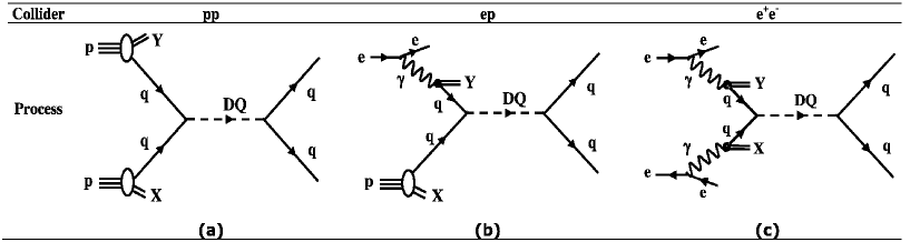
Figure 1: Schematic presentation of resonant production of scalar or vector diquarks at three types of colliders: a) $pp$ collisions, b) $ep$ collisions with one resolved photon process and c) $e^{+}e^{-}$ collisions with two resolved photon process.

II Interaction Lagrangian

A model independent, baryon number conserving, most general $SU(3)_{C}\times SU(2)_{W}\times U(1)_{Y}$ invariant effective lagrangian for scalar and vector diquarks has the form Atag98 ; Arik02

$$L_{|B|=0} =f_{1L}\overline{q}_{L}\gamma^{\mu}q_{L}DQ_{1\mu}^{c}+(f_{1R}\overline{d}_{R}\gamma^{\mu}d_{R}+f_{1R}^{\prime}\overline{u}_{R}\gamma^{\mu}u_{R})DQ_{1\mu}^{\prime c}$$

$$+\widetilde{f}_{1R}\overline{u}_{R}\gamma^{\mu}d_{R}\widetilde{DQ}_{1\mu}^{c}+f_{3L}\overline{q}_{L}\mathbf{\tau}\gamma^{\mu}q_{L}\cdot\mathbf{DQ}_{3\mu}^{c}$$

$$+f_{2}\overline{q}_{L}i\tau_{2}u_{R}DQ_{2}^{c}+\widetilde{f}_{2}\overline{q}_{L}i\tau_{2}d_{R}\widetilde{DQ}_{2}^{c}+\text{H.c.}$$ (4)

$$L_{|B|=2/3} =(g_{1L}\overline{q}_{L}^{c}i\tau_{2}q_{L}+g_{1R}\overline{u}_{R}^{c}d_{R})DQ_{1}^{c}+\widetilde{g}_{1R}\overline{d}_{R}^{c}d_{R}\widetilde{DQ}_{1}^{c}$$

$$+\widetilde{g}_{1R}^{\prime}\overline{u}_{R}^{c}u_{R}\widetilde{DQ}_{1}^{\prime c}+g_{3L}\overline{q}_{L}^{c}i\tau_{2}\mathbf{\tau}q_{L}\cdot\mathbf{DQ}_{3}^{c}$$

$$+g_{2}\overline{q}_{L}^{c}\gamma^{\mu}d_{R}DQ_{2\mu}^{c}+\widetilde{g}_{2}\overline{q}_{L}^{c}\gamma^{\mu}u_{R}\widetilde{DQ}_{2\mu}^{c}+\text{ H.c.}$$ (5)

where the $|B|=0$ diquarks are familiar fields, as they resemble the electroweak gauge vectors, and the neutral and charged Higgs scalars. Here, we consider only the $|B|=2/3$ diquarks. In Eq. (4) and (5), $q_{L}=(u_{L},d_{L})$ denotes the left handed quark spinor and $q^{c}=C\bar{q}^{T}$ ($\bar{q}^{c}=-q^{T}C^{-1}$) is the charge conjugated quark field. Following Atag98 ; Arik02 , the possible scalar and vector diquarks are $SU(3)_{C}$ anti-triplets and sextets. For the sake of simplicity, color and generation indices are ommitted in (4) and (5). Scalar diquarks $DQ_{1}$, $\widetilde{DQ}_{1}$, $\widetilde{DQ}_{1}^{\prime}$ are $SU(2)_{W}$ singlets and $\mathbf{DQ}_{3}$ is $SU(2)_{W}$ triplet. Vector diquarks $DQ_{2}$ and $\widetilde{DQ}_{2}$ are $SU(2)_{W}$ doublets. At this stage, we assume that each SM generation has its own diquarks and couplings in order to avoid flavour changing neutral currents (FCNC). Furthermore, the members of a given multiplet are assumed to be the mass degenerated. A general classification of the first generation, color anti-triplet ($\mathbf{3}^{\ast}\mathbf{)}$ diquarks is shown in Table 2.

Table 2: Quantum numbers of the first generation, color $\bar{3}$ diquarks described by the effective lagrangian in the text according to $SU(3)_{C}\times SU(2)_{W}\times U(1)_{Y}$ invariance where the hypercharge $Y=2(Q-I_{3})$.

	SU(3)C	SU(2)W	U(1)Y	$Q$	Couplings
Scalar Diquarks
$DQ_{1}$	3⋆	1	2/3	1/3	$u_{L}d_{L}(g_{1L}),\,u_{R}d_{R}(g_{1R})$
$\widetilde{DQ}_{1}$	3⋆	1	-4/3	2/3	$d_{R}d_{R}(\tilde{g}_{1R})$
$\widetilde{DQ}_{1}^{\prime}$	3⋆	1	8/3	4/3	$u_{R}u_{R}(\tilde{g}_{1R}^{\prime})$
$DQ_{3}$	3⋆	3	2/3	$\left(\begin{array}[c]{c}4/3\\ 1/3\\ -2/3\end{array}\right)$	$\left(\begin{array}[c]{c}u_{L}u_{L}(\sqrt{2}g_{3L})\\ \begin{array}[c]{c}u_{L}d_{L}(-g_{3L})\\ d_{L}d_{L}(-\sqrt{2}g_{3L})\end{array}\end{array}\right)$
Vector Diquarks
$DQ_{2\mu}$	3⋆	2	-1/3	$\left(\begin{array}[c]{c}1/3\\ -2/3\end{array}\right)$	$\left(\begin{array}[c]{c}d_{R}u_{L}(g_{2})\\ d_{R}d_{L}(-g_{2})\end{array}\right)$
$\widetilde{DQ}_{2\mu}$	3⋆	2	5/3	$\left(\begin{array}[c]{c}4/3\\ 1/3\end{array}\right)$	$\left(\begin{array}[c]{c}u_{R}u_{L}(\tilde{g}_{2})\\ u_{R}d_{L}(-\tilde{g}_{2})\end{array}\right)$

For the present analysis, we consider the color $\mathbf{3}^{\ast}$ scalar $DQ_{1}$ or $DQ_{3}^{0}$ diquarks coupled to $ud$ pairs, $\widetilde{DQ}_{1}$ or $DQ_{3}^{-}$ diquarks coupled to $dd$ pair and $\widetilde{DQ}_{1}^{\prime}$ or $DQ_{3}^{+}$ diquarks coupled to $uu$ pair. The vector diquarks $DQ_{2}^{1}$ and $\widetilde{DQ}_{2}^{2}$ of type $ud$, $DQ_{2}^{2}$ of type $dd$ and $\widetilde{DQ}_{2}^{1}$ of type $uu$ are considered. The interaction between the diquark and quark pair is described by the effective lagrangian (5) with different couplings.

III Decay Widths

For the decay width calculation, we take the coupling as $g_{DQ}^{2}=g_{L}^{2}+g_{R}^{2}$ for each diquark type. For numerical results, we will use the definition $g_{DQ}^{2}=4\pi\alpha_{DQ}$ when only one type of coupling assumed to be nonzero. Diquarks decay into quark pairs, and the decay width $\Gamma_{DQ}$ derived from the same lagrangian is

$$\Gamma_{DQ}^{S} ={\frac{F_{S}g_{DQ}^{2}m_{DQ}}{16\pi}}\simeq 25\,\text{GeV}({\frac{F_{S}m_{DQ}}{{1\,\text{TeV}}}})\;\;\;\text{\mbox{for}}\;\;\alpha_{DQ}=0.1$$ (6)

$$\Gamma_{DQ}^{V} ={\frac{F_{S}g_{DQ}^{2}m_{DQ}}{24\pi}}\simeq 17\text{GeV}({\frac{F_{S}m_{DQ}}{{1\,\text{TeV}}}})\;\;\;\text{\mbox{for}}\;\;\alpha_{DQ}=0.1$$ (7)

where $F_{S}$ contains the color factor for a representation including the statistical factors associated with the presence of identical fermions in the final state, and $m_{DQ}$ is the mass of scalar ($S$) or vector ($V$) diquark.

IV Signal and Background

The signal for diquark production would clearly manifest itself in two jets cross sections. The differential cross section for any type of scalar and vector diquark resonant production can be written as follows

$${\frac{d\hat{\sigma}^{S}}{d\hat{t}}}(q_{i}q_{j} \rightarrow DQ\rightarrow q_{i}q_{j})={\frac{F{{}_{S}g}_{DQ}^{4}}{64\pi[(\hat{s}-m_{DQ}^{2})^{2}+(m_{DQ}\Gamma_{DQ}^{S})^{2}]}}$$ (8)

$${\frac{d\hat{\sigma}^{V}}{d\hat{t}}}(q_{i}q_{j} \rightarrow DQ\rightarrow q_{i}q_{j})={\frac{F{{}_{S}g}_{DQ}^{4}(\hat{t}^{2}+\hat{u}^{2})}{16\pi\hat{s}^{2}[(\hat{s}-m_{DQ}^{2})^{2}+(m_{DQ}\Gamma_{DQ}^{V})^{2}]}.}$$ (9)

In the narrow width approximation ($\Gamma_{DQ}/m_{DQ}<0.1$), the cross section of the $s-$channel diquark production can be obtained as

$${\hat{\sigma}}_{R}^{S}(\widehat{s}) \simeq\frac{F{{}_{S}g}_{DQ}^{4}\widehat{s}}{64m_{DQ}\Gamma_{DQ}^{S}}\delta(\widehat{s}-m_{DQ}^{2})$$ (10)

$${\hat{\sigma}}_{R}^{V}(\widehat{s}) \simeq\frac{F{{}_{S}g}_{DQ}^{4}\widehat{s}}{48m_{DQ}\Gamma_{DQ}^{V}}\delta(\widehat{s}-m_{DQ}^{2})$$ (11)

where $\widehat{s}$ is the Mandelstam variable corresponding to the square of center-of-mass energy for the subprocess.

IV.1 pp Collider

The total cross section for the resonance production of scalar diquarks at $pp$ collider is given by

$$\sigma=\int_{m_{DQ}^{2}/s}^{1}\frac{dx}{x}f_{q/p}(x,Q_{p}^{2})f_{q^{\prime}/p}(m_{DQ}^{2}/xs,Q_{p}^{2})\widehat{{\sigma}}(\widehat{s})$$ (12)

where $f_{q/p}(x,Q_{p}^{2})$ and $f_{q^{\prime}/p}(x,Q_{p}^{2})$ correspond to the quark distribution functions from the proton and we have used CTEQ5L CTEQ5L parametrization with $Q_{p}^{2}=\widehat{s}$. As a consequence of this energy scan there will be quarks whose energies adequate for the resonance production of diquarks. The cross section is plotted against the diquark mass in Fig. 2 (a-b) for LHC energy ($\sqrt{s}=14$ TeV) and coupling $\alpha_{DQ}=0.1$. From these figures we find that diquarks with charge $|Q|=4/3$ have the largest cross sections when compared to the other types.

(a)                                                            (b)

Figure 2: Total cross sections in $pp$ collisions for a) scalar and b) vector diquarks for different charges, with coupling strength $\alpha_{DQ}=0.1$, depending on their masses.

The scalar and vector diquarks will decay via $DQ\rightarrow q_{i}q_{j}.$ Therefore, the relevant signal will be a pair of hard jets in the final state. At the LHC energy, major QCD background processes contributing to two-jets ($2j$) final states and their integrated cross sections are given in Table 3.

Table 3: The cross sections (in pb) for QCD backgrounds contributing to two jets final states at parton level generated by CompHEP with various $p_{T}$ cuts.

Process		$p_{T}>0.1$ TeV		$p_{T}>0.5$ TeV		$p_{T}>1$ TeV		$p_{T}>2$ TeV
$gg\rightarrow gg$		6.3$\times 10^{5}$		2.0$\times 10^{2}$		2.3$\times 10^{0}$		5.7$\times 10^{-3}$
$qg\longrightarrow qg$		6.4$\times 10^{5}$		4.8$\times 10^{2}$		1.0$\times 10^{1}$		5.7$\times 10^{-2}$
$qq^{\prime}\rightarrow qq^{\prime}$		1.0$\times 10^{5}$		1.8$\times 10^{2}$		6.7$\times 10^{0}$		8.8$\times 10^{-2}$
$gg\rightarrow q\overline{q}$		2.4$\times 10^{4}$		9.8$\times 10^{0}$		1.0$\times 10^{-1}$		2.9$\times 10^{-4}$
$q\overline{q}\longrightarrow q^{\prime}\overline{q^{\prime}}$		1.6$\times 10^{3}$		2.8$\times 10^{0}$		1.3$\times 10^{-1}$		1.1$\times 10^{-3}$
$q\overline{q}\longrightarrow gg$		1.5$\times 10^{3}$		2.5$\times 10^{0}$		6.7$\times 10^{-2}$		8.5$\times 10^{-4}$
Total		1.4$\times 10^{6}$		8.8$\times 10^{2}$		1.9$\times 10^{1}$		1.5$\times 10^{-1}$

The values in Table 3 have been generated by CompHEP program comphep at parton level with various $p_{T}$ cuts on the jets. It is clear that higher $p_{T}$ cuts reduce the background cross sections significantly. These $p_{T}$ cuts can be translated into the rapidity cuts according to the relation between the $p_{T}$ of a jet and the rapidity with $p_{T}=m_{jj}/2\cosh y.$ Standard kinematic relations for the invariant mass $m_{jj}$ and $p_{T}$ distributions of two-jet final states can be found in Atag98 ; Arik02 . Figure 3 shows the dijet invariant mass distribution for the process $pp\rightarrow 2j+X$ including the signal and the QCD backgrounds at the LHC. For comparison signal peaks for scalar and vector diquark masses $m_{DQ}=1,3,5,7,9$ TeV and $\alpha_{DQ}=0.1$ are shown on the smooth background distribution.

Figure 3: Dijet invariant mass distributions for $pp\rightarrow 2jX.$ Resonance peaks are shown for scalar and vector diquark masses 1, 3, 5, 7, and 9 TeV for comparison with smooth QCD backgrounds.

In order to obtain the observability of diquarks at LHC we have calculated signal (S) and background (B) event estimations for an integrated luminosity of $10^{5}$ pb^-1. The signal generated by a diquark of mass $m_{DQ}$ and decay rate $\Gamma_{DQ}$ is calculated integrating the differential cross section in the two-jet invariant mass interval $m_{DQ}-\Gamma_{DQ}<m_{jj}<m_{DQ}+\Gamma_{DQ}$ which embraces approximately $95\%$ of the events around the resonance. For a realistic analysis of the background events we take into account the finite energy resolution of the LHC-ATLAS hadronic calorimeter ATLAS as $\delta E/E=0.5/\sqrt{E}+0.03$ for jets with $|y|<3.$ The corresponding two-jet invariant mass resolution is given approximately by $\delta m_{jj}=0.5\sqrt{m_{jj}}+0.02m_{jj}$. The background is calculated by integrating the cross sections in the range $m_{DQ}-\Delta m<m_{jj}<m_{DQ}+\Delta m$ with $\Delta m=\max(\Gamma_{DQ},\delta m_{jj})$. The significance of signal over background is defined as $S/\sqrt{B}.$ In Fig. 4 we present $S/\sqrt{B}$ as a function of the diquark mass for the scalar and vector diquarks with charges $|Q|=4/3$ and $2/3.$

Figure 4: The signal significances $S/\sqrt{B}$ for diquarks as a function of diquark mass $m_{DQ}$ at the LHC.

If we take at least $25$ signal events and $S/\sqrt{B}\geq 5$ as discovery criteria, scalar (vector) diquarks with charge $|Q|=2/3$ can be observed up to $7.5$ ($8.5$) TeV. For the diquarks with charge $|Q|=4/3$ it is possible to cover mass ranges up to $9.5$ ($10)$ TeV at the LHC with $L_{int}=10^{5}$ pb^-1. For this luminosity, $10^{7}$ scalar diquark events/year and $10^{8}$ vector diquark events/year are expected for $m_{DQ}=1$ TeV. Our results show that even for much lower coupling constants as $10^{-3}$, diquarks should be seen at the LHC.

IV.2 ep collider

In order to calculate the total cross section for diquark production due to resolved photon process at $ep$ colliders, we use the formula

$$\sigma=\int_{m_{DQ}^{2}/s}^{1}\frac{dx}{x}\int_{x}^{1}\frac{dy}{y}f_{\gamma/e}(y)f_{q^{\prime}/\gamma}(x/y,Q_{\gamma}^{2})f_{q/p}(m_{DQ}^{2}/xs,Q_{p}^{2})\widehat{{\sigma}}(\widehat{s})$$ (13)

where $f_{\gamma/e}(y)$ Florian99 and $f_{q^{\prime}/\gamma}(x/y,Q_{\gamma}^{2})$ Gluck92 corresponds to the photon energy spectrum and the probability density of finding a quark ($q\prime$) carrying a fraction $x/y$ of the energy of the electrons in the initial beams, respectively. In (13) the integrals over the momentum fractions $x$ and $y$ are the mathematical representation of an energy scan performed by the partons coming from photons and protons. We use the photon spectrum $f_{\gamma/e}(y)$ resulting from bremsstrahlung Florian99 with the electron beam energy $E_{e}$

$$f_{\gamma/e}(y)=\frac{\alpha}{2\pi}\left[\frac{1+(1-y)^{2}}{y}\ln\frac{4E_{e}^{2}(1-y)^{2}}{m_{e}^{2}y^{2}}+2m_{e}^{2}y\left(\frac{1}{4E_{e}^{2}(1-y)}-\frac{1-y}{m_{e}^{2}y^{2}}\right)\right].$$ (14)

We present the cross sections for scalar diquarks against their masses for coupling $\alpha_{DQ}=0.1$ and charges $|Q|=4/3,1/3$ and $2/3$ using the bremsstrahlung process in Fig. 5 at CLIC$\otimes$LHC based $ep$ colliders with $\sqrt{s_{ep}}=6.48$ TeV.

Figure 5: The total cross sections for the process $ep\rightarrow DQ+X\rightarrow 2j+X$ at $\sqrt{s_{ep}}=6.48$ TeV depending on the mass of scalar diquarks.

In order to see the potentials of possible options of $ep$ colliders with different center of mass energies, we plot diquark production cross sections depending on the $\sqrt{s_{ep}}$. As seen from the Fig. 6 vector diquarks have larger cross sections than the scalar for the considered center of mass energy region. In principle, the vector and scalar type diquarks can be easily distinguished by the angular distribution of produced jets, the electric charge of diquarks can be determined by the interactions with photon.

Figure 6: The production cross sections $\sigma(ep\rightarrow DQ+X\rightarrow 2j+X)$ for scalar and vector diquarks with charge $|Q|=4/3$ and coupling $\alpha_{DQ}=0.1$ depending the center of mass energy of the $ep$ colliders.

In the resonant production mechanism of diquarks with resolved photon process in collision $ep\rightarrow DQ+X\rightarrow 2j+X$, most of the partcles in the final state are expected to be lost in the beam pipe, the two exceptions being the quarks resulting from diquark decay. As a result, the relevant signal is a $p_{T}$ balanced coplanar pair of jets and it will contain two hard jets in the final state. All the relevant interactions with the diquarks are implemented into the CompHEP comphep program. The decay width of diquarks and the cross sections for signal and background processes are calculated with this program.

In order to study contributing backgrounds we need to take into account all the diagrams contributing to two-jets final states. The process $ep\rightarrow 2j+X$ has potentially large QCD background. At the $ep$ colliders, major processes contributing to two-jets ($2j$) final states and their integrated cross sections are given in Table 4.

Table 4: The major processes contributing to two jet ($jj$) final states with a cut $p_{T}>100$ GeV at the $ep$ collisions with different center of mass energy $\sqrt{s_{ep}}$.

Collider		ILC$\otimes$LHC		CLIC$\otimes$LHC
$\sqrt{s_{ep}}$(TeV)		2.64		3.74		6.48
$\gamma\overline{q}\rightarrow g\overline{q}$		$2.631\times 10^{0}$		$5.064\times 10^{0}$		$1.234\times 10^{1}$
$\gamma q\rightarrow gq$		$8.275\times 10^{0}$		$1.257\times 10^{1}$		$2.290\times 10^{1}$
$\gamma g\rightarrow q\overline{q}$		$1.522\times 10^{1}$		$3.248\times 10^{1}$		$9.233\times 10^{1}$
Total		$2.613\times 10^{1}$		$5.011\times 10^{1}$		$1.276\times 10^{2}$

The values in Table 4 have been generated by CompHEP at parton level for transverse momentum cut of the jets $p_{T}>100$ GeV. Fig. 7 shows jet-jet invariant mass distribution for the process $ep\rightarrow 2jX$ at CLIC$\otimes$LHC based $ep$ collider with $\sqrt{s_{ep}}=6.48$ TeV.

Figure 7: The invariant mass distributions for the QCD background with the inclusion of scalar diquark signals at $ep$ collisons.

In our analysis, we determine the expected significance of the signal over background for collider parameters given in Table 1 for $ep$ colliders. It is convenient to collect the data in two-jet invariant mass bins since the signal is concentrated in a small region of the invariant mass spectrum. Therefore, we introduced the cut $\mid m_{jj}-$ $m_{DQ}\mid\leq 25$ GeV which is efficient only for diquark masses between 0.5 and 1 TeV. For heavier diquarks rather broad resonances are expected and the cut $\mid m_{jj}-$ $m_{DQ}\mid\leq 50$ GeV becomes suitable for $1$ TeV$<m_{DQ}<2.5$ TeV. This range of the invariant mass will embrace approximately $95\%$ of the signal events around the diquark resonance. For a realistic analysis we have estimated background events for $ep$ colliders with the integrated luminosity of $10^{3}$ pb^-1 taking into account the energy resolution of the hadronic calorimeter. The statistical significances $S/\sqrt{B}$ of diquark signal over background are shown in Fig. 8 for ILC$\otimes$LHC and CLIC$\otimes$LHC based $ep$ colliders. From Fig. 8, we find that scalar (vector) diquarks can be seen up to $1$ ($1.6$) TeV at the $ep$ collider with $\sqrt{s}=6.48$ TeV. A slightly lower limits can be obtained for the other $ep$ options.

Figure 8: The signal significances $S/\sqrt{B}$ as a function of scalar and vector diquark mass $m_{DQ}$ at different $ep$ collider energies.

If we take into account the integrated luminosity $L=10^{3}$ pb^-1 for the CLIC$\otimes$LHC based $ep$ collider with $\sqrt{s}=6.48$ TeV, $44$ scalar diquark events and $264$ vector diquark events/year are expected for $m_{DQ}=1$ TeV and $\alpha_{DQ}=0.1$.

IV.3 e⁺e^- collider

The cross section for the production of a pair of jets through the two resolved photon process is given by

$$\sigma=\int_{x_{\min}}^{x_{\max}}dx\int_{y_{\min}}^{y_{\max}}dyf_{q/e}(x,Q_{\gamma}^{2})f_{q^{\prime}/e}(y,Q_{\gamma}^{2})\widehat{{\sigma}}(\widehat{s})$$ (15)

here $f_{q/e}(x,Q_{\gamma}^{2})$ and $f_{q^{\prime}/e}(y,Q_{\gamma}^{2})$ correspond to the probability density of finding a quark $q$ and $q^{\prime}$ carrying a fraction $x$ and $y$ of the energy of the electrons and positrons in the initial beams, respectively. In (15) the integrals over the momentum fractions $x$ and $y$ are the mathematical representation of an energy scan performed by the partons coming from electrons and positrons. The lower limits of the integrations guarantee the energy required for the production of quarks. As a consequence of this energy scan there will be quarks whose energies adequate for the resonance production of diquarks. For the probability $f_{q/e}(x,Q_{\gamma}^{2})$ resulting from the convolution of the spectrum of photons $f_{\gamma/e}(x_{2})$ converted from the initial beams and photonic parton distribution function $f_{q/\gamma}(x_{1},Q_{\gamma}^{2})$ Gluck92 , we use

$$f_{q/e}(x,Q_{\gamma}^{2}) =\int_{x_{2\min}}^{x_{2\max}}dx_{2}\int_{x_{1\min}}^{x_{1\max}}dx_{1}f_{\gamma/e}(x_{2})f_{q/\gamma}(x_{1},Q_{\gamma}^{2})\delta(x_{1}x_{2}-x)$$ (16)

$$=\int_{x}^{1}\frac{dx_{2}}{x_{2}}f_{\gamma/e}(x)f_{q/\gamma}(\frac{x}{x_{2}},Q_{\gamma}^{2})$$ (17)

For the relevant $Q_{\gamma}^{2}$ value entering the parton distribution in the photon, we have taken $Q_{\gamma}=\sqrt{\widehat{s}}/2.$

In Fig. 9, the quark probability density function $f_{q/e}(x,Q_{\gamma}^{2})$ within electron beam are presented for bremsstrahlung photons at beam energy $E_{e}=1.5$ TeV.

Figure 9: The probability density for up ($u)$ and down ($d)$ quarks within electron beam for bremsstrahlung photons.

Here, we show only $u$ and $d$ quark distributions in photon since we deal with only the first family diquarks. In Fig. 10 (a-b), the production cross section versus scalar and vector diquark mass is plotted for $e^{+}e^{-}$ with the center of mass energy $\sqrt{s_{e^{+}e^{-}}}=0.5,1$ and $3$ TeV.

(a)                                                            (b)

Figure 10: The production cross sections for (a) scalar diquark and (b) vector diquark with charge $|$$Q|=4/3$ at $e^{+}e^{-}$ colliders with $\sqrt{s_{e^{+}e^{-}}}=0.5,1$ and $3$ TeV, where the coupling $\alpha_{DQ}=0.1$.

The two-jet background receives contributions from the annihilation process $e^{+}e^{-}\rightarrow\gamma,Z\rightarrow q\overline{q}$ and the hard two photon processes. The two photon processes can be of type direct, one resolved and two resolved. The last two processes, despite being higher order in $\alpha_{s},$ contribute significantly at lower energies. The spectrum of initial state radiation (ISR, photon radiation from the incoming electrons and positrons) contains the ISR scale inherent to the process under consideration Kuraev85 . In our calculations, this spectrum is taken into account using the CompHEP program with the convolution of beamstrahlung spectra. Beamstrahlung is the process of energy loss by the incoming electron/positron in the field of the positron/electron bunch moving in the opposite direction. Beamstrahlung spectrum is an attribute of the linear collider design and depends on the bunch geometry, bunch charge and the collision energy. The photon spectrum resulting from the electromagnetic interaction between the electron and positron beams in the intersection region is described by a more complicated expression Chen92 . The beamstrahlung parameters, $\Upsilon$ and $N_{\gamma}$, which in their turn are determined by the bunch design of a linear collider:

$$\Upsilon={\frac{5\alpha NE_{e}}{6m_{e}^{3}\sigma_{z}(\sigma_{x}+\sigma_{y})}}\quad,\qquad N_{\gamma}={\frac{25\alpha^{2}N}{12m_{e}(\sigma_{x}+\sigma_{y})}}{\frac{1}{\sqrt{1+\Upsilon^{2/3}}}}$$ (18)

where $N$ is the number of particles in the bunch; $E_{e}$ and $m_{e}$ are the energy and mass of the electron, respectively; $\sigma_{x},\sigma_{y}$ and $\sigma_{z}$ are the average sizes of the particle bunches. We presented the beamstrahlung parameters in Table  5 and their effects in the background calculations in Table  6.

Table 5: Collider parameters relevant for the calculation of beamstrahlung. $\Upsilon$ is the beamstrahlung parameter and $N_{\gamma}$ is the average number of photons per electron.

Collider		ILC		CLIC
parameter		500 GeV		1 TeV		3 TeV
N(1010)		2		0.4		0.4
$\sigma_{x}($nm$)$		655		115		43
$\sigma_{y}($nm$)$		5.7		1.75		1
$\sigma_{z}(\mu$m$)$		300		30		30
$\Upsilon$		0.045		1.014		8.068
$N_{\gamma}$		1.22		1.04		1.74

Table 6: Background calculation with the ISR and beamstrahlung effects. The numbers are the cross sections in pb for the process $e^{+}e^{-}\rightarrow\gamma,Z\rightarrow q\bar{q}$ with $p_{T}^{j}>20$ GeV ($p_{T}^{j}>100$ GeV).

Collider		ILC		CLIC
parameter		500 GeV		1 TeV		3 TeV
no ISR		2.22(1.96)		0.546(0.672)		0.0604(0.0602)
with ISR		8.16(2.11)		1.96(0.629)		0.276(0.0829)
with ISR+beamstrahlung		8.38(2.16)		4.30(1.04)		67.55(1.39)

We determine the expected significance of the signal over the background for collider parameters as given in Table 1, for ILC operating at 500 GeV, CLIC operating at 1 and 3 TeV. For the realistic analysis of the background we consider the generic hadron calorimeters with the two-jet mass resolution $\delta m_{jj}=0.5\sqrt{m_{jj}}+0.03m_{jj}.$ In order to reduce the background we vetoed events exhibiting $Z$-bosons decaying into two-jets through the cut $m_{jj}>100$ GeV. In Fig. 11, we presented the contributions from both the annihilation process with/without ISR+beamstrahlung and two-photon processes to dijet cross sections at $\sqrt{s_{e^{+}e^{-}}}=3$ TeV.

Figure 11: The transverse momentum distributions of the jet.

We conclude that signal significances scale with the collider luminosity as $\sqrt{L},$ and higher luminosities are desirable for a good signal over background discrimination. In determining the background events we considered some cuts on transverse momentum $p_{T}>100$ GeV of the jets. In Fig. 12, we present the signal significance that can be reached at $e^{+}e^{-}$ collider with at $\sqrt{s_{e^{+}e^{-}}}=3$ TeV.

Figure 12: The scalar and vector diqurk signal significance as a function of their masses.

We take the indication of signal $S/\sqrt{B}\geq 3$ and find that vector diquarks can be probed up to $1$ TeV at $e^{+}e^{-}$ collider with $\sqrt{s_{e^{+}e^{-}}}=3$ TeV. For the $e^{+}e^{-}$ colliders running at the center of mass energy of $1$ TeV we can search for scalar diquarks up to $325$ GeV and vector diquarks up to $375$ GeV.

V Conclusion

The resonant production of scalar and vector diquarks at LHC have large cross section. With reasonable cuts, it may be possible to cover mass ranges up to $10$ TeV for coupling $\alpha_{D}=0.1$. For smaller couplings as $\alpha_{D}=10^{-3}$, it is still possible to probe diquarks up to the mass of $4$ TeV at an integrated luminosity $L=10^{2}$fb^-1. We find that vector diquarks can be seen up to $1.6$ TeV at the $ep$ collider with $\sqrt{s}=6.48$ TeV and a slightly lower limits can be obtained for scalar diquarks. The two hard photon processes prevail at energies below $\sqrt{s}/2$ while the annihilation prevails at higher energies. Therefore, the attainable mass limits for diquarks are smaller than $\sqrt{s}/2$ at linear colliders with the parameters given in Table 1.

A limited number of measurements of diquark properties can be carried out at the hadron colliders. The future high energy linear $e^{+}e^{-}$ colliders and linac-ring type $ep$ colliders based on the hadron and lepton colliders would complement the measurements performed at hadron colliders. The resolved photon contributions to the search for new physics becomes important for forthcoming $ep$ and $e^{+}e^{-}$ collisions.

- (1) J. Wudka, Phys. Lett. B 167 (1986) 337.
- (2) J. L. Hewett and T.G. Rizzo, Phys. Rep. 183 (1989) 193.
- (3) F. Abe et al., CDF Collaboration, Phys. Rev. D. 55 (1997) R5263; T. Dorigo, FERMILAB-CONF-97-281-E, CDF-PUB-EXOTIC-PUBLIC-4238, (unpublished) (1997).
- (4) G. Bhattacharyya, D. Choudury and K. Sridhar, Phys. Lett. B 355, (1995) 193.
- (5) A. Gusso, J. Phys. G: Nucl. Part. Phys. 30, (2004) 691.
- (6) V. D. Angelopoulos et al., Nucl. Phys. B 292, (1987) 59.
- (7) E. N. Argyres, C. G. Papadopoulos, S. D. P. Vlassopoulos, Phys. Lett. B 202, (1988) 425.
- (8) S. Atağ, O. Çakır, and S. Sultansoy, Phys. Rev. D 59, (1999) 015008.
- (9) E. Arik, S. A. Cetin, O. Çakır, S. Sultansoy, J. High Energy Phys. JHEP09 (2002) 024.
- (10) T. G. Rizzo, Z. Phys. C 43, (1989) 223.
- (11) P. Abreu et al., DELPHI Collaboration, Phys. Lett. B 446, 62 (1999).
- (12) Stefan Soldner-Rembold et al., OPAL Collaboration, 18th International Symposium On Lepton And Photon Interactions (LP 97) 28 Jul - 1 Aug 1997, Hamburg, Germany; hep-ex/9706003.
- (13) M.A. Doncheski and S. Godfrey, Phys. Rev. D 49, 6220 (1994); ibid. 51, 1040 (1995); Phys. Lett. B 393, 355 (1997); Mod. Phys. Lett. A 12, 1719 (1997).
- (14) H. L. Lai et al., CTEQ Collaboration, Eur.Phys. J. C 12, (2000) 375.
- (15) E.Boos et al., CompHEP Collaboration, CompHEP 4.4: Automatic computations from Lagrangians to events, Nucl. Instrum. Meth. A534(2004), p250, hep-ph/0403113; COMPHEP - a package for evaluation of Feynman diagrams and integration over multi-particle phase space. User’s manual for version 3.3, hep-ph/9908288.
- (16) ATLAS Collaboration, Detector and Physics Performance Technical Design Report, Volume 1, ATLAS TDR 14, CERN/LHCC 99-14, (1999) and Volume 2, ATLAS TDR 15, CERN/LHCC 99-15, (1999).
- (17) D. de Florian, S. Frixione, Phys. Lett. B 457, (1999) 236.
- (18) M. Gluck, E. Reya, A. Vogt, Phys. Rev. D 46, (1992) 1973.
- (19) E.A. Kuraev and V.S. Fadin, Sov. J. Nucl. Phys. 41, 466 (1985).
- (20) P. Chen, Phys. Rev. D 46, 1186 (1992).