hep-ph/0508198

CERN-PH-TH/2005-111, UMN–TH–2404/05, FTPI–MINN–05/19

Supersymmetric Benchmarks with Non-Universal Scalar Masses or Gravitino Dark Matter

A. De Roeck¹, J. Ellis¹, F. Gianotti¹, F. Moortgat¹, K. A. Olive² and L. Pape^{1,3 1}Physics Department, CERN, CH-1211 Geneva 23, Switzerland
²William I. Fine Theoretical Physics Institute, University of Minnesota, Minneapolis, MN 55455, USA
³Department of Physics, ETHZ, CH-8093 Zurich, Switzerland

Abstract

We propose and examine a new set of benchmark supersymmetric scenarios, some of which have non-universal Higgs scalar masses (NUHM) and others have gravitino dark matter (GDM). The scalar masses in these models are either considerably larger or smaller than the narrow range allowed for the same gaugino mass $m_{1/2}$ in the constrained MSSM (CMSSM) with universal scalar masses $m_{0}$ and neutralino dark matter. The NUHM and GDM models with larger $m_{0}$ may have large branching ratios for Higgs and/or $Z$ production in the cascade decays of heavier sparticles, whose detection we discuss. The phenomenology of the GDM models depends on the nature of the next-to-lightest supersymmetric particle (NLSP), which has a lifetime exceeding $10^{4}$ seconds in the proposed benchmark scenarios. In one GDM scenario the NLSP is the lightest neutralino $\chi$, and the supersymmetric collider signatures are similar to those in previous CMSSM benchmarks, but with a distinctive spectrum. In the other GDM scenarios based on minimal supergravity (mSUGRA), the NLSP is the lighter stau slepton ${\tilde{\tau}}_{1}$, with a lifetime between $\sim 10^{4}$ and $3\times 10^{6}$ seconds. Every supersymmetric cascade would end in a ${\tilde{\tau}}_{1}$, which would have a distinctive time-of-flight signature. Slow-moving ${\tilde{\tau}}_{1}$’s might be trapped in a collider detector or outside it, and the preferred detection strategy would depend on the ${\tilde{\tau}}_{1}$ lifetime. We discuss the extent to which these mSUGRA GDM scenarios could be distinguished from gauge-mediated models.

CERN-PH-TH/2005-111

August 2005

1 Introduction

Among the most promising prospects for new physics that might be discovered at the LHC is supersymmetry. Its appearance at the TeV energy scale is motivated by the stability of the mass hierarchy [1], the lightness of the Higgs boson as inferred from precision electroweak measurements [2], the possibility of unifying the gauge interactions [3], and (assuming that $R$-parity is conserved) the existence of a natural candidate for cold dark matter (CDM) [4]. However, despite these phenomenological hints and the intrinsic beauty of supersymmetry, there is no direct evidence for its existence. Evidence for new physics at the TeV scale might be provided by the anomalous magnetic moment of the muon, $g_{\mu}-2$, if it is confirmed that measurements are significantly different from the Standard Model prediction [5]. Supersymmetry could be one of the possible interpretations, but not the only one.

In advance of experiments at the LHC and other accelerators intended to explore the TeV energy range in more detail, it is valuable to understand the variety of possible signatures of supersymmetry, taking into account the constraints imposed by present accelerator experiments as well as astrophysics and cosmology. Experimental signatures of supersymmetry depend quite sensitively on the possible sparticle masses, which in turn depend on the unknown mechanism of supersymmetry breaking. There have already been a number of surveys of the supersymmetric parameter space [6, 7, 8, 9], some focusing on specific benchmark points that exemplify distinct possibilities, and others tracking the phenomenological variations along lines in this space that are consistent with the cosmological and other constraints.

Most such studies have focused on the CMSSM, in which the supersymmetry-breaking gaugino, scalar and trilinear parameters $m_{1/2},m_{0}$ and $A_{0}$, respectively, are each assumed to be universal at some input GUT scale $\sim 10^{16}$ GeV, and the gravitino is assumed not to be the lightest supersymmetric particle (LSP). However, this is not the only possibility: universality is not strongly favoured within our current understanding of possible underlying theoretical frameworks such as string theory, and the gravitino might be the LSP. Therefore, in this paper we investigate benchmark scenarios that sample models with patterns of supersymmetry breaking different from that in the CMSSM.

The most dubious of the CMSSM universality assumptions may be that for the soft supersymmetry-breaking scalar masses $m_{0}$. Universality between sparticles in the same gauge multiplet is inevitable, and universality between sparticles in different generations that share the same quantum numbers is motivated by constraints from flavour-changing neutral interactions [10]. Moreover, sparticles with different quantum numbers may originate from common GUT multiplets, in which case their soft supersymmetry-breaking scalar masses should also be universal at the GUT scale, apart from possible non-universal GUT $D$ terms. However, none of these arguments give any reason why the soft supersymmetry-breaking scalar masses of the electroweak Higgs multiplets should be universal, and this may be the Achilles heel of the CMSSM. Accordingly, some of the non-CMSSM scenarios we study in this paper have non-universal Higgs masses (NUHM) [11, 12].

We assume in this paper that $R$-parity is conserved, so that the LSP is stable and a candidate for the CDM required by astrophysics and cosmology [4]. However, even if one accepts the CMSSM universality assumptions, it is not evident that the LSP is necessarily the lightest neutralino $\chi$, as usually assumed in CMSSM analyses. Another plausible candidate is the gravitino [13] - [16], the supersymmetric partner of the graviton, in which case options for the next-to-lightest supersymmetric particle (NLSP) include the lightest neutralino and the lighter stau slepton ${\tilde{\tau}}_{1}$. The gravitino mass $m_{3/2}$ is poorly constrained by accelerator experiments, and the astrophysical and cosmological constraints on the gravitino differ from those on the neutralino. One approach to gravitino dark matter (GDM) models is to retain the standard CMSSM universality assumptions and simply assume that the gravitino is lighter than the lightest neutralino $\chi$. One of the GDM benchmarks we explore is of this type, with a neutralino NLSP. However, allowing for flexibility in the gravitino mass introduces an additional arbitrary parameter, and it is difficult to scan and characterize the larger-dimensional parameter space opened up in this way.

As an alternative scenario with a lower-dimensional parameter space, we consider a sample of GDM models in which the gravitino mass is fixed to equal the universal soft supersymmetry-breaking masses of observable scalar sparticles: $m_{3/2}=m_{0}$ at the GUT scale. This assumption is motivated by minimal supergravity (mSUGRA) models of supersymmetry breaking, which also impose a relation between the soft trilinear and bilinear supersymmetry-breaking parameters: $A_{0}=B_{0}+m_{0}$ [17]. This latter assumption may be used to fix the ratio of MSSM Higgs vacuum expectation values $\tan\beta$, further reducing the GDM parameter space [18]. For definiteness, we use the value $A_{0}=(3-\sqrt{3})m_{0}$ found in the specific Polonyi model of supersymmetry breaking in a hidden sector [19]. Even with this extra assumption, there is still a two-dimensional region of the $(m_{1/2},m_{0})$ parameter space allowed by the accelerator, astrophysical and cosmological constraints. Below we propose GDM benchmark scenarios that explore some of phenomenological possibilities in this case, in which the NLSP is the ${\tilde{\tau}}_{1}$ .

The structure of this paper is as follows. In Section 2 we give an overview of the CMSSM, NUHM and GDM parameter spaces, and in Section 3 we discuss in more detail the proposed new benchmark scenarios, specifying the parameter choices and presenting their spectra as computed in the SSARD [20] and ISASUGRA [21] programs. We also present calculations of the LSP relic density [22, 23], the $b\to s\gamma$ decay branching ratio [24] and the supersymmetric contribution to $g_{\mu}-2$ [5] in each of these scenarios, as well as the value of $\chi^{2}$ found in a global fit to laboratory observables including $m_{W}$ and $\sin^{2}\theta_{W}$ [25]. Next, in Section 4 we present and discuss several of the most important sparticle decay branching ratios in the various new benchmark scenarios. Subsequently, in Section 5 we discuss the detectability of these benchmark scenarios at the LHC [26, 27], ILC [28] and CLIC [29]. Section 6 contains a dedicated discussion of possible measurements of the metastable ${\tilde{\tau}}_{1}$ NLSP mass and its decays in the various mSUGRA-motivated scenarios. Finally, Section 7 discusses our main conclusions and possible directions for future work.

2 Overview of the CMSSM, NUHM and GDM Parameter Spaces

Before discussing specific benchmark scenarios, we first give an overview of the CMSSM, NUHM and GDM parameter spaces, which helps to motivate the specific parameter choices we make. In both the NUHM and GDM models, we implement the LEP limits on $m_{\chi^{\pm}}$ [30] and $m_{h}$ [31] and the $b\to s\gamma$ constraint [24] in the same way as already documented for the CMSSM [7, 9, 22]. We restrict our attention to models with $\mu>0$, as favoured by $g_{\mu}-2$ [5]. We do not impose a numerical range on the supersymmetric contribution to this quantity, but we do refer later to a likelihood analysis that incorporates it as well as $m_{W},\sin^{2}\theta_{W}$ and $b\to s\gamma$ in the global $\chi^{2}$ function [25].

We first consider the CMSSM, assuming that the gravitino is not the LSP. We recall that the cosmological CDM density constraint:

$$0.094<\Omega_{CDM}h^{2}<0.129$$ (1)

provided by WMAP [32] and earlier data restricts the CMSSM parameter space to narrow strips in the $(m_{1/2},m_{0})$ planes for specific choices of $\tan\beta$ and $A_{0}$, if one assumes that all the CDM is provided by the neutralino LSP. The WMAP strips foliate the $(m_{1/2},m_{0})$ plane in the CMSSM, as seen in panel (a) of Fig. 1, where we display updated WMAP strips for $\mu>0,A_{0}=0$ and $\tan\beta=5,10,20,35,50$ and 55, as calculated assuming $m_{t}=172.7$ GeV, the current central value [33]. The lighter (darker) parts of these strips are (in)compatible with $g_{\mu}-2$ at the 2-$\sigma$ level, if one uses $e^{+}e^{-}$ data to calculate the Standard Model contribution [5]:

$$\delta a_{\mu}=(25.2\pm 9.2)\times 10^{-10}.$$ (2)

Also shown are updated versions $A^{\prime\prime},B^{\prime\prime},...$ of the previously-proposed CMSSM benchmark scenarios [9] that lie on these WMAP strips. The update from primed to double-primed points is largely due to the change in our adopted top quark mass (from 175 to 172.7 GeV [33]) and improvements to SSARD which now include full two-loop running of the RGEs. We recall that most of the regions below the WMAP strips are forbidden, because there the LSP would be charged, namely the ${\tilde{\tau}}_{1}$, which would be stable in this case.

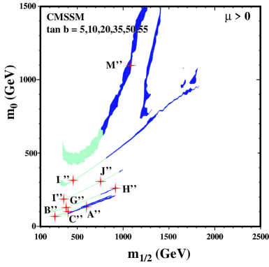
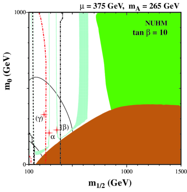
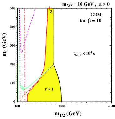
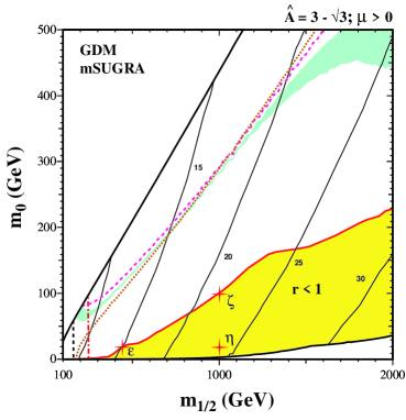
Figure 1: The allowed regions in the $(m_{1/2},m_{0})$ planes for (a) the CMSSM with a neutralino LSP [light/dark (blue) shaded strips], (b) the NUHM with a neutralino LSP for $\mu=375$ GeV and $m_{A}=265$ GeV [light (blue) shaded strips], (c) the CMSSM with a gravitino LSP weighing 10 GeV, and (d) mSUGRA with a gravitino LSP [light (yellow) shaded regions labelled $r<1$], for $A\equiv{\hat{A}}m_{0}:{\hat{A}}=3-\sqrt{3}$. In each case, the proposed benchmark scenarios are indicated by (red) crosses. Panel (a) displays WMAP strips for $\tan\beta=5,10,20,35,50,55$, panels (b, c) have $\tan\beta=10$, and in panel (d) $\tan\beta$ is fixed by the electroweak vacuum conditions with the values indicated along the (solid black) contours.

As noted above, the latest version of SSARD has been used to calculate these WMAP strips. It has an improved treatment of higher-order corrections, which are significant at large $\tan\beta$ and particularly in the very sensitive rapid-annihilation funnel region, which is now barely visible for $\tan\beta=50$ and $m_{t}=172.7$ GeV, but present for $\tan\beta=55$, as seen in Fig. 1a. We have adjusted minimally the parameters of previous CMSSM benchmark points with $\mu>0$, so as to leave unchanged the previous collider phenomenology and keep the relic density $\Omega_{\chi}h^{2}$ within the WMAP range. The corresponding changes in (mainly) $m_{0}$ and (occasionally) $m_{1/2}$ and $\tan\beta$ are tabulated in Table 1 where we indicate the values of $m_{1/2}$ and $m_{0}$ for the previous (single-primed) points [9]. Note that we have not updated the previous ‘focus-point’ benchmark scenarios (these are extremely sensitive to $m_{t}$, whose measurements at the Tevatron collider are still evolving significantly), nor the points with $\mu<0$ that are disfavoured by $g_{\mu}-2$.

Updated CMSSM benchmark scenarios
 
Model A^′′ B^′′ C^′′ G^′′ H^′′ I^′′ J^′′ L^′′ M^′′ $m_{1/2}$ 600 250 400 375 910 350 750 450 1075 (935) (1840) $m_{0}$ 135 65 95 125 260 180 300 310 1100 (120) (60) (85) (115) (245) (175) (285) (300) $\tan{\beta}$ 5 10 10 20 20 35 35 50 55 (50)

Table 1: We list updated GUT-scale input parameters for CMSSM benchmark scenarios with $\mu>0$ in the coannihilation and rapid-annihilation funnel regions. In scenarios where the values of $m_{1/2},m_{0}$ and/or $\tan\beta$ have been changed so as to keep $\Omega_{\chi}h^{2}$ within the WMAP range, as calculated with the latest version of SSARD, the previous input values are listed below in brackets. These points are valid for $m_{t}=172.7$ GeV.

For any given value of $m_{1/2}$ and $m_{0}$, the NUHM has two additional parameters, reflecting the degrees of non-universality $\delta_{u,d}$ of the masses of the two MSSM Higgs doublets [11]: $m_{H_{u,d}}^{2}=(1+\delta_{u,d})m_{0}^{2}$. One representative example of an NUHM plane is shown in panel (b) of Fig. 1, where we have assumed for definiteness that $\mu=375$ GeV and $m_{A}=265$ GeV, using $m_{t}=178$ GeV . The pale (turquoise) region allowed by cosmology includes a small ‘bulk’ region at low $m_{1/2}$ and $m_{0}$ that extends into a short coannihilation strip. There is then a near-vertical rapid-annihilation funnel whose location is determined by the choice of $m_{A}$, which is flanked by very narrow allowed WMAP strips at both larger and smaller values of $m_{1/2}$. There is then a continuation of the coannihilation strip and finally a third, broader vertical band where the relic density falls within the range allowed by WMAP. The latter band is a result of the fact that the LSP is becoming more Higgsino-like as $m_{1/2}>\mu$. The dark (brick) shaded region at large $m_{1/2}$ and small $m_{0}$ is forbidden because here the LSP would the (stable) ${\tilde{\tau}}_{1}$ and the medium (green) shaded region at large $m_{1/2}$ and $m_{0}$ is excluded by $b\to s\gamma$. Only regions between the two near-vertical black dot-dashed lines have effective potentials that are stable up to the GUT scale, and are hence permissible theoretically. The near-vertical black dashed and red dot-dashed lines represent the LEP constraints on $m_{\chi^{\pm}},m_{h}$ respectively . Thus, only the two narrow WMAP strips above the dark (brick) shaded region between the near-vertical red and black dot-dashed lines are consistent with all the constraints.

We see that one of the options opened up by the NUHM is a range of values of $m_{0}$ that are considerably larger than the very narrow range of values allowed by the CDM constraint in the CMSSM coannihilation strip, for any fixed values of $m_{1/2},\tan\beta$ and $A_{0}$. In the next Section, we exploit this freedom to increase $m_{0}$ by proposing three larger-$m_{0}$ scenarios shown as red crosses in the $(m_{1/2},m_{0})$ plane. One of these has the same values of $\mu,m_{A}$ as those chosen in panel (b) of Fig. 1, whereas the other two (indicated in brackets) have different values of $\mu,m_{A}$. As discussed in more detail below, the specific values of $\mu,m_{A},m_{1/2}$ and $m_{0}$ were chosen so as to offer various different sparticle cascade decay signatures including decays of the second-lightest neutralino $\chi_{2}\to h\chi,Z\chi$ that are not favoured in CMSSM scenarios with a neutralino LSP, as was discussed in [9].

Similar large values of $m_{0}$ are also attainable in the CMSSM, if the LSP is the gravitino. A representative sample $(m_{1/2},m_{0})$ plane in such a GDM scenario is shown in panel (c) of Fig. 1, where we made the particular choice $m_{3/2}=10$ GeV . The light (yellow) shaded region labelled by $r<1$ is that allowed not only by accelerator constraints (the LEP $m_{\chi^{\pm}}$ and $m_{h}$ limits are shown as near-vertical dashed black and dot-dashed red lines, respectively) but also by astrophysical and cosmological constraints [34]. Only below the diagonal dashed purple line can one satisfy the CDM constraint on the relic density of gravitinos produced in decays of the NLSP. However, the most stringent cosmological constraints in this GDM scenario come from comparing the baryon-to-entropy ratio inferred from measurements of the Cosmic Microwave Background (CMB) with that inferred from the measured Big-Bang Nucleosynthesis (BBN) calculations and light-element abundances, which might have been altered by NLSP decay products [34, 15] . The light elements whose abundances we include in this analysis are ⁴He, ³He, Deuterium, ⁶Li and ⁷Li. Also shown in panel (c) of Fig. 1 is the dotted line where $m_{\chi}=m_{{\tilde{\tau}}_{1}}$, above which the NLSP is the lightest neutralino $\chi$, and below which the NLSP is the lighter stau slepton ${{\tilde{\tau}}_{1}}$, which decays predominantly into $\tau$ gravitino. For comparison, the region with pale (turquoise) shading is the strip in the $(m_{1/2},m_{0})$ plane that would have been allowed if the lightest neutralino were the LSP.

The GDM benchmark point $\delta$ shown in panel (c) of Fig. 1 again has much larger $m_{0}$ and important $\chi_{2}\to h\chi,Z\chi$ decays. In this case, since the NLSP is the $\chi$ which has a lifetime $\sim 1.8\times 10^{4}$ s, it has no collider signature apart from missing transverse energy. This scenario therefore looks qualitatively similar to the CMSSM scenarios discussed earlier [7, 9], apart from its different and larger value of $m_{0}$.

In probing the possibilities for GDM with values of $m_{0}$ below the $m_{\chi}=m_{{\tilde{\tau}}_{1}}$ line in the $(m_{1/2},m_{0})$ plane, we propose below to study more restricted mSUGRA scenarios with $m_{3/2}=m_{0},A_{0}=(B_{0}+1)m_{0}$ and the Polonyi choice $A_{0}=(3-\sqrt{3})m_{0}$ [19], as seen in panel (d) of Fig. 1, which was produced using $m_{t}=178$ GeV . The dashed, dot-dashed and dotted lines and the pale (turquoise) strip have the same significances as in panel (c). Also shown as solid lines are contours of $\tan\beta$, as fixed by the electroweak vacuum conditions. In the low-$m_{0}$ region, the NLSP is the ${\tilde{\tau}}_{1}$, and its lifetime within the light (yellow) shaded region varies between $\sim 3\times 10^{6}$ and $10^{4}$ s.

We propose to survey this wedge-shaped GDM region by studying the three indicated points $\epsilon,\zeta,\eta$ located at the vertex and along the top and bottom sides of the wedge. In all these benchmark scenarios, the metastable ${\tilde{\tau}}_{1}$ would be detectable as a charged particle with an anomalously long time of flight. As pointed out in [35, 36], one might hope to trap some of the slower-moving charged NLSPs and detect their decays. However, the strategies and prospects for detecting and trapping ${\tilde{\tau}}_{1}$’s would be rather different for NLSPs with lifetimes measured in hours or months, as we discuss later.

3 Proposed New Benchmark Scenarios

We now describe in more detail the proposed new benchmark scenarios. As shown in Fig. 1(a), previous benchmarks were located along the WMAP lines in the CMSSM parameter space where $0.094<\Omega_{\chi}h^{2}<0.129$, which are very narrow in $m_{0}$ for any fixed values of $m_{1/2},\tan\beta$ and $A_{0}$. As seen in Fig. 2, the orderings of sparticle masses vary in important ways across the CMSSM $(m_{1/2},m_{0})$ plane, with important implications for the allowed and dominant sparticle decay modes. However, within the CMSSM, points with larger $m_{0}$ generally have larger values of $\Omega_{\chi}h^{2}$, and hence are cosmologically unacceptable .

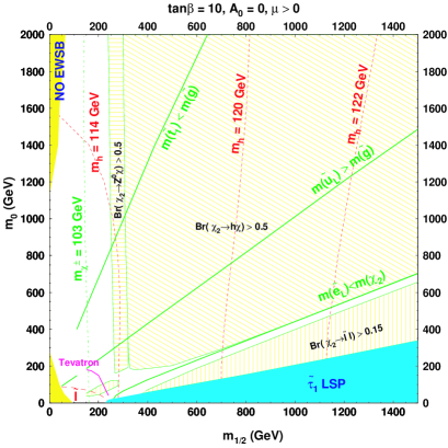
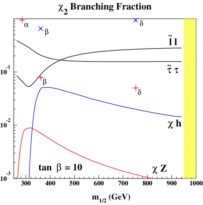
Figure 2: Left panel: Illustration of relevant aspects of the sparticle spectrum ordering and important decay modes in the $(m_{1/2},m_{0})$ plane of the CMSSM for $\tan\beta=10,\mu>0$ and $A_{0}=0$. Right panel: Decay modes of the second neutralino $\chi_{2}\to\chi Z$ (plus signs) and $\chi h$ (crosses) in various NUHM and GDM benchmark scenarios, compared with the corresponding branching ratios along the the WMAP line for $\tan\beta=10$ and $\mu>0$ discussed in [9]. These plots were obtained with PYTHIA 6.215 [37] interfaced to ISASUGRA 7.69 [21].

In particular, along the CMSSM WMAP strips and specifically in the previous benchmark scenarios, the branching ratios $\chi_{2}\to h\chi,Z\chi$ are generally quite small. The decays $\chi_{2}\to{\tilde{\ell}}\ell$ dominate in this region, as illustrated in both panels of Fig. 2. This is rather exceptional, since, as seen in the left panel, there is a large region of the CMSSM parameter space where $\chi_{2}\to\chi h$ decays dominate. These could play an important role in the discovery of the lightest Higgs boson $h$, as well as in reconstructing the sparticle cascade decays [26, 38]. There is also a band of low values of $m_{1/2}$ and relatively large values of $m_{0}$ where $\chi_{2}\to\chi Z$ decays are important, which does not happen along the WMAP strips, as seen in the right panel of Fig. 2. Even more strikingly, in models with values of $m_{0}$ significantly smaller than the WMAP strip value for any given choices of $m_{1/2},\tan\beta$ and $A_{0}$, the LSP would be the ${\tilde{\tau}}_{1}$, but such a charged LSP would be forbidden by astrophysics. However, scenarios with values of $m_{0}$ very different from those in the WMAP strips can be consistent with cosmology beyond the specific CMSSM framework considered in [7, 9], as we now discuss.

3.1 NUHM Benchmark Scenarios

When one considers models with non-universal soft supersymmetry-breaking contributions to the Higgs masses (NUHM), the electroweak vacuum conditions no longer fix $|\mu|$ and the pseudoscalar Higgs mass $m_{A}$ as they do in the CMSSM, so that both $m_{0}$ and the $\chi_{2}-\chi$ mass difference can be increased in such a way that the decays $\chi_{2}\to\chi h,Z$ are kinematically accessible but not competing decay modes into sleptons. We have chosen to exemplify the new phenomenology these decay modes open up by proposing consideration of three NUHM benchmark scenarios with relatively small sparticle masses that are beyond the reach of the Fermilab Tevatron collider, but would provide plenty of early physics opportunities for the LHC and substantial follow-up opportunities for the ILC .

As seen in Table 2 and as a (red) cross in Fig. 1(b), NUHM benchmark $\alpha$ has $\tan\beta=10$ and $m_{1/2}=285$ GeV, which is close to the value $m_{1/2}=250$ GeV in the CMSSM benchmark B^′′ (or SPS1a [8]). However, as seen in panel (b) of Fig. 1, it has a larger value of $m_{0}=210$ GeV, as compared to the CMSSM benchmark B^′′ value $m_{0}=65$ GeV. This ensures that $\chi_{2}\to{\tilde{\ell}}\ell$ decays are kinematically forbidden, as well as $\chi_{2}\to\chi h$, whereas $\chi_{2}\to\chi Z$ is possible and prominent, thanks to the mass difference $m_{\chi_{2}}-m_{\chi}=99$ GeV. As also seen in Table 2, this benchmark has $\mu=375$ GeV and $m_{A}=265$ GeV, as for the $(m_{1/2},m_{0})$ plane shown in panel (b) of Fig. 1. The choice of $m_{A}$ has the important consequence that rapid annihilation via the $A$ pole occurs at lower $m_{1/2}$, reducing the $\chi$ LSP density to the allowed cosmological range, as seen from the location of point $\alpha$ on one of the thin WMAP strips in panel (b) of Fig. 1 . We also note the degrees of non-universality in the soft supersymmetry-breaking Higgs masses:

$$m^{2}_{H_{u}}=-(333{\rm GeV})^{2},\;m^{2}_{H_{d}}=+(294{\rm GeV})^{2},$$ (3)

where $H_{u}$ ($H_{d}$) give masses to the $u$-type quarks ($d$-type quarks and charged leptons), respectively. These correspond to violations of Higgs universality that are ${\cal O}(1)$ . Coincidentally, the value of $m_{1/2}$ at the benchmark point $\alpha$ is close to the value of $m_{1/2}$ at the $\tan\beta=10$ CMSSM point that minimized $\chi^{2}$ in a fit to accelerator data including $m_{W},\sin^{2}\theta_{W},b\to s\gamma$ and $g_{\mu}-2$ [25]. The value of $\chi^{2}$ is not very sensitive to $m_{0}$, so its value at benchmark $\alpha$ is not very different from the minimum value in the CMSSM, as seen in Table 3. This Table also lists this point’s values of $\Omega_{\chi}h^{2},b\to s\gamma$ and the supersymmetric contribution to $g_{\mu}-$2.

Supersymmetric spectra in NUHM and GDM benchmark scenarios
 
Model $\alpha$ $\beta$ $\gamma$ $\delta$ $\epsilon$ $\zeta$ $\eta$ $m_{1/2}$ 285 360 240 750 440 1000 1000 $m_{0}$ 210 230 330 500 20 100 20 $\tan{\beta}$ 10 10 20 10 15 21.5 23.7 sign($\mu$) $+$ $+$ $+$ $+$ $+$ $+$ $+$ $A_{0}$ 0 0 0 0 25 127 25 $m_{t}$ 178 178 178 178 178 178 178 Masses $|\mu|$ 375 500 325 927 578 1176 1161 h⁰ 115 117 114 122 119 124 124 H⁰ 266 325 240 1177 641 1307 1277 A⁰ 265 325 240 1177 641 1307 1277 H^± 277 335 253 1180 646 1310 1279 $\chi^{0}_{1}$ 113 146 95 323 183 436 436 $\chi^{0}_{2}$ 212 279 178 625 349 840 840 $\chi^{0}_{3}$ 388 515 341 954 578 1176 1165 $\chi^{0}_{4}$ 406 528 358 964 593 1186 1175 $\chi^{\pm}_{1}$ 212 279 177 625 349 840 840 $\chi^{\pm}_{2}$ 408 529 360 965 594 1186 1176 $\tilde{g}$ 674 835 575 1610 986 2097 2097 $e_{L}$, $\mu_{L}$ 296 346 376 702 298 664 657 $e_{R}$, $\mu_{R}$ 216 241 328 571 169 383 370 $\nu_{e}$, $\nu_{\mu}$ 285 337 367 697 287 660 652 $\tau_{1}$ 212 239 315 564 150 340 322 $\tau_{2}$ 298 348 377 700 302 661 655 $\nu_{\tau}$ 285 337 364 695 285 651 644 $u_{L}$, $c_{L}$ 648 793 612 1532 897 1892 1889 $u_{R}$, $c_{R}$ 637 778 607 1480 867 1817 1814 $d_{L}$, $s_{L}$ 653 797 617 1534 901 1893 1891 $d_{R}$, $s_{R}$ 630 768 599 1474 864 1807 1805 $t_{1}$ 471 596 434 1159 682 1465 1472 $t_{2}$ 652 784 600 1429 879 1758 1756 $b_{1}$ 590 727 540 1395 824 1726 1723 $b_{2}$ 629 767 594 1468 862 1781 1775

Table 2: Proposed NUHM ($\alpha,\beta,\gamma$) and GDM ($\delta,\epsilon,\zeta,\eta$) benchmark points and mass spectra (in GeV), as calculated using SSARD [20] and FeynHiggs [39], using the one-loop corrected effective potential computed at the electroweak scale and one-loop corrections to the chargino and neutralino masses. We use here $m_{b}(m_{b})^{\overline{MS}}=4.25$ GeV and $m_{t}=178$ GeV.

Relic density $\Omega_{\chi}h^{2},b\to s\gamma$ and $g_{\mu}-2$ in post-WMAP benchmark scenarios, also $\tau_{NLSP}$ in the GDM models
 
$\alpha$ $\beta$ $\gamma$ $\delta$ $\epsilon$ $\zeta$ $\eta$ $\Omega_{LSP}h^{2}$ 0.12 0.10 0.09 0.07 $0.9\times 10^{-3}$ $0.9\times 10^{-2}$ $1.6\times 10^{-3}$ $\delta a_{\mu}$($10^{-9}$) 1.5 1.0 2.6 0.2 1.8 0.5 0.5 $B_{s\gamma}$($10^{-4}$) 4.1 4.4 2.8 3.7 3.6 3.6 3.6 $\tau_{NLSP}$(s) $---$ $---$ $---$ $1.8\times 10^{4}$ $3.3\times 10^{6}$ $2.0\times 10^{6}$ $6.8\times 10^{4}$ $\chi^{2}$ 1.93 3.67 1.98 6.81 1.15 6.25 5.99

Table 3: Comparison of $\Omega_{LSP}h^{2}$ for the benchmark points in Table 2, as computed with the SSARD code [20], $\delta a_{\mu}$($10^{-9}$), the branching ratio for $b\to s\gamma$, the NLSP lifetime for GDM scenarios and the $\chi^{2}$ for a global fit to precision observables [25].

As also seen in Table 2 and as a bracketed (red) cross in Fig. 1(b), NUHM benchmark $\beta$ has $\tan\beta=10$ but the somewhat higher value of $m_{1/2}=360$ GeV and $m_{0}=230$ GeV. However, it has $\mu=500$ GeV and $m_{A}=325$ GeV, for which choices the $(m_{1/2},m_{0})$ plane would look somewhat different. As for point $\alpha$, the choice of $m_{A}$ ensures a suitable relic density via rapid annihilation. The non-universal soft supersymmetry-breaking Higgs masses-squared are:

$$m^{2}_{H_{u}}=-(461{\rm GeV})^{2},\;m^{2}_{H_{d}}=+(229{\rm GeV})^{2}.$$ (4)

These again correspond to violations of Higgs universality that are ${\cal O}(1)$. With the larger value of $\mu$ as compared to point $\alpha$, the $\chi_{2}-\chi$ mass difference is increased to 133 GeV, thereby opening up the decay mode $\chi_{2}\to\chi h$ ($m_{h}=117$ GeV at this point). Benchmark $\beta$ lies somewhat further from the CMSSM point with minimum $\chi^{2}$, but its overall value of $\chi^{2}$ is still acceptable, as seen in Table 3, along with its values of $\Omega_{\chi}h^{2},b\to s\gamma$ and $g_{\mu}-2$.

As also seen in Table 2, the final NUHM benchmark $\gamma$ has $\tan\beta=20$ and, as seen as a bracketed (red) cross in Fig. 1(b), the somewhat lower value of $m_{1/2}=240$ GeV, and the somewhat larger value of $m_{0}=330$ GeV. It also has $\mu=325$ GeV and $m_{A}=240$ GeV. The latter choice ensures an acceptable relic density, although with different values of $\mu$ and $m_{A}$ from those used in the rest of panel (b) of Fig. 1. The non-universal soft supersymmetry-breaking Higgs masses-squared are:

$$m^{2}_{H_{u}}=-(242{\rm GeV})^{2},\;m^{2}_{H_{d}}=+(373{\rm GeV})^{2}.$$ (5)

These also correspond to violations of Higgs universality that are ${\cal O}(1)$, not orders of magnitude. With the choices of $\tan\beta,m_{1/2}$ and $\mu$, the $\chi_{2}-\chi$ mass difference is decreased to 83 GeV, closing off the $\chi_{2}\to\chi Z,h$ decay modes. Moreover, with this large value of $m_{0}$, the sleptons are far from the kinematic range for $\chi_{2}$ decays, which are therefore dominated by non-specific three-body decays mediated mainly by virtual $Z$ exchange. As seen in Table 3, the overall $\chi^{2}$ is again quite small for this point, which has a value of $m_{1/2}$ rather similar to CMSSM benchmark B^′′ .

3.2 GDM Benchmark Scenarios

As discussed in the Introduction, one may construct GDM scenarios with values of $m_{0}$ that are either much larger or much smaller than that in the CMSSM for the same values of $\tan\beta,m_{1/2}$ and $A_{0}$.

GDM benchmark $\delta$ described in Table 2 has been chosen to exemplify phenomenology at a significantly larger value of $m_{0}$, specifically 500 GeV, as well as a moderately large value of $m_{1/2}=750$ GeV. Thus, it samples the ‘panhandle’ reaching to large $m_{0}$, as shown by the (red) cross in Fig. 1(c). The $\chi_{2}-\chi$ mass difference increases to 302 GeV in this scenario, and all the sparticles are significantly heavier than in the previous NUHM benchmarks. We recall that the NLSP in this scenario is the lightest neutralino $\chi$. However, the neutralino lifetime for decays into a gravitino is $1.8\times 10^{4}$ s, too long to be detectable in the neighbourhood of a plausible collider experiment. Because of its larger values of $m_{1/2}$ and $m_{0}$, in particular, the overall $\chi^{2}$ for this model is somewhat further from the global minimum, but it cannot be excluded on this ground.

Here and in the following GDM models, we obtain a contribution to the LSP relic density by first calculating the NLSP abundance following thermalization, annihilation and freeze-out, and then reducing the density by a factor $m_{3/2}/m_{NLSP}$ to allow for the subsequent NLSP decays to the gravitino LSP. We see from Table 3 that this contribution to the relic gravitino density lies below the preferred WMAP range, and this feature is even more marked for the other GDM models discussed below. The total cold dark matter could be raised into the WMAP range either by another gravitino production mechanism, such as thermal production in the very early Universe [13], or if there is another component in the cold dark matter, such as an axion or superheavy relic.

Benchmark scenario $\delta$ is just one point in a three-dimensional space parametrized by $(m_{1/2},m_{0},m_{3/2})$ for the specific choices $A_{0}=0$ and $\tan\beta=10$, which certainly includes regions that would be more accessible in the early days of the LHC or at the ILC. On the other hand, the high-$m_{0}$ panhandle extends to larger values of $m_{0}$ that are not shown. This region presumably also extends to larger values of $m_{1/2}$ than those shaded in Fig. 1, but these would have lower NLSP lifetimes, in which cases hadronic NLSP decays would also have to be taken into account when evaluating the astrophysical and cosmological constraints [34]. We do not explore these options, since the challenging nature of benchmark scenario $\delta$ already serves as an adequate counterweight to the ‘easy’ scenarios $\alpha,\beta$ and $\gamma$ with their relatively low values of $m_{1/2}$ and $m_{0}$.

Since benchmark point $\delta$ is CMSSM-like, changing $m_{t}$ to 172.7 GeV would produce very little change in the sfermion spectrum, the biggest effect being 1.5 % in $m_{\tilde{t}}$. The Higgs mass would drop by 4 GeV, $m_{A}$ would drop by 3 %, and $|\mu|$ would drop by 5 %. The latter two changes would also affect the heavy Higgses and heavy neutralinos and charginos by approximately 5 %.

In order to reduce the dimensionality of the parameter space to be explored by the remaining GDM benchmark scenarios, we next assume an mSUGRA framework in which $m_{3/2}=m_{0}$ and $A_{0}=B_{0}+m_{0}$. We further assume that $A_{0}=(3-\sqrt{3})m_{0}$ [19]. In this case, the value of $\tan\beta$ is fixed by the electroweak vacuum conditions and varies across the $(m_{1/2},m_{0})$ plane, as seen in panel (d) of Fig. 1. In addition to a (pale blue) WMAP strip with $\chi$ LSP at $m_{1/2}<1$ TeV, we also see a (yellow) GDM region of parameter space allowed by the astrophysical and cosmological constraints. It takes the form of a wedge that broadens as $m_{1/2}$ increases, throughout which the NLSP is the ${\tilde{\tau}}_{1}$. We choose as our next GDM benchmark $\epsilon$ the point shown as a (red) cross that is close to the vertex of this wedge, with $m_{1/2}=440$ GeV and $m_{0}=20$ GeV. In this case, $\tan\beta=15$, the ${\tilde{\tau}}_{1}$ NLSP has a mass of 150 GeV and a lifetime of $3.3\times 10^{6}$ s. At this point, the global $\chi^{2}$ is not far from the best fit in the CMSSM, as seen in Table 2.

As seen by two more (red) crosses in panel (d) of Fig. 1(d), we complement this LHC- and ILC-friendly point with two points that are more challenging. A priori, values of $m_{1/2}$ considerably beyond 2 TeV would be possible in this wedge: they would be beyond the reach of either the LHC or the ILC, although the CLIC reach in ${\tilde{\tau}}_{1}$ pair production would extend beyond $m_{1/2}=4$ TeV. We consider two points with $m_{1/2}=1$ TeV, which are already quite challenging for the LHC. The upper edge of the wedge is defined by the astrophysical and cosmological constraint on ${\tilde{\tau}}_{1}$ decays, and corresponds to a ${\tilde{\tau}}_{1}$ lifetime $\sim 3.3\times 10^{6}$ s. The lower edge of the wedge that we consider corresponds to a lifetime of $10^{4}$ s. Benchmark point $\zeta$ is close to the upper edge, with $m_{0}=100$ GeV and $\tan\beta\simeq 21.5$. Here the ${\tilde{\tau}}_{1}$ NLSP has a mass of 340 GeV and a lifetime of $2\times 10^{6}$ s. Benchmark point $\eta$ is close to the lower edge, with $m_{0}=20$ GeV and $\tan\beta=23.7$. Here the ${\tilde{\tau}}_{1}$ NLSP has a mass of 322 GeV and a lifetime of $6.8\times 10^{4}$ s. Both these points have rather larger values of $\chi^{2}$ than the best fit in the CMSSM, as also seen in Table 2, but these points cannot be excluded on these grounds.

The changes in the spectra due to the shift in $m_{t}$ would be as follows: $\tan\beta$ would be increased by $\sim 4$, $|\mu|$ would be lowered by 4 % and $m_{A}$ would be lowered by 5-7 %, with corresponding changes in the heavy Higgses, neutralinos and charginos. The light Higgs mass would be lowered by 3-4 GeV, and changes in the sfermion masses would typically be less than 1 %, with the exception of the lighter stau, whose mass would drop by about 7 %.

3.3 Discussion of Spectra

As in our previous papers on CMSSM benchmarks [7, 9], the parameters of the NUHM and GDM benchmarks were first specified using the code SSARD [20]. In order to facilitate the interfaces with standard simulation packages, the spectra calculated with SSARD were then matched using parameters of the ISASUGRA 7.69 code [21] to reproduce the main features of the SSARD spectra. The values of $m_{0}$ and $m_{1/2}$ were adjusted to give the same masses for the lightest neutralino $\chi$ and the lighter stau $\tilde{\tau}_{1}$. Then the Higgs mass parameters $m_{H_{u}}$ and $m_{H_{d}}$ were varied to reproduce the SSARD values of $m_{A}$ and $\mu$. As these choices altered slightly the values of $m_{\chi}$ and $m_{{\tilde{\tau}}_{1}}$, the procedure was then iterated. The final ISASUGRA 7.69 parameters are listed in Table 4. This procedure was not followed for the GDM points, as our results are less sensitive to the exact spectra, and here the SSARD inputs were used. Note the difference in the sign convention for $A_{0}$ between the two codes.

Supersymmetric spectra in NUHM and GDM benchmarks
calculated with ISASUGRA 7.69
 
Model $\alpha$ $\beta$ $\gamma$ $\delta$ $\epsilon$ $\zeta$ $\eta$ $m_{1/2}$ 293 370 247 750 440 1000 1000 $m_{0}$ 206 225 328 500 20 100 20 $\tan{\beta}$ 10 10 20 10 15 21.5 23.7 sign($\mu$) $+$ $+$ $+$ $+$ $+$ $+$ $+$ $A_{0}$ 0 0 0 0 -25 -127 -25 $m_{t}$ 178 178 178 178 178 178 178 Masses $|\mu|$ 375 500 325 920 569 1186 1171 h⁰ 115 117 115 122 119 124 124 H⁰ 267 328 241 1159 626 1293 1261 A⁰ 265 325 240 1152 622 1285 1253 H^± 278 337 255 1162 632 1296 1264 $\chi^{0}_{1}$ 113 146 95 310 175 417 417 $\chi^{0}_{2}$ 215 282 180 600 339 805 804 $\chi^{0}_{3}$ 380 503 332 925 574 1192 1176 $\chi^{0}_{4}$ 400 518 352 935 587 1200 1184 $\chi^{\pm}_{1}$ 215 283 180 601 340 807 806 $\chi^{\pm}_{2}$ 399 518 352 935 587 1200 1184 $\tilde{g}$ 711 880 619 1691 1026 2191 2191 $e_{L}$, $\mu_{L}$ 299 351 378 713 306 684 677 $e_{R}$, $\mu_{R}$ 216 241 328 572 171 387 374 $\nu_{e}$, $\nu_{\mu}$ 287 340 368 703 290 669 662 $\tau_{1}$ 213 239 315 565 153 338 319 $\tau_{2}$ 300 352 378 712 309 677 670 $\nu_{\tau}$ 287 340 365 700 288 660 653 $u_{L}$, $c_{L}$ 674 826 636 1604 935 1991 1998 $u_{R}$, $c_{R}$ 661 808 629 1550 902 1911 1908 $d_{L}$, $s_{L}$ 679 831 642 1606 938 1993 1990 $d_{R}$, $s_{R}$ 652 797 621 1544 899 1903 1900 $t_{1}$ 492 622 453 1219 710 1545 1553 $t_{2}$ 662 800 611 1486 900 1842 1840 $b_{1}$ 609 752 558 1456 852 1807 1804 $b_{2}$ 641 785 603 1516 883 1851 1846

Table 4: Proposed NUHM and GDM benchmark points and mass spectra (in GeV), as calculated using ISASUGRA 7.69 [21] and adapting the input parameters to give the best match to the SSARD [20] spectra shown in Table 2, as described in the text.

As already mentioned, the first three of the new benchmarks, $\alpha,\beta,\gamma$, are NUHM points chosen to yield rather low-mass spectra, observable at an early stage of the LHC running, as might also point $\epsilon$. They also offer interesting physics opportunities for the ILC. These points complement the previous benchmark points B^′, C^′ and I^′ of [7, 9], as they give rise to different search topologies. On the other hand, points $\delta,\zeta$ and $\eta$ have heavier sparticles, and hence are much more challenging for both the LHC and the ILC.

4 Sparticle Decay Branching Ratios

One of the key particles appearing in sparticle decay chains is the second neutralino $\chi_{2}$, whose branching ratios are quite model-dependent and have significant impact on sparticle detectability at future colliders [6, 7, 8, 9, 26, 27]. In particular, $\chi_{2}$ decays play crucial roles in reconstructing the masses of heavier sparticles such as squarks and gluinos via cascade decays. Moreover, $\chi_{2}$ decays may offer new ways to discover or measure other new particles, such as the lightest MSSM Higgs boson $h$. Therefore, we now use ISASUGRA 7.69 to discuss the principal branching ratios of the $\chi_{2}$ in the various NUHM and GDM benchmark scenarios introduced above, comparing them in particular with those in the CMSSM at different points along the WMAP line for $\tan\beta=10$ and $\mu>0$, as discussed in [9].

We first recall the principal branching ratios of the $\chi_{2}$ in the low-mass CMSSM benchmarks considered previously. In the case of point B^′, the dominant decay mode was $\chi_{2}\rightarrow\tilde{\ell}_{R}\ell$ (11 %) followed by $\tilde{\ell}_{R}\rightarrow\chi\ell$, whereas in the case of point C^′ the dominant decay mode was $\chi_{2}\rightarrow\tilde{\ell}_{L}\ell$ (11 %) followed by $\tilde{\ell}_{L}\rightarrow\chi\ell$. On the other hand, in the case of point I^′, which has a relatively large value of $\tan\beta=35$, the dominant decay was $\chi_{2}\rightarrow{\tilde{\tau}}_{1}\tau$ (96 %), followed by ${\tilde{\tau}}_{1}\rightarrow\chi\tau$.

The new points $\alpha,\beta,\gamma$ provide qualitatively new signatures, as shown in Fig. 2. At the point $\alpha$, the $\chi_{2}$ mainly decays via $\chi_{2}\rightarrow Z\chi$ (96 %), which is observable through the $Z$ leptonic decay mode. At the point $\beta$, the main decay signature is $\chi_{2}\rightarrow h\chi$ (64 %), where the Higgs boson can be reconstructed from its decay to $\bar{b}b$. In addition, there are smaller branching ratios for $\chi_{2}\rightarrow Z\chi$ (8 %) and $\chi_{2}\rightarrow{\tilde{\tau}}_{1}\tau$ (23 %). On the other hand, point $\gamma$, which is just above the Higgs mass limit from LEP, has direct three-body leptonic decays $\chi_{2}\rightarrow\ell\bar{\ell}\chi$ (4 %) and $\chi_{2}\rightarrow\tau\bar{\tau}\chi$ (3 %), and the other decays are mainly $\chi_{2}\rightarrow q{\bar{q}}\chi$ mediated by virtual $Z$ exchange.

At all three points, the chargino decays dominantly into $W\chi$. At points $\alpha$ and $\beta$, the gluino is heavier than any of the squarks and decays to $\tilde{q}q$. The $\tilde{q}_{R}$ decays directly to $q\chi$, whereas the $\tilde{q}_{L}$ leads to cascade decays such as $\tilde{q}_{L}\rightarrow q\chi_{2}$ (typically $\sim$ 30 %) and $\tilde{q}_{L}\rightarrow q^{\prime}\chi^{\pm}$ (typically $\sim$ 60 %). On the other hand, at point $\gamma$ the gluino is lighter than the squarks of the first two generations, and its dominant decay is $\tilde{g}\rightarrow b\tilde{b}_{1}$ (81 %), followed by $\tilde{b}_{1}\rightarrow b\chi_{2}$ (26 %), $\tilde{b}_{1}\rightarrow t\chi^{\pm}$ (36 %) or $\tilde{b}_{1}\rightarrow t\chi^{\pm}_{2}$ (26 %). The squarks of the first two generations decay similarly as at points $\alpha$ and $\beta$ and with similar branching ratios.

As already remarked, at point $\delta$ the NLSP is the neutralino, which looks stable from the point of view of a collider detector, and gives rise to the usual missing-energy signature. As seen in Fig. 2, a further signature is provided by $\chi_{2}\rightarrow h\chi$ (91 %), with a smaller branching ratio for $\chi_{2}\rightarrow Z\chi$ (5 %). At this point also, the gluino is heavier than any of the squarks, whose decays are similar to those at points $\alpha$ and $\beta$.

At the last three points $\epsilon,\zeta,\eta$ with a ${\tilde{\tau}}_{1}$ NLSP, the gluino is heavier than any squark and decays to $\tilde{q}q$ with some preference for $\tilde{t}_{1}t$ ($\sim$ 20 %). The most important products of the subsequent squark cascade decays are displayed in Table 5, which we now explain. It is a general feature of these models that ${\tilde{q}}_{R}\to q\chi$ with branching ratios $\simeq 100$ %. Then $\chi\to{\tilde{\tau}}_{1}\tau$ with large branching ratios of 92/75/69 % in models $\epsilon,\zeta,\eta$, respectively, with essentially all the other decays being $\chi\to{\tilde{\ell}}_{R}\ell$ followed by ${\tilde{\ell}}_{R}\to\ell{\tilde{\tau}}_{R}\tau$. As a result, the dominant ${\tilde{q}}_{R}$ final states are $q{\tilde{\tau}}_{1}\tau$, with somewhat smaller fractions of $q\ell\ell{\tilde{\tau}}_{1}\tau$. Analogously, in many cases ${\tilde{q}}_{L}\to q\chi_{2}$, with branching ratios of 32/33/33 % in models $\epsilon,\zeta,\eta$, respectively, the other decays mainly being ${\tilde{q}}_{L}\to q^{\prime}\chi^{\pm}$. Many of the subsequent $\chi_{2}$ decays are also to ${\tilde{\tau}}_{1}\tau$, or else ${\tilde{\ell}}_{R}\ell$ followed again by ${\tilde{\ell}}_{R}\to\ell{\tilde{\tau}}_{R}\tau$ . Thus, ${\tilde{q}}_{L}$ decays via $\chi_{2}$ populate the final states $q{\tilde{\tau}}_{1}\tau$, $q\ell\ell{\tilde{\tau}}_{1}\tau$ and $q\ell\ell\ell^{\prime}\ell^{\prime}{\tilde{\tau}}_{1}\tau$. On the other hand, ${\tilde{q}}_{L}\to q^{\prime}\chi^{\pm}$ decays mainly populate final states containing neutrinos that would be more difficult to reconstruct, with the possible exception of some $q^{\prime}\tau W{\tilde{\tau}}_{1}$ final states.

Final state	$\epsilon$	$\zeta$	$\eta$
via $\chi_{2}$
$\tilde{q}_{L}\rightarrow qll\tilde{\tau}_{1}\tau$	6 %	7 %	6 %
$\tilde{q}_{L}\rightarrow qlll^{\prime}l^{\prime}\tilde{\tau}_{1}\tau$	0.5 %	2.3 %	2.9 %
$\tilde{q}_{L}\rightarrow q(Z,h)\tilde{\tau}_{1}\tau$	1.3 %	4 %	4 %
$\tilde{q}_{L}\rightarrow q\tau\tau\tilde{\tau}_{1}\tau$	1.2 %	0.8 %	0.6 %
$\tilde{q}_{L}\rightarrow q\tau\tau ll\tilde{\tau}_{1}\tau$	0.1 %	0.3 %	0.3 %
$\tilde{q}_{L}\rightarrow q\tilde{\tau}_{1}\tau$	4 %	1.3 %	1.5 %
decays with $\nu$’s	18 %	17 %	17 %
via $\chi^{\pm}$
$\tilde{q}_{L}\rightarrow q^{\prime}W\tilde{\tau}_{1}\tau$	6 %	10 %	10 %
decays with $\nu$’s	57 %	56 %	54 %
via $\chi$
$\tilde{q}_{R}\rightarrow q\tilde{\tau}_{1}\tau$	92 %	75 %	69 %
$\tilde{q}_{R}\rightarrow qll\tilde{\tau}_{1}\tau$	8 %	25 %	31 %

Table 5: Final states for the benchmark points with Gravitino Dark Matter (GDM), as calculated with ISASUGRA 7.69 [21].

The general conclusion is that LHC final states in these GDM models with ${\tilde{\tau}}_{1}$ NLSPs contain a pair of $\tau$ leptons and quite possibly additional lepton pairs, as seen in Table 5. In the case of benchmark scenario $\epsilon$, $m_{\chi_{2}}-m_{{\tilde{\ell}}_{L}}\simeq 35$ GeV and $m_{\chi}-m_{{\tilde{\tau}}_{1}}\simeq 23$ GeV, so the efficiency for picking up the additional cascade decay leptons may be reduced at the LHC , but in benchmark scenarios $\zeta,\eta$ these mass differences exceed 100 GeV, and these cascade decay leptons should be readily detectable.

5 Observability at Different Accelerators

5.1 Detectability at the LHC

We now provide rough estimates of the numbers of different species of supersymmetric particles that may be detectable at the LHC in the various NUHM and GDM benchmark scenarios introduced above. We assume the production cross sections for squarks and gluinos at the LHC that are listed in Table 6. The physics objects shown in the figures below are obtained in the following way.

$\bullet$ Jets are reconstructed from particles generated by the PYTHIA [37] Monte Carlo, using an iterative cone algorithm with a cone size of 0.5 radians. In order to model a typical LHC detector acceptance, we require each jet to have a pseudorapidity $|\eta|<3.0$ and a transverse energy $E_{T}>20$ GeV. These jets include hadronic tau decays.

$\bullet$ The missing transverse energy is calculated from the transverse energies $E_{T}$ of the visible particles.

$\bullet$ Charged leptons $e,\mu$ are accepted if their transverse momenta $p_{T}>10$ GeV and their pseudorapidities $|\eta|<2.4$. Their momenta are smeared with a Gaussian error between 1 % and 10 %, depending on the momentum.

$\bullet$ We assume a 50 % efficiency for identifying $b$ jets, with mis-tagging rates of 15 % for charm jets and 5 % for light quarks and gluons.

$\bullet$ We assume a 50 % efficiency for identifying hadronic $\tau$ decays, with a 6 % mis-tagging rate for jets with $E_{T}<30$ GeV and a 1 % mis-tagging rate for jets with $E_{T}>30$ GeV [26].

More complete and solid results should be obtained from detailed experimental simulations.

Model	$\alpha$	$\beta$	$\gamma$	$\delta$	$\epsilon$	$\zeta$	$\eta$
$\sigma({\tilde{g}}{\tilde{g}})$	5.8	1.4	16	0.008	0.45	0.001	0.001
$\sigma({\tilde{q}}{\tilde{g}})$	16	4.9	29	0.062	2.0	0.008	0.008
$\sigma({\tilde{q}}{\bar{\tilde{q}}})$	4.3	1.4	5.6	0.017	0.65	0.003	0.003
$\sigma({\tilde{q}}{\tilde{q}})$	3.9	1.6	5.2	0.050	0.85	0.012	0.012
$\sigma_{tot}({\tilde{g}})$	27	7.7	62	0.078	2.9	0.010	0.010
$\sigma_{tot}({\tilde{q}})$	32	11	51	0.20	5.0	0.038	0.038
$\sigma({\tilde{t}}_{1})$	1.1	0.29	1.7	0.004	0.13	0.001	0.001
$\sigma({\tilde{t}}_{2})$	0.17	0.055	0.28	0.001	0.026	0.000	0.000

Table 6: Cross sections in pb for models with non-universal Higgs masses (NUHM) or Gravitino Dark Matter (GDM) calculated with PROSPINO [40] at NLO and with masses from SSARD. The squark cross section is computed for the first 5 flavours. The quantity $\sigma_{tot}$ is the inclusive sum over all production mechanisms of the gluino or squark, e.g., $\sigma_{tot}({\tilde{g}})=2\;\sigma({\tilde{g}}{\tilde{g}})\sigma({\tilde{q}}{\tilde{g}})$. Production of $\tilde{t}_{1}$ and $\tilde{t}_{2}$ are not included in the sums, but listed separately.

We start with the benchmark points $\alpha$ to $\delta$, adopting criteria similar to those used previously in discussions of CMSSM benchmark scenarios with a neutralino LSP [7, 9].

$\bullet$ Higgs bosons: We generally follow the ATLAS and CMS studies of the number of observable Higgs bosons as a function of $m_{A}$ and $\tan\beta$ [26, 27], bearing in mind that they have no significant ‘exotic’ decay modes into non-Standard Model particles. The lightest neutral Higgs boson $h$ is detectable at all four points, and the heavier neutral Higgs bosons $H,A$ would be observable in scenarios $\alpha$, $\beta$ and $\gamma$. In contrast, the charged Higgs bosons $H^{\pm}$ would be observable only at point $\gamma$ where $\tan\beta=20$ since, according to previous studies [26, 27], $H^{\pm}$ cannot be seen at the LHC when $\tan\beta=10$, for any studied values of the other MSSM parameters.

$\bullet$ Gauginos: The lightest neutralino $\chi$ is considered always to be observable via the cascade decays of observed supersymmetric particles . We consider the $\chi_{2}$ to be observable at the LHC if the product of its production cross section and the relevant decay branching ratio ($\chi h,Z$ or $\ell^{+}\ell^{-}$) is at least 0.01 pb, corresponding to 1000 events produced with 100 fb^-1 of integrated luminosity. Thanks to the rather large production cross sections in Table 6, the $\chi_{2}$ is observable at all four points in the cascade decays of squarks. On the other hand, as the lighter chargino $\chi^{\pm}$ decays with a branching ratio $>90$ % into $W\chi$, it will be difficult to detect in cascade decays, so the possibility we have considered is via direct production of $\chi_{2}\chi^{\pm}$, leading to tri-lepton final states. Previous studies have indicated that the $\chi^{\pm}$ would not be observable in this mode for $m_{1/2}>170$ GeV, as in all the benchmark scenarios $\alpha,\beta,\gamma,\delta$. On the other hand, we note that the associated $\chi_{2}\chi^{\pm}$ production cross sections at points $\alpha,\gamma$ are $\sim 2.5,5.1$ fb, respectively, so these points would be worth further study.

One of the motivations for specifying the parameters of scenarios $\beta$ and $\delta$ was to consider models with large branching ratios for the cascade decays $\chi_{2}\to\chi h$, which have been studied previously by both ATLAS and CMS. Fig. 3 shows the cascade $h\to{\bar{b}}b$ signals expected in scenarios $\beta$ and $\delta$. We select events with missing $E_{T}>150$ GeV and require the candidate $b$ jets to be separated by an ‘angle’ $\Delta R\equiv\sqrt{\Delta\eta^{2}+\Delta\phi^{2}}<2$. We have generated 5000 sample supersymmetric events in each scenario: these correspond to integrated luminosities of less than one fb^-1 for scenario $\beta$ and about 50 fb^-1 for scenario $\delta$. The solid lines are the signals and the dashed lines are the supersymmetric backgrounds in the two scenarios from events not containing Higgs bosons : the Standard Model backgrounds are much smaller. The $h$ is visible in $\chi_{2}$ decays in scenario $\beta$ (we recall that the event sample corresponds to a very small integrated luminosity in this case) and the signal is even clearer at point $\delta$. Previous, more detailed CMS and ATLAS studies of low-mass points similar to $\beta$ have also concluded that the $h$ should be observable in sparticle cascade decays, and a point very similar to $\beta$ is being studied thoroughly for the CMS physics TDR [38]. Our first examination of point $\delta$ is promising, but more detailed studies of such a high-mass point would also be useful.

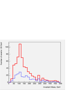
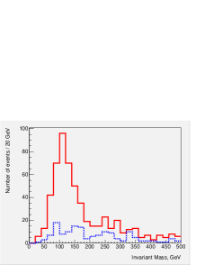
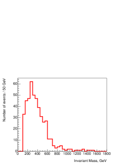
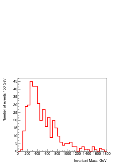
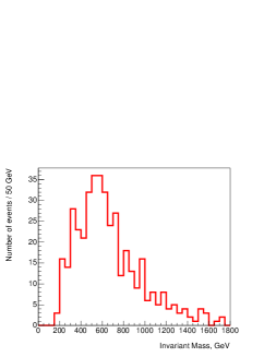
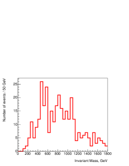
Figure 3: The signals from the lightest Higgs boson $h$ in $\chi_{2}\to\chi h$ cascade decays in scenarios (a) $\beta$ and (b) $\delta$, respectively, as found using PYTHIA [37] interfaced with ISASUGRA [21]. In each case, the solid line shows the sum of the supersymmetric signal and background, and the dashed line is the supersymmetric background alone. The Standard Model background is much smaller. The $qh$ invariant mass distributions in scenarios (c) $\beta$ and (d) $\delta$, respectively, each exhibit an end-point corresponding to ${\tilde{q}}_{R}\to q\chi_{2}$ cascade decays followed by $\chi_{2}\to\chi h$. The $qqh$ invariant mass distributions in scenarios (e) $\beta$ and (f) $\delta$, respectively, each exhibit a feature corresponding to ${\tilde{g}}\to{\tilde{q}}_{R}q$ and ${\tilde{q}}_{R}\to q\chi_{2}$ cascade decays followed by $\chi_{2}\to\chi h$.

$\bullet$ Squarks: The spartners of the lighter quark flavours $u,d,s,c$ are considered to be observable if $m_{\tilde{q}}<2.5$ TeV [41], so they could be observed in all four benchmark scenarios. However, their flavours could not be distinguished at the LHC. We further assume that the stops and sbottoms ${\tilde{t}},{\tilde{b}}$ are identifiable only if they weigh below 1 TeV, unless the gluino weighs $<2.5$ TeV and the stop or sbottom can be produced in its two-body decays. As in scenarios $\alpha,\beta,\gamma$ the stops and sbottoms are relatively light, we consider them to be observable. At point $\delta$, the branching ratio for ${\tilde{g}}\to{\tilde{t}}_{1}t\sim 40$ %, whereas the decays into ${\tilde{t}}_{2}t,{\tilde{b}}_{1}b$ and ${\tilde{b}}_{2}b$ are each only ${\cal O}(10)$ %. Accordingly, we consider only the $\tilde{t}_{1}$ to be detectable at point $\delta$. A note of caution is in order: since the detection of ${\tilde{t}}$ or ${\tilde{b}}$ production is difficult to assess without simulation studies, these conclusions should be taken with care.

We have considered the detectability of ${\tilde{q}}_{R}$ via their decays ${\tilde{q}}_{R}\to\chi_{2}q$ followed by $\chi_{2}\to\chi h$. Selecting the events in the $h$ peaks in $\chi_{2}$ decays shown in Fig. 3(a,b), and then combining the reconstructed $h$ boson with the hadronic jet ${J_{1}}$ that maximizes the product ${\mathbf{p}_{h}}\cdot{\mathbf{p}_{J_{1}}}$, we obtain the candidate $qh$ invariant mass distributions shown in panels (c, d) of Fig. 3 for points $\beta,\delta$, respectively. In principle, ${\tilde{q}}_{R}$ decays give end-points in these distributions, because of the two-body decay phase space, which are less distinctive than the corresponding dilepton edges in ${\tilde{q}}_{R}\to q\ell^{+}\ell^{-}\chi$ decays. Edge features are visible in both scenarios $\beta,\delta$, close to the expected positions at $\sim 600,1200$ GeV, respectively .

$\bullet$ Gluinos: These are generally considered to be observable for masses below 2.5 TeV [41], and hence can be discovered at all four points.

As seen in panels (e, f) of Fig. 3, we have also considered specific features of the searches for gluinos at points $\beta,\delta$, respectively. In each case, we have selected the hadronic jet ${J_{2}}$ that maximized the product ${\mathbf{p}_{J_{1}}}\cdot{\mathbf{p}_{J_{2}}}$ and plotted the $hJ_{1}J_{2}$ mass distribution. Gluino decays should give distinctive ‘edge’ features at $\sim 640,1280$ GeV, respectively, corresponding to the multi-body phase space. This feature is not very apparent for point $\beta$ with the small sample generated here, but more apparent for point $\delta$. A point similar to the former is also under study for the CMS Physics TDR [38]. A more detailed study of benchmark $\delta$ with optimized cuts would also be desirable.

We have also considered the decays ${\tilde{g}}\to{\tilde{b}}b$ at points $\alpha,\beta,\gamma$ and $\delta$. In each case, the product of the ${\tilde{g}}$ production cross section and branching ratio appears high enough to enable $m_{\tilde{g}}-m_{\tilde{b}}$ to be measured with sufficient accuracy to verify that this point has a value of $m_{0}$ significantly different from that on the CMSSM WMAP line for the same value of $m_{1/2}$. However, more refined studies of gluino search strategies would clearly be useful.

$\bullet$ Charged Sleptons: Since the mass differences $m_{\tilde{\ell}}-m_{\chi}\sim 100$ GeV at all these benchmarks, we consider ${\tilde{\ell}}$ decays into leptons always to be observable, provided that the slepton mass is light enough and hence the production cross section is large enough. We note that all four points have negligible branching ratios for the decays of $\chi_{2}$ to sleptons, which implies that cascades will not contribute to slepton observability and that sleptons can only be detected via their direct production. Following [7], we consider the direct production rates to be large enough if $m_{\tilde{\ell}}<350$ GeV. According to this criterion, all the charged sleptons would be observable in scenarios $\alpha$ and $\beta$ (though ${\tilde{\ell}}_{L}$ and ${\tilde{\tau}}_{2}$ signals would be very marginal at the latter point), and ${\tilde{e}}_{R},{\tilde{\mu}}_{R},{\tilde{\tau}}_{1}$ would be observable at point $\gamma$. However, we consider the observability of the $\tilde{\tau}_{1,2}$ to be difficult to assess without a detailed study and, conservatively, we do not count them as observable in any scenario. The sleptons are all too heavy to be observed at point $\delta$.

$\bullet$ Sneutrinos: We do not consider sneutrinos to be observable at the LHC. Although many of the sneutrino decays are into visible particles at points $\alpha,\beta,\gamma$, the modes $(\mu^{\pm}\chi^{\mp},\nu\chi_{2})$ having branching ratios (46, 20), (37, 17), (55, 33) % respectively. Moreover, the associated ${\tilde{\ell}}{\tilde{\nu}}$ production cross sections are quite large in scenarios $\alpha,\beta,\gamma$: 220/110/80 fb, respectively. Nevertheless, no viable discovery strategy has yet been developed.

We next discuss particle observabilities in the GDM scenarios $\epsilon,\zeta,\eta$, where $\tilde{\tau}_{1}$ is the NLSP. The branching ratios for final states resulting from the interesting cascade decays of squarks at the LHC are shown in Table 5. We first note that sparticle pair-production in these scenarios gives rise to substantial missing $E_{T}$, as seen in Fig. 4 for scenarios $\epsilon$ and $\zeta$ (point $\eta$ is very similar to the latter). We assume that the metastable ${\tilde{\tau}}_{1}$’s are measured in the detector, as discussed below. The missing $E_{T}$ is traceable to the many neutrinos in the final states, e.g., from $\tau$ decays and/or the many ${\tilde{q}}_{L}$ decays with other neutrinos.

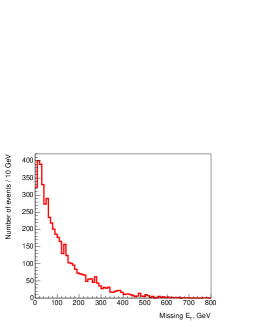
Figure 4: The missing $E_{T}$ spectra in scenarios $\epsilon$ and $\zeta$: that for point $\eta$ is similar to the latter. These plots were obtained with PYTHIA [37] interfaced with ISASUGRA [21].

We display in Figs. 5, 6 and 7 some other characteristics of events in these benchmark mSUGRA GDM scenarios. Panels (a) of Figs. 6 and 7 show the jet multiplicity distributions for points $\zeta,\eta$. Two-body decays of the ${\tilde{q}}_{R}$ are responsible for the bimodal distibutions of the leading jet transverse energies in panels (b) of both Figs. 6 and 7. The peak at $E_{T}\sim 1$ TeV is due to the two-body ${\tilde{q}}_{R}$ decays, and the lower-$E_{T}$ peak is due to other sparticle decays. Panels (c) of Figs. 6 and 7 show barely visible features in the leading lepton $E_{T}$ distributions due to slepton cascade decays. There is no such feature in Fig. 5, where the cascade lepton energy is smaller. Nevertheless, we note that large fractions of the cascade-decay leptons have transverse momenta large enough to be detected with high efficiency, and could potentially be used as event triggers in addition to the high-$E_{T}$ jets.

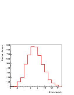
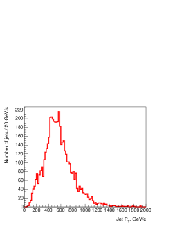
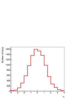
Figure 5: Kinematic distributions in events produced in the GDM benchmark scenario $\epsilon$: (a) hadron jet multiplicity, (b) the transverse energy $E_{T}$ of the most energetic jet, (c) the transverse energy $p_{T}$ of the most energetic lepton, and (d) the pseudorapidity distribution for ${\tilde{\tau}}_{1}$ production. These plots were obtained with PYTHIA [37] interfaced with ISASUGRA [21].

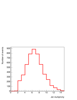
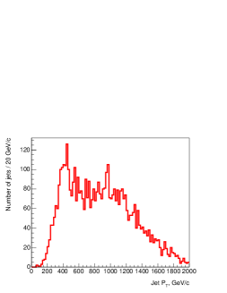
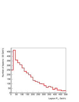
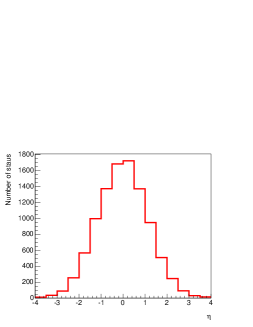
Figure 6: Kinematic distributions in events produced in the GDM benchmark scenario $\zeta$, as in Fig. 5.

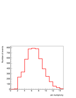
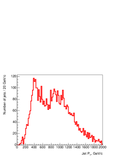
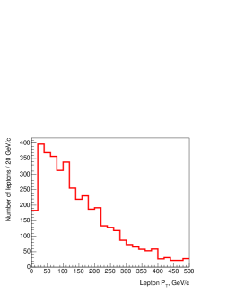
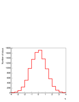
Figure 7: Kinematic distributions in events produced in the GDM benchmark scenario $\eta$, as in Fig. 5.

$\bullet$ Gravitino: We consider the gravitino to be observable in GDM scenarios where the NLSP can be stopped and its decays observed. This was obviously not the case in scenario $\delta$, considered above, and perhaps not in scenarios $\zeta,\eta$ either, as we discuss later. On the other hand (see below), it seems possible to obtain a substantial sample of $\tilde{\tau}_{1}$ decays in scenario $\epsilon$, so we consider the gravitino to be indirectly observable in this case.

$\bullet$ Sleptons: The ${\tilde{\tau}}_{1}$ has a distinctive time-of-flight signature, and we consider that it could be detected with some efficiency in both ATLAS and CMS in all the scenarios $\epsilon,\zeta,\eta$. As seen in panels (d) of Figs. 5, 6 and 7, it is generally produced quite centrally and in association with a considerable number of high-$E_{T}$ jets and/or leptons. As discussed below, its mass can probably be measured with an accuracy $\sim 1$ % in all three scenarios, and a significant sample of decays of stopped ${\tilde{\tau}}_{1}$’s should enable its lifetime to be measured at point $\epsilon$. Even in scenarios $\zeta,\eta$, one expects a sample of several hundred events with ${\bar{\tilde{q}}_{R}}{\tilde{q}}_{R}$ production followed by ${\tilde{q}}_{R}\to q(\chi\to{\tilde{\tau}}_{1}\tau)$ decay on one side, and ${\tilde{q}}_{R}\to q(\chi\to{\tilde{\ell}}_{R}\ell)$ decay on the other side, followed by ${\tilde{\ell}}_{R}\to\ell{\tilde{\tau}}_{1}\tau$ decay. We therefore expect the ${\tilde{\ell}}_{R}$ to also be observable at all three points. In scenario $\epsilon$, one should also be able to reconstruct the cascade ${\tilde{q}}_{L}\to q\chi_{2}$ followed by $\chi_{2}\to{\tilde{\ell}}_{L}\ell$ and then ${\tilde{\ell}}_{L}\to\chi\ell$. Knowing already the $\chi$ mass from the analysis of ${\tilde{q}}_{R}$ decays, one should be able to reconstruct the ${\tilde{\ell}}_{L}$ and $\chi_{2}$ masses at point $\epsilon$. At points $\zeta,\eta$, we expect a sample of a few dozen events, which might be sufficient to argue that $m_{{\tilde{\ell}}_{L}}>m_{\chi}>m_{{\tilde{\ell}}_{R}}>m_{{\tilde{\tau}}_{1}}$, and thereby provide some discrimination against GMSB models [43] , but would be insufficient to reconstruct the heavier slepton masses. In summary, therefore, we consider all the charged sleptons to be observable at point $\epsilon$, but only ${\tilde{\tau}}_{1}$ and ${\tilde{\ell}}_{R}$ at points $\zeta,\eta$.

$\bullet$ Sneutrinos: We do not consider these to be observable in any of the the three scenarios.

$\bullet$ Gauginos: The lightest neutralino $\chi$ should be observable in all three scenarios $\epsilon,\zeta,\eta$, as a resonance in ${\tilde{\tau}}_{1}\tau$ combinations, for example in ${\tilde{q}}_{R}\to q(\chi\to{\tilde{\tau}}_{1}\tau)$ cascade decays which have branching ratios of 92/75/69 % in the three scenarios. On the other hand, the second neutralino $\chi_{2}$ is probably observable only in ${\tilde{q}}_{L}$ decays, and only in scenario $\epsilon$. We do not consider the charginos and heavier neutralinos to be observable at any of these points.

$\bullet$ Higgs bosons: The $h$ should be observable in the three scenarios $\epsilon$ to $\eta$, but the heavier Higgs bosons are not expected to be observable in any of them.

$\bullet$ Squarks: At point $\epsilon$, all squark flavours, excluding the ${\tilde{t}}_{2}$ but including the ${\tilde{t}}_{1}$ and ${\tilde{b}}_{1,2}$ (which appear in 10/15/11 % of ${\tilde{g}}$ decays), should be observable. The spartners of the $u,d,s,c$ quarks could also be observed at points $\zeta,\eta$, but not the ${\tilde{t}}_{1,2}$ and ${\tilde{b}}_{1,2}$.

$\bullet$ Gluinos: According to our standard criteria, these should be observed in all three scenarios $\epsilon,\zeta,\eta$.

We have made a first examination of issues in the reconstruction of sparticle cascade decays in GDM benchmark scenarios $\epsilon,\zeta,\eta$, using as initial building-blocks the final-state ${\tilde{\tau}}_{1}$ and $\tau$. The $p_{T}$ distributions for hadronic $\tau$-decay jets at the three points are shown in Fig. 8(a, c, e), where we see that those at points $\zeta,\eta$ are significantly harder than at point $\epsilon$. The mis-tag probabilities we take from [26] are adequate for identifying the large-$p_{T}$ $\tau$ hadronic jets in GDM sparticle-pair-production events, which would have been collected by the normal large-$p_{T}$ trigger at the LHC. Using these tagging estimates, and combining the candidate $\tau$ hadronic jets with the ${\tilde{\tau}}_{1}$ tracks, which are assumed to be measured with an accuracy $\delta p/p=5$ %, we obtain the $\tau-{\tilde{\tau}}_{1}$ invariant-mass distributions shown in panels (b, d, f) of Fig. 8, respectively. In each case, we see a clear signal due to $\chi\to\tau{\tilde{\tau}}_{1}$ decays.

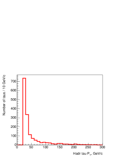
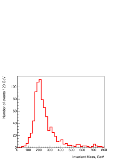
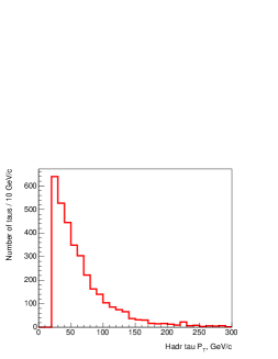
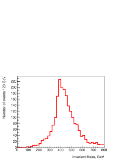
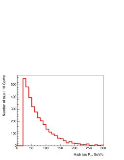
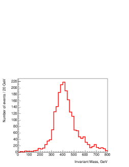
Figure 8: The $\tau$ $p_{T}$ distributions and the $\tau-{\tilde{\tau}}_{1}$ invariant-mass distributions for (a, b) benchmark scenario $\epsilon$, (c, d) benchmark scenario $\zeta$ and (e, f) benchmark scenario $\eta$.

We have then considered the reconstruction of higher cascade decays in scenarios $\epsilon$ and $\zeta$, the latter being very similar to point $\eta$. We find peaks in ${\tilde{\tau}}_{1}-\tau-\ell$ combinations corresponding to the ${\tilde{\ell}}_{L,R}$, and in ${\tilde{\tau}}_{1}-\tau-\ell-\ell$ combinations corresponding to the $\chi_{2}$. However, the combinatorial backgrouds have shapes quite similar to the signals. Full studies of these scenarios lie beyond the scope of this survey, but it does seem that sparticle cascades can be reconstructed in these scenarios, analogously to what was shown previously for scenarios with a $\chi$ LSP.

5.2 Detectability at $e^{+}e^{-}$ Linear Colliders

As in our previous studies [7, 9], our criteria for the observability of supersymmetric particles at linear colliders are based on their pair-production cross sections.

$\bullet$ Particles with cross sections in excess of 0.1 fb are considered as observable, because they would give rise to more than 100 events with an integrated luminosity of 1 ab^-1.

$\bullet$ The lightest neutralino $\chi$ is considered to be observable only through the decays of heavier supersymmetric particles.

$\bullet$ Sneutrinos are considered to be detectable when the sum of the branching fractions for decays which lead to clean experimental signatures, such as $\tilde{\nu}_{\ell}\to\chi^{\pm}\ell^{\mp}$ ($\ell$ = $e$, $\mu$, $\tau$) and $\tilde{\nu}_{\tau}\to W^{+}\tilde{\tau_{1}}^{-}$, exceeds 15 %.

$\bullet$ The $\gamma\gamma$ collider option at a linear collider would allow single production of heavy neutral Higgs bosons via the $s$-channel processes $\gamma\gamma\to A$ and $\gamma\gamma\to H$, extending the reach up to 375 GeV for 0.25 TeV $e^{\pm}$ beams, 750 GeV for 0.5 TeV $e^{\pm}$ beams, 2.0 TeV for 1.5 TeV $e^{\pm}$ beams and 3.75 TeV for 2.5 TeV $e^{\pm}$ beams. A $\gamma\gamma$ collider may also be used to look for gluinos [42], but we do not include this possibility in our analysis.

$\bullet$ Finally, we assume that a metastable ${\tilde{\tau}_{1}}$ could be detected at any linear $e^{+}e^{-}$ collider with more than 100 events, and note that the mass could be measured more accurately than at the LHC, by measuring the production threshold as well as $1/\beta$ (see the next Section for further discussion).

As previously [7, 9], we consider $e^{+}e^{-}$ collision energies $\sqrt{s}$ = 0.5 TeV, 1.0 TeV, 3 TeV and 5 TeV, and also the combined capabilities of the LHC and a 1-TeV linear collider.

$\bullet$ For $\sqrt{s}$ = 0.5 TeV, at NUHM benchmark point $\alpha$ the $\chi,\chi_{2},\chi_{1}^{\pm}$ and the lighter sleptons ${\tilde{\mu}}_{R},{\tilde{e}}_{R},{\tilde{\tau}}_{1}$ would be observable. The prospects at benchmark point $\beta$ are similar, except that the $\chi^{\pm}$ would not be observable. At benchmark point $\gamma$, all the inos except the $\chi_{2}^{\pm}$ would be observable, and the sleptons ${\tilde{\mu}}_{R},{\tilde{e}}_{R},{\tilde{\tau}}_{1}$ would be observable in $\chi_{4}$ decays. The lightest $h$ is always observable and the $H,A$ can be produced in $\gamma\gamma$ collisions for these benchmark points.

The prospects for the GDM benchmark points are not so good: apart from $h$, only ${\tilde{\mu}}_{R},{\tilde{e}}_{L,R},{\tilde{\tau}}_{1,2}$ are observable , and then only in the low-mass scenario $\epsilon$ that was chosen at the tip of the low-$m_{0}$ GDM wedge in mSUGRA parameter space. No squarks or gluinos are observable in any NUHM or GDM scenario at $\sqrt{s}$ = 0.5 TeV.

$\bullet$ For $\sqrt{s}$ = 1 TeV, all the neutralinos, charginos and sleptons (both charged and neutral) become observable in scenarios $\alpha,\beta$ and $\gamma$, and the heavy Higgs bosons can now be pair produced in $e^{+}e^{-}$ collisions directly. In the GDM scenario $\delta$, associated $\chi\chi_{2}$ production becomes observable, albeit with a low event rate, and ${\tilde{\mu}}_{R},{\tilde{e}}_{R},{\tilde{\tau}}_{1}$ production can be detected in $\chi_{2}$ decays. At point $\epsilon$, associated $\chi\chi_{2}$ production should again be observable, and probably also associated $\chi\chi_{3,4}$ production, as well as $\chi^{\pm}$ pair production, associated $\chi^{\pm}\chi_{2}^{\mp}$ production and pair-production of all the charged sleptons. Finally, at points $\zeta$ and $\eta$, only $\chi$, ${\tilde{\mu}}_{R},{\tilde{e}}_{R}$ and ${\tilde{\tau}}_{1}$ are expected to be observable.

$\bullet$ For $\sqrt{s}$ = 3 TeV, all the Higgs bosons, neutralinos, charginos, sleptons and squarks would be observable in each of the scenarios $\alpha,\beta,\gamma,\epsilon$. The same is true at benchmark point $\delta$, with the exception of the left-handed first- and second-generation squarks, and the right-handed squarks ${\tilde{t}}_{2}$ and ${\tilde{b}}_{2}$, because of their low rates. At benchmark points $\zeta,\eta$, one should observe all the weakly-interacting sparticles, but (with the exception of the ${\tilde{t}}_{1}$) the squarks would still be out of kinematic reach. At benchmark point $\gamma$, also the gluino will be observable in squark decays.

$\bullet$ For $\sqrt{s}$ = 5 TeV, the story is simple: all the sparticles except ${\tilde{g}}$ would be observable in all the proposed NUHM and GDM benchmarks, and also the ${\tilde{g}}$ at point $\gamma$.

5.3 Summary

Fig. 9 summarizes the numbers of different species of MSSM particles visible at different accelerators. We see that the LHC provides good coverage for strongly-interacting sparticles (uppermost green and pink bars) in all the NUHM and GDM benchmarks scenarios considered, whereas its coverage for weakly-interacting sparticles (middle red and blue bars) is rather uneven. The lightest Higgs boson is always detectable (lowest light blue bars) and in some cases also heavier Higgs bosons. In scenarios $\alpha,\beta,\gamma,\epsilon$, a linear $e^{+}e^{-}$ collider with $\sqrt{s}=0.5$ TeV would provide useful extra information about some weakly-interacting sparticles. In all cases, it would provide detailed measurements of one or more Higgs bosons. A linear $e^{+}e^{-}$ collider with $\sqrt{s}=1.0$ TeV would provide better information on both weakly-interacting sparticles and Higgs bosons, but still no information on squarks or gluinos. The combination of the LHC and a 1.0-TeV linear collider would provide good coverage overall, but this would still be incomplete in scenarios $\delta,\zeta,\eta$, in particular. A linear $e^{+}e^{-}$ collider such as CLIC with $\sqrt{s}=3.0$ TeV would provide detailed studies of all the weakly-interacting sparticles and Higgs bosons in all the scenarios studied, and also provide new opportunities to study squarks in scenarios $\alpha,\beta,\gamma,\delta,\epsilon$. Finally, CLIC at 5.0 TeV would provide detailed measurements of all the MSSM particles except possibly the gluino, for which one would still rely on the LHC .

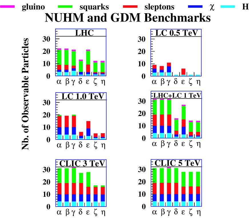
Figure 9: Summary of the numbers and types of MSSM particles that may be detected at various accelerators in the NUHM and GDM benchmark scenarios considered here. The gravitino may also be indirectly ‘observable’ at point $\epsilon$. We emphasize that these numbers are estimates that need to be validated by experimental simulations. As in [7, 9], we see that the capabilities of the LHC and of linear $e^{+}e^{-}$ colliders are largely complementary. We re-emphasize that mass and coupling measurements at $e^{+}e^{-}$ colliders are usually much cleaner and more precise than at the LHC, where, for example, it is not known how to distinguish the light squark flavours.

6 The Stau NLSP in GDM Scenarios

6.1 Production and Detectability at the LHC

In the mSUGRA GDM models studied here, all supersymmetric events yield a pair of ${\tilde{\tau}}_{1}$ NLSPs. The astrophysical BBN/CMB constraint prevents the ${\tilde{\tau}}_{1}$ lifetime from exceeding $\sim 3\times 10^{6}$ s [34], and we do not discuss here ${\tilde{\tau}}_{1}$ lifetimes smaller than $10^{4}$ s. Charged NLSPs with lifetimes in this range would appear to a generic collider detector like massive stable charged particles, and the three benchmark scenarios $\epsilon,\zeta,\eta$ studied here span this range of lifetimes.

Fig. 10 shows the distributions of the non-relativistic factor $\beta\gamma$ expected for the ${\tilde{\tau}}_{1}$’s in these mSUGRA GDM scenarios from cascade decays of squarks and gluinos at the LHC. The great majority of the ${\tilde{\tau}}_{1}$’s produced at the LHC are far from being ultra-relativistic, and so should yield exotic time-of-flight (TOF) and/or $dE/dx$ signals . The same would be true of ${\tilde{\tau}}_{1}$’s produced at the ILC, if its centre-of-mass energy reaches above the pair-production threshold in the corresponding scenarios, namely 310, 680 and 650 GeV in benchmarks $\epsilon,\zeta$ and $\eta$, respectively. CLIC with a centre-of-mass energy of 3 TeV would be able to produce ${\tilde{\tau}}_{1}$ pairs with masses $\leq 1.5$ TeV, and hence probe the GDM wedge out to $m_{1/2}\sim 4.5$ TeV.

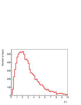
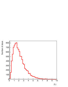
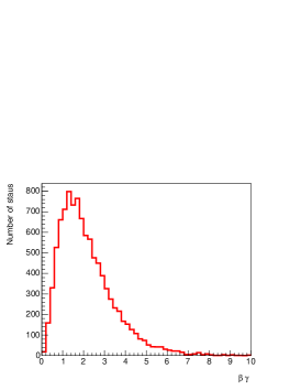
Figure 10: The spectra of the non-relativistic factor $\beta\gamma$ for the ${\tilde{\tau}}_{1}$’s produced at the LHC, in the benchmark scenarios $\alpha,\beta,\gamma$, respectively.

The key signal for GDM with a ${\tilde{\tau}}_{1}$ NLSP would in general be the coincident appearance in adjacent or nearby bunch crossings of generic high-$p_{T}$ triggers and subsequent ‘muon’ triggers. Such coincidences would be very rare for conventional trigger rates, which would give coincidence rates $<10^{-6}$ in adjacent bunch crossings.

The ${\tilde{\tau}}_{1}$ NLSP is often sufficiently non-relativistic, $\beta\gamma<1$, that it would not exit an LHC detector such as ATLAS or CMS before the next bunch crossing (25 ns after the event in which the ${\tilde{\tau}}_{1}$ was produced), in which case its tracking information might be lost. This issue could be addressed by reading out of the detector all the tracking signals that occurred within several crossing times following an ‘interesting’ event. ‘Interest’ would normally be defined by a conventional high-$p_{T}$ lepton or calorimetric trigger. As seen in Figs. 5, 6 and 7, most supersymmetric events would indeed pass the normal ATLAS and CMS criteria for ‘interesting’ events.

If a sample of interesting candidate events can be identified, one possible ${\tilde{\tau}}_{1}$ search strategy would be to select out of the usual high-$p_{T}$ lepton and calorimetric triggers a subsample of events suspected of containing ${\tilde{\tau}}_{1}$ NLSPs. Even if the muon systems do not trigger on the ${\tilde{\tau}}_{1}$’s, the muon drift tubes of both ATLAS and CMS integrate signals over a number of bunch crossings, such that hits of particles which are out of the normal 25-ns time window can still be recorded with the event. One would, however, need to adapt the track reconstruction software so as to allow for such signal time shifts and recuperate the full information. At the moment, in the absence of any good reason to take seriously such scenarios with massive, slow-moving charged particles, the only experimental strategy required from the ATLAS and CMS Collaborations is to avoid precluding the possibility of such a buffered readout, should it subsequently appear worthwhile for searches in GDM or other scenarios.

Alternatively, one could use the presence of a high-$p_{T}$ charged particle in the muon system as a primary trigger, and then look back through earlier bunch crossings for evidence of other high-$p_{T}$ jets and/or leptons, that would already have triggered the detector and been recorded.

6.2 Measuring the Stau Mass

A crude estimate of the obtainable $\tilde{\tau}_{1}$ mass resolution can be derived by propagating the uncertainties in the momentum measurement $\Delta p$ and in the TOF resolution $\Delta t$, as determined in a detector at a distance $L$:

$$\frac{\Delta M}{M}=\frac{\Delta p}{p}\bigoplus\beta\gamma^{2}\frac{\Delta t}{L}$$ (6)

For ATLAS and CMS, the expectations are $\Delta p/p\simeq 1-10$ % and $\Delta t\simeq$ 1 ns at a distance of $\sim 5$ m. Since the peak value of $\beta\gamma^{2}$, is $\sim 2$, as seen in Fig. 10, we estimate that in each event

$$\frac{\Delta M}{M}=(0.01-0.10)\bigoplus 0.12.$$ (7)

We therefore estimate that the $\tilde{\tau}_{1}$ mass could be measured with an error of 10 - 20 % in each event, which could be reduced by selecting low-momentum events as shown in Fig. 11, and further by combining measurements in many events. Panel (a) shows the distribution of the second term in (6) for $\tilde{\tau}_{1}$’s produced in a sample of events from benchmark point $\epsilon$, and panel (b) shows the distribution of the corresponding mass resolution $\Delta M$ obtainable event-by-event. Selecting now a sample of the 10 % of $\tilde{\tau}_{1}$’s with the lowest values of $\beta\gamma^{2}$, and hence, according to (6), those with the smallest values of $\Delta M$ , and assuming that $\Delta p/p$ has a Gaussian error of 5 %, we obtain panel (c) of Fig. 11. We see that almost all these individual events have $\Delta M/M<10$ %. The same is true for an anologous sample of events produced in a simulation of benchmark point $\zeta$, as seen in panel (d) of Fig. 11 and also for point $\eta$ (not shown). Therefore, if one could obtain a total sample of $\sim 1000$ $\tilde{\tau}_{1}$ events, and if systematic effects and correlations could be controlled, combining the best-measured 100 events could yield $\Delta M/M<1$ %.

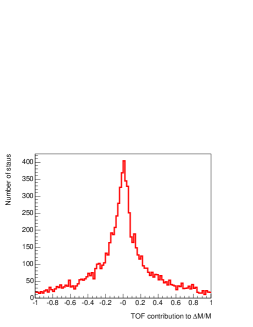
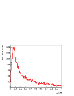
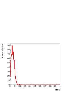
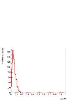
Figure 11: (a) The TOF contribution to the mass resolution $\Delta M/M$ (6) in the stau NLSP mass measurement, (b) the full uncertainty $\Delta M/M$ found for the complete event sample of benchmark point $\epsilon$, (c) $\Delta M/M$ for the 10 % of events at point $\epsilon$ with the lowest values of $\beta\gamma^{2}$, and (d) the same distribution for point $\zeta$ (the result for point $\eta$ is very similar).

To help assess the importance of such a measurement, we display in Fig. 12 how a 1 % ${\tilde{\tau}}_{1}$ mass measurement could be combined with a determination of the supersymmetric mass scale $m_{1/2}$ to determine the allowed range of parameters in the $(m_{1/2},m_{0})$ plane. If $m_{1/2}$ were known exactly, the error in $m_{{\tilde{\tau}}_{1}}$ would correspond to $\delta m_{0}\sim 20$ GeV, which should be compounded with the error induced by propagating the uncertainty in $m_{1/2}$. Such a determination of $m_{0}$ would enable a ballpark estimate of the ${\tilde{\tau}}_{1}$ NLSP lifetime to be made, within this mSUGRA GDM framework, enabling a strategy to search for its decays to be better focused, as also seen in Fig. 12.

The value of $m_{1/2}$ could perhaps be determined by measuring the gluino mass, but here we discuss the use of the total supersymmetric cross section. Comparing the total sparticle production cross section in scenario $\epsilon$ with those for scenarios $\zeta,\eta$, we see that $\sigma_{tot}\sim m_{1/2}^{-6}$, approximately. The statistical error in measuring $\sigma_{tot}$ for either of the scenarios $\zeta,\eta$ would be about 1.5 %, but we expect that the systematic and theoretical errors would be larger. Neglecting theoretical errors, an experimental error of 5 % would enable $m_{1/2}$ to be estimated with an uncertainty $<1$ % from the total cross section alone: see the vertical shaded band in Fig. 12 . Assuming also a measurement uncertainty of $\sim 1$ % in $m_{{\tilde{\tau}}_{1}}$, we see from Table 2 and Fig. 12 (diagonal shaded bands) that this should be sufficient to distinguish between scenarios $\zeta,\eta$ at the 5-$\sigma$ level. However, this discrimination would be lost if the error in either $m_{{\tilde{\tau}}_{1}}$ or $m_{1/2}$ rose to $\sim 5$ %.

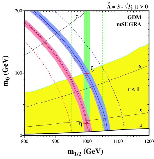
Figure 12: The potential impacts of prospective measurement errors of 1 % and 5 % for $m_{{\tilde{\tau}}_{1}}$ (diagonal bands and lines) and $m_{1/2}$ (vertical bands and lines) as constraints in the $(m_{1/2},m_{0})$ plane for GDM models in the mSUGRA framework. The smaller errors would enable the benchmark scenarios $\zeta$ and $\eta$ to be distinguished, and the possible NLSP lifetime to be estimated. The thin solid lines are labeled by the logarithm of the NLSP lifetime in seconds.

One could in principle also look for slowly-moving massive charged particles via an anomalous $dE/dx$ signal, for instance using high-threshold signals in the ATLAS TRT detector, and maybe using the electromagnetic calorimeter of either experiment . A good $dE/dx$ measurement is a design feature that could be considered for the central trackers of future detectors at the ILC and/or CLIC.

6.3 Distinguishing GDM Benchmarks from GMSB Models

We now consider the possibility of using spectroscopic measurements at the LHC to distinguish the GDM benchmark scenarios considered here from minimal gauge-mediated models of supersymmetry breaking (mGMSB) . We first consider the spectroscopic properties of the ‘easy’ GDM scenario $\epsilon$, and compare them with mGMSB models with the same value of $m_{1/2}$. The principal discriminants we consider are the masses of the $\chi,\chi_{2}$, the fact that the ${\tilde{\ell}}_{R}$ is significantly lighter than the $\chi$, and the ${\tilde{q}}_{R}$ mass.

We recall that mGMSB mass spectra are characterized typically by the messenger index $N$, a mass $\Lambda$ that sets the overall gaugino mass scale: $M_{a}=(\alpha_{a}/4\pi)N\Lambda$ $(a=1,2,3)$ and the scalar masses: $m_{0_{i}}^{2}\propto N\Lambda^{2}$, and an input scale $M$ from which the RGEs are used to evolve the sparticle masses down to $Q_{EWSB}=2$ TeV.

For $N=1$, the ${\tilde{\ell}}_{R}$ is always heavier than the $\chi$, for $N=2$ the $\chi-{\tilde{\ell}}_{R}$ mass difference may be approximately the same as at the GDM benchmarks if $M\sim 200-300$ TeV, and for $N=3$ the mass difference is significantly larger. Therefore, we can discard $N=1$ and concentrate on $N=2$ while retaining $N=3$ as a second option. As seen in Fig. 13(a), a GMSB model with $N=2$ has approximately the same values of $m_{\chi}$ and $m_{\chi_{2}}$ as the GDM benchmarks if $\Lambda\simeq 67$ TeV, whereas the best value of $\Lambda$ would be somewhat lower for $N=3$. In each case, $m_{\tilde{g}}$ is very similar in the GDM and mGMSB model for the best value of $\Lambda$. However, in the $N=2$ case $m_{{\tilde{q}}_{R}}>m_{\tilde{g}}$, whereas in the $N=3$ case $m_{{\tilde{q}}_{R}}<m_{\tilde{g}}$. Thus, an LHC measurement of $m_{\chi}-m_{{\tilde{\ell}}_{R}}$ has the potential to exclude mGMSB with $N=3$ and that of $m_{\tilde{g}}-m_{{\tilde{q}}_{R}}$ to exclude $N=2$.

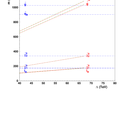
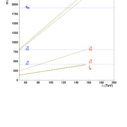
Figure 13: Sparticle masses in minimal GMSB models with $N=2$ and (a) $m_{1/2}=440$ GeV, $\tan\beta=15$ and (b) $m_{1/2}=1000$ GeV and $\tan\beta=22$, as functions of $\Lambda$ for (a) $M=800,300,200$ TeV (diagonal dashed, solid and dashed lines, respectively), and (b) $M=8000,1000,300$ TeV (diagonal dashed, solid and dashed lines, respectively), compared with GDM predictions (horizontal dot-dashed lines). The best agreement between the two models is found for (a) $\Lambda\simeq 67$ TeV and (b) $\Lambda\simeq 155$ TeV, respectively.

We have also considered the ‘average’ spectroscopic properties of GDM scenarios $\zeta$ and $\eta$, and compared them with mGMSB models with the same value of $m_{1/2}=1000$ GeV and $\tan\beta=22$. The principal discriminants we consider are again the masses of the $\chi,\chi_{2}$, ${\tilde{\ell}}_{R}$ and ${\tilde{q}}_{R}$. As in the case $m_{1/2}=440$ GeV, we again find that $N=1$ gives a ${\tilde{\ell}}_{R}$ heavier than the $\chi$, and hence can be discarded, whereas $N=3$ gives too large a mass difference $m_{\chi}-m_{{\tilde{\ell}}_{R}}$. On the other hand, as seen in panel (b) of Fig. 13, $N=2$ gives a ${\tilde{q}}_{R}$ heavier than the ${\tilde{g}}$ whereas $N=3$ again gives a lighter ${\tilde{q}}_{R}$. As in the previous case, an LHC measurement of $m_{\chi}-m_{{\tilde{\ell}}_{R}}$ has the potential to exclude mGMSB with $N=3$ and that of $m_{\tilde{g}}-m_{{\tilde{q}}_{R}}$ to exclude $N=2$.

We conclude that a combination of these mass measurements and the different lifetimes of NLSP decays would be sufficient to distinguish the GDM models of the type considered here from mGMSB models.

6.4 Stau Trapping and the Detection of Decays

If produced ${\tilde{\tau}}_{1}$’s are sufficiently slow-moving, they may be stopped inside the detector or its neighbourhood. We consider three possibilities: that the ${\tilde{\tau}}_{1}$ may be trapped inside the detector itself, or in adjacent water tank or calorimetric detector, or in the walls of the experimental cavern. In the case of the LHC, the trapping rate can be calculated using the spectra shown in Fig. 10 and the known rates of energy loss by charged particles passing though different types of matter [46]. As representative examples, we consider Iron - as in an experimental calorimeter - and Carbon - which has similar stopping power to water and less than any other plausible detector and/or surrounding material.

We display in Table 7 the numbers of ${\tilde{\tau}}_{1}$’s expected to be produced in GDM benchmark scenarios $\epsilon,\zeta,\eta$ at the LHC with 100 fb^-1 of integrated luminosity, using the cross sections shown in Table 6 calculated with PROSPINO [40]. We consider numbers of particles produced with $\beta\gamma<0.25(0.5)$ and show in each case the corresponding ranges in Carbon and Iron.

Model	$\epsilon$	$\zeta$	$\eta$
Number of particles with	850	7	7
$\beta\gamma<0.25$
Range in C (cm)	60	136	129
Range in Fe (cm)	29	65	61
Number of particles with	7700	100	90
$\beta\gamma<0.5$
Range in C (cm)	600	1360	1290
Range in Fe (cm)	290	650	610

Table 7: Numbers of slow-moving ${\tilde{\tau}}_{1}$’s produced with 100/fb at the LHC in GDM benchmark scenarios $\epsilon,\zeta,\eta$, and the corresponding ranges in Carbon and Iron.

Benchmark scenario $\epsilon$ is in a different class from scenarios $\zeta,\eta$. The numbers of slow-moving particles are orders of magnitude larger, and secondly the ranges are shorter typically by a factor of two. Both these features are directly related to the sparticle mass scale, which is set essentially by $m_{1/2}$. In the case of benchmark $\epsilon$, hundreds of ${\tilde{\tau}}_{1}$’s would be trapped within either the ATLAS or CMS calorimeter, and thousands more would be trapped within a few metres of surrounding material. On the other hand, in the cases of scenarios $\zeta,\eta$, only a handful of particles would be trapped within either detector, and only a few dozen events would be trapped within $\sim 10$ m of surrounding material.

The situation at the ILC would be very favourable for any of the scenarios considered. The above reference values of $\beta\gamma$ correspond to $\sqrt{s}=2m_{{\tilde{\tau}}_{1}}\times 1.0625(1.25)$, and there should be no problem tuning the beam energy very close to the ${\tilde{\tau}}_{1}$ mass and obtaining large samples of ${\tilde{\tau}}_{1}$’s stopped within the calorimeter. The same would be true at CLIC for mSUGRA GDM models with $m_{1/2}<4.5$ TeV.

In the case of the LHC, unfortunately there is very little room left in the ATLAS cavern for a trapping water tank or calorimeter, and it would be difficult to envisage inserting any detector over a metre thick between the barrel and the cavern walls. On the other hand, in the case of CMS there may be some more room after restructuring the infrastructure (balconies and services), permitting the installation of an ${\cal O}$(kton) trapping detector, as discussed in [47]. There would be more room in the forward direction at CMS, but this possibility would have limited angular acceptance. Moreover, the ${\tilde{\tau}}_{1}$ pseudorapidity distributions are generally very central, within the ATLAS or CMS acceptance, as shown in Figs. 5, 6, 7, so a forward trap would not be very efficient. In the case of the ILC or CLIC, if the experiments at the LHC reveal interest, it would be possible to design the experimental areas ahead of time so as to allow for a trapping detector.

In the interim, we speculate on the alternative possibility of looking for the decays of ${\tilde{\tau}}_{1}$’s that are trapped in the walls of the ATLAS and CMS caverns. One possible strategy would be to use the tracking information from CMS or ATLAS to determine the ${\tilde{\tau}}_{1}$’s impact point and angle, then bore a hole into the wall and extract a core with an optimal chance of containing a trapped ${\tilde{\tau}}_{1}$. The tracking systems of CMS and ATLAS should each yield an experimental uncertainty in the impact point that is about half a cm, and a corresponding angular error $\sim 10^{-3}$ radians. Using the standard formula [46]

$$\theta_{0}=\frac{13.6~{}{\rm MeV}}{\beta p}\sqrt{\frac{x}{X_{0}}}\{1+0.038~{}{\rm ln}(x/X_{0})\}$$ (8)

for the 98 % C.L. width of the projected distribution of the multiple scattering angle, where $\beta,p$ are the ${\tilde{\tau}}_{1}$ velocity and momentum and $x$ the penetration depth relative to the scattering length $X_{0}$, we find typical values $\theta_{0}<10^{-3}$, within the experimental angular error. As we can see from Table 7, one might want to extract ${\cal O}(100)$ to ${\cal O}(10000)$ ‘interesting’ cores with dimensions $\sim 1$ cm $\times 1$ cm $\times 10$ m each year. This technique might be appropriate for the upper part of the mSUGRA wedge shown in Fig. 1, where the ${\tilde{\tau}}_{1}$ lifetime is measured in weeks, such as scenarios $\epsilon,\zeta$. However, this is unlikely to be feasible in the lower part of the mSUGRA wedge, e.g., at point $\eta$, because radiation levels in the LHC caverns would preclude access on the necessary time-scale $\tau_{{\tilde{\tau}}_{1}}\sim 5$ hours.

The baseline operating plan for the LHC foresees one multi-month stop each winter, and half-a-dozen two-day technical stops at regular intervals during the rest of the year. Each of these would provide an opportunity to extract a limited number of cores from the cavern walls. This would be interesting if the ${\tilde{\tau}}_{1}$ lifetime is several weeks or more, as in benchmarks $\epsilon,\zeta$, but not point $\eta$.

We have also considered the possibility of measuring directly the mass of a stopped ${\tilde{\tau}}_{1}$ in a mass spectrometer. A typical extracted core of size 1 cm $\times$ 1 cm $\times$ 10 m would contain $\sim 1\times 10^{28}$ protons. On the basis of estimates of the mass of the ${\tilde{\tau}}_{1}$ and the velocity of the specific particle being sought in the core, we estimate that a ‘high-interest’ sample of about 10 % of the length of each core might be selected for exploration in more detail using a mass spectrometer. For comparison, we note that the best available upper limit on the relative abundance in water of a positively-charged stable relic particle with mass between 40 and 400 GeV is $1\times 10^{-29}$ [48]. It might therefore be feasible to pass the high-interest samples of each core through a mass spectrometer and measure the ${\tilde{\tau}}_{1}$ mass very precisely. The issue would be how quickly this study could be completed, in comparison with the ${\tilde{\tau}}_{1}$ lifetime, as discussed above.

Another possibility might be to look for upward- or sideways-going muons coming out of the wall, produced by ${\tilde{\tau}}_{1}$ decays in the neighbouring rock. We estimate that typical muon momenta would be tens of GeV, in which case they should be able to traverse tens of metres of rock. However, the acceptance for decays back into the cavern would not be large unless the ${\tilde{\tau}}_{1}$ decays within a few metres of the cavern wall. In the benchmarks studied, detecting these might be feasible for the thousands of ${\tilde{\tau}}_{1}$’s produced with $\beta\gamma<0.5$ in scenario $\epsilon$, but looks very marginal for the few dozen ${\tilde{\tau}}_{1}$’s produced with $\beta\gamma<0.5$ in scenarios $\zeta,\eta$, which would also have longer ranges, diminishing the angular acceptance for the decays.

We have compared the possible measurement of the ‘albedo’ due to ${\tilde{\tau}}_{1}\to\tau\to\mu$ decay, which has a branching ratio of $\sim 16$ %, with the irreducible background due to the known atmospheric $\nu\to\mu$ flux. Assuming that the gravitino mass is small compared with $m_{{\tilde{\tau}}_{1}}$, the characteristic $\mu$ energy will be $\sim m_{{\tilde{\tau}}_{1}}/6$, corresponding to $\sim 25$ GeV for point $\epsilon$ and $\sim 50$ GeV for points $\epsilon,\zeta$. If we consider a representative LHC or ILC detector with linear dimensions 20 m $\times$ 20 m and ${\tilde{\tau}}_{1}$ decay at a characteristic distance $\sim 10$ m, the detector subtends 1/6 of the total solid angle, namely ${2\pi\over 3}$ steradians. However, ${\tilde{\tau}}_{1}$ decays in the upper hemisphere surrounding the detector will surely be drowned in cosmic-ray $\mu$ background, so we consider only ${\tilde{\tau}}_{1}$ decays in the lower hemisphere. Therefore, only 1/12 of the decay muons are in principle observable, corresponding to just 1.3 % of the stopped ${\tilde{\tau}}_{1}$ decays. As seen from Table 7, at the LHC this would give ${\cal O}(100)$ events in benchmark scenario $\epsilon$, but only ${\cal O}(1)$ event in either of scenarios $\zeta,\eta$. For comparison, the MACRO experiment [49] has reported a sample of about 900 upward-going atmospheric $\nu\to\mu$ events passing through a detector of area 76 m $\times$ 12 m in five years of operation, corresponding to $\sim 80$ events/year through our nominal 20 m $\times$ 20 m collider detector. The energy spectrum of the MACRO ‘up-through’ $\mu$ sample has a broad peak around 50 GeV, so there is no clear separation in energy between the ${\tilde{\tau}}_{1}\to\tau\to\mu$ signal and the atmospheric $\nu\to\mu$ background. On the other hand, the tracking system defines the direction in which a candidate ${\tilde{\tau}}_{1}$ exited the detector, and the momentum measurement constrains the distance at which it is likely to have stopped. Together, these measurements define the direction from which a candidate ‘albedo’ decay muon might emerge from the wall into any part of the detector. Using this information, it might be possible to detect the ‘albedo’ decay muons at the LHC in scenario $\epsilon$, though not in scenarios $\zeta,\eta$. On the other hand, detection at the ILC could be optimized with a dedicated detector.

Comparing the mSUGRA spectra for benchmark scenarios $\epsilon,\zeta,\eta$ with the sample of GMSB models in [43], we see that there exist GMSB models with identical values of $(m_{{\tilde{\tau}}_{1}},\langle m_{\tilde{q}}\rangle)$. We are therefore pessimistic that these spectroscopic measurements at the LHC will be enough alone to distinguish mSUGRA from GMSB.

We have also considered the possibility of using ${\tilde{\tau}}_{1}\to\tau{\tilde{G}}$ decay kinematics to constrain directly the mass of the gravitino ${\tilde{G}}$, and hence perhaps also distinguish between mSUGRA and GMSB scenarios. In the three ${\tilde{\tau}}_{1}$ NLSP scenarios $\epsilon,\zeta,\eta$ considered here, the mean $\tau$ energies are $\langle E_{\tau}\rangle=74,155,160$ GeV, respectively. On the other hand, in GMSB scenarios with the same values of $m_{{\tilde{\tau}}_{1}}$, one would have $\langle E_{\tau}\rangle=75,170,161$ GeV, respectively. We recall that $m_{{\tilde{\tau}}_{1}}$ would be measurable with an accuracy that is probably not much better than 1 %, which already removes any chance of measuring the percentage difference in $\langle E_{\tau}\rangle$ in scenarios $\epsilon,\eta$, where it is ${\cal O}(1)$ %. On the other hand, the percentage difference in scenario $\zeta$ is about 10 %, which should be measurable in principle with enough events and accurate energy measurements. However, in practice, as we have discussed above, a sample size of more than 100 ${\tilde{\tau}}_{1}$ decays, as would be required for a 10 % measurement of $\langle E_{\tau}\rangle$ in scenario $\zeta$, even if $E_{\tau}$ could be measured perfectly event-by-event, could not be obtained inside ATLAS or CMS with the 100 fb^-1 integrated luminosity assumed here.

On the other hand, at the ILC $m_{{\tilde{\tau}}_{1}}$ should be measurable with an accuracy better than 0.1 %, and it should be possible to obtain a large enough sample to measure $\langle E_{\tau}\rangle$ with an accuracy of a few %. We therefore think that distinguishing scenario $\zeta$ from a GMSB model with the same $m_{{\tilde{\tau}}_{1}}$ should be possible, but making the same distinction for scenarios $\zeta,\eta$ would be much more challenging, in view of the very accurate $\langle E_{\tau}\rangle$ measurement required.

7 Conclusions

We have discussed in this paper various alternatives to the constrained MSSM (CMSSM) framework with universal soft supersymmetry breaking, which has been used in most previous benchmark studies of supersymmetric signatures at the LHC, ILC and CLIC. Specifically, we have considered both a less constrained framework with non-universal Higgs masses (NUHM) and a more constrained gravitino dark matter (GDM) framework inspired by minimal supergravity (mSUGRA). As we have shown, both of these scenarios offer distinctive phenomenological signatures that were absent in the previous CMSSM studies, at least when cosmological constraints from WMAP and other experiments were taken into account. For example, Gravitino Dark Matter (GDM) becomes a generic possibility.

In the case of NUHM models, the freedom to vary the scalar masses relative to the gaugino mass $m_{1/2}$ opens up the possibility of different characteristic heavier neutralino decays such as $\chi_{2}\to\chi h,\chi Z$, which were disfavoured along the WMAP lines allowed in the CMSSM. Three of the new benchmark scenarios we have proposed and examined here are of this type. One has a dominant $\chi_{2}\to\chi Z$ decay mode (point $\alpha$), one has a dominant $\chi_{2}\to\chi h$ decay mode (point $\beta$), and one has non-resonant $\chi_{2}\to\chi\ell^{+}\ell^{-}$ decays (point $\gamma$). The $h$ signal at point $\beta$ should easily be detected at the LHC, and a fortiori at the ILC or CLIC. These features open up new possibilities for reconstructing the cascade decays of heavier sparticles and measuring better the mass of the lightest neutralino $\chi$.

In the case of GDM models, there are two generic possibilities for the next-to-lightest supersymmetric particle (NLSP). Either it is neutral and presumably the lightest neutralino $\chi$, as exemplified by benchmark scenario $\delta$, or it is charged and presumably the lighter stau slepton ${\tilde{\tau}}_{1}$, as exemplified by benchmark scenarios $\epsilon,\zeta$ and $\eta$.

In the former case, which is a CMSSM scenario with the gravitino specifically chosen to be light, the collider signatures are very similar to those for scenarios with a stable $\chi$, since generic decays of the unstable $\chi$ occur far outside the collider detector. However, the sparticle spectrum is somewhat different from what it would be along a WMAP line, providing an opportunity to distinguish this possibility, for example in ${\tilde{g}}\to{\tilde{b}}b$ decays.

The three benchmark scenarios $\epsilon,\zeta$ and $\eta$ with a ${\tilde{\tau}}_{1}$ NLSP span the range of possibilities that are likely to be detectable at the LHC or ILC within the mSUGRA framework. Point $\epsilon$ was chosen to have sparticles as light as possible, with heavier spectra at points $\zeta,\eta$. At point $\zeta$ the ${\tilde{\tau}}_{1}$ lifetime is close to its theoretical maximum, and at point $\eta$ the ${\tilde{\tau}}_{1}$ lifetime is close to the minimum we consider.

In all three cases, the ${\tilde{\tau}}_{1}$ should be detectable as a slowly-moving metastable particle, and TOF measurements at the LHC might enable its mass to be measured with an accuracy at the % level. We have discussed how these mSUGRA GDM scenarios could be distinguished from mGMSB models.

As pointed out in [35, 36], a small fraction of the produced ${\tilde{\tau}}_{1}$’s may be stopped inside the collider detector and/or in surrounding material, either cavern walls or a specialized stopping detector. At the LHC, there is limited space in the constructed caverns for such a specialized detector [47], but this could be envisaged in designing intersection regions for the ILC or CLIC, if needed. We have discussed a couple of strategies for detecting ${\tilde{\tau}}_{1}$’s that might have stopped in the cavern walls surrounding ATLAS or CMS, either by extracting cores from the surrounding wall material or by looking for muons from the decays ${\tilde{\tau}}_{1}\to\tau+$ gravitino followed by $\tau\to\mu+\nu_{e}{\bar{\nu}}_{\mu}$. The validities of these strategies depend on practical feasibility as well as the ${\tilde{\tau}}_{1}$ lifetime, which is uncertain by two orders of magnitude even in the restricted mSUGRA framework discussed here.

Our preliminary investigations indicate that the LHC has good capabilities to discover supersymmetry in each of the benchmark scenarios proposed, and may be able to uncover several different sparticles in each case. However, in general the LHC experiments would not be able to make many very accurate spectroscopic measurements. In several of the benchmark scenarios, an ILC with $\sqrt{s}=0.5$ TeV would already be able to make several precise measurements of weakly-interacting sparticles, and a 1 TeV ILC would extend this capability to all the benchmarks studied here. In all the scenarios studied, the additional measurements possible with CLIC at $\sqrt{s}=3$ or 5 TeV would contribute significant added value to the exploration of the new physics previously uncovered by the LHC and followed up by the ILC.

These new benchmark scenarios merely scratch the surface of the myriad possibilities open in supersymmetric phenomenology once one explores the high-dimensional parameter space of soft supersymmetry breaking. These examples should offer general encouragement to think outside the CMSSM box, and suggest the likelihood that even more exotic possibilities might be waiting out there, perhaps including one chosen by Nature.

Acknowledgments
The work of K.A.O. was supported partly by DOE grant DE–FG02–94ER–40823. We thank S. Abdullin, E. Tsesmelis, D. Forkel-Wirth, R. Voss and M. White for useful discussions.

References

- [1] L. Maiani, Proceedings of the 1979 Gif-sur-Yvette Summer School On Particle Physics, 1; G. ’t Hooft, in Recent Developments in Gauge Theories, Proceedings of the Nato Advanced Study Institute, Cargese, 1979, eds. G. ’t Hooft et al., (Plenum Press, NY, 1980); E. Witten, Phys. Lett. B 105, 267 (1981).
-
[2]
LEP Electroweak Working Group,
http://lepewwg.web.cern.ch/LEPEWWG/Welcome.html. - [3] J. Ellis, S. Kelley and D. V. Nanopoulos, Phys. Lett. B260 (1991) 131; U. Amaldi, W. de Boer and H. Furstenau, Phys. Lett. B260 (1991) 447; C. Giunti, C. W. Kim and U. W. Lee, Mod. Phys. Lett. A6 (1991) 1745.
- [4] J. R. Ellis, J. S. Hagelin, D. V. Nanopoulos, K. A. Olive and M. Srednicki, Nucl. Phys. B 238, 453 (1984); see also H. Goldberg, Phys. Rev. Lett. 50, 1419 (1983).
- [5] G. W. Bennett et al. [Muon g-2 Collaboration], Phys. Rev. Lett. 92 (2004) 161802 [arXiv:hep-ex/0401008]; M. Davier, S. Eidelman, A. Hocker and Z. Zhang, Eur. Phys. J. C 31 (2003) 503 [arXiv:hep-ph/0308213]; K. Hagiwara, A. D. Martin, D. Nomura and T. Teubner, Phys. Rev. D 69, 093003 (2004) [arXiv:hep-ph/0312250]; J. F. de Troconiz and F. J. Yndurain, Phys. Rev. D 71, 073008 (2005) [arXiv:hep-ph/0402285]; K. Melnikov and A. Vainshtein, Phys. Rev. D 70 (2004) 113006 [arXiv:hep-ph/0312226]; M. Passera, J. Phys. G 31, R75 (2005) [arXiv:hep-ph/0411168].
- [6] I. Hinchliffe, F. E. Paige, M. D. Shapiro, J. Soderqvist and W. Yao, Phys. Rev. D55 (1997) 5520; S. Abdullin et al. [CMS Collaboration], hep-ph/9806366; S. Abdullin and F. Charles, Nucl. Phys. B547 (1999) 60; TESLA Technical Design Report, DESY-01-011, Part III, Physics at an Linear Collider (March 2001).
- [7] M. Battaglia et al., Eur. Phys. J. C 22, 535 (2001) [arXiv:hep-ph/0106204].
- [8] B. C. Allanach et al., Proc. of the APS/DPF/DPB Summer Study on the Future of Particle Physics (Snowmass 2001) ed. N. Graf, Eur. Phys. J. C 25 (2002) 113 [eConf C010630 (2001) P125] [arXiv:hep-ph/0202233]; G. L. Kane, J. Lykken, S. Mrenna, B. D. Nelson, L. T. Wang and T. T. Wang, Phys. Rev. D 67 (2003) 045008 [arXiv:hep-ph/0209061].
- [9] M. Battaglia, A. De Roeck, J. R. Ellis, F. Gianotti, K. A. Olive and L. Pape, Eur. Phys. J. C 33 (2004) 273 [arXiv:hep-ph/0306219].
- [10] J. R. Ellis and D. V. Nanopoulos, Phys. Lett. B 110 (1982) 44; R. Barbieri and R. Gatto, Phys. Lett. B 110 (1982) 211.
- [11] V. Berezinsky, A. Bottino, J. R. Ellis, N. Fornengo, G. Mignola and S. Scopel, Astropart. Phys. 5, 1 (1996) [arXiv:hep-ph/9508249]; M. Drees, M. M. Nojiri, D. P. Roy and Y. Yamada, Phys. Rev. D 56, 276 (1997) [Erratum-ibid. D 64 (1997) 039901] [arXiv:hep-ph/9701219]; M. Drees, Y. G. Kim, M. M. Nojiri, D. Toya, K. Hasuko and T. Kobayashi, Phys. Rev. D 63, 035008 (2001) [arXiv:hep-ph/0007202]; P. Nath and R. Arnowitt, Phys. Rev. D 56, 2820 (1997) [arXiv:hep-ph/9701301]; A. Bottino, F. Donato, N. Fornengo and S. Scopel, Phys. Rev. D 63, 125003 (2001) [arXiv:hep-ph/0010203]; S. Profumo, Phys. Rev. D 68, 015006 (2003) [arXiv:hep-ph/0304071]; D. G. Cerdeno and C. Munoz, JHEP 0410, 015 (2004) [arXiv:hep-ph/0405057]; H. Baer, A. Mustafayev, S. Profumo, A. Belyaev and X. Tata, arXiv:hep-ph/0504001.
- [12] J. R. Ellis, K. Olive and Y. Santoso, Phys. Lett. B539 (2002) 107 [arXiv:hep-ph/0204192].; J. R. Ellis, T. Falk, K. A. Olive and Y. Santoso, Nucl. Phys. B652 (2003) 259 [arXiv:hep-ph/0210205].
- [13] J. R. Ellis, J. E. Kim and D. V. Nanopoulos, Phys. Lett. B 145 (1984) 181; T. Moroi, H. Murayama and M. Yamaguchi, Phys. Lett. B 303 (1993) 289; J. R. Ellis, D. V. Nanopoulos, K. A. Olive and S. J. Rey, Astropart. Phys. 4 (1996) 371 [arXiv:hep-ph/9505438]; M. Bolz, W. Buchmuller and M. Plumacher, Phys. Lett. B 443 (1998) 209 [arXiv:hep-ph/9809381]; T. Gherghetta, G. F. Giudice and A. Riotto, Phys. Lett. B 446 (1999) 28 [arXiv:hep-ph/9808401]; T. Asaka, K. Hamaguchi and K. Suzuki, Phys. Lett. B 490 (2000) 136 [arXiv:hep-ph/0005136]; M. Fujii and T. Yanagida, Phys. Rev. D 66 (2002) 123515 [arXiv:hep-ph/0207339]; Phys. Lett. B 549 (2002) 273 [arXiv:hep-ph/0208191].
- [14] M. Bolz, A. Brandenburg and W. Buchmuller, Nucl. Phys. B 606 (2001) 518 [arXiv:hep-ph/0012052]; W. Buchmuller, K. Hamaguchi and M. Ratz, Phys. Lett. B 574 (2003) 156 [arXiv:hep-ph/0307181].
- [15] J. R. Ellis, K. A. Olive, Y. Santoso and V. C. Spanos, Phys. Lett. B 588 (2004) 7 [arXiv:hep-ph/0312262].
- [16] J J. L. Feng, S. Su and F. Takayama, Phys. Rev. D 70, 075019 (2004) [arXiv:hep-ph/0404231]; J. L. Feng, S. f. Su and F. Takayama, Phys. Rev. D 70, 063514 (2004) [arXiv:hep-ph/0404198]; J. L. Feng, A. Rajaraman and F. Takayama, Phys. Rev. Lett. 91 (2003) 011302 [arXiv:hep-ph/0302215].
- [17] H. P. Nilles, Phys. Rept. 110 (1984) 1.
- [18] J. R. Ellis, K. A. Olive, Y. Santoso and V. C. Spanos, Phys. Lett. B573 (2003) 162 [arXiv:hep-ph/0305212]; Phys. Rev. D70 (2004) 055005 [arXiv:hep-ph/0405110].
- [19] J. Polonyi, Budapest preprint KFKI-1977-93 (1977); R. Barbieri, S. Ferrara and C.A. Savoy, Phys. Lett. 119B (1982) 343.
- [20] Information about this code is available from K. A. Olive: it contains important contributions from T. Falk, G. Ganis, J. McDonald, K. A. Olive, Y. Santoso and M. Srednicki.
- [21] We use mainly the 7.69 version of ISASUGRA, whose basic documentation is found in H. Baer, F. E. Paige, S. D. Protopopescu and X. Tata, ISAJET 7.48: A Monte Carlo event generator for , , and reactions, hep-ph/0001086. The latest update is available from http://paige.home.cern.ch/paige/.
- [22] J. R. Ellis, T. Falk, G. Ganis, K. A. Olive and M. Srednicki, Phys. Lett. B510, 236 (2001) [arXiv:hep-ph/0102098]; J. R. Ellis, K. A. Olive and Y. Santoso, New Jour. Phys. 4 (2002) 32 [arXiv:hep-ph/0202110]; J. R. Ellis, K. A. Olive, Y. Santoso and V. C. Spanos, Phys. Lett. B 565 (2003) 176 [arXiv:hep-ph/0303043]; J. R. Ellis, K. A. Olive, Y. Santoso and V. C. Spanos, Phys. Rev. D 69 (2004) 095004 [arXiv:hep-ph/0310356].
- [23] V. D. Barger and C. Kao, Phys. Lett. B 518 (2001) 117 [arXiv:hep-ph/0106189]; L. Roszkowski, R. Ruiz de Austri and T. Nihei, JHEP 0108 (2001) 024 [arXiv:hep-ph/0106334]; A. B. Lahanas and V. C. Spanos, Eur. Phys. J. C 23 (2002) 185 [arXiv:hep-ph/0106345]; H. Baer, C. Balazs, A. Belyaev, J. K. Mizukoshi, X. Tata and Y. Wang, JHEP 0207 (2002) 050 [arXiv:hep-ph/0205325]; R. Arnowitt and B. Dutta, arXiv:hep-ph/0211417. H. Baer and C. Balazs, JCAP 0305 (2003) 006 [arXiv:hep-ph/0303114]; H. Baer, C. Balazs, A. Belyaev, T. Krupovnickas and X. Tata, JHEP 0306 (2003) 054 [arXiv:hep-ph/0304303]; A. B. Lahanas and D. V. Nanopoulos, Phys. Lett. B 568 (2003) 55 [arXiv:hep-ph/0303130]; U. Chattopadhyay, A. Corsetti and P. Nath, Phys. Rev. D 68 (2003) 035005 [arXiv:hep-ph/0303201]; C. Munoz, arXiv:hep-ph/0309346.
- [24] S. Chen et al. [CLEO Collaboration], Phys. Rev. Lett. 87 (2001) 251807 [arXiv:hep-ex/0108032]; P. Koppenburg et al. [Belle Collaboration], Phys. Rev. Lett. 93 (2004) 061803 [arXiv:hep-ex/0403004]. B. Aubert et al. [BaBar Collaboration], arXiv:hep-ex/0207076; M. Ciuchini, G. Degrassi, P. Gambino and G. F. Giudice, Nucl. Phys. B 527 (1998) 21 [arXiv:hep-ph/9710335]; Nucl. Phys. B 534 (1998) 3 [arXiv:hep-ph/9806308]; C. Degrassi, P. Gambino and G. F. Giudice, JHEP 0012 (2000) 009 [arXiv:hep-ph/0009337]; M. Carena, D. Garcia, U. Nierste and C. E. Wagner, Phys. Lett. B 499 (2001) 141 [arXiv:hep-ph/0010003]; P. Gambino and M. Misiak, Nucl. Phys. B 611 (2001) 338; D. A. Demir and K. A. Olive, Phys. Rev. D 65 (2002) 034007 [arXiv:hep-ph/0107329]; F. Borzumati, C. Greub and Y. Yamada, Phys. Rev. D 69 (2004) 055005 [arXiv:hep-ph/0311151]; T. Hurth, Rev. Mod. Phys. 75 (2003) 1159 [arXiv:hep-ph/0212304].
- [25] J. R. Ellis, S. Heinemeyer, K. A. Olive and G. Weiglein, JHEP 0502 (2005) 013 [arXiv:hep-ph/0411216].
- [26] ATLAS Collaboration, ATLAS detector and physics performance Technical Design Report, CERN/LHCC 99-14/15 (1999).
- [27] CMS Collaboration, Technical Proposal, CERN/LHCC 94-38 (1994).
- [28] S. Matsumoto et al. [JLC Group], JLC-1, KEK Report 92-16 (1992); J. Bagger et al. [American Linear Collider Working Group], The Case for a 500-GeV Linear Collider, SLAC-PUB-8495, BNL-67545, FERMILAB-PUB-00-152, LBNL-46299, UCRL-ID-139524, LBL-46299, Jul 2000, arXiv:hep-ex/0007022; T. Abe et al. [American Linear Collider Working Group Collaboration], Linear Collider Physics Resource Book for Snowmass 2001, SLAC-570, arXiv:hep-ex/0106055, hep-ex/0106056, hep-ex/0106057 and hep-ex/0106058; TESLA Technical Design Report, DESY-01-011, Part III, Physics at an Linear Collider (March 2001).
- [29] R. W. Assmann et al. [CLIC Study Team], A 3-TeV Linear Collider Based on CLIC Technology, ed. G. Guignard, CERN 2000-08; for more information about this project, see: http://ps-div.web.cern.ch/ps-div/CLIC/Welcome.html; CLIC Physics Study Group, http://clicphysics.web.cern.ch/CLICphysics/ and Yellow Report in preparation.
-
[30]
Joint LEP 2 Supersymmetry Working Group,
Combined LEP Chargino Results, up to 208 GeV,
http://lepsusy.web.cern.ch/lepsusy/www/inos_moriond01/ charginos_pub.html; Combined LEP Selectron/Smuon/Stau Results, 183-208 GeV,
http://lepsusy.web.cern.ch/lepsusy/www/sleptons_summer02/ slep_2002.html. - [31] LEP Higgs Working Group for Higgs boson searches, OPAL Collaboration, ALEPH Collaboration, DELPHI Collaboration and L3 Collaboration, Search for the Standard Model Higgs Boson at LEP, CERN-EP/2003-011, arXiv:hep-ex/0306033.
- [32] C. L. Bennett et al., Astrophys. J. Suppl. 148 (2003) 1; D. N. Spergel et al., Astrophys. J. Suppl. 148 (2003) 175.
-
[33]
The CDF Collaboration, the D0 Collaboration and the Tevatron Electroweak
Working Group,
arXiv:hep-ex/0507091;
this supersedes
arXiv:hep-ex/0507006;
V. Abazov et al. [D0 Collaboration],
Nature 429 (2004) 638,
hep-ex/0406031;
P. Azzi et al. [CDF Collaboration, D0 Collaboration], hep-ex/0404010. - [34] R. H. Cyburt, J. R. Ellis, B. D. Fields and K. A. Olive, Phys. Rev. D 67, 103521 (2003) [arXiv:astro-ph/0211258]; J. R. Ellis, K. A. Olive and E. Vangioni, arXiv:astro-ph/0503023; for another treatment, see K. Kohri, T. Moroi and A. Yotsuyanagi, arXiv:hep-ph/0507245 and references therein.
- [35] K. Hamaguchi, Y. Kuno, T. Nakaya and M. M. Nojiri, Phys. Rev. D 70 (2004) 115007 [arXiv:hep-ph/0409248].
- [36] J. L. Feng and B. T. Smith, Phys. Rev. D 71 (2005) 015004 [Erratum-ibid. D 71 (2005) 0109904] [arXiv:hep-ph/0409278].
- [37] T. Sjostrand, L. Lonnblad and S. Mrenna, arXiv:hep-ph/0108264.
- [38] CMS Physics Technical Design Report, in preparation.
- [39] S. Heinemeyer, W. Hollik and G. Weiglein, Comput. Phys. Commun. 124 (2000) 76 [hep-ph/9812320] and Eur. Phys. J. C 9 (1999) 343 [arXiv:hep-ph/9812472].
- [40] W. Beenakker, R. Hopker and M. Spira, arXiv:hep-ph/9611232.
- [41] See [26, 27], and the second and third papers in [6].
- [42] S. Berge and M. Klasen, Eur. Phys. J. C 30 (2003) 123 [arXiv:hep-ph/0303032].
- [43] For a review, see: G. F. Giudice and R. Rattazzi, Phys. Rept. 322 (1999) 419 [arXiv:hep-ph/9801271].
- [44] S. Ambrosanio, B. Mele, S. Petrarca, G. Polesello and A. Rimoldi, JHEP 0101 (2001) 014 [arXiv:hep-ph/0010081].
- [45] D. Treille, private communication.
- [46] S. Eidelman et al., Phys. Lett. B 592, 1 (2004).
- [47] K. Hamaguchi, M. Nojiri and A. De Roeck, in preparation.
- [48] P. F. Smith, J. R. J. Bennett, G. J. Homer, J. D. Lewin, H. E. Walford and W. A. Smith, Nucl. Phys. B 206 (1982) 333.
- [49] M. Ambrosio et al. [MACRO Collaboration], Eur. Phys. J. C 36 (2004) 323.