MSU-HEP-050816

Light-Cone Models for Intrinsic Charm and Bottom

Jon Pumplin

Department of Physics and Astronomy

Michigan State University, E. Lansing, MI 48824

Expectations for the momentum distribution of nonperturbative charm and bottom quarks in the proton are derived from a variety of models for the Fock space wave function on the light cone.

Keywords: intrinsic charm, light cone, heavy quarks, parton distributions

1 Introduction

Interactions of hadrons at high energy—such as those probed in $\mathrm{ep}$ scattering at HERA, $\bar{\mathrm{p}}\mathrm{p}$ scattering at the Tevatron, and $\mathrm{pp}$ scattering at the forthcoming LHC—are to be understood in terms of the interactions of their quark and gluon constituents. The parton distribution functions (PDFs) that describe the proton’s quark and gluon content are therefore essential for testing the Standard Model and searching for New Physics.

The PDFs are functions $f_{a}(x,\mu)$ where $x$ is the fraction of the proton’s momentum carried by parton species $a$ at scale $\mu$, in a frame where that momentum is large. For small values of $\mu$, corresponding to long distance scales, the PDFs express nonperturbative physics that is beyond the scope of present calculations from first principles in QCD (although some progress has been made using lattice methods [1]). Current practice is instead to parametrize the PDFs at a scale $\mu_{0}$ that is large enough for ${f_{a}(x,\mu)}$ to be calculated from ${f_{a}(x,\mu_{0})}$ at all $\mu>\mu_{0}$ by perturbation theory. The unknown functions $f_{a}(x,\mu_{0})$ are determined empirically by adjusting their parameters to fit a large variety of data at $\mu>\mu_{0}$ in a “QCD global analysis” [2, 3].

A number of important processes, including Higgs boson production in certain scenarios, are particularly sensitive to the bottom or charm quark distributions $f_{c}(x,\mu)$ and $f_{b}(x,\mu)$. In the global analyses that have been carried out so far, it is assumed that the charm content of the proton is negligible at $\mu\!\sim\!m_{c}$, and similarly that bottom is negligible at $\mu\!\sim\!m_{b}$, so these heavy quark components arise only perturbatively through gluon splitting in the DGLAP evolution. The global fits are not inconsistent with this assumption, but the data sets they are based on do not yet include experiments that are strongly sensitive to heavy quarks, so substantially larger $c$ or $b$ content cannot be ruled out. Direct measurements of $c$ and $b$ production in deep inelastic scattering are also consistent with an entirely perturbative origin for heavy quark flavors [4], but those experiments are not sensitive to heavy quarks at large $x$.

Meanwhile, in the light-cone Fock space picture [5], it is natural to expect nonperturbative “intrinsic” heavy quark components in the proton wave function [6, 7]. Furthermore, $s$ and $\bar{s}$ quarks each carry $\sim\!1\%$ of the proton momentum at $\mu_{0}=1.3\,\mathrm{GeV}$ [2], which implies that states made of $uuds\bar{s}$, together with gluons, make up a significant component of the proton wave function. By analogy, one would expect $uudc\bar{c}$ and $uudb\bar{b}$ also to be present—although the degree of suppression caused by greater off-shell distances is difficult to predict. A suppression as mild as $\sim 1/m_{c}^{2}$ has been derived using a semiclassical approximation for the heavy quark fields [8].

An alternative way to describe the proton in light-cone Fock space is in terms of off-shell physical particles—the “meson cloud” picture [9, 10, 11]. Specifically, the two-body state $\overline{D}^{0}\Lambda_{c}^{+}$, where $\overline{D}^{0}$ is a $u\bar{c}$ meson and $\Lambda_{c}^{+}$ is a $udc$ baryon, forms a natural low-mass component. This is the flavor $SU(4)$ analog of the $K^{+}\Lambda^{0}$ component that is a natural source of strangeness, and in particular of $f_{s}(x,\mu)\neq f_{\bar{s}}(x,\mu)$ [12]. A charm contribution from the two-body state $p\,J\!/\!\psi$ is also possible.

The light-cone view is not developed to a point where the normalization of $uudc\bar{c}$ and $uudb\bar{b}$ components can be calculated with any confidence, though estimates on the order of $1\%$ have been found for intrinsic charm (IC) using a meson cloud model [9], the MIT bag model [13], and an SU(4) quark model [14]. However, we can use the picture to predict the $x$-dependence of the non-perturbative contribution. A central feature of the light-cone models is that heavy quarks appear mainly at large $x$, because their contribution to the off-shell distance is proportional to $(p_{\perp}^{\,2}+m^{2})/x$, so the suppression of far off-shell configurations favors large $x$ when $m$ is large. We will show that this feature leads to similar predictions for the shape in $x$ from a wide variety of specific models.

Using the rough consensus of the models as a guide to the shape of $x$-dependence for intrinsic charm and bottom, it will be possible to estimate their normalization from a limited set of data. This will be carried out in a future publication. When more complete data become available, such as jet measurements with $c$- and $b$-tagging (either inclusive jets or jets produced in association with $W$, $Z$, or $\gamma$), it will become possible to extract the $x$-dependence empirically. It will then be interesting to see if the model predictions for the $x$-dependence are borne out.

Models in which the $uudc\bar{c}$ Fock space component is considered directly are described in Sec. 2. Models based on low-mass meson+baryon pairs are described in Sec. 3. The model results are compared with expectations for perturbatively generated heavy quarks in Sec. 4. The model results are compared with the light quark and gluon distributions in Sec. 5. Conclusions are summarized in Sec. 6, where simple parametrizations of all of the model predictions are tabulated for convenience in later work. The connection between the light-cone description and ordinary Feynman diagrams, which is used in Secs. 2 and 3, is derived in an Appendix.

2 Five-quark models

The probability distribution for the 5-quark state $uudc\bar{c}$ in the light-cone description of the proton can be written as

$$dP={\mathcal{N}}\,\prod_{j=1}^{5}\!{{dx_{j}}\over{x_{j}}}\,\delta(1-\sum_{j=1}^{5}x_{j})\,\prod_{j=1}^{5}\!d^{2}p_{j{\scriptscriptstyle\perp}}\,\delta^{(2)}(\sum_{j=1}^{5}p_{j{\scriptscriptstyle\perp}})\,{{F^{2}}\over{(s-m_{0}^{\,2})^{2}}}\;,$$ (1)

where

$$s=\sum_{j=1}^{5}(p_{j{\scriptscriptstyle\perp}}^{\,2}\,+\,m_{j}^{\,2})/x_{j}$$ (2)

and ${\mathcal{N}}$ is a normalization constant. Eq. (1) contains a wave function factor $F^{2}$ that characterizes the dynamics of the bound state. This factor must suppress contributions from large values of $s$ to make the integrated probability converge. An elementary derivation of Eq. (1) is given in the Appendix.

2.1 The BHPS model

A simple model for the $x$-dependence of charm can be obtained by neglecting the $p_{\perp}$ content, the $1/x_{j}$ factors, and $F^{2}$ in Eq. (1). Further approximating the charm quark mass as large compared to all the other masses yields

$$dP\propto\prod_{j=1}^{5}dx_{j}\,\delta(1-\sum_{j=1}^{5}x_{j})\,(1/x_{4}+1/x_{5})^{-2}\;,$$ (3)

where $x_{4}=x_{c}$ and $x_{5}=x_{\bar{c}}$. Carrying out all but one of the integrals and normalizing to an assumed total probability of $1\%$ yields

$${{dP}\over{dx}}=f_{c}(x)=f_{\bar{c}}(x)=6\,x^{2}\left[6\,x\,(1+x)\,\ln x\,+\,(1-x)(1+10x+x^{2})\right]\;,$$ (4)

where $x=x_{c}$ or $x_{\bar{c}}\,$. Equation (4) was first derived by Brodsky, Hoyer, Peterson and Sakai [6], and has been used many times since. We will use this BHPS model as a convenient reference for comparing all other models.

Charm distributions that arise when the transverse momentum content of Eq. (1) is not deleted are derived in the following subsections.

Figure 1: Momentum distribution of $c$ or $\bar{c}$ from the 5-quark model with the exponential suppression of Eq. (5) (left), or the power-law suppression of Eq. (6) (right). Solid curves are the BHPS model of Eq. (4). All curves are normalized to $1\%$ integrated probability.

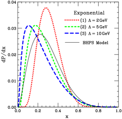
2.2 Exponential suppression

A plausible conjecture would be that high-mass configurations in Eq. (1) are suppressed by a factor

$$F^{2}=e^{-(s-m_{0}^{\,2})/\Lambda^{2}}\;.$$ (5)

This exponential form makes the total probability integral converge for any number of constituents, while a power law would not (see Eq. (21) in the Appendix).

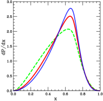
Figure 1(a) shows the charm distribution for several choices of the parameter $\Lambda$ in Eq. (5). The mass values used were $m_{0}=0.938\,\mathrm{GeV}$ and $m_{4}=m_{5}=1.5\,\mathrm{GeV}$. Constituent quark masses $m_{1}=m_{2}=m_{3}=m_{0}/3$ were used for the light quarks, but even setting those masses to zero instead yields very similar results. All curves are normalized to $1\%$ integrated probability. The results are qualitatively similar to the BHPS model, but are somewhat smaller in the region $x>0.5$, which is the most important region as shown in Sec. 5.

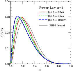
2.3 Power-Law suppression

Alternatively, we might assume that high-mass five-quark states are suppressed only by a power law, say

$$F^{2}\propto(s+\Lambda^{2})^{-n}\;.$$ (6)

Figure 1(b) shows the charm distribution for several choices of the parameter $\Lambda$ with $n=4$. The results are again rather similar to the BHPS model, and again smaller than that model at large $x$. This behavior is fairly insensitive to the choice of $n$: similar results were found for $n=3$ (not shown), while large values of $n$ revert to the exponential form of Section 2.2. Values $n\leq 2$ are unphysical, since they would make the total probability diverge. The value $n=3$ is perhaps the most natural, since it leads to a dependence $\sim 1/m_{c}^{2}$ that is in line with the result of [8].

Figure 2: Momentum distribution of $c$ and $\bar{c}$ from the $(udc)(u\bar{c})$ model (7), and $c=\bar{c}$ from the $(uud)(c\bar{c})$ model (10).

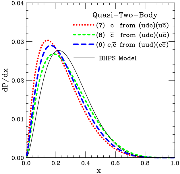
2.4 Quasi-Two-body suppression

Another approach to the suppression of high-mass Fock space components can be made on the basis of quasi-two-body states, such as those that will be considered explicitly in Section 3. For instance, we might assume the relevant 5-quark configurations are grouped as $(udc)(u\bar{c})$, in which case a plausible wave function factor would be

$$F^{2}\propto(s_{124}+\Lambda_{124}^{\;2})^{-2}\times(s_{35}+\Lambda_{35}^{\,2})^{-2}$$ (7)

where

$$s_{124} = (p_{1{\scriptscriptstyle\perp}}^{\,2}+m_{1}^{\,2})/x_{1}\,+\,(p_{2{\scriptscriptstyle\perp}}^{\,2}+m_{2}^{\,2})/x_{2}\,+\,(p_{4{\scriptscriptstyle\perp}}^{\,2}+m_{4}^{\,2})/x_{4}$$ (8)

$$s_{35} = (p_{3{\scriptscriptstyle\perp}}^{\,2}+m_{3}^{\,2})/x_{3}\,+\,(p_{5{\scriptscriptstyle\perp}}^{\,2}+m_{5}^{\,2})/x_{5}\;.$$ (9)

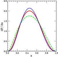
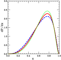
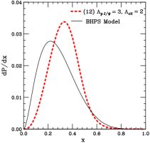
Figure 2 shows the $c$ and $\bar{c}$ distributions according to this assumption. The parameter choices were $\Lambda_{124}=2.5\,\mathrm{GeV}$ and $\Lambda_{35}=2.0\,\mathrm{GeV}$, but other plausible choices lead to similar results. Note that there is a small difference between the $c$ and $\bar{c}$ distributions in this model, with—perhaps surprisingly—$\bar{c}(x)>c(x)$ at large $x$. Observing a $\bar{c}(x)\,$–$\,c(x)$ difference would of course definitively prove a non-perturbative origin for charm.

Alternatively, we might assume the relevant 5-quark configurations are grouped as $(uud)(c\bar{c})$, so a plausible wave function factor would be

$$F^{2}\propto(s_{123}+\Lambda_{123}^{\;2})^{-2}\times(s_{45}+\Lambda_{45}^{\,2})^{-2}\;.$$ (10)

The result of this assumption with $\Lambda_{123}=1\,\mathrm{GeV}$ and $\Lambda_{45}=3\,\mathrm{GeV}$ is also shown in Fig. 2. It happens to be very similar to the average of $c$ and $\bar{c}$ from the preceding model.

Figure 3: (a) Momentum distribution of $\Lambda_{c}^{+}$ from $p\to\overline{D}^{0}\Lambda_{c}^{+}$ with $\Lambda_{p}=10$ (dashed), $4$ (solid), $2$ (dotted). (b) Momentum distribution of $c$ from $\Lambda_{c}\to udc$ with $\Lambda_{\Lambda}=4$ (dashed), $2$ (solid), $1$ (dotted). (c) Resulting distribution of $c$ in $p$ with $\Lambda_{p}=4$ and $\Lambda_{\Lambda}=2$ and BHPS model (solid).

Figure 4: (a) Momentum distribution of $\overline{D}^{0}$ from $p\to\overline{D}^{0}\Lambda_{c}^{+}$ with $\Lambda_{p}=10$ (dashed), $4$ (solid), $2$ (dotted). (b) Momentum distribution of $\bar{c}$ from $\overline{D}^{0}\to\bar{c}\,u$ with $\Lambda_{D}=4$ (dashed), $2$ (solid), $1$ (dotted). (c) Resulting distribution of $\bar{c}$ in $p$ with $\Lambda_{p}=4$ and $\Lambda_{D}=2$.

Figure 5: (a) Momentum distribution of $J\!/\!\psi$ from $p\to p\,J\!/\!\psi$ with $\Lambda_{p\,J\!/\!\psi}=5$ (dashed), $3$ (solid), $1$ (dotted). (b) Momentum distribution of $c$ or $\bar{c}$ from $J\!/\!\psi\to c\bar{c}$ with $\Lambda_{\bar{c}c}=5$ (dashed), $2$ (solid), $1$ (dotted). (c) Resulting distribution of $c$ or $\bar{c}$ in $p$ with $\Lambda_{p\,J\!/\!\psi}=3$, $\Lambda_{c\bar{c}}=2$.

3 Meson+Baryon models

Another way to picture the proton in light-cone Fock space is as a superposition of configurations of off-shell physical particles. In particular, the two-body state $\overline{D}^{0}\Lambda_{c}^{+}$, where $\overline{D}^{0}$ is a $u\bar{c}$ meson and $\Lambda_{c}^{+}$ is a $udc$ baryon, is a natural low-mass component.

We can model the $\overline{D}^{0}\Lambda_{c}^{+}$ probability distribution in the proton using Eq. (21) with $N=2$ and $F^{2}\propto(s_{D\Lambda}+\Lambda_{p}^{\,2})^{-2}\,$. The physical masses are $m_{0}=0.9383$, $m_{1}=1.8641$, and $m_{2}=2.2849$ in $\mathrm{GeV}$. We then model the $udc$ distribution in $\Lambda_{c}^{+}$ similarly, using $N=3$ and $F^{2}\propto(s_{udc}+\Lambda_{\Lambda}^{\,2})^{-2}$, with $m_{0}=2.2849$, $m_{1}=m_{2}=0.938/3$, and $m_{3}=1.6\,$. We similarly model the $u\bar{c}$ distribution in $\overline{D}^{0}$ using $N=2$ and $F^{2}\propto(s_{u\bar{c}}+\Lambda_{D}^{\,2})^{-2}$, with $m_{0}=1.8641$ and $m_{1}=m_{2}=1.60\,$. (The charm quark mass here must be taken $>\!1.55$ to keep $m_{\bar{c}}+m_{u}>m_{\overline{D}}$ for stability.)

The $c$ and $\bar{c}$ distributions in the proton follow from convolutions of the distributions defined above:

$${{dP}\over{dx}}=\int_{0}^{1}\!dx_{1}\,f_{1}(x_{1})\int_{0}^{1}\!dx_{2}\,f_{2}(x_{2})\,\delta(x-x_{1}x_{2})=\int_{x}^{1}{{dy}\over{y}}\,f_{1}(y)\,f_{2}(x/y)\;.$$ (11)

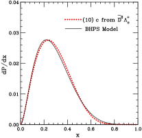
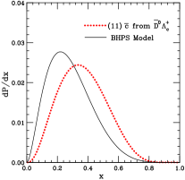
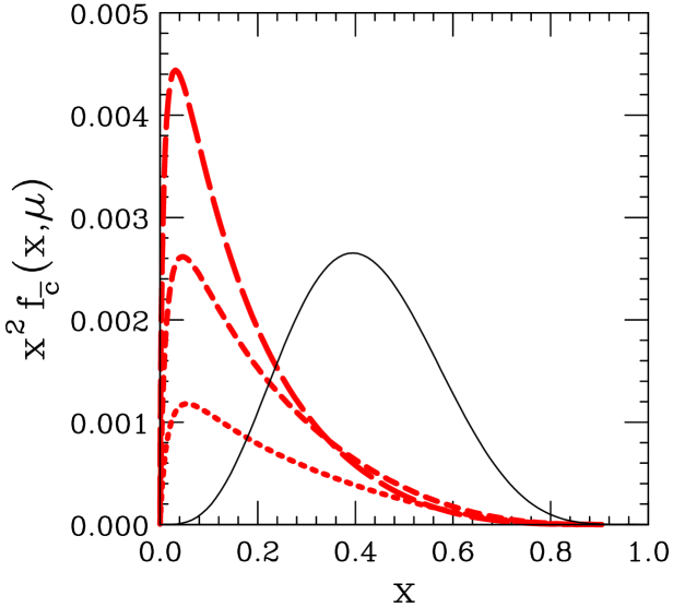
Figure 3 shows the $c$ distribution from $p\to\overline{D}^{0}\Lambda_{c}^{+}$. The result is very similar to the BHPS model. Figure 4 shows the $\bar{c}$ distribution from $p\to\overline{D}^{0}\Lambda_{c}^{+}$. On comparing Figs. 3 and 4, we once again find $\bar{c}(x)>c(x)$ at large $x$—for the same reason as described in footnote 1. This was observed previously in a meson cloud model that is rather similar to this one [11]. It is opposite to the asymmetry predicted by [15].

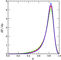
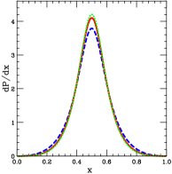
A contribution from the two-body state $p\,J\!/\!\psi$ is also possible. It is even slightly favored over $\overline{D}^{0}\Lambda_{c}^{+}$ by having a lower threshold mass: $m_{p}+m_{J\!/\!\psi}=4.035\,\mathrm{GeV}<m_{D}+m_{\Lambda_{c}}=4.149\,\mathrm{GeV}$. (This is in contrast to the SU(4)-analog case of strangeness, where $K^{+}\Lambda^{0}$ is strongly favored over $p\,\phi^{0}$ by $m_{K^{+}}+m_{\Lambda^{0}}=1.609\,\mathrm{GeV}\ll m_{p}+m_{\phi}=1.958\,\mathrm{GeV}$.) Figure 5 shows the $c=\bar{c}$ distribution from the model of a $p\,J\!/\!\psi$ Fock space component and the model of $c$ or $\bar{c}$ in $J\!/\!\psi$. A range of reasonable parameters for the suppression of large masses was tried and all give similar results.

Figure 6: Fraction of proton momentum carried by valence quarks, gluon, $b+\bar{b}$, and $c+\bar{c}$ as a function of scale $\mu$, with uncertainty bands. The $b+\bar{b}$ and $c+\bar{c}$ curves were multiplied by $10$ for clarity. The dot-dash line indicates the level of intrinsic $c+\bar{c}$ predicted by BHPS, also multiplied by $10$.

Figure 7: Distribution $x^{2}f_{\bar{c}}(x)$ from CTEQ6.1 (extrinsic charm) at $\mu=2$, $5$, $100\,\mathrm{GeV}$ (short, medium, long dash) compared to BHPS model (intrinsic charm) (solid). The intrinsic charm component dominates at large $x$.

4 Comparison with perturbative ${\mathbf{c\bar{c}}}$ and ${\mathbf{b\bar{b}}}$

When normalized to $1\%$ probability, the BHPS model predicts that a fraction $\int_{0}^{1}[f_{c}(x)+f_{\bar{c}}(x)]\,x\,dx=0.0057$ of the proton momentum is carried by nonperturbative charm. The models of Sections 2–3 give quite similar values, ranging from $0.0046$ to $0.0073\,$.

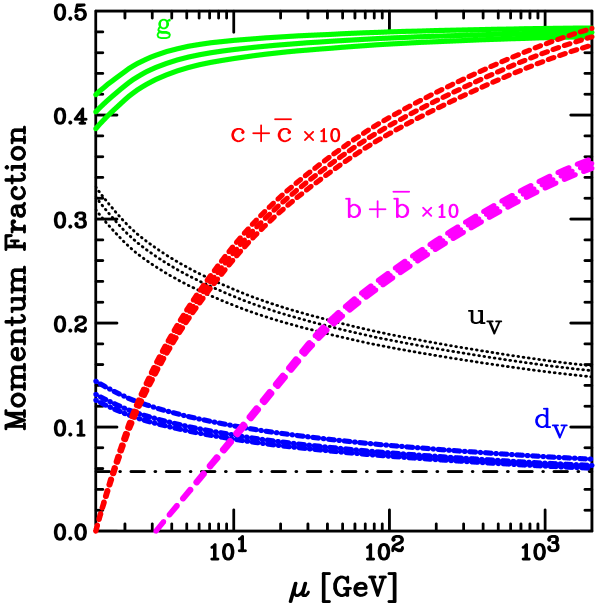
These possible intrinsic momentum fractions can be compared with the standard perturbative contributions to the proton momentum, which are shown in Fig. 6 as a function of $\mu$. (These were calculated from the CTEQ6.1 global analysis [2], with uncertainty ranges based on the eigenvector uncertainty sets [16, 2].) Note that the $c+\bar{c}$ and $b+\bar{b}$ fractions have been multiplied by 10 for clarity. We see that a possible $1\%$ intrinsic charm contribution would be rapidly overtaken by perturbatively generated charm, once the evolution in $\mu$ has proceeded a short distance above $m_{c}$. Gluon splitting similarly generates $b\bar{b}$ pairs rapidly above the scale $\mu\!\sim\!m_{b}$. Thus intrinsic $c$ and $b$ cannot be expected to add significantly to the perturbatively generated $c$ and $b$ for most regions of $x$ and $\mu$.

Nevertheless, the intrinsic $c\bar{c}$ component may be very significant at large $x$. This is demonstrated by Fig. 7, which shows the probability distributions as a function of $x$, weighted by a factor $x^{2}$ to clarify the large-$x$ region. The intrinsic component is stronger than the perturbative one at $x>0.3$, even for $\mu$ as large as $100\,\mathrm{GeV}\,$. (The intrinsic component will of course also evolve with $\mu$, but that will not significantly alter this comparison.)

Figure 8: Parton distributions for $u$ (long dash), $d$ (short dash), $\bar{u}$ (long dash dot), $\bar{d}$ (short dash dot), and $g$ (dotted) at $\mu=2\,\mathrm{GeV}$, compared with $\bar{c}$ from the BHPS model (solid).

5 Comparison with light quarks and gluon

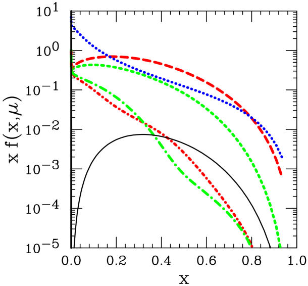
Figure 8 compares the BHPS model, which is representative of all the models described here, with the light-quark flavors and gluon from CTEQ6.1. It shows the remarkable result that with the assumption of $1\%$ intrinsic charm, the $c$ and $\bar{c}$ distributions are larger than $\bar{d}$ and $\bar{u}$ at large $x$. This result arises from the $m^{2}/x$ term in the off-shell distance of the heavy-quark states.

Figure 8 also shows that intrinsic $c$ and $\bar{c}$ are much smaller than the valence quark and gluon distributions. This implies that the possibility of IC does not significantly affect the light quark and gluon distributions. As a corollary, it negates a pretty speculation that IC could be the source of an unexpected feature of the CTEQ6.1 PDFs which can be seen in Fig. 8: the gluon distribution is larger than the valence quarks at very large $x$ for small $\mu$. (That feature is not a robust feature of the CTEQ PDFs, since it can be made to disappear by a small change in the gluon parameterization at $\mu_{0}$, with an insignificant increase ($\Delta\chi^{2}\approx 5$) in the $\chi^{2}\approx 2000$ of the global fit. The feature therefore does not actually require an explanation.)

6 Conclusion

Model	$A_{0}$	$A_{1}$	$A_{2}$
(1)	$520.517$	$4.611$	$11.477$
(2)	$0.904$	$1.271$	$5.703$
(3)	$0.179$	$0.496$	$4.164$
(4)	$0.785$	$1.220$	$5.519$
(5)	$0.401$	$0.886$	$4.908$
(6)	$0.187$	$0.521$	$4.194$
(7)	$0.387$	$0.822$	$5.017$
(8)	$0.374$	$1.010$	$4.422$
(9)	$0.473$	$0.994$	$4.986$
(10)	$2.238$	$1.897$	$6.095$
(11)	$2.245$	$2.511$	$4.929$
(12)	$591.400$	$5.065$	$10.708$
BHPS	$1.052$	$1.524$	$5.377$

Table 1: Coefficients for a simple parametrization of the models: $f_{c}(x)=dP/dx=A_{0}\,x^{A_{1}}\,(1-x)^{A_{2}}$. The normalization $A_{0}$ is chosen to make the momentum fraction $\int_{0}^{1}f_{c}(x)\,x\,dx$ or $\int_{0}^{1}f_{\bar{c}}(x)\,x\,dx$ equal to $1/350$, the value it has in the BHPS model.

The light cone ideas used here are at best qualitative and heuristic. It is not for example clear whether they should be applied in $\overline{\mathrm{MS}}$ or some other scheme; or at what scale $\mu_{0}$. They should nevertheless be a useful guide in the effort to measure intrinsic heavy flavors in the proton.

We have shown that intrinsic charm (IC) will provide the dominant contribution to $c$ and $\bar{c}$ at large $x$, if the shape of the IC distribution is given by the BHPS model and the normalization is anywhere near the estimated $1\%$ probability. All of the other light-cone based models we have examined have roughly the same shape in $x$ dependence, and hence they reinforce this result. Several of the models predict a difference between $c$ and $\bar{c}$, with $\bar{c}(x)-c(x)>0$ at large $x$. Similar conclusions for the shape apply for intrinsic $b$.

Assuming the $1\%$ probability is approximately correct for IC, $c$ is much smaller than $u$, $d$, and $g$ at all $x$, so it has no appreciable impact on the evolution of other flavors. Intrinsic $b$ is presumably even smaller.

An estimate of $(0.86\pm 0.60)\%$ was obtained for the IC probability some time ago [17, 18] by re-analysis of $F_{2}^{c}$ data in deep inelastic muon scattering on iron [19]. That estimate continues to be cited (see e.g. [5]) as evidence for the existence of IC, although it is obviously of limited statistical power; and when possible variations in the parton distributions are taken into account, the $F_{2}^{c}$ data are consistent with no IC [11, 21]. Measurements of $F_{2}^{c}$ at HERA [4] are also consistent with no IC, but those measurements are not at sufficiently large $x$ to have any sensitivity to it. For other experimental indications of IC, see [20].

In order to actually measure intrinsic charm or bottom, it will be necessary to have data that are directly sensitive to the large-$x$ component. Likely candidates are jet production with $c$- or $b$-tagging—either inclusively or in association with $W$, $Z$, or high-$p_{T}$ $\gamma$. It may also be possible to extract useful information from coherent diffractive dissociation processes such as $p\to p\,J\!/\!\psi$ on a nuclear target [22].

For convenience in future work, the model curves (1)–(12) that appear in Figs. 1–5 can be adequately represented by a simple parametrization which is given in Table 1. To create this table, the normalization coefficients $A_{0}$ were chosen to make the momentum fraction $\int_{0}^{1}f_{c}(x)\,x\,dx$ or $\int_{0}^{1}f_{\bar{c}}(x)\,x\,dx$ equal to $0.002857$, the value given by the BHPS model when that model is normalized to $1\%$ probability. This is different from the normalization of the curves shown in the Figs. 1–5, which was such that each curve corresponded to $1\%$ probability. This new normalization is more useful for applications, since it places more emphasis on large $x$, where intrinsic charm will be important if it is important at all. For comparison, the momentum carried by $s$ or $\bar{s}$ at $\mu=1.4\,\mathrm{GeV}$ is—as it should be—substantially larger (by a factor of $4$) than this working estimate of $0.002857$ for $c$ or $\bar{c}$.

Acknowledgements:

I thank Stan Brodsky for stimulating discussions. This research is supported by the National Science Foundation.

Appendix: Light-cone probability distributions from Feynman rules

This Appendix shows how to derive light-cone probability distributions directly from Feynman diagram rules by a thought experiment.

For simplicity, consider a spin 0 particle with mass $m_{0}$ that couples to spin 0 particles with masses $m_{1},\dots,m_{N}$ by a point coupling $ig$, as illustrated in Fig. 9(a). The thought experiment consists of scattering this system at very high energy from a target that interacts with only one of the constituents, as illustrated in Fig. 9(b). This target supplies an infinitesimal momentum transfer that puts the $N$-particle system on mass-shell (diffractive dissociation) with a cross section that must be proportional to the probability for that system in the original Fock space.

Figure 9: (a) Point coupling model; and (b) diffractive dissociation process used to compute its light-cone probability distribution.

Assume that the target provides a constant total cross section $\sigma_{0}$, with transverse momentum transfer dependence proportional to $\exp(-\beta\,\vec{q}_{\perp}^{\;2})$. The elastic differential cross section is

$${{d\sigma}\over{d\vec{q}_{\perp}^{\;2}}}={{\sigma_{0}^{\,2}}\over{16\pi}}e^{-\beta\,\vec{q}_{\perp}^{\;2}}$$ (12)

and hence the integrated elastic cross section is

$$\sigma_{\mathrm{el}}={{\sigma_{0}^{\,2}}\over{16\pi\beta}}\;.$$ (13)

By Feynman rules, Fig. 9(b) gives an amplitude

$${\mathcal{M}}={{2\,i\,g\,p_{N}\!\cdot\!q}\over{t-m_{N}^{\,2}}}\,\exp(-\beta\,{\vec{q}_{\perp}}^{\;2}/2)$$ (14)

and a cross section

$$d\sigma={{4\,\pi^{4}}\over{p_{0}\!\cdot\!q}}\,{{d^{3}q}\over{16\,\pi^{3}\,q^{(0)}}}\prod_{j=1}^{N}\!\left({{d^{3}p_{j}}\over{16\,\pi^{3}\,p_{j}^{(0)}}}\right)\delta^{(4)}(p_{0}+k-\sum_{j=1}^{N}p_{j}-q)\,|{\mathcal{M}}|^{2}\,.$$ (15)

Assume the gaussian parameter $\beta$ is large, corresponding to a large spatial extent of the target in impact parameter. We can then set $q_{\perp}=0$ everywhere except in the exponential factor and carry out the integral over $q_{\perp}$. The Fock space probability density $dP$ can be identified from the obvious relation

$$d\sigma=\sigma_{\mathrm{el}}\times dP\,.$$ (16)

Now introduce the light-cone components of all four-momenta, $p^{(\pm)}=(p^{(0)}\pm p^{(3)})/\sqrt{2}\,$, and define the light-cone momentum fractions $x_{j}=p_{j}^{(+)}/p_{0}^{(+)}$. The components $p_{0}^{(+)}$ and $q^{(-)}$ are taken to be large, with $p_{0\,\perp}=q_{\perp}=0$. The small components are determined by mass-shell conditions, e.g., $p^{2}=m^{2}$ $\Rightarrow$ $p^{(-)}=(p_{\perp}^{2}+m^{2})/(2p^{(+)})$. This leads to

$$dP={{1}\over{(16\,\pi^{3})^{N-1}}}\prod_{j=1}^{N}\!\left({{d^{2}p_{j{\scriptscriptstyle\perp}}\,dx_{j}}\over{x_{j}}}\right)\,\delta^{(2)}(\sum_{j=1}^{N}p_{j{\scriptscriptstyle\perp}})\,\delta(1-\sum_{j=1}^{N}x_{j})\,{{x_{N}^{\,2}\,g^{2}}\over{(t-m_{N}^{\,2})^{2}}}\;.$$ (17)

The covariant off-shell distance can be expressed conveniently in the form

$$m_{N}^{\,2}-t=m_{N}^{\,2}-\left(p_{0}-\sum_{j=1}^{N-1}p_{j}\right)^{\!2}=x_{N}\,(s-m_{0}^{\,2})\;,$$ (18)

where

$$s=\sum_{j=1}^{N}(p_{j{\scriptscriptstyle\perp}}^{\,2}+m_{j}^{\,2})/x_{j}\;.$$ (19)

This leads to the final result

$$dP={{1}\over{(16\,\pi^{3})^{N-1}}}\prod_{j=1}^{N}\!d^{2}p_{j{\scriptscriptstyle\perp}}\,\prod_{j=1}^{N}\!{{dx_{j}}\over{x_{j}}}\,\delta^{(2)}(\sum_{j=1}^{N}p_{j{\scriptscriptstyle\perp}})\,\delta(1-\sum_{j=1}^{N}x_{j})\,{{g^{2}}\over{(s-m_{0}^{\,2})^{2}}}$$ (20)

for the point-coupling model. Note that this result is completely symmetric in the particles $1,\dots,N$ as it should be—it does not depend on which particle was singled out to scatter in the thought experiment used to derive it. It is straightforward to include more complicated vertices and factors due to spin using this Feynman diagram approach. When that is done, the result can depend on which particle is assumed to scatter, but the ambiguity vanishes at the pole at $s=m_{0}^{\,2}$. Unitarity effects that keep the total probability equal to $1$ could also be included.

In this simple point-coupling model, high-mass Fock states are suppressed only by the “old-fashioned perturbation theory energy denominator” factor $(s-m_{0}^{\,2})^{-2}\,$. To make the model more realistic, there must be a further suppression of high mass states associated with wave function effects—if only to make the integrated probability finite. It is natural to suppose that the additional suppression is a function of $s$.

When a wave function factor $[F(s)]^{2}$ is included in Eq. (20), the transverse momentum integrals can be carried out by inserting the identity $1=\int\delta(\sum_{j}(p_{j{\scriptscriptstyle\perp}}^{\,2}+m_{j}^{\,2})/x_{j}-s)\,ds$, and then Fourier transforming this delta function and the transverse momentum conserving one. The result is

$$dP={{g^{2}}\over{(16\,\pi^{2})^{N-1}\,(N-2)!}}\prod_{j=1}^{N}\!dx_{j}\,\delta(1-\sum_{j=1}^{N}x_{j})\,\int_{s_{0}}^{\infty}{{(s-s_{0})^{N-2}\,[F(s)]^{2}\,ds}\over{(s-m_{0}^{\,2})^{2}}}$$ (21)

where $s_{0}=\sum_{j=1}^{N}m_{j}^{\,2}/x_{j}\,$. Note that $[F(s)]^{2}$ must go to zero faster than $1/s^{N-3}$ as $s\to\infty$ to make the integrated probability converge.

References

- [1] J. W. Negele et al., Nucl. Phys. Proc. Suppl. 128, 170 (2004) [hep-lat/0404005]; W. Schroers, Nucl. Phys. A 755, 333 (2005) [hep-ph/0501156].
- [2] J. Pumplin, D. R. Stump, J. Huston, H. L. Lai, P. Nadolsky and W. K. Tung, JHEP 0207, 012 (2002) [hep-ph/0201195]; D. Stump, J. Huston, J. Pumplin, W. K. Tung, H. L. Lai, S. Kuhlmann and J. F. Owens, JHEP 0310, 046 (2003) [hep-ph/0303013].
- [3] R. S. Thorne, A. D. Martin, W. J. Stirling and R. G. Roberts, [hep-ph/0407311].
- [4] A. Aktas et al. [H1 Collaboration], Eur. Phys. J. C 40, 349 (2005) [hep-ex/0411046]; A. Aktas et al. [H1 Collaboration], [hep-ex/0507081].
- [5] S. J. Brodsky, “Light-front QCD,” [hep-ph/0412101]; S. J. Brodsky, Few Body Syst. 36, 35 (2005) [hep-ph/0411056].
- [6] S. J. Brodsky, P. Hoyer, C. Peterson and N. Sakai, Phys. Lett. B 93, 451 (1980).
- [7] S. J. Brodsky, C. Peterson and N. Sakai, Phys. Rev. D 23, 2745 (1981); R. Vogt, Prog. Part. Nucl. Phys. 45, S105 (2000) [hep-ph/0011298]; T. Gutierrez and R. Vogt, Nucl. Phys. B 539, 189 (1999) [hep-ph/9808213]; G. Ingelman and M. Thunman, Z. Phys. C 73, 505 (1997) [hep-ph/9604289]; J. Alwall and G. Ingelman, Phys. Rev. D 71, 094015 (2005) [hep-ph/0503099]; J. Alwall, [hep-ph/0508126].
- [8] M. Franz, . V. Polyakov and K. Goeke, Phys. Rev. D 62, 074024 (2000) [hep-ph/0002240].
- [9] F. S. Navarra, M. Nielsen, C. A. A. Nunes and M. Teixeira, Phys. Rev. D 54, 842 (1996) [hep-ph/9504388]; S. Paiva, M. Nielsen, F. S. Navarra, F. O. Duraes and L. L. Barz, Mod. Phys. Lett. A 13, 2715 (1998) [hep-ph/9610310].
- [10] W. Melnitchouk and A. W. Thomas, Phys. Lett. B 414, 134 (1997) [hep-ph/9707387].
- [11] F. M. Steffens, W. Melnitchouk and A. W. Thomas, Eur. Phys. J. C 11, 673 (1999) [hep-ph/9903441].
- [12] A. I. Signal and A. W. Thomas, Phys. Lett. B 191, 205 (1987); W. Koepf, L. L. Frankfurt and M. Strikman, Phys. Rev. D 53, 2586 (1996) [hep-ph/9507218]; S. J. Brodsky and B. Q. Ma, Phys. Lett. B 381, 317 (1996) [hep-ph/9604393].
- [13] J. F. Donoghue and E. Golowich, Phys. Rev. D 15, 3421 (1977).
- [14] X. T. Song, Phys. Rev. D 65, 114022 (2002) [hep-ph/0111129].
- [15] S. J. Brodsky and B. Q. Ma, Phys. Lett. B 381, 317 (1996) [hep-ph/9604393].
- [16] J. Pumplin, D. R. Stump and W. K. Tung, Phys. Rev. D 65, 014011 (2002) [hep-ph/0008191].
- [17] E. Hoffmann and R. Moore, Z. Phys. C 20, 71 (1983).
- [18] B. W. Harris, J. Smith and R. Vogt, Nucl. Phys. B 461, 181 (1996) [hep-ph/9508403].
- [19] J. J. Aubert et al. [European Muon Collaboration], Nucl. Phys. B 213, 31 (1983).
- [20] R. Vogt, S. J. Brodsky and P. Hoyer, Nucl. Phys. B 360, 67 (1991); R. Vogt, S. J. Brodsky and P. Hoyer, Nucl. Phys. B 383, 643 (1992); R. Vogt and S. J. Brodsky, Phys. Lett. B 349, 569 (1995) [hep-ph/9503206]; R. Vogt and S. J. Brodsky, Nucl. Phys. B 478, 311 (1996) [hep-ph/9512300].
- [21] A. D. Martin, R. G. Roberts, W. J. Stirling and R. S. Thorne, Eur. Phys. J. C 4, 463 (1998) [hep-ph/9803445]; M. Gluck, E. Reya and A. Vogt, Eur. Phys. J. C 5, 461 (1998) [hep-ph/9806404].
- [22] J. Badier et al. [NA3 Collaboration], Z. Phys. C 20, 101 (1983); S. J. Brodsky and P. Hoyer, Phys. Rev. Lett. 63, 1566 (1989).
- [23] A. I. Signal, A. W. Schreiber and A. W. Thomas, Mod. Phys. Lett. A 6, 271 (1991); S. Kumano, Phys. Rev. D 43, 59 (1991); S. Kumano, Phys. Rev. D 43, 3067 (1991).
- [24] W. Melnitchouk, J. Speth and A. W. Thomas, Phys. Rev. D 59, 014033 (1999) [hep-ph/9806255].