2005 International Linear Collider Workshop - Stanford, U.S.A.
New Physics at the TeV Scale and Precision Electroweak Studies

Abstract

In this summary we review some recent developments in New Physics at the TeV scale. We concentrate on measurements at the ILC that can distinguish between some of the models that have recently been discussed, concentrating on results presented at this workshop: The Little Higgs Model, models of Large Extra Dimensions; Randall-Sundrum (RS), Arkani-Hamed Dimopoulos Dvali (ADD), and Universal Extra Dimensions (UED). Some recent results on constraining effective Lagrangian parametrizations of new physics are also presented.

I INTRODUCTION

There is a universal consensus that the standard model is a low energy effective theory and that some form of new physics exists beyond the standard model (BSM). The literature is full of candidate theories but it will be experiment that shows the way. This contribution reviews some of the recent developments in BSM phenomenology with an emphasis on results presented in the BSM working group sessions. However, it would be a mistake to consider this topic in isolation from the other working group topics. I expect the next few years to be exciting times in particle physics with the start of the LHC leading to major advances in our understanding of electroweak symmetry breaking. It is likely that this will give us the first hints of physics BSM but it is possible that the first hints will come from elsewhere, perhaps anomalous properties of the top quark. Maybe this new physics is supersymmetry. And maybe the new physics unravelled at the ILC will explain some of the puzzles in cosmology. The point is that while the physics topics have been divided up into EWSB, SUSY, Top/QCD, New Physics, and Cosmology, they are all connected and one should not forget this when focusing on individual topics. This will be apparent in some of the examples chosen to describe the search for new physics.

There are numerous models of new physics. An important task of the ILC will be to disentangle the possibilities and identify the correct one. We start with a very brief overview of some of the possibilities, focusing on models of recent interest. In the remainder of this summary I will examine some of approaches discussed to understand the underlying physics. This summary should not by any means be viewed as a comprehensive overview; it is a snapshot of a selection of topics covered at this workshop and studied over the last few years. More detailed reviews are given by LHC/LC working group in Ref. Weiglein:2004hn . See also Ref. Dawson:2004xz ; Moortgat-Pick:2005cw ; Lykken:2005up . An important omission in this summary is the subject of Higgless Elecroweak Symmetry Breaking. A selection of recent papers on this subject is given in Ref. Csaki:2003zu

II MODELS OF NEW PHYSICS

There are many models of new physics. Some of the models that have attracted attention recently are the Little Higgs model Arkani-Hamed:2002qy , various models of extra dimensions Antoniadis:1990ew ; Rizzo:2004kr ; ADD Arkani-Hamed:1998nn , RS Randall:1999ee , UED Appelquist:2000nn , and the Higgsless model Csaki:2003zu . However, we shouldn’t ignore older models that, although less fashionable, may contain elements of truth in them. Some models of continued interest are extended gauge sectors with extra $U(1)$ factors Leike:1998wr like the $E_{6}\to SU(5)\times U(1)_{\chi}\times U(1)_{\psi}$ where the extra $U(1)$ factors give rise to extra neutral gauge bosons, the left-right symmetric model, $SU(2)_{L}\times SU(2)_{R}\times U(1)$, and dynamical symmetry breaking models such as technicolour and topcolour Hill:2002ap . From the point of view of disentangling these possibilities we need to understand what they have in common and how we can distinguish them. As a result I will focus on predictions of the various models and how we can unravel the underlying physics rather than on theoretical details of the various models.

In the next few paragraphs I will give a rather superficial survey of some recent models and refer the interested reader to the literature. My purpose here is to simply identify the characteristics of the various models that might reveal themselves by experiment.

Little Higgs Models

Arkani-Hamed:2002qy are a new approach to stabilize the weak scale against radiative corrections. They predict new gauge bosons $W_{H}^{\pm}$, $Z_{H}$, and $B_{H}$ and a new heavy top quark at the TeV scale. The parameters of the Littlest Higgs model relevant to the discussion are $f$, the vev that breaks the global symmetry group to a smaller group and sets the mass scale of the new heavy particles in the model, and gauge boson mixing angles $s$ and $s^{\prime}$. A light Higgs boson is expected at ${\cal O}(100)$ GeV. The couplings to $\gamma\gamma$ are sensitive to new physics running in the loop so measurement of the Higgs $\gamma\gamma$ and $gg$ BR’s is a sensitive test of the heavy top quark, extra gauge bosons and new scalar particles expected in Little Higgs models. Other modifications are expected due to mixing of TeV-scale particles with SM particles and corrections to SM parameters.

Extra Dimensions

Rizzo:2004kr In most scenarios our 3-dimensional space is a 3-brane embedded in a $D$-dimensional spacetime. The basic signal is a Kaluza Klein (KK) tower of states corresponding to a particle propagating in the higher dimensional space-time. The details depend on the geometry of the extra dimensions with many different variations.

• The ADD scenario Arkani-Hamed:1998nn has a KK tower of graviton states in 4 dimensions that behaves like a continuous spectrum which Hewett Hewett:1998sn parametrized as the effective operator

  $$i{{4\lambda}\over{M_{H}^{4}}}T^{\mu\nu}T_{\mu\nu}$$ (1)

  that will lead to deviations in $e^{+}e^{-}\to f\bar{f}$ dependent on $\lambda$ and $M_{H}$, a cut-off scale on the summation over the KK states. ADD also predicts graviscalars and gravitensors propagating in extra dimensions. The parameters of interest for ADD are the mixing between the Higgs boson and the graviscalar, $\xi$, the number of extra dimensions, $\delta$, and the $M_{D}$ scale. The Mixing of the graviscalar with the Higgs boson leads to a significant invisible width of the Higgs.

• In the Randall Sundrum Model Randall:1999ee 2 3+1 dimensional branes are separated by a 5th dimension. It predicts the existence of a radion which corresponds to fluctuations in the size of the extra dimension. Radions have anomalous couplings with gluon and photon pairs and since they can mix with the Higgs boson this alters the corresponding Higgs BR’s. In the RS model the KK graviton spectrum is discrete and unevenly spaced. It is described in terms of two parameters, the mass of the first KK state and the coupling strength of the graviton. TeV scale graviton resonances are expected to be produced in 2-fermion channels.

• In the Universal Extra Dimension scenario Appelquist:2000nn all SM particles propagate in the bulk resulting in KK towers for the SM particles with spin quantum numbers identical to SM particles. The resulting spectrum resembles that of SUSY and the conservation of KK number at tree level ensures that the lightest KK partner is stable and is always pair produced so that the signatures look alot like signatures of SUSY.

• An extension to both ADD and RS is the existence of higher curvature terms in the action for gravity that may manifest themselves as we approach $M_{pl}\sim 1$ TeV Rizzo:2005xr . In RS the dominant effect is a modification of the KK graviton mass spectrum and their couplings to matter. In the case of ADD the modifications are quite different. The usual ADD signatures remain unaltered but the modifications lead to the production of long lived black holes. Both the RS and ADD modifications can be studied at the ILC.

To summarize, the models predict extra Higgs bosons (doublets and triplets), radions, graviscalars, gravitons, KK excitations of the $\gamma$, $Z$, $W$, extra gauge bosons and extra fermions. Almost all of the models predict new $s$-channel structures at the TeV scale, either as extended gauge bosons or new resonances. To sort out the models we first need to elucidate and complete the TeV particle spectrum and to then make precision measurements of their properties.

III PRECISION ELECTROWEAK MEASUREMENTS

There are several paths to discovering new physics. The most straight forward is the direct discovery of new particles. The next possibility is the indirect discovery by comparing deviations from the SM to specific new models. The final approach is to test for new physics by measuring the parameters of effective Lagrangians.

A starting point for indirect searches for new physics is to consider the common features of the various models. In almost all cases a new $s$-channel structure is expected at the TeV scale either in the form of extra gauge bosons or as some other type of new resonance. Each of these models predicts different properties for these new resonances so to distinguish between the possibilities we will need to make precision measurements. While it is likely that discoveries at the LHC will get us started it is almost a certainty that we will need the ILC to discriminate between models. An incomplete list of tools we will have at the ILC are measurements of the various di-fermion channels, anomalous fermion couplings, anomalous gauge boson couplings and measurement of the Higgs couplings.

Let’s start by considering the possibility that the LHC discovers an $s$-channel resonance in the dilepton invariant mass distribution. There are numerous possibilities of what it might be; graviton, KK excitations, a $Z^{\prime}$, etc. The LHC can give some information about what it might be using the invariant mass distribution and forward backward asymmetry measurements Rizzo:2003ug ; Davoudiasl:2000wi ; Dittmar:2003ir . However, these measurements are rather crude and would require significant luminosity to achieve any sort of precision and resolving power. On the other hand if we assume the LHC discovers a single, rather heavy resonance, the ILC can make many precision measurements such as cross section and widths (depending on the mass for the latter case), angular distributions, and its couplings via decays and polarization measurements.

If the resonance is below the ILC threshould it can be produced on resonance. In this case angular distributions can be tested against different spin hypothesis to distinguish between a spin 2 graviton and say, a spin 1 $Z^{\prime}$. BR’s could be used to measure the resonance couplings which would distinguish between the universal couplings of a graviton or the unique couplings expected for the various $Z^{\prime}$ scenarios. Angular distributions and branching ratios for spin-2 gravitons from Davoudiasl, Hewett and Rizzo Davoudiasl:2000wi are shown in Fig. 1.

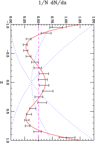
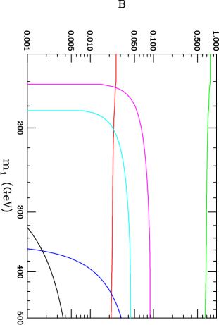
Figure 1: Left side: Normalized angular distribution ($z=\cos\theta$) for the decay of a spin-2 graviton into fermion pairs (the ‘w’-shaped curve) in comparison to similar decays by either spin-0 (dashed) or spin-1 (dotted) particles. The data with errors show the result from a typical sample of 1000 events. Right side: Mass dependencies of the two-body branching fractions for the first graviton KK state in the case where the SM fields are on the wall. From top to bottom on the right side of the figure the curves are for dijets, $W$’s, $Z$’s, tops, dileptons and Higgs pairs assuming a Higgs mass of 120 GeV. From Davoudiasl, Hewett and Rizzo Davoudiasl:2000wi .

III.1 Precision Measurements Using Di-Fermion Channels

A more likely scenario is that the mass of a new state is beyond the direct reach of the ILC. In this case we can still learn a considerable amount about a new resonance. There are numerous di-fermion channels and since the couplings to each channel is model dependent, observables such as cross sections to specific final states, forward-backward asymmetries, and left-right asymmetries can be used to distinguish between models.

A first step is to disentangle the spin of the exchange particle. As a concrete example there have been a number of studies examining how to distinguish virtual graviton KK expected in the ADD scenario of finite size extra dimensions from other possibilities. Hewett Hewett:1998sn parametrized the exchange of virtual graviton KK states as the effective operator given in Eqn. 1. She showed how interference with SM amplitudes leads to deviations in the dilepton observables dependent on both $\lambda$ and $M_{H}$. Rizzo has studied how multipole moments could be used to distinguish spin 2 from spin 1 Rizzo:2002pc . Osland Pankov and Paver used the various difermion observables to estimate to what extent $M_{H}$ could be constrained at the ILC Osland:2005ee ; Osland:2003fn . More recently they constructed a “Forward-Backward Centre-Edge” defined as $\sigma_{CE,FB}=\sigma_{C,FB}-\sigma_{E,FB}$ to identify graviton exchange and act as a discriminator between possible models Pankov:2005qi ; Pankov:2005ar . In this defination “centre” refers to a region with $|\cos\theta|\leq Z^{*}$ and “edge” refers to $|\cos\theta|>Z^{*}$ with $z^{*}$ a value that can be varied to optimize the discrimination power and $FB$ is the forward-backward asymmetry evaluated for the centre region and the edge region. $A_{CEFB}$ is shown in Fig. 2 for a contact interaction and ADD graviton exchange. They estimated that the ILC would be sensitive to $M_{H}$ up to 3.5 and 5.8 TeV for $\sqrt{s}=0.5$ and 1.0 TeV respectively with ${\cal L}_{int}=500$ fb^-1.

Figure 2: $\Delta A_{\rm CE,FB}(z^{*})$ in the CI and the ADD scenarios for the indicated values of $\Lambda$ and $M_{H}$. The $\pm$ superscripts refer to positive and negative interference, respectively. The vertical bars represent the statistical uncertainty at a LC with $\sqrt{s}=0.5$ TeV and ${\cal L}_{\rm int}=50\,fb^{-1}$. From Osland Pankov and Paver Pankov:2005qi ; Pankov:2005ar

A next step would be to measure the resonance couplings. Riemann used the leptonic observables to demonstrate that one can extract a $Z^{\prime}$ couplings and discriminate between models Aguilar-Saavedra:2001rg . A more recent analysis is shown in Fig. 3 which shows the resolution power for $Z^{\prime}$’s coming from the $E_{6}$ $\chi$, LR-symmetric, Littlest Higgs, and KK excitations. Note that the couplings shown for the KK case do not in fact correspond to the KK $Z^{\prime}$ couplings as in this model there are both photon and $Z$ KK excitations. The point is simply the KK model can be distinguished from other models. These figures were produced for $\sqrt{s}=500$ GeV and ${\cal L}_{int}=1$ab^-1 assuming electron and positron polarization of 80% and 60% respectively, $\Delta P_{e^{\pm}}=0.5\%$, $\Delta{\cal L}=0.5\%$, and $\Delta^{sys}\epsilon_{lepton}=0.25\%$. There is a two-fold ambiguity in the signs of the lepton couplings since all lepton observables are bilinear products of the couplings. The hadronic observables can be used to resolve this ambiguity since for this case the the quark and lepton couplings enter the interference terms linearly.

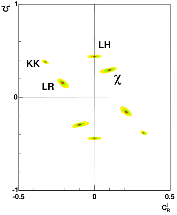
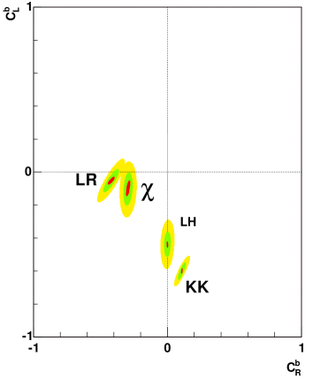
Figure 3: Resolving power (95% CL) for $M_{Z^{\prime}}=1$, 1.5, and 2 TeV and $\sqrt{s}=500$ GeV, ${\cal L}_{int}=1$ab^-1. The left side is for leptonic couplings based on the leptonic observables $\sigma$, $A_{LR}$, $A_{FB}$. The right side is for $b$ couplings based on $b$ observables $\sigma$, $A_{FB}$, $A_{FB}(pol)$ assuming that the leptonic couplings are known and a $b$-tagging efficiency of 70%. The couplings correspond to the $E_{6}$ $\chi$, LR, LH, and KK models. From Ref. godfrey .

A complementary approach was described by Conley Le and Hewett Conley:2005et who showed how the Little Higgs parameter space can be probed in the di-fermion channels. Their results are shown in Fig. 4 which indicates how well the parameters of the model can be constrained assuming that the mass of the $Z_{H}$ is known from the LHC.

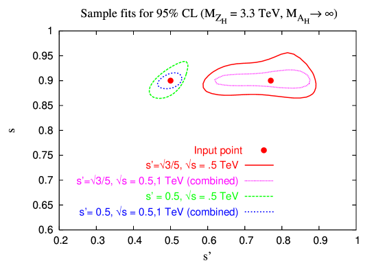
Figure 4: 95% CL sample fits to the data points ($s=0.9$, $s^{\prime}=0.5$) and ($s=0.9$, $s^{\prime}=\sqrt{3/5}$) using $e^{+}e^{-}\to f\bar{f}$ observables at a 500 GeV ILC, taking $M_{Z_{H}}=3.3$ TeV and $M_{A_{H}}\rightarrow\infty$. Also shown for each point is an improved fit from adding data from a $\sqrt{s}=1$ TeV, ${\cal L}=500\hbox{fb}^{-1}$ run at the ILC. From Conley, Le, and Hewett Conley:2005et .

The di-fermion channel has also been applied to other possible new physics. Riemann studied the sensitivity to the UED model level 2 KK $Z$ excitations in the di-fermion channels Riemann:2005es . Due to KK number conservation the KK excitations only couple to conventional fermions through loops. As a result the couplings are much smaller than SM couplings and $\sigma(e^{+}e^{-}\to f\bar{f})$ is much less sensitive to UED KK excitations than to other types of new gauge bosons.

A final example is that of Universal Extra Dimensions (UED). The KK spectrum in UED closely resembles that of SUSY. The typical signal for SUSY is missing $\not{E}_{T}$. So, for example, if a signal with significant $\not{E}_{T}$ was observed at the LHC it is quite possible that one could not decide if it was due to SUSY or UED Battaglia:2005zf ; Battaglia:2005ma . However the spins of SUSY particles are different than that of UED KK particles. One can take advantage of this by studying the angular distributions of the outgoing muons in $e^{+}e^{-}\to\mu^{+}\mu^{-}+\not{E}_{T}$. In UED this signature arises from KK muon production, $e^{+}e^{-}\to\mu_{1}^{+}\mu_{1}^{-}\to\mu^{+}\mu^{-}\gamma_{1}\gamma_{1}$ while in SUSY it arises from smuon pair production, $e^{+}e^{-}\to\tilde{\mu}^{+}\tilde{\mu}^{-}\to\mu^{+}\mu^{-}\tilde{\chi}_{1}^{0}\tilde{\chi}_{1}^{0}$. For UED the resulting muon angular distribution goes like $1+\cos^{2}\theta$ while for SUSY it goes like $1-\cos^{2}\theta$. The ISR-corrected theoretical predictions for the angular distributions for UED and SUSY are shown in Fig. 5. Clearly, the two cases can be discriminated. In addition to angular distributions threshold scans and energy distributions can also be used as discriminators of UED and SUSY Battaglia:2005zf ; Battaglia:2005ma . In particular, the threshold cross section for $e^{+}e^{-}\to\mu^{+}\mu^{-}+\not{E}_{T}$ goes like $\beta^{3}$ $(\beta=\sqrt{1-M^{2}/E^{2}_{beam}})$ in the MSSM and like $\beta$ in UED Battaglia:2005zf ; Battaglia:2005ma .

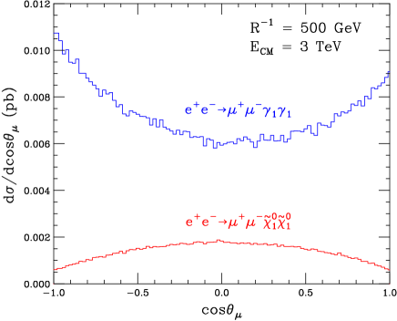
Figure 5: Differential cross-section $d\sigma/d\cos\theta_{\mu}$ for UED (blue, top) and supersymmetry (red, bottom) as a function of the muon scattering angle $\theta_{\mu}$. From Battaglia, Datta, De Roeck, Kong and Matchev Battaglia:2005ma .

As an aside one should not forget the considerable experimental effort that goes into these measurements. For example, $b$-tagging is an extremely powerful tool for ID’ing models so the understanding $b$-purity versus efficiency is an important issue to understand. Studies of this and other vertex detector issues were presented by Hillert. Luminosity and beam parameter measurements was another important issue described by Ingbir and Torrence.

III.2 Precision Measurement of Higgs Boson Properties

In addition to measurements of difermion observables, precision measurements of Higgs properties can be another important discriminator of models. Higgs properties have been studied in a wide variety of models using many different processes. In a first example Lillie studied Higgs properties in the Randall Sundrum model (RS) Lillie:2005pt . In this model, Higgs production is enhanced at the LHC and in $\gamma\gamma$ collisions but reduced at the ILC. A probably more distinctive signal is that Higgs decays are substantially modified from their SM values.

Battaglia et al studied ADD at the ILC Battaglia:2004js . Mixing of the SM Higgs with the graviscalar induces an invisible width compared to direct SM decay. The ILC can measure this invisible width directly and using $HZ$ production. The invisible width can be deduced in the $HZ$ process by observing the $Z$ boson and reconstructing the missing energy recoiling against it. The number of extra dimensions can be constrained by measuring the $e^{+}e^{-}\to\gamma+\not{E}$ at different values of $\sqrt{s}$ Weiglein:2004hn . Combined with a Higgs mass measurement from the LHC can constrain the ADD parameter space.

Precision measurements of the Higgs partial widths are a another powerful tool for distinguishing models. The two-photon and two-gluon partial widths are modified by heavy particles running in the loop and by shifts to the SM $W$-boson and $t$-quark masses Han:2003gf . Fig. 6 shows the range of $\Gamma(H\to gg)$ versus $\Gamma(H\to\gamma\gamma)$ normalized to the SM values for different Higgs masses and values of the decay constant parameter of the Little Higgs model Han:2003gf . It is clear that precision measurements of the BR’s offers a good means of constraining the parameters of this model.

Figure 6: Range of values of $\Gamma(H\to\gamma\gamma)$ accessible in the LH model as a function of $f$, normalized to the SM value, for $m_{H}=120$, 150 and 180 GeV and $f=1$, 2, and 3 TeV. From Han, Logan, McElrath and Wang Han:2003gf .

Conley Le and Hewett also studied the process $e^{+}e^{-}\to Zh$ in the Little Higgs model Conley:2005et . One of the hallmarks of Little Higgs models is the coupling of heavy gauge bosons to $Zh$. Thus, a signature of the Little Higgs model is deviations from the SM in $\sigma(e^{+}e^{-}\to Zh)$. The sensitivity of this process to the parameters of the model are shown in Fig. 7 for $\sqrt{s}=500$ GeV and assuming ${\cal L}_{int}=500$ fb^-1 which gives $\delta\sigma_{Zh}/\sigma_{Zh}=1.5\%$. The $\sigma(e^{+}e^{-}\to Zh)$ measurement covers a large region of the parameter space but there are still large regions to explore so perhaps other observables might be useful. In any case the $\sigma(e^{+}e^{-}\to Zh)$ measurements would be a useful complement to the difermion measurements in some regions of the LH parameter space and would provide a confirmation of this hallmark feature of the LH model.

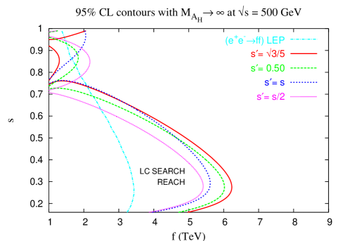
Figure 7: The ILC search reach from the process $e^{+}e^{-}\rightarrow Z_{L}h$ for various values of $s^{\prime}$, taking $\sqrt{s}=500$ and $M_{A_{H}}\rightarrow\infty$. The LEP II exclusion region from $e^{+}e^{-}\rightarrow f\bar{f}$ is shown for $s^{\prime}=s/2$ for comparison. From Conley, Le, and Hewett Conley:2005et .

IV PRECISION MEASUREMENTS AND EFFECTIVE LAGRANGIANS

In the examples given so far we assumed specific models and examined how well precisions measurements could either detect them or discriminate them from other models. A more general approach is to use the language of effective Lagrangians Krstonosic:2005qp ; Kilian:2005bz ; Osland:2005ee . Generically ${\cal L}_{eff}$ can be written:

$${\cal L}_{eff}={\cal L}_{SM}+\sum_{i}{{c_{i}}\over{\Lambda^{p}}}{\cal O}^{(4+p)}$$ (2)

where $\Lambda$ reflects the scale of new physics and the details of the new physics (couplings, chiral structure etc.) are parametrized in the coefficients $c_{i}$. For example, new interactions such as $s$-channel $Z^{\prime}$’ or $t$-channel leptoquark exchange can be parametrized as 4-fermion interactions if $\sqrt{s}<<\Lambda$.

In the gauge sector the trilinear gauge boson vertex $\gamma WW$ can be sensitive to new physics via new particles included in the vertex loop corrections Monig:2005ge . It has become the practice to parametrize the trilinear gauge boson vertices in terms of $k_{\gamma}$ and $\lambda_{\gamma}$. Mönig and Sekaric presented results of a detailed simulation including polarization and backgrounds of $\gamma\gamma\to W^{+}W^{-}\to q\bar{q}q\bar{q}$ at $\sqrt{s}_{ee}=500$ GeV Monig:2005ge . Their results on $k_{\gamma}$ and $\lambda_{\gamma}$ sensitivities comparing $e^{+}e^{-}$, $e\gamma$ and $\gamma\gamma$ modes for $\sqrt{s}_{ee}=500$ GeV and ${\cal L}_{int}=1000$ fb^-1 are shown in Table 1.

Table 1: Comparison of the $\kappa_{\gamma}$ and $\lambda_{\gamma}$ sensitivities at $\gamma e$-, $\gamma\gamma$- and $e^{+}e^{-}$-colliders estimated at $\sqrt{s_{ee}}=500$ GeV using the polarised beams. In case of photon colliders, the background and the pileup are included. (^∗) denotes the estimation at the generator level.

	$\sqrt{s_{ee}}=500$ GeV
LEFT	$\gamma e$	$\gamma\gamma$		$e^{+}e^{-}$
Mode	Real/Parasitic $|J_{Z}|=3/2$	$|J_{Z}|=2$	$J_{Z}=0$	$|J_{Z}|=1$
$\int{\cal L}\Delta t$	160 fb-1/230 fb-1	1000 fb-1		500 fb-1
${{\Delta}L}$	0.1$\%$	0.1$\%$	1$\%$	-
${\Delta}{\kappa}_{\gamma}{\cdot}10^{-4}$	10.0/11.0	7.0	27.8	3.6∗
${\Delta}{\lambda}_{\gamma}{\cdot}10^{-4}$	4.9/6.7	4.8	5.7	11.0∗

A strongly interacting weak sector would manifest itself in weak boson scattering, in particular in the quartic couplings. In the chiral Lagrangian parametrization one operator of interest is (for other operators not shown see for example Ref. Krstonosic:2005qp ; Kilian:2005bz ):

$${\cal L}_{4}={{\alpha_{4}}\over{16\pi^{2}}}Tr(V_{\mu}V_{\nu})\;Tr(V^{\mu}V^{\nu})$$ (3)

Again, one can calculate the values of these coefficients for specific models so that the the values and patterns of the coefficients $\alpha_{i}$ will codify the underlying new physics. Precision measurements of these coefficients will be needed to disentangle the underlying physics. The quartic vertices can be studied in numerous gauge boson scattering processes such as $e^{+}e^{-}\to\nu\bar{\nu}W^{+}W^{-}$ but also in triboson production processes such as $e^{+}e^{-}\to W^{+}W^{-}Z$. An important goal is to produce a full and consistent set of limits using all possible processes. Once this is done one can produce a strategy of measurements to constrain various models of new physics. To this end Krstonosic Krstonosic:2005qp presented results of a new analysis of gauge boson scattering and triple gauge boson production. Their results are summarized in Fig. 8. To obtain these bounds on $\alpha_{4}$ and $\alpha_{5}$ they assumed the same integrated luminosity and $80\%$ left $e^{-}$ and $40\%$ right $e^{+}$ polarization for scattering and $80\%$ right $e^{+}$ and $60\%$ left $e^{-}$ polarization for triple production. The same luminosity based conclusion was made after comparison of $e^{+}e^{-}$ and $e^{-}e^{-}$ running modes leaving the experimental physicist several ways to achieve the desired precision.

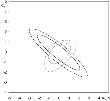
Figure 8: Comparison of estimated sensitivities for $\alpha_{4}$ and $\alpha_{5}$ at $\sqrt{s}=1000$GeV from weak boson scattering (black) and triple boson production (gray). Lines represent $68\%$ (full) and $90\%$ (dashed) confidence level contours. From Krstonosic, Mönig, Beyer, Schmidt, and Schröder Krstonosic:2005qp .

V CONCLUSIONS

The ILC is an instrument for making precision measurements. These are needed to disentangle the underlying new physics that may be hinted at or unearthed elswhere. For example, if an $s$-channel resonance were discovered at the LHC, the ILC would be needed to make precision measurements of its properties. Without these measurements, complementary to those of the LHC, it will be unlikely we will know the underlying theory. Another example is the discovery of a light Higgs boson at the LHC. Again, precision measurements at the ILC are needed to determine its origins. Some recent examples that have been discussed in the literature and presented at this workshop are distinguishing between a SM Higgs, SUSY, ADD, etc. These examples take advantage of a prior discovery at the LHC to extract further information using precision measurements at the ILC. There are other examples for which the ILC has a higher reach than the LHC via indirect effects such as interference of new interactions with the SM or via loop contributions to effective interactions.

An important task for our community is to continue to strengthen the case that the ILC is needed, especially in the era of the LHC. To do this we shouldn’t forget the LHC. Working on LHC physics is needed to understand its strengths and weaknesses thereby pointing out where the ILC can contribute crucial measurements. The rewards of our efforts might be in a press release by the ILC Director proclaiming “This result will send theorists back to their drawing boards”, and what could be more exciting than that!

- (1) G. Weiglein et al. [LHC/LC Study Group], hep-ph/0410364.
- (2) S. Dawson and M. Oreglia, Ann. Rev. Nucl. Part. Sci. 54, 269 (2004) [hep-ph/0403015].
- (3) G. Moortgat-Pick et al., hep-ph/0507011.
- (4) J. D. Lykken, hep-ph/0503148.
- (5) C. Csaki, C. Grojean, L. Pilo and J. Terning, Phys. Rev. Lett. 92, 101802 (2004) [hep-ph/0308038]; C. Csaki, C. Grojean, H. Murayama, L. Pilo and J. Terning, Phys. Rev. D 69, 055006 (2004) [hep-ph/0305237]; C. Csaki, hep-ph/0412339; T. G. Rizzo, hep-ph/0405094; H. Davoudiasl, J. L. Hewett, B. Lillie and T. G. Rizzo, Phys. Rev. D 70, 015006 (2004) [hep-ph/0312193]; A. Birkedal, K. Matchev and M. Perelstein, Phys. Rev. Lett. 94, 191803 (2005) [hep-ph/0412278].
- (6) N. Arkani-Hamed, A. G. Cohen, E. Katz and A. E. Nelson, JHEP 0207, 034 (2002) [hep-ph/0206021].
- (7) I. Antoniadis, Phys. Lett. B 246, 377 (1990).
- (8) Recent pedagogical introductions to extra dimensions are given by T. G. Rizzo, eConf C040802, L013 (2004) [hep-ph/0409309] and K. Cheung, hep-ph/0409028.
- (9) N. Arkani-Hamed, S. Dimopoulos and G. R. Dvali, Phys. Rev. D 59, 086004 (1999) [hep-ph/9807344]. N. Arkani-Hamed, S. Dimopoulos and G. R. Dvali, Phys. Lett. B 429, 263 (1998) [hep-ph/9803315]. I. Antoniadis, N. Arkani-Hamed, S. Dimopoulos and G. R. Dvali, Phys. Lett. B 436, 257 (1998) [hep-ph/9804398].
- (10) L. Randall and R. Sundrum, Phys. Rev. Lett. 83, 3370 (1999) [hep-ph/9905221].
- (11) T. Appelquist, H. C. Cheng and B. A. Dobrescu, Phys. Rev. D 64, 035002 (2001) [hep-ph/0012100]; H. C. Cheng, K. T. Matchev and M. Schmaltz, Phys. Rev. D 66, 036005 (2002) [hep-ph/0204342].
- (12) A. Leike, Phys. Rept. 317, 143 (1999) [hep-ph/9805494].
- (13) C. T. Hill and E. H. Simmons, Phys. Rept. 381, 235 (2003) [Erratum-ibid. 390, 553 (2004)] [hep-ph/0203079].
- (14) J. L. Hewett, Phys. Rev. Lett. 82, 4765 (1999) [hep-ph/9811356].
- (15) T. G. Rizzo, hep-ph/0504118.
- (16) T. G. Rizzo, JHEP 0306, 021 (2003) [hep-ph/0305077].
- (17) H. Davoudiasl, J. L. Hewett and T. G. Rizzo, Phys. Rev. D 63, 075004 (2001) [hep-ph/0006041].
- (18) M. Dittmar, A. S. Nicollerat and A. Djouadi, Phys. Lett. B 583, 111 (2004) [hep-ph/0307020].
- (19) J. A. Aguilar-Saavedra et al. [ECFA/DESY LC Physics Working Group], hep-ph/0106315.
- (20) T. G. Rizzo, JHEP 0210, 013 (2002) [arXiv:hep-ph/0208027].
- (21) P. Osland and N. Paver, hep-ph/0507185.
- (22) P. Osland, A. A. Pankov and N. Paver, Phys. Rev. D 68, 015007 (2003) [hep-ph/0304123].
- (23) A. A. Pankov and N. Paver, hep-ph/0508174.
- (24) A. A. Pankov and N. Paver, hep-ph/0501170.
- (25) Preliminary results were given in S. Godfrey, contribution to Physics interplay of the LHC and the ILC (unpublished), see Weiglein:2004hn ; S. Godfrey, P. Kalyniak, A. Tomkins, in preparation.
- (26) S. Riemann, hep-ph/0508136.
- (27) J. A. Conley, J. Hewett and M. P. Le, hep-ph/0507198.
- (28) B. Lillie, hep-ph/0505074.
- (29) M. Battaglia, D. Dominici, J. F. Gunion and J. D. Wells, hep-ph/0402062.
- (30) T. Han, H. E. Logan, B. McElrath and L. T. Wang, Phys. Lett. B 563, 191 (2003) [Erratum-ibid. B 603, 257 (2004)] [hep-ph/0302188]; T. Han, H. E. Logan, B. McElrath and L. T. Wang, Phys. Rev. D 67, 095004 (2003) [hep-ph/0301040].
- (31) M. Battaglia, A. Datta, A. De Roeck, K. Kong and K. T. Matchev, hep-ph/0502041.
- (32) M. Battaglia, A. K. Datta, A. De Roeck, K. Kong and K. T. Matchev, hep-ph/0507284.
- (33) P. Krstonosic, K. Moenig, M. Beyer, E. Schmidt and H. Schroeder, hep-ph/0508179.
- (34) W. Kilian and J. Reuter, hep-ph/0507099.
- (35) K. Mönig and J. Sekaric, hep-ex/0507050.