CLNS 05/1922

MIT-CTP 3668

hep-ph/0508178
August 16, 2005

A two-loop relation between inclusive radiative and semileptonic $B$-decay spectra

Björn O. Lange^a, Matthias Neubert^b,c, and Gil Paz^b
a Center for Theoretical Physics, Massachusetts Institute of Technology
Cambridge, MA 02139, U.S.A.
^b Institute for High-Energy Phenomenology
Newman Laboratory for Elementary-Particle Physics, Cornell University
Ithaca, NY 14853, U.S.A.
^c Institut für Theoretische Physik, Universität Heidelberg
Philosophenweg 16, D–69120 Heidelberg, Germany

A shape-function independent relation is derived between the partial $\bar{B}\to X_{u}\,l^{-}\bar{\nu}$ decay rate with a cut on $P_{+}=E_{X}-|\vec{P}_{X}|\leq\Delta$ and a weighted integral over the normalized $\bar{B}\to X_{s}\gamma$ photon-energy spectrum. The leading-power contribution to the weight function is calculated at next-to-next-to-leading order in renormalization-group improved perturbation theory, including exact two-loop matching corrections at the scale $\mu_{i}\sim\sqrt{m_{b}\Lambda_{\rm QCD}}$. The overall normalization of the weight function is obtained up to yet unknown corrections of order $\alpha_{s}^{2}(m_{b})$. Power corrections from phase-space factors are included exactly, while the remaining subleading contributions are included at first order in $\Lambda_{\rm QCD}/m_{b}$. At this level unavoidable hadronic uncertainties enter, which are estimated in a conservative way. The combined theoretical accuracy in the extraction of $|V_{ub}|$ is at the level of 5% if a value of $\Delta$ near the charm threshold can be achieved experimentally.

1 Introduction

In the recent past, much progress has been made in the theoretical understanding of inclusive charmless $B$ decays near the kinematic endpoint of small $P_{+}=E_{X}-|\vec{P}_{X}|$, where $E_{X}$ and $\vec{P}_{X}$ are the energy and momentum of the final-state hadronic system in the $B$-meson rest frame. In $\bar{B}\to X_{s}\gamma$ decays the $P_{+}$ variable is related to the $B$-meson mass and the photon energy, $P_{+}=M_{B}-2E_{\gamma}$, and the measurement of its spectrum leads directly to the extraction of the leading hadronic structure function, called the shape function [1, 2, 3]. The $P_{+}$ spectrum in semileptonic $\bar{B}\to X_{u}\,l^{-}\bar{\nu}$ decays, on the other hand, enables us to determine $|V_{ub}|$ [4, 5, 6], but this requires a precise knowledge of the shape function. One approach for measuring $|V_{ub}|$ is to first extract the shape function from the $\bar{B}\to X_{s}\gamma$ photon spectrum, and then to use this information for predictions of event distributions in $\bar{B}\to X_{u}\,l^{-}\bar{\nu}$. A comprehensive description of this program has been presented in [7]. Equivalently, it is possible to eliminate the shape function in $\bar{B}\to X_{u}\,l^{-}\bar{\nu}$ decay rates in favor of the $\bar{B}\to X_{s}\gamma$ photon-energy spectrum. This idea was first put forward in [2] and later refined in [8, 9, 10, 11]. Partial $\bar{B}\to X_{u}\,l^{-}\bar{\nu}$ decay rates are then given as weighted integrals over the $\bar{B}\to X_{s}\gamma$ photon-energy spectrum,

$$\Gamma_{u}(\Delta)=\underbrace{\int_{0}^{\Delta}\!dP_{+}\,\frac{d\Gamma_{u}}{dP_{+}}}_{\hbox{\footnotesize exp.\ input}}=|V_{ub}|^{2}\int_{0}^{\Delta}\!dP_{+}\underbrace{\phantom{\frac{1}{\Gamma_{s}(E_{*})}}W(\Delta,P_{+})}_{\hbox{\footnotesize theory}}\,\underbrace{\frac{1}{\Gamma_{s}(E_{*})}\,\frac{d\Gamma_{s}}{dP_{+}}}_{\hbox{\footnotesize exp.\ input}}\,,$$ (1)

where the weight function $W(\Delta,P_{+})$ is perturbatively calculable at leading power in $\Lambda_{\rm QCD}/m_{b}$. A comparison of both sides of the equation determines the CKM matrix element $|V_{ub}|$ directly. For the measurement of the left-hand side to be free of charm background, $\Delta$ must be less than $M_{D}^{2}/M_{B}\approx 0.66$ GeV. However, the $P_{+}$ spectrum in $\bar{B}\to X_{u}\,l^{-}\bar{\nu}$ decays displays many of the features of the charged-lepton energy spectrum, so that it is not inconceivable that the cut can be further relaxed for the same reasons that experimenters are able to relax the lepton cut beyond the charm threshold. We stress that for an application of relation (1) a measurement of the $\bar{B}\to X_{s}\gamma$ photon spectrum is needed only for $E_{\gamma}\geq\frac{1}{2}(M_{B}-\Delta)\approx 2.3$ GeV (or slightly lower, if the cut is relaxed into the charm region). This high-energy part of the spectrum has already been measured with good precision.

Previous authors [2, 8, 9, 10, 11] have considered relations such as (1) in the slightly different form

$$\underbrace{\int_{0}^{\Delta}\!dP_{+}\,\frac{d\Gamma_{u}}{dP_{+}}}_{\hbox{\footnotesize exp.\ input}}=\frac{|V_{ub}|^{2}}{|V_{tb}V_{ts}^{*}|^{2}}\int_{0}^{\Delta}\!dP_{+}\underbrace{\phantom{\frac{1}{\Gamma_{s}(E_{*})}}\widetilde{W}(\Delta,P_{+})}_{\hbox{\footnotesize theory}}\!\underbrace{\frac{d\Gamma_{s}}{dP_{+}}}_{\hbox{\footnotesize exp.\ input}}.$$ (2)

Normalizing the photon spectrum by the total rate $\Gamma_{s}(E_{*})$ as done in (1) has several advantages. Firstly, it is a known fact that event fractions in $\bar{B}\to X_{s}\gamma$ decay can be calculated with better accuracy than partial decay rates (see [13] for a recent discussion), and likewise the normalized rate does not suffer from the relatively large experimental error on the total branching ratio. Secondly, relation (1) is independent of the CKM factor $|V_{tb}V_{ts}^{*}|$. Thirdly, unlike the total $\bar{B}\to X_{s}\gamma$ decay rate, the shape of the photon spectrum is rather insensitive to possible New Physics contributions [12], which could distort the outcome of a $|V_{ub}|$ measurement via relation (2). Lastly, as we will see below, the weight function $W(\Delta,P_{+})$ possesses a much better perturbative expansion than the function $\widetilde{W}(\Delta,P_{+})=|V_{tb}V_{ts}^{*}|^{2}\,W(\Delta,P_{+})/\Gamma_{s}(E_{*})$. This last point can be traced back to the fact that most of the very large contribution from the $O_{1}-O_{7\gamma}$ operator mixing in the effective weak Hamiltonian cancels in the theoretical expression for the normalized photon spectrum.

In principle, any partial $\bar{B}\to X_{u}\,l^{-}\bar{\nu}$ decay rate can be brought into the form (1), with complicated weight functions. The relation between the two $P_{+}$ spectra is particularly simple, because the leading-power weight function is a constant at tree level. Experiments typically reject semileptonic $B$-decay events with very low lepton energy. The effect of such an additional cut can be determined from [7]. Alternatively, it is possible to modify the weight function so as to account for a lepton cut, however at the expense of a significant increase in complexity. We will not pursue this option in the present work.

The weight function depends on the kinematical variable $P_{+}$ and on the size $\Delta$ of the integration domain. It possesses integrable singularities of the form $\alpha_{s}^{n}(\mu)\ln^{k}[m_{b}(\Delta-P_{+})/\mu^{2}]$, with $k\leq n$, in perturbation theory. Different strategies can be found in the literature concerning these logarithms. Leibovich et al. resummed them by identifying $\mu^{2}$ with $m_{b}(\Delta-P_{+})$ [8, 9]. The $P_{+}$ dependence of the weight function then enters via the running coupling $\alpha_{s}(\sqrt{m_{b}(\Delta-P_{+})})$. This is a legitimate choice of scale as long as $(\Delta-P_{+})$ has a generic value of order $\Lambda_{\rm QCD}$; however, it is not a valid choice in the small region where $m_{b}(\Delta-P_{+})\sim\Lambda_{\rm QCD}^{2}$. A key result underlying relation (1) is that, by construction, the weight function is insensitive to soft physics. Quark-hadron duality ensures that the region near the point $P_{+}=\Delta$, which is without any physical significance, does not require special consideration after integration over $P_{+}$. In the approach of [8, 9], the attempt to resum the above logarithms near the endpoint of the $P_{+}$ integral leads to integrals over unphysical Landau singularities of the running coupling in the nonperturbative domain. Hoang et al. chose to calculate the weight function in fixed-order perturbation theory at the scale $\mu=m_{b}$ [11]. This leads to parametrically large logarithms, since $\Delta-P_{+}\ll m_{b}$. In the present paper we separate physics effects from two parametrically distinct scales, a hard scale $\mu_{h}\sim m_{b}$ and an intermediate scale $\mu_{i}\sim\sqrt{m_{b}\Lambda_{\rm QCD}}$, so that we neither encounter Landau singularities nor introduce parametrically large logarithms. The shape of the weight function is then governed by a perturbative expansion at the intermediate scale, $\alpha_{s}^{n}(\mu_{i})\ln^{k}[m_{b}(\Delta-P_{+})/\mu_{i}^{2}]$. As will be explained later, the coefficients in this series, as well as the overall normalization, possess themselves an expansion in $\alpha_{s}(\mu_{h})$.

The calculation of the weight function starts with the theoretical expressions for the $P_{+}$ spectra in $\bar{B}\to X_{u}\,l^{-}\bar{\nu}$ and $\bar{B}\to X_{s}\gamma$ decays, which are given as [7]

$$\frac{d\Gamma_{u}}{dP_{+}} = \frac{G_{F}^{2}|V_{ub}|^{2}}{96\pi^{3}}\,U(\mu_{h},\mu_{i})\,(M_{B}-P_{+})^{5}$$

$$\times\int_{0}^{1}\!dy\,y^{2-2a_{\Gamma}(\mu_{h},\mu_{i})}\Big{\{}(3-2y)\,{\mathcal{F}}_{1}(P_{+},y)+6(1-y)\,{\mathcal{F}}_{2}(P_{+},y)+y\,{\mathcal{F}}_{3}(P_{+},y)\Big{\}}\,,$$

$$\frac{d\Gamma_{s}}{dP_{+}} = \frac{\alpha G_{F}^{2}|V_{tb}V^{*}_{ts}|^{2}}{32\pi^{4}}\,U(\mu_{h},\mu_{i})\,(M_{B}-P_{+})^{3}\,\overline{m}_{b}^{2}(\mu_{h})\,[C_{7\gamma}^{\rm eff}(\mu_{h})]^{2}\,{\mathcal{F}}_{\gamma}(P_{+})\,,$$ (4)

where

$$y=\frac{P_{-}-P_{+}}{M_{B}-P_{+}}$$ (5)

with $P_{-}=E_{X}+|\vec{P}_{X}|$ is a kinematical variable that is integrated over the available phase space. Expressions for the structure functions ${\mathcal{F}}_{i}$ valid at next-to-leading order (NLO) in renormalization-group (RG) improved perturbation theory and including first- and second-order power corrections can be found in [7] (see also [13, 14, 15]). Symbolically, they are written as $H(\mu_{h})\cdot J(\mu_{i})\otimes S(\mu_{i})$, where $H(\mu_{h})$ contains matching corrections at the hard scale $\mu_{h}$. The jet function $J(\mu_{i})$, which is a perturbative quantity at the intermediate scale $\mu_{i}$, is convoluted with a non-perturbative shape function renormalized at that same scale. Separation of the two scales $\mu_{h}$ and $\mu_{i}$ allows for the logarithms in matching corrections to be small, while logarithms of the form $\ln\mu_{h}/\mu_{i}$, which appear at every order in perturbation theory, are resummed in a systematic fashion and give rise to the RG evolution functions $U(\mu_{h},\mu_{i})$ and $a_{\Gamma}(\mu_{h},\mu_{i})$ [15].

The leading-power jet function $J(p^{2},\mu_{i})$ entering the expressions for ${\mathcal{F}}_{i}$ is universal and has been computed at one-loop order in [14, 15]. More recently, the two-loop expression for $J$ has been obtained apart from a single unknown constant [16], which is the two-loop coefficient of the local $\delta(p^{2})$ term. This constant does not enter in the two-loop result for the weight function $W(\Delta,P_{+})$ in (1). Due to the universality of the leading-power jet function, it is possible to calculate the complete $O(\alpha_{s}^{2}(\mu_{i}))$ corrections to the weight function. However, the extraction of hard corrections at two-loop order would require multi-loop calculations for both decay processes, which are unavailable at present. As a result, we will be able to predict the $\Delta$ and $P_{+}$ dependence of the weight function $W(\Delta,P_{+})$ at next-to-next-to-leading order (NNLO) in RG-improved perturbation theory, including exact two-loop matching contributions and three-loop running effects. However, the overall normalization of the weight function will have an uncertainty of $O(\alpha_{s}^{2}(\mu_{h}))$ from yet unknown hard matching corrections.

The total rate $\Gamma_{s}(E_{*})$ has been calculated in a local operator product expansion and reads (including only the leading non-perturbative corrections) [13]

$$\Gamma_{s}(E_{*})=\frac{\alpha G_{F}^{2}|V_{tb}V^{*}_{ts}|^{2}}{32\pi^{4}}\,m_{b}^{3}\,\overline{m}_{b}^{2}(\mu_{h})\,[C_{7\gamma}^{\rm eff}(\mu_{h})]^{2}\,|H_{s}(\mu_{h})|^{2}\,H_{\Gamma}(\mu_{h})\left[1-\frac{\lambda_{2}}{9m_{c}^{2}}\,\frac{C_{1}(\mu_{h})}{C_{7\gamma}^{\rm eff}(\mu_{h})}\right],$$ (6)

where $H_{s}$ is the hard function of ${\mathcal{F}}_{\gamma}$, and $H_{\Gamma}$ contains the remaining radiative corrections. We will present an explicit expression for this quantity at the end of Section 3 below. The hadronic correction proportional to $\lambda_{2}/m_{c}^{2}$ cancels against an identical term in ${\mathcal{F}}_{\gamma}$. Apart from two powers of the running $b$-quark mass defined in the $\overline{\rm MS}$ scheme, which is part of the electromagnetic dipole operator $O_{7\gamma}$ in the effective weak Hamiltonian, three more powers of $m_{b}$ emerge from phase-space integrations. To avoid the renormalon ambiguities of the pole scheme we use a low-scale subtracted quark-mass definition for $m_{b}$. Specifically, we adopt the shape-function mass $m_{b}^{\rm SF}(\mu_{*},\mu_{*})$ [15, 17] defined at a subtraction scale $\mu_{*}=1.5$ GeV, which relates to the pole mass as

$$m_{b}^{\rm pole}=m_{b}^{\rm SF}(\mu_{*},\mu_{*})+\mu_{*}\,\frac{C_{F}\alpha_{s}(\mu_{h})}{\pi}+\ldots\,.$$ (7)

Throughout this paper we will use $m_{b}^{\rm SF}(\mu_{*},\mu_{*})$ as the $b$-quark mass and refer to it as $m_{b}$ for brevity. The present value of this parameter is $m_{b}=(4.61\pm 0.06)$ GeV [16].

2 Calculation of the weight function

2.1 Leading power

The key strategy for the calculation of the weight function is to make use of QCD factorization theorems for the decay distributions on both sides of (1) and to arrange the resulting, factorized expressions such that they are both given as integrals over the shape function, $\int d\hat{\omega}\,\hat{S}(\hat{\omega})\,g_{i}(\hat{\omega})$, with different functions $g_{i}$ for the left-hand and right-hand sides. Relation (1) can then be enforced by matching $g_{\rm LHS}$ to $g_{\rm RHS}$. Following this procedure, we find for the integrated $P_{+}$ spectrum in $\bar{B}\to X_{u}\,l^{-}\bar{\nu}$ decay after a series of integration interchanges

$$\int\limits_{0}^{\Delta}dP_{+}\,\frac{d\Gamma_{u}}{dP_{+}} \propto \int\limits_{0}^{1}\!dy\,y^{-2a}H_{u}(y)\int\limits_{0}^{\Delta}\!dP_{+}\,(M_{B}-P_{+})^{5}\int\limits_{0}^{P_{+}}\!d\hat{\omega}\,ym_{b}\,J(ym_{b}(P_{+}-\hat{\omega}))\,\hat{S}(\hat{\omega})$$ (8)

$$= \int\limits_{0}^{\Delta}\!d\hat{\omega}\,\hat{S}(\hat{\omega})\int\limits_{0}^{M_{B}-\hat{\omega}}\!dq\,5q^{4}\int\limits_{0}^{1}\!dy\,y^{-2a}H_{u}(y)\,j\left(\ln\frac{m_{b}(\Delta_{q}-\hat{\omega})}{\mu_{i}^{2}}+\ln y\right),$$

where $\Delta_{q}=\mbox{min}(\Delta,M_{B}-q)$, and [16]

$$j\left(\ln\frac{Q^{2}}{\mu_{i}^{2}},\mu_{i}\right)=\int_{0}^{Q^{2}}\!dp^{2}\,J(p^{2},\mu_{i})$$ (9)

is the integral over the jet function. For the sake of transparency, we often suppress the explicit dependence on $\mu_{i}$ and $\mu_{h}$ when it is clear at which scales the relevant quantities are defined. The function $H_{u}$ is a linear combination of the hard functions entering the structures ${\mathcal{F}}_{i}$ in (1), which in the notation of [7] is given by

$$H_{u}(y,\mu_{h})=2y^{2}(3-2y)\,H_{u1}(y,\mu_{h})+12y^{2}(1-y)\,H_{u2}(y,\mu_{h})+2y^{3}\,H_{u3}(y,\mu_{h})\,.$$ (10)

RG resummation effects build up the factor $y^{-2a}$ in (8), where $a\equiv a_{\Gamma}(\mu_{h},\mu_{i})$ is the value of the RG-evolution function

$$a_{\Gamma}(\mu_{h},\mu_{i})=\int_{\mu_{i}}^{\mu_{h}}\!\frac{d\mu}{\mu}\,\Gamma_{\rm cusp}(\alpha_{s}(\mu))=-\int_{\alpha_{s}(\mu_{h})}^{\alpha_{s}(\mu_{i})}\!d\alpha\,\frac{\Gamma_{\rm cusp}(\alpha)}{\beta(\alpha)}\,,$$ (11)

which depends only on the cusp anomalous dimension [18, 19]. The quantity $a$ has its origin in the geometry of time-like and light-like Wilson lines underlying the kinematics of inclusive $B$ decays into light particles. Our definition is such that $a$ is a positive number for $\mu_{h}>\mu_{i}$ and vanishes in the limit $\mu_{h}\to\mu_{i}$. We find it convenient to treat the function $a_{\Gamma}(\mu_{h},\mu_{i})$ as a running “physical” quantity, much like $\alpha_{s}(\mu)$ or $\overline{m}_{b}(\mu)$. Since the cusp anomalous dimension is known to three-loop order [20], the value of $a$ can be determined very accurately. Note that three-loop accuracy in $a$ (as well as in the running coupling $\alpha_{s}$) is required for a consistent calculation of the weight function at NNLO. The corresponding expression is

$$a=a_{\Gamma}(\mu_{h},\mu_{i}) = \frac{\Gamma_{0}}{2\beta_{0}}\,\Bigg{\{}\ln\frac{\alpha_{s}(\mu_{i})}{\alpha_{s}(\mu_{h})}+\left(\frac{\Gamma_{1}}{\Gamma_{0}}-\frac{\beta_{1}}{\beta_{0}}\right)\frac{\alpha_{s}(\mu_{i})-\alpha_{s}(\mu_{h})}{4\pi}$$ (12)

$$\mbox{}+\left[\frac{\Gamma_{2}}{\Gamma_{0}}-\frac{\beta_{2}}{\beta_{0}}-\frac{\beta_{1}}{\beta_{0}}\left(\frac{\Gamma_{1}}{\Gamma_{0}}-\frac{\beta_{1}}{\beta_{0}}\right)\right]\frac{\alpha_{s}^{2}(\mu_{i})-\alpha_{s}^{2}(\mu_{h})}{32\pi^{2}}+\dots\Bigg{\}}\,,$$

where the expansion coefficients $\Gamma_{n}$ and $\beta_{n}$ of the cusp anomalous dimension and $\beta$-function can be found, e.g., in [13].

Instead of the jet function $J$ itself, we need its integral $j(\ln Q^{2}/\mu_{i}^{2},\mu_{i})$ in the second line of (8). Since the jet function has a perturbative expansion in terms of “star distributions”, which are logarithmically sensitive to the upper limit of integration [21], it follows that $j(L,\mu_{i})$ is a simple polynomial in $L$ at each order in perturbation theory. The two-loop result for this quantity has recently been computed by solving the integro-differential evolution equation for the jet function [16]. An unknown integration constant of $O(\alpha_{s}^{2}L^{0})$ does not enter the expression for the weight function.

We now turn to the right-hand side of (1) and follow the same steps that lead to (8). It is helpful to make an ansatz for the leading-power contribution to the weight function, $W^{(0)}(\Delta,P_{+})$, where the dependence on $\Delta$ is solely given via an upper limit of integration. To this end, we define a function $f(k)$ through

$$W^{(0)}(\Delta,P_{+})\propto\frac{1}{(M_{B}-P_{+})^{3}}\int_{0}^{\Delta-P_{+}}\!dk\,f(k)\,(M_{B}-P_{+}-k)^{5}\,.$$ (13)

This allows us to express the weighted integral over the $\bar{B}\to X_{s}\gamma$ photon spectrum as

$$\int\limits_{0}^{\Delta}\!dP_{+}\,\frac{d\Gamma_{s}}{dP_{+}}\,W^{(0)}(\Delta,P_{+}) \propto \int\limits_{0}^{\Delta}\!dP_{+}\,(M_{B}-P_{+})^{3}\,W^{(0)}(\Delta,P_{+})\int\limits_{0}^{P_{+}}\!d\hat{\omega}\,m_{b}\,J(m_{b}(P_{+}-\hat{\omega}))\,\hat{S}(\hat{\omega})$$ (14)

$$\propto \int\limits_{0}^{\Delta}\!d\hat{\omega}\,\hat{S}(\hat{\omega})\int\limits_{0}^{M_{B}-\hat{\omega}}\!dq\,5q^{4}\int\limits_{0}^{\Delta_{q}-\hat{\omega}}\!dk\,f(k)\,j\left(\ln\frac{m_{b}(\Delta_{q}-\hat{\omega}-k)}{\mu_{i}^{2}}\right).\qquad$$

Note that the jet function $J$ (and with it $j$) is the same in semileptonic and radiative decays. The difference is that the argument of the jet function in (8) contains an extra factor of $y$, which is absent in (14). Comparing these two relations leads us to the matching condition

$$\int_{0}^{1}\!dy\,y^{-2a}\,H_{u}(y)\,j\left(\ln\frac{m_{b}\Omega}{\mu_{i}^{2}}+\ln y\right)\stackrel{{\scriptstyle!}}{{=}}\int_{0}^{\Omega}\!dk\,f(k)\,j\left(\ln\frac{m_{b}(\Omega-k)}{\mu_{i}^{2}}\right),$$ (15)

which holds to all orders in perturbation theory and allows for the calculation of $W^{(0)}(\Delta,P_{+})$ via (13). The main feature of this important relation is that the particular value of $\Omega$ is irrelevant for the determination of $f(k)$. It follows that, as was the case for the jet function $J$, the perturbative expansion of $f(k)$ in $\alpha_{s}(\mu_{i})$ at the intermediate scale involves star distributions, and $W^{(0)}(\Delta,P_{+})$ depends logarithmically on $(\Delta-P_{+})$. At two-loop order it suffices to make the ansatz

$$f(k) \propto \delta(k)+C_{F}\frac{\alpha_{s}(\mu_{i})}{4\pi}\left[c_{0}^{(1)}\,\delta(k)+c_{1}^{(1)}\left(\frac{1}{k}\right)_{*}^{[\mu_{i}^{2}/m_{b}]}\right]$$

$$\mbox{}+C_{F}\left(\frac{\alpha_{s}(\mu_{i})}{4\pi}\right)^{2}\left[c_{0}^{(2)}\,\delta(k)+c_{1}^{(2)}\left(\frac{1}{k}\right)_{*}^{[\mu_{i}^{2}/m_{b}]}+2c_{2}^{(2)}\left(\frac{1}{k}\ln\frac{m_{b}k}{\mu_{i}^{2}}\right)_{*}^{[\mu_{i}^{2}/m_{b}]}\right]+\dots\,,$$

where the star distributions have the following effect when integrated with some smooth function $\phi(k)$ over an interval $\Omega$:

$$\int_{0}^{\Omega}\!dk\left(\frac{1}{k}\right)_{*}^{[\mu_{i}^{2}/m_{b}]}\phi(k) = \int_{0}^{\Omega}\!dk\,\frac{\phi(k)-\phi(0)}{k}+\phi(0)\,\ln\frac{m_{b}\Omega}{\mu_{i}^{2}}\,,$$

$$\int_{0}^{\Omega}\!dk\,\left(\frac{1}{k}\ln\frac{m_{b}k}{\mu_{i}^{2}}\right)_{*}^{[\mu_{i}^{2}/m_{b}]}\phi(k) = \int_{0}^{\Omega}\!dk\,\frac{\phi(k)-\phi(0)}{k}\,\ln\frac{m_{b}k}{\mu_{i}^{2}}\,+\frac{\phi(0)}{2}\,\ln^{2}\frac{m_{b}\Omega}{\mu_{i}^{2}}\,.$$ (17)

A sensitivity to the hard scale $\mu_{h}$ enters into $f(k)$ via the appearance of $H_{u}(y,\mu_{h})$ in (15). Because of the polynomial nature of $j(L,\mu_{i})$, all we ever need are moments of the hard function with respect to $\ln y$. We thus define the master integrals

$$T_{n}(a,\mu_{h})\equiv\int_{0}^{1}\!dy\,y^{-2a}\,H_{u}(y,\mu_{h})\,\ln^{n}y\,;\qquad h_{n}(a,\mu_{h})=\frac{T_{n}(a,\mu_{h})}{T_{0}(a,\mu_{h})}\,,$$ (18)

which can be calculated order by order in $\alpha_{s}(\mu_{h})$. Therefore, the coefficients $c_{k}^{(n)}$ of the perturbative expansion in (2.1) at the intermediate scale have the (somewhat unusual) feature that they possess themselves an expansion in $\alpha_{s}(\mu_{h})$. This is a consequence of the fact that, unlike the differential decay rates (1) and (4), the weight function itself does not obey a simple factorization formula, in which the hard correction can be factored out. Rather, as can be seen from (15), it is a convolution of the type $W=H(\mu_{h})\otimes J(\mu_{i})$. To one-loop accuracy, the hard function $H_{u}$ reads

$$H_{u}(y,\mu_{h}) = 2y^{2}(3-2y)\,\Bigg{[}1+\frac{C_{F}\alpha_{s}(\mu_{h})}{4\pi}\,\bigg{(}-4\ln^{2}\frac{ym_{b}}{\mu_{h}}+10\ln\frac{ym_{b}}{\mu_{h}}-4\ln y$$ (19)

$$\hskip 65.44142pt\mbox{}-4L_{2}(1-y)-\frac{\pi^{2}}{6}-12\bigg{)}\Bigg{]}-\frac{C_{F}\alpha_{s}(\mu_{h})}{\pi}\,3y^{2}\ln y\,.$$

Explicit expressions for the quantities $T_{0}$, $c_{k}^{(n)}$, and $h_{n}$ entering the distribution function $f(k)$ will be given below.

2.2 Subleading power

Power corrections to the weight function can be extracted from the corresponding contributions to the two $P_{+}$ spectra in (1) and (4). There exists a class of power corrections associated with the phase-space prefactors $(M_{B}-P_{+})^{n}$ in these relations, whose effects are treated exactly in our approach, see e.g. (13). This is important, because these phase-space corrections increase in magnitude as the kinematical range $\Delta$ over which the two spectra are integrated is enlarged. One wants to make $\Delta$ as large as experimentally possible so as to increase statistics and justify the assumption of quark-hadron duality, which underlies the theory of inclusive $B$ decays.

The remaining power corrections fall into two distinct classes: kinematical corrections that start at order $\alpha_{s}$ and come with the leading shape function [12, 21], and hadronic power corrections that start at tree level and involve new, subleading shape functions [23, 24, 25, 26, 27, 28, 29, 30]. Because different combinations of these hadronic functions enter in $\bar{B}\to X_{u}\,l^{-}\bar{\nu}$ and $\bar{B}\to X_{s}\gamma$ decays, it is impossible to eliminate their contributions in relations such as (1). As a result, at $O(\Lambda_{\rm QCD}/m_{b})$ there are non-perturbative hadronic uncertainties in the calculation of the weight function $W(\Delta,P_{+})$, which need to be estimated before a reliable extraction of $|V_{ub}|$ can be performed. For the case of the charged-lepton energy spectrum and the hadronic invariant mass spectrum, this aspect has been discussed previously in [25, 26] and [27], respectively.

Below, we will include power corrections to first order in $\Lambda_{\rm QCD}/m_{b}$. Schematically, the subleading corrections to the right-hand side of (1) are computed according to $\Gamma_{u}^{(1)}\sim W^{(0)}\otimes d\Gamma_{s}^{(1)}/dP_{+}+W^{(1)}\otimes d\Gamma_{s}^{(0)}/dP_{+}$, where the superscripts indicate the order in $1/m_{b}$ power counting. The power corrections to the weight function, denoted by $W^{(1)}$, are derived from the mismatch in the power corrections to the two decay spectra. The kinematical power corrections to the two spectra are known at $O(\alpha_{s})$, without scale separation. We assign a coupling $\alpha_{s}(\bar{\mu})$ to these terms, where the scale $\bar{\mu}$ will be chosen of order the intermediate scale [7]. At first subleading power the leading shape function is convoluted with either a constant or a single logarithm of the form $\ln[(P_{+}-\hat{\omega})/(M_{B}-P_{+})]$, and we have (with $n=0,1$)

$$\int_{0}^{\Delta}\!dP_{+}\,\frac{d\Gamma_{u}}{dP_{+}} \ni \alpha_{s}(\bar{\mu})\int_{0}^{\Delta}\!dP_{+}\,(M_{B}-P_{+})^{4}\int_{0}^{P_{+}}\!d\hat{\omega}\,\hat{S}(\hat{\omega})\,\ln^{n}\frac{P_{+}-\hat{\omega}}{M_{B}-P_{+}}$$ (20)

$$= \alpha_{s}(\bar{\mu})\int_{0}^{\Delta}\!d\hat{\omega}\,\hat{S}(\hat{\omega})\int_{0}^{\Delta-\hat{\omega}}\!dk\,(M_{B}-\hat{\omega}-k)^{4}\ln^{n}\frac{k}{M_{B}-\hat{\omega}-k}\,,$$

and similarly for the photon spectrum. On the other hand, the weighted integral in (1) also contains terms where the photon spectrum is of leading power and the weight function of subleading power,

$$\int_{0}^{\Delta}\!dP_{+}\,\frac{d\Gamma_{s}}{dP_{+}}\,W^{\rm kin(1)}(\Delta,P_{+})\ni\int_{0}^{\Delta}\!dP_{+}\,(M_{B}-P_{+})^{3}\,\hat{S}(P_{+})\,W^{\rm kin(1)}(\Delta,P_{+})\,.$$ (21)

Therefore the kinematical corrections to the weight function must have the form

$$W^{\rm kin(1)}(\Delta,P_{+})\propto\frac{\alpha_{s}(\bar{\mu})}{(M_{B}-P_{+})^{3}}\int_{0}^{\Delta-P_{+}}\!dk\,(M_{B}-P_{+}-k)^{4}\left(A+B\,\ln\frac{k}{M_{B}-P_{+}-k}\right),$$ (22)

and a straightforward calculation determines the coefficients $A$ and $B$. The hadronic power corrections to the weight function, $W^{\rm hadr(1)}$, can be expressed in terms of the subleading shape functions $\hat{t}(\hat{\omega})$, $\hat{u}(\hat{\omega})$, and $\hat{v}(\hat{\omega})$ defined in [29]. These terms are known at tree level only, and at this order their contribution to the weight function can be derived using the results of [7].

3 Results

Including the first-order power corrections and the exact phase-space factors, the weight function takes the form

$$W(\Delta,P_{+}) = \frac{G_{F}^{2}m_{b}^{3}}{192\pi^{3}}\,T_{0}(a,\mu_{h})\,H_{\Gamma}(\mu_{h})\,(M_{B}-P_{+})^{2}$$

$$\times \Bigg{\{}1+\frac{C_{F}\alpha_{s}(\mu_{i})}{4\pi}\left[c_{0}^{(1)}+c_{1}^{(1)}\left(\ln\frac{m_{b}(\Delta-P_{+})}{\mu_{i}^{2}}-p_{1}(\delta)\right)\right]$$

$$\hskip 15.6491pt\mbox{}+C_{F}\left(\frac{\alpha_{s}(\mu_{i})}{4\pi}\right)^{2}\left[c_{0}^{(2)}+c_{1}^{(2)}\left(\ln\frac{m_{b}(\Delta-P_{+})}{\mu_{i}^{2}}-p_{1}(\delta)\right)\right.$$

$$\hskip 45.52458pt\left.\mbox{}+c_{2}^{(2)}\left(\ln^{2}\frac{m_{b}(\Delta-P_{+})}{\mu_{i}^{2}}-2p_{1}(\delta)\ln\frac{m_{b}(\Delta-P_{+})}{\mu_{i}^{2}}+2p_{2}(\delta)\right)\right]$$

$$\mbox{}+\frac{\Delta-P_{+}}{M_{B}-P_{+}}\,\frac{C_{F}\alpha_{s}(\bar{\mu})}{4\pi}\left[A(a,\mu_{h})\,I_{A}(\delta)+B(a,\mu_{h})\,I_{B}(\delta)\right]$$

$$\mbox{}+\frac{1}{M_{B}-P_{+}}\,\frac{1}{2(1-a)(3-a)}\,\bigg{[}4(1-a)(\bar{\Lambda}-P_{+})+2(4-3a)\,\frac{\hat{t}(P_{+})}{\hat{S}(P_{+})}$$

$$\mbox{}+(4-a)\,\frac{\hat{u}(P_{+})}{\hat{S}(P_{+})}+(8-13a+4a^{2})\,\frac{\hat{v}(P_{+})}{\hat{S}(P_{+})}\bigg{]}+\frac{m_{s}^{2}}{M_{B}-P_{+}}\,\frac{\hat{S}^{\prime}(P_{+})}{\hat{S}(P_{+})}+\dots\Bigg{\}}\,,$$

where $\bar{\Lambda}=M_{B}-m_{b}$ is the familiar mass parameter of heavy-quark effective theory, and $\delta=(\Delta-P_{+})/(M_{B}-P_{+})$. The first line denotes an overall normalization, the next three lines contain the leading-power contributions, and the remaining expressions enter at subleading power. The different terms in this result will be discussed in the remainder of this section.

For the leading-power terms in the above result we have accomplished a complete separation of hard and intermediate (hard-collinear) contributions to the weight function in a way consistent with the factorization formula $W=H\otimes J$ mentioned in the previous section. The universality of the shape function, which encodes the soft physics in both $\bar{B}\to X_{s}\gamma$ and $\bar{B}\to X_{u}\,l^{-}\bar{\nu}$ decays, implies that the weight function is insensitive to physics below the intermediate scale $\mu_{i}\sim\sqrt{m_{b}\Lambda_{\rm QCD}}$. In particular, quark-hadron duality ensures that the small region in phase space where the argument $m_{b}(\Delta-P_{+})$ of the logarithms scales as $\Lambda_{\rm QCD}^{2}$ or smaller does not need special consideration. At a technical level, this can be seen by noting that the jet function is the discontinuity of the collinear quark propagator in soft-collinear effective theory [15, 22], and so the $P_{+}$ integrals can be rewritten as a contour integral in the complex $p^{2}$ plane along a circle of radius $m_{b}\Delta\sim\mu_{i}^{2}$.

3.1 Leading power

The leading-power corrections in the curly brackets in (3) are determined completely at NNLO in RG-improved perturbation theory, including three-loop running effects via the quantity $a$ in (11), and two-loop matching corrections at the scale $\mu_{i}$ as indicated above. To this end we need expressions for the one-loop coefficients $c_{n}^{(1)}$ including terms of $O(\alpha_{s}(\mu_{h}))$, while the two-loop coefficients $c_{n}^{(2)}$ are needed at leading order only. We find

$$c_{0}^{(1)}=-3h_{1}(a,\mu_{h})\left[1-\frac{C_{F}\alpha_{s}(\mu_{h})}{\pi}\,\frac{4\mu_{*}}{3m_{b}}\right]+2h_{2}(a,\mu_{h})\,,\qquad c_{1}^{(1)}=4h_{1}(a,\mu_{h})\,,$$ (24)

and

$$c_{0}^{(2)} = C_{F}\,\Bigg{[}\left(-\frac{3}{2}+2\pi^{2}-24\zeta_{3}\right)h_{1}(a,\mu_{h})+\left(\frac{9}{2}-\frac{4\pi^{2}}{3}\right)h_{2}(a,\mu_{h})-6h_{3}(a,\mu_{h})+2h_{4}(a,\mu_{h})\Bigg{]}$$

$$\mbox{}+C_{A}\left[\left(-\frac{73}{9}+40\zeta_{3}\right)h_{1}(a,\mu_{h})+\left(\frac{8}{3}-\frac{2\pi^{2}}{3}\right)h_{2}(a,\mu_{h})\right]$$

$$\mbox{}+\beta_{0}\left[\left(-\frac{247}{18}+\frac{2\pi^{2}}{3}\right)h_{1}(a,\mu_{h})+\frac{29}{6}\,h_{2}(a,\mu_{h})-\frac{2}{3}\,h_{3}(a,\mu_{h})\right],$$

$$c_{1}^{(2)} = C_{F}\,\Big{[}-12h_{2}(a,\mu_{h})+8h_{3}(a,\mu_{h})\Big{]}+C_{A}\left[\left(\frac{16}{3}-\frac{4\pi^{2}}{3}\right)h_{1}(a,\mu_{h})\right]$$

$$\mbox{}+\beta_{0}\left[\frac{29}{3}\,h_{1}(a,\mu_{h})-2h_{2}(a,\mu_{h})\right],$$

$$c_{2}^{(2)} = 8C_{F}\,h_{2}(a,\mu_{h})-2\beta_{0}\,h_{1}(a,\mu_{h})\,.$$ (25)

As always $C_{F}=4/3$, $C_{A}=3$, and $\beta_{0}=11-2n_{f}/3$ is the first coefficient of the QCD $\beta$-function. The term proportional to $\mu_{*}$ in the expression for $c_{0}^{(1)}$ arises because of the elimination of the pole mass in favor of the shape-function mass, see (7). Since the logarithms $\ln[m_{b}(\Delta-P_{+})/\mu_{i}^{2}]$ in (3) contain $m_{b}$, all coefficients except $c_{n}^{(n)}$ receive such contributions. However, to two-loop order only $c_{0}^{(1)}$ is affected.

Next, the corresponding expressions for the hard matching coefficients $h_{i}$ are calculated from (18). To the required order they read

$$h_{1}(a,\mu_{h}) = -\frac{15-12a+2a^{2}}{2(2-a)(3-a)(3-2a)}$$

$$\mbox{}+\frac{C_{F}\alpha_{s}(\mu_{h})}{4\pi}\,\Bigg{[}-\frac{2(189-318a+192a^{2}-48a^{3}+4a^{4})}{(2-a)^{2}(3-a)^{2}(3-2a)^{2}}\,\ln\frac{m_{b}}{\mu_{h}}$$

$$\quad\mbox{}+\frac{2331-5844a+5849a^{2}-2919a^{3}+726a^{4}-72a^{5}}{(2-a)^{3}(3-a)^{2}(3-2a)^{3}}-4\psi^{(2)}(3-2a)\Bigg{]}+\dots\,,$$

$$h_{2}(a,\mu_{h}) = \frac{69-90a+36a^{2}-4a^{3}}{2(2-a)^{2}(3-a)(3-2a)^{2}}$$

$$\mbox{}+\frac{C_{F}\alpha_{s}(\mu_{h})}{4\pi}\,\Bigg{[}\frac{2(1692-3699a+3138a^{2}-1272a^{3}+240a^{4}-16a^{5})}{(2-a)^{3}(3-a)^{2}(3-2a)^{3}}\,\ln\frac{m_{b}}{\mu_{h}}$$

$$\quad\mbox{}-\frac{46521-140064a+175479a^{2}-117026a^{3}+43788a^{4}-8712a^{5}+720a^{6}}{2(2-a)^{4}(3-a)^{2}(3-2a)^{4}}$$

$$\quad\mbox{}+\frac{4(15-12a+2a^{2})}{(2-a)(3-a)(3-2a)}\,\psi^{(2)}(3-2a)-4\psi^{(3)}(3-2a)\Bigg{]}+\dots\,,$$

$$h_{3}(a,\mu_{h}) = -\frac{3(303-552a+360a^{2}-96a^{3}+8a^{4})}{4(2-a)^{3}(3-a)(3-2a)^{3}}+\dots\,,$$

$$h_{4}(a,\mu_{h}) = \frac{3(1293-3030a+2760a^{2}-1200a^{3}+240a^{4}-16a^{5})}{2(2-a)^{4}(3-a)(3-2a)^{4}}+\dots\,,\phantom{aaaaaaaaaaaaaaaa}$$ (26)

where $\psi^{(n)}(x)$ is the $n$-th derivative of the polygamma function. Because of the exact treatment of the phase space there are corrections to the logarithms in (3), which are finite-order polynomials in the small ratio $\delta=(\Delta-P_{+})/(M_{B}-P_{+})$. Explicitly,

$$p_{1}(\delta) = 5\delta-5\delta^{2}+\frac{10}{3}\,\delta^{3}-\frac{5}{4}\,\delta^{4}+\frac{1}{5}\,\delta^{5}\,,$$

$$p_{2}(\delta) = 5\delta-\frac{5}{2}\,\delta^{2}+\frac{10}{9}\,\delta^{3}-\frac{5}{16}\,\delta^{4}+\frac{1}{25}\,\delta^{5}\,.$$ (27)

This concludes the discussion of the leading-power expression for the weight function.

3.2 Subleading power

The procedure for obtaining the kinematical power corrections to the weight function has been discussed in Section 2.2. For the coefficients $A$ and $B$ in (3) we find

$$A(a,\mu_{h}) = \frac{-388+702a-429a^{2}+123a^{3}-34a^{4}+8a^{5}}{2(1-a)^{2}(2-a)(3-a)(3-2a)}+\left(\frac{1}{3}-\frac{4}{9}\,\ln\frac{m_{b}}{m_{s}}\right)\frac{[C_{8g}^{\rm eff}(\mu_{h})]^{2}}{[C^{\rm eff}_{7\gamma}(\mu_{h})]^{2}}$$

$$-\frac{10}{3}\,\frac{C_{8g}^{\rm eff}(\mu_{h})}{C^{\rm eff}_{7\gamma}(\mu_{h})}+\frac{8}{3}\left(\frac{C_{1}(\mu_{h})}{C^{\rm eff}_{7\gamma}(\mu_{h})}-\frac{1}{3}\,\frac{C_{1}(\mu_{h})\,C_{8g}^{\rm eff}(\mu_{h})}{[C^{\rm eff}_{7\gamma}(\mu_{h})]^{2}}\,\right)g_{1}(z)-\frac{16}{9}\,\frac{[C_{1}(\mu_{h})]^{2}}{[C^{\rm eff}_{7\gamma}(\mu_{h})]^{2}}\,g_{2}(z)\,,$$

$$B(a,\mu_{h}) = -\frac{2(8+a)}{(1-a)(3-a)}-\frac{2}{9}\,\frac{[C_{8g}^{\rm eff}(\mu_{h})]^{2}}{[C^{\rm eff}_{7\gamma}(\mu_{h})]^{2}}\,.$$ (28)

Here $C_{i}(\mu_{h})$ denote the (effective) Wilson coefficients of the relevant operators in the effective weak Hamiltonian, which are real functions in the Standard Model. The variable $z=(m_{c}/m_{b})^{2}$ enters via charm-loop penguin contributions to the hard function of the $\bar{B}\to X_{s}\gamma$ photon spectrum [12], and

$$g_{1}(z)=\int_{0}^{1}\!dx\,x\,\mbox{Re}\left[\,\frac{z}{x}\,G\!\left(\frac{x}{z}\right)+\frac{1}{2}\,\right],\qquad g_{2}(z)=\int_{0}^{1}\!dx\,(1-x)\left|\,\frac{z}{x}\,G\!\left(\frac{x}{z}\right)+\frac{1}{2}\,\right|^{2},$$ (29)

with

$$G(t)=\left\{\begin{array}[]{ll}-2\arctan^{2}\!\sqrt{t/(4-t)}&;~{}t<4\,,\\[2.84544pt] 2\left(\ln\!\Big{[}(\sqrt{t}+\sqrt{t-4})/2\Big{]}-\displaystyle\frac{i\pi}{2}\right)^{2}&;~{}t\geq 4\,.\end{array}\right.$$ (30)

Furthermore we need the integrals over $k$ in (22), which encode the phase-space corrections. They give rise to the functions

$$I_{A}(\delta) = 1-2\delta+2\delta^{2}-\delta^{3}+\frac{1}{5}\,\delta^{4}\,,$$

$$I_{B}(\delta) = I_{A}(\delta)\,\ln\frac{\delta}{1-\delta}+\frac{\ln(1-\delta)}{5\delta}-\frac{4}{5}+\frac{3}{5}\,\delta-\frac{4}{15}\,\delta^{2}+\frac{1}{20}\,\delta^{3}\,.$$ (31)

The hadronic power corrections come from subleading shape functions in the theoretical expressions for the two decay rates. We give their tree-level contributions to the weight function in the last two lines of (3), where $\hat{S}$ denotes the leading shape function, and $\hat{t},\hat{u},\hat{v}$ are subleading shape functions as defined in [29]. For completeness, we also include a contribution proportional to $m_{s}^{2}$ resulting from finite-mass effects in the strange-quark propagator in $\bar{B}\to X_{s}\gamma$ decays. For $m_{s}=O(\Lambda_{\rm QCD})$ these effects are formally of the same order as other subleading shape-function contributions [31], although numerically they are strongly suppressed. The appearance of subleading shape functions introduces an irreducible hadronic uncertainty to a $|V_{ub}|$ determination via (1). In practice, this uncertainty can be estimated by adopting different models for the subleading shape functions. This will be discussed in detail in Section 4.4 below. Until then, let us use a “default model”, in which we assume the functional forms of the subleading shape functions $\hat{t}(\hat{\omega})$, $\hat{u}(\hat{\omega})$, and $\hat{v}(\hat{\omega})$ to be particular linear combinations of the functions $\hat{S}^{\prime}(\hat{\omega})$ and $(\bar{\Lambda}-\hat{\omega})\,\hat{S}(\hat{\omega})$. These combinations are chosen in such a way that the results satisfy the moment relations derived in [29], and that all terms involving the parameter $\bar{\Lambda}$ cancel in the expression (3) for the weight function for any value of $a$. These requirements yield

$$\hat{t}\to-\frac{3}{4}\,(\bar{\Lambda}-\hat{\omega})\,\hat{S}-\left(\lambda_{2}+\frac{\lambda_{1}}{4}\right)\hat{S}^{\prime}\,,\quad\hat{u}\to\frac{1}{2}\,(\bar{\Lambda}-\hat{\omega})\,\hat{S}+\frac{5\lambda_{1}}{6}\,\hat{S}^{\prime}\,,\quad\hat{v}\to\lambda_{2}\,\hat{S}^{\prime}\,,$$ (32)

and the last two lines inside the large bracket in the expression (3) for the weight function simplify to

$$-\frac{\Lambda_{\rm SSF}^{2}(a)}{M_{B}-P_{+}}\,\frac{\hat{S}^{\prime}(P_{+})}{\hat{S}(P_{+})}~{}\widehat{=}-\frac{\Lambda_{\rm SSF}^{2}(a)}{M_{B}-P_{+}}\,\delta(P_{+}-\Delta)-\frac{4\Lambda_{\rm SSF}^{2}(a)}{(M_{B}-P_{+})^{2}}\,,$$ (33)

where

$$\Lambda_{\rm SSF}^{2}(a)\equiv-\frac{(2+a)\,\lambda_{1}}{3(1-a)(3-a)}+\frac{a(7-4a)\,\lambda_{2}}{2(1-a)(3-a)}-m_{s}^{2}\,.$$ (34)

Here $\lambda_{1}$ and $\lambda_{2}=\frac{1}{4}(M_{B^{*}}^{2}-M_{B}^{2})$ are hadronic parameters describing certain $B$-meson matrix elements in heavy-quark effective theory [32]. The strange-quark mass is a running mass evaluated at a scale typical for the final-state hadronic jet, for which we take 1.5 GeV. As mentioned above, the numerical effect of the strange-quark mass correction is small. For typical values of the parameters, it reduces the result for $\Lambda_{\rm SSF}^{2}$ by about 10% or less. The expression on the right-hand side in (33) is equivalent to that on the left-hand side after the integration with the photon spectrum in (1) has been performed. It has been derived using the fact that the normalized photon spectrum is proportional to the shape function $\hat{S}(P_{+})$ at leading order. Note that the second term in the final formula is power suppressed with respect to the first one. It results from our exact treatment of phase-space factors and thus is kept for consistency.

3.3 Normalization

Finally, let us present explicit formulae for the overall normalization factor in (3). The new ingredient here is the factor $T_{0}$, which is defined in (18). At one-loop order we find

$$T_{0}(a,\mu_{h}) = \frac{2(3-a)}{(2-a)(3-2a)}\,\Bigg{\{}1-\frac{C_{F}\alpha_{s}(\mu_{h})}{4\pi}\Bigg{[}4\ln^{2}\frac{m_{b}}{\mu_{h}}-\frac{2(120-159a+69a^{2}-10a^{3})}{(2-a)(3-a)(3-2a)}\,\ln\frac{m_{b}}{\mu_{h}}$$

$$\mbox{}+\frac{1539-3845a+3842a^{2}-1920a^{3}+480a^{4}-48a^{5}}{(2-a)^{2}(3-a)(3-2a)^{2}}+4\psi^{(1)}(3-2a)+\frac{\pi^{2}}{6}\Bigg{]}\Bigg{\}}\,.$$

When the product of $T_{0}$ with the quantity [13]

$$H_{\Gamma}(\mu_{h}) = 1+\frac{C_{F}\alpha_{s}(\mu_{h})}{4\pi}\,\Bigg{[}4\ln^{2}\frac{m_{b}}{\mu_{h}}-10\ln\frac{m_{b}}{\mu_{h}}+7-\frac{7\pi^{2}}{6}+\frac{12\mu_{*}}{m_{b}}$$ (36)

$$\mbox{}-2\ln^{2}\delta_{*}-(7+4\delta_{*}-\delta_{*}^{2})\,\ln\delta_{*}+10\delta_{*}+\delta_{*}^{2}-\frac{2}{3}\,\delta_{*}^{3}$$

$$\mbox{}+\frac{[C_{1}(\mu_{h})]^{2}}{[C^{\rm eff}_{7\gamma}(\mu_{h})]^{2}}\,\hat{f}_{11}(\delta_{*})+\frac{C_{1}(\mu_{h})}{C^{\rm eff}_{7\gamma}(\mu_{h})}\,\hat{f}_{17}(\delta_{*})+\frac{C_{1}(\mu_{h})\,C_{8g}^{\rm eff}(\mu_{h})}{[C^{\rm eff}_{7\gamma}(\mu_{h})]^{2}}\,\hat{f}_{18}(\delta_{*})$$

$$\mbox{}+\frac{C_{8g}^{\rm eff}(\mu_{h})}{C^{\rm eff}_{7\gamma}(\mu_{h})}\,\hat{f}_{78}(\delta_{*})+\frac{[C_{8g}^{\rm eff}(\mu_{h})]^{2}}{[C^{\rm eff}_{7\gamma}(\mu_{h})]^{2}}\,\hat{f}_{88}(\delta_{*})\Bigg{]}$$

from the total $\bar{B}\to X_{s}\gamma$ decay rate is consistently expanded to $O(\alpha_{s}(\mu_{h}))$, the double logarithm cancels out. Here $\delta_{*}=1-2E_{*}/m_{b}=0.9$, and the functions $\hat{f}_{ij}(\delta_{*})$ capture effects from operator mixing.

4 Numerical results

We are now in a position to explore the phenomenological implications of our results. We need as inputs the heavy-quark parameters $\lambda_{2}=0.12$ GeV², $\lambda_{1}=(-0.25\pm 0.10)$ GeV², and the quark masses $m_{b}=(4.61\pm 0.06)$ GeV [16], $m_{s}=(90\pm 25)$ MeV [33, 34], and $m_{c}/m_{b}=0.222\pm 0.027$ [13]. Here $m_{b}$ is defined in the shape-function scheme at a scale $\mu_{*}=1.5$ GeV, $m_{s}$ is the running mass in the $\overline{\rm MS}$ scheme evaluated at 1.5 GeV, and $m_{c}/m_{b}$ is a scale invariant ratio of running masses. Throughout, we use the 3-loop running coupling normalized to $\alpha_{s}(M_{Z})=0.1187$, matched to a 4-flavor theory at 4.25 GeV. For the matching scales, we pick the default values $\mu_{h}^{\rm def}=m_{b}/\sqrt{2}$ and $\mu_{i}^{\rm def}=\bar{\mu}^{\rm def}=1.5$ GeV, which are motivated by the underlying dynamics of inclusive processes in the shape-function region [7, 15].

In the remainder of this section we present results for the partial decay rate $\Gamma_{u}(\Delta)$ computed by evaluating the right-hand side of relation (1). This is more informative than to focus on the value of the weight function for a particular choice of $P_{+}$. For the purpose of our discussion we use a simple model for the normalized photon spectrum that describes the experimental data reasonably well, namely

$$\frac{1}{\Gamma_{s}}\,\frac{d\Gamma_{s}}{dP_{+}}=\frac{b^{b}}{\Gamma(b)\Lambda^{b}}\,(P_{+})^{b-1}\exp\left(-b\,\frac{P_{+}}{\Lambda}\right)$$ (37)

with $\Lambda=0.77$ GeV and $b=2.5$.

4.1 Studies of the perturbative expansion

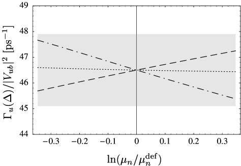
Figure 1: Residual scale dependence of $\Gamma_{u}(\Delta)$ for $\Delta=0.65$ GeV. The dashed line depicts the variation of $\mu_{h}$ about its default value $m_{b}/\sqrt{2}$, the dash-dotted line the variation of $\mu_{i}$ about $1.5$ GeV, and the dotted line the variation of $\bar{\mu}$ also about $1.5$ GeV. The highlighted area shows the combined perturbative uncertainty.

The purpose of this section is to investigate the individual contributions to $\Gamma_{u}(\Delta)$ that result from the corresponding terms in the weight function, as well as their residual dependence on the matching scales. For $\Delta=0.65$ GeV we find numerically

$$\frac{\Gamma_{u}(0.65\,{\rm GeV})}{|V_{ub}|^{2}\,{\rm ps}^{-1}} = 43.5\,\big{(}1+0.158\,\hbox{\scriptsize$[\alpha_{s}(\mu_{i})]$}-0.095\,\hbox{\scriptsize$[\alpha_{s}(\mu_{h})]$}+0.076\,\hbox{\scriptsize$[\alpha_{s}^{2}(\mu_{i})]$}$$ (38)

$$\hskip 34.14322pt\mbox{}-0.037\,\hbox{\scriptsize$[\alpha_{s}(\mu_{i})\alpha_{s}(\mu_{h})]$}+0.009\,\hbox{\scriptsize[kin]}-0.043\,\hbox{\scriptsize[hadr]}\big{)}=46.5\,.$$

The terms in parenthesis correspond to the contributions to the weight function arising at different orders in perturbation theory and in the $1/m_{b}$ expansion, as indicated by the subscripts. Note that the perturbative contributions from the intermediate scale are typically twice as large as the ones from the hard scale, which is also the naive expectation. Indeed, the two-loop $\alpha_{s}^{2}(\mu_{i})$ correction is numerically of comparable size to the one-loop $\alpha_{s}(\mu_{h})$ contribution. This confirms the importance of separating the scales $\mu_{i}$ and $\mu_{h}$. The contributions from kinematical and hadronic power corrections turn out to be numerically small, comparable to the two-loop corrections.

The weight function (3) is formally independent of the matching scales $\mu_{h}$, $\mu_{i}$, and $\bar{\mu}$. In Figure 1 we plot the residual scale dependence resulting from the truncation of the perturbative series. Each of the three scales is varied independently by a factor between $1/\sqrt{2}$ and $\sqrt{2}$ about its default value. The scale variation of $\mu_{i}$ is still as significant as the variation of $\mu_{h}$, even though the former is known at NNLO and the latter only at NLO. We have checked analytically that the result (3) is independent of $\mu_{i}$ through two-loop order, i.e. the residual scale dependence is an $O(\alpha_{s}^{3}(\mu_{i}))$ effect. In order to obtain a conservative estimate of the perturbative uncertainty in our predictions we add the individual scale dependencies in quadrature. This gives the gray band shown in the figure.

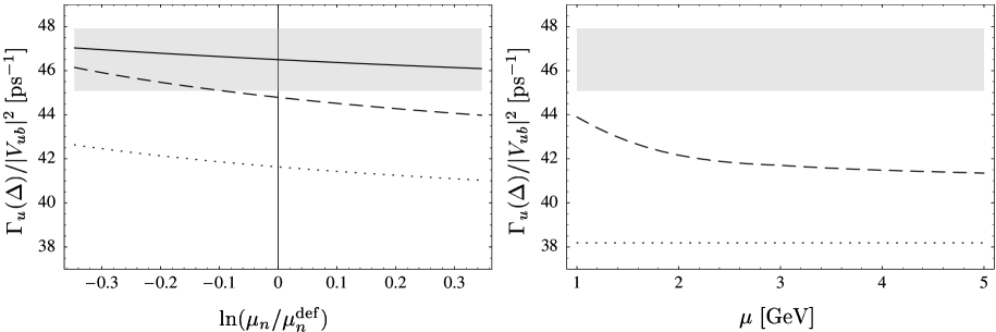
Figure 2: Convergence of the perturbative series and residual scale dependence. Left: RG-improved results at LO (dotted), NLO (dashed), and NNLO (solid) as a function of the scales $\mu_{i}$, $\mu_{h}$, $\bar{\mu}$, which are varied simultaneously about their default values. Right: Fixed-order results at tree-level (dotted) and one-loop order (dashed).

Figure 2 displays the result for $\Gamma_{u}(0.65\,\mbox{GeV})$ at different orders in RG-improved perturbation theory. At LO, we dismiss all $\alpha_{s}$ terms including the kinematical power corrections; however, leading logarithms are still resummed and give rise to a non-trivial dependence of $T_{0}$ on the coefficient $a$. At NLO, we include the $O(\alpha_{s}(\mu_{h}))$, $O(\alpha_{s}(\mu_{i}))$, and $O(\alpha_{s}(\bar{\mu}))$ contributions, but drop terms of order $\alpha_{s}^{2}(\mu_{i})$ or $\alpha_{s}(\mu_{i})\,\alpha_{s}(\mu_{h})$. At NNLO, we include all terms shown in (3). In studying the different perturbative approximations we vary the matching scales simultaneously (and in a correlated way) about their default values. Compared with Figure 1 this leads to a reduced scale variation. The gray bands in Figure 2 show the total perturbative uncertainty as determined above. While the two-loop NNLO contributions are sizable, we observe a good convergence of the perturbative expansion and a reduction of the scale sensitivity in higher orders. The right-hand plot in the figure contrasts these findings with the corresponding results in fixed-order perturbation theory, which are obtained from (3) by setting $\mu_{h}=\mu_{i}=\bar{\mu}=\mu$ and truncating the series at $O(\alpha_{s}(\mu))$ for consistency. We see that the fixed-order results are also rather insensitive to the value of $\mu$ unless this scale is chosen to be small; yet, the predicted values for $\Gamma_{u}$ are significantly below those obtained in RG-improved perturbation theory. We conclude that the small scale dependence observed in the fixed-order calculation does not provide a reliable estimator of the true perturbative uncertainty. In our opinion, a fixed-order calculation at a high scale is not only inappropriate in terms of the underlying dynamics of inclusive decay processes in the shape-function region, it is also misleading as a basis for estimating higher-order terms in the perturbative expansion.

4.2 Comments on the normalization of the photon spectrum

We mentioned in the Introduction that the use of the normalized photon spectrum is advantageous because event fractions in $\bar{B}\to X_{s}\gamma$ decay can be calculated more reliably than partial decay rates. In this section we point out another important advantage, namely that the perturbative series for the weight function $W(\Delta,P_{+})$ is much better behaved than that for $\widetilde{W}(\Delta,P_{+})$. The difference of the two weight functions lies in their normalizations, which are

$$W(\Delta,P_{+})\propto m_{b}^{3}\,T_{0}(a,\mu_{h})H_{\Gamma}(\mu_{h})\,,\qquad\widetilde{W}(\Delta,P_{+})\propto\frac{T_{0}(a,\mu_{h})}{[C_{7\gamma}^{\rm eff}(\mu_{h})]^{2}\,\overline{m}_{b}^{2}(\mu_{h})\,|H_{s}(\mu_{h})|^{2}}\,.$$ (39)

Here $H_{s}$ is the hard function in the factorized expression for the structure function ${\mathcal{F}}_{\gamma}$ in (4), which has been derived in [13]. Note that the two weight functions have a different dependence on the $b$-quark mass. In the case of $W$, three powers of $m_{b}$ enter through phase-space integrations in the total decay rate $\Gamma_{s}(E_{*})$, and it is therefore appropriate to use a low-scale subtracted quark-mass definition, such as the shape-function mass. In the case of $\widetilde{W}$, on the other hand, two powers of the running quark mass $\overline{m}_{b}(\mu_{h})$ enter through the definition of the dipole operator $O_{7\gamma}$, and it is appropriate to use a short-distance mass definition such as that provided by the $\overline{\rm MS}$ scheme. In practice, we write $\overline{m}_{b}(\mu_{h})$ as $\overline{m}_{b}(m_{b})$ times a perturbative series in $\alpha_{s}(\mu_{h})$.

The most pronounced effect of the difference in normalization is that the weight function $\widetilde{W}$ receives very large radiative corrections at order $\alpha_{s}(\mu_{h})$, which range between $-68\%$ and $-43\%$ when the scale $\mu_{h}$ is varied between $m_{b}$ and $m_{b}/2$. This contrasts the well-behaved perturbative expansion of the weight function $W$, for which the corresponding corrections vary between $-11\%$ and $-7\%$. In other words, the hard matching corrections for $\widetilde{W}$ are about six times larger than those for $W$. Indeed, these corrections are so large that in our opinion relation (2) should not be used for phenomenological purposes.

The different perturbative behavior of the hard matching corrections to the weight functions is mostly due to the mixing of the dipole operator $O_{7\gamma}$ with other operators in the effective weak Hamiltonian for $\bar{B}\to X_{s}\gamma$ decay. In order to illustrate this fact, consider the one-loop hard matching coefficients defined as

$$W\propto 1+k\,\frac{\alpha_{s}(\mu_{h})}{\pi}+\dots\,,\qquad\widetilde{W}\propto 1+\widetilde{k}\,\frac{\alpha_{s}(\mu_{h})}{\pi}+\dots\,.$$ (40)

With our default scale choices we have $k=-2.32+1.13=-1.19$, where the second contribution ($+1.13$) comes from operator mixing, which gives rise to the terms in the last two lines in (36). For the weight function $W$, this contribution has the opposite sign than the other terms, so that the combined value of $k$ is rather small. For the weight function $\widetilde{W}$, on the other hand, we find $\widetilde{k}=-1.58-5.52=-7.10$. Here the contribution from operator mixing is dominant and has the same sign as the remaining terms, thus yielding a very large value of $\widetilde{k}$. Such a large $O(\alpha_{s})$ correction was not observed in [11], because these authors chose to omit the contribution from operators mixing. Note that at a higher scale $\mu_{h}=m_{b}$, as was adopted in this reference, the situation is even worse. In that case we find $k=-2.81+1.19=-1.62$ and $\widetilde{k}=-0.66-9.13=-9.79$.

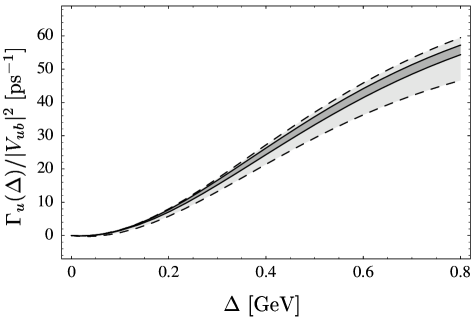
Figure 3: Perturbative uncertainties on $\Gamma_{u}(\Delta)$ encountered when using the weight function $W(\Delta,P_{+})$ (dark gray) or $\widetilde{W}(\Delta,P_{+})$ (light gray). In the latter case, the normalization of the photon spectrum is chosen such that the two predictions agree at $\Delta=0.65$ GeV for central values of the matching scales.

A visualization of the perturbative uncertainty is depicted in Figure 3, where predictions for $\Gamma_{u}(\Delta)$ are shown using either (1) or (2). In each case, the error band is obtained by varying the different scales about their default values, $\mu_{n}\in[\mu_{n}^{\rm def}/\sqrt{2},\mu_{n}^{\rm def}\sqrt{2}]$, and adding the resulting uncertainties in quadrature. The dark-gray band bordered by solid lines denotes the perturbative uncertainty of predictions when using the normalized photon spectrum, as in (1). (At the point $\Delta=0.65$ GeV this uncertainty is identical to the gray band depicted in Figures 1 and 2). The light-gray band bordered by dashed lines corresponds to the use of the absolute photon spectrum, as in (2). The difference in precision between the two methods would be even more pronounced if we used the higher default value $\mu_{h}=m_{b}$ for the hard matching scale. Obviously, the use of the normalized photon spectrum will result in a more precise determination of $|V_{ub}|$.

4.3 Comments on $\beta_{0}\alpha_{s}^{2}$ terms and scale separation

The separation of different momentum scales using RG techniques, which is one of the key ingredients of our approach, is well motivated by the dynamics of charmless inclusive $B$ decays in the shape-function region. Factorized expressions for the $B$-decay spectra involve hard functions renormalized at $\mu_{h}$ multiplied by jet and shape functions defined at a lower scale. While physics at or below the intermediate scale is very similar for $\bar{B}\to X_{u}\,l^{-}\bar{\nu}$ and $\bar{B}\to X_{s}\gamma$ (as is manifested by the fact that the leading shape and jet functions are universal), the physics at the hard scale in $\bar{B}\to X_{s}\gamma$ decay is considerably more complicated than in semileptonic decay, and it might even contain effects of New Physics. Therefore it is natural to respect the hierarchy $\mu_{h}\gg\mu_{i}$ and disentangle the various contributions, as done in the present work. In fact, our ability to calculate the dominant two-loop corrections is a direct result of this scale separation. Nevertheless, at a technical level we can reproduce the results of a fixed-order calculation by simply setting all matching scales equal to a common scale, $\mu_{h}=\mu_{i}=\bar{\mu}=\mu$. In this limit, the expressions derived in this work smoothly reduce to those obtained in conventional perturbation theory. While factorized expressions for the decay rates are superior to fixed-order results whenever there are widely separated scales in the problem, they remain valid in the limit where the different scales become of the same order.

In a recent publication, the $O(\beta_{0}\alpha_{s}^{2})$ BLM corrections [35] to the weight function $\widetilde{W}(\Delta,P_{+})$ in (2) were calculated in fixed-order perturbation theory [11]. For simplicity, only the contribution of the operator $O_{7\gamma}$ to the $\bar{B}\to X_{s}\gamma$ decay rate was included in this work. We note that without the contributions from other operators the expression for $\widetilde{W}$ is not renormalization-scale and -scheme invariant. Neglecting operator mixing in the calculation of $\widetilde{W}$ is therefore not a theoretically consistent approximation. However, having calculated the exact NNLO corrections at the intermediate scale allows us to examine some of the terms proportional to $\beta_{0}\alpha_{s}^{2}(\mu_{i})$ and compare them to the findings of [11]. In this way we confirm their results for the coefficients multiplying the logarithms $\ln^{n}[m_{b}(\Delta-P_{+})/\mu_{i}^{2}]$ with $n=1,2$ in (3). While the $\beta_{0}\alpha_{s}^{2}$ terms approximate the full two-loop coefficients of these logarithms arguably well, we stress that the two-loop constant at the intermediate scale is not dominated by terms proportional to $\beta_{0}$. Numerically we find

$$c^{(2)}_{0}=-47.4+39.6\,\frac{\beta_{0}}{25/3}+a\left[-31.8+38.8\,\frac{\beta_{0}}{25/3}\right]+O(a^{2})\,,$$ (41)

which means that the approximation of keeping only the BLM terms would overestimate this coefficient by almost an order of magnitude and give the wrong sign. This shows the importance of a complete two-loop calculation, as performed in the present work.

We believe that the perturbative approximations adopted in our paper, i.e. working to NNLO at the intermediate scale and to NLO at the hard scale, are sufficient for practical purposes in the sense that the residual perturbative uncertainty is smaller than other uncertainties encountered in the application of relation (1). Still, one may ask what calculations would be required to determine the missing $\alpha_{s}^{2}(\mu_{h})$ terms in the normalization of the weight function in (3), or at least the terms of order $\beta_{0}\alpha_{s}^{2}(\mu_{h})$. For the case of $\bar{B}\to X_{s}\gamma$ decay, the contribution of the operator $O_{7\gamma}$ to the normalized photon spectrum was recently calculated at two-loop order [36], while the contributions from other operators are known to $O(\beta_{0}\alpha_{s}^{2})$ [37]. What is still needed are the two-loop corrections to the double differential (in $P_{+}$ and $y$) $\bar{B}\to X_{u}\,l^{-}\bar{\nu}$ decay rate in (1).

4.4 Subleading corrections from hadronic structures

Due to the fact that different linear combinations of the subleading shape functions $\hat{t}(\hat{\omega})$, $\hat{u}(\hat{\omega})$, and $\hat{v}(\hat{\omega})$ enter the theoretical description of radiative and semileptonic decays starting at order $\Lambda_{\rm QCD}/m_{b}$, the weight function cannot be free of such hadronic structure functions. Consequently, we found in (3) all of the above subleading shape functions, divided by the leading shape function $\hat{S}(\hat{\omega})$. Our default model (32) for the subleading shape functions was chosen such that the combined effect of all hadronic power corrections could be absorbed into a single hadronic parameter $\Lambda_{\rm SSF}^{2}$. More generally, we define a function $\delta_{\rm hadr}(\Delta)$ via (a factor 2 is inserted for later convenience)

$$\Gamma_{u}(\Delta)=[\Gamma_{u}(\Delta)]_{\rm def}\left[1+2\delta_{\rm hadr}(\Delta)\right],$$ (42)

where $[\Gamma_{u}(\Delta)]_{\rm def}$ denotes the result obtained with the default model for the subleading shape functions. From (3), one finds that

$$\delta_{\rm hadr}(\Delta)=\frac{\int_{0}^{\Delta}\!dP_{+}\,(M_{B}-P_{+})^{4}\left[2(4-3a)\,h_{t}(P_{+})+(4-a)\,h_{u}(P_{+})+(8-13a+4a^{2})\,h_{v}(P_{+})\right]}{4(1-a)(3-a)\int_{0}^{\Delta}\!dP_{+}\,(M_{B}-P_{+})^{5}\,\hat{S}(P_{+})}\,,$$ (43)

where we have used that, at leading order in $\alpha_{s}$ and $\Lambda_{\rm QCD}/m_{b}$, the $\bar{B}\to X_{s}\gamma$ photon spectrum is proportional to $(M_{B}-P_{+})^{3}\,\hat{S}(P_{+})$. In the relation above, $h_{t}(\hat{\omega})\equiv\hat{t}(\hat{\omega})-[\hat{t}(\hat{\omega})]_{\rm def}$ etc. denote the differences between the true subleading shape functions and the functions adopted in our default model. By construction, these are functions with vanishing normalization and first moment.

The above expression for $\delta_{\rm hadr}(\Delta)$ is exact to the order we are working; however, in practice we do not know the precise form of the functions $h_{i}(\hat{\omega})$. Our goal is then to find a conservative bound, $|\delta_{\rm hadr}(\Delta)|<\epsilon_{\rm hadr}(\Delta)$, and to interpret the function $\epsilon_{\rm hadr}(\Delta)$ as the relative hadronic uncertainty on the value of $|V_{ub}|$ extracted using relation (1). To obtain the bound we scan over a large set of realistic models for the subleading shape functions. In [7], four different functions $h_{i}(\hat{\omega})$ were suggested, which can be added or subtracted (in different combinations) to each of the subleading shape functions. Together, this provides a large set of different models for these functions. To be conservative, we pick from this set the model which leads to the largest value of $|\delta_{\rm hadr}(\Delta)|$. The integrand in the numerator in (43) is maximized if all three $h_{i}(\hat{\omega})$ functions are equal to a single function, whose choice depends on the value of $\Delta$. In the denominator, we find it convenient to eliminate the shape function $\hat{S}(P_{+})$ in favor of the normalized photon spectrum. Working consistently to leading order, we then obtain

$$\epsilon_{\rm hadr}(\Delta)=\frac{5-5a+a^{2}}{(1-a)(3-a)}\,\frac{U(\mu_{h},\mu_{i})}{m_{b}^{3}}\,\max_{i}\frac{\displaystyle\left|\int_{0}^{\Delta}\!dP_{+}\,(M_{B}-P_{+})^{4}\,h_{i}(P_{+})\right|}{\displaystyle\int_{0}^{\Delta}\!dP_{+}\,(M_{B}-P_{+})^{2}\,\frac{1}{\Gamma_{s}(E_{*})}\,\frac{d\Gamma_{s}}{dP_{+}}}\,,$$ (44)

where as before $a=a_{\Gamma}(\mu_{h},\mu_{i})\approx 0.12$ for the default choice of matching scales, and $U(\mu_{h},\mu_{i})\approx 1.11$ [7].

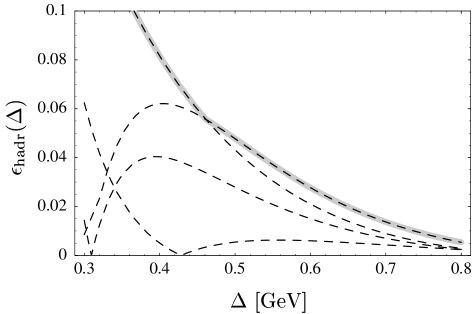
Figure 4: Estimates for the hadronic uncertainty $\epsilon_{\rm hadr}(\Delta)$ obtained from a scan over models for the subleading shape functions. The dashed lines correspond to the individual results for the four $h_{i}(\hat{\omega})$ functions suggested in [7]. The thick solid line, which covers one of the dashed lines, shows the maximum effect.

The result for the function $\epsilon_{\rm hadr}(\Delta)$ obtained this way is shown in Figure 4. We set the matching scales to their default values and use the model (37) for the photon spectrum, which is a good enough approximation for our purposes. From this estimate it is apparent that the effects of subleading shape functions are negligible for large values $\Delta\gg\Lambda_{\rm QCD}$ and moderate for $\Delta\sim\Lambda_{\rm QCD}$, which is the region of interest for the determination of $|V_{ub}|$. In the region $\Delta<0.3$ GeV the accuracy of the calculation deteriorates. For example, we find $\epsilon_{\rm hadr}=2.0\%$ for $\Delta=0.65$ GeV, $\epsilon_{\rm hadr}=4.8\%$ for $\Delta=0.5$ GeV, and $\epsilon_{\rm hadr}=8.2\%$ for $\Delta=0.4$ GeV.

5 Conclusions

Model-independent relations between weighted integrals of $\bar{B}\to X_{s}\gamma$ and $\bar{B}\to X_{u}\,l^{-}\bar{\nu}$ decay distributions, in which all reference to the leading non-perturbative shape function is avoided, offer one of the most promising avenues to a high-precision determination of the CKM matrix element $|V_{ub}|$. In order to achieve a theoretical precision of better than 10%, it is necessary to include higher-order corrections in $\alpha_{s}$ and $\Lambda_{\rm QCD}/m_{b}$ in this approach.

In the present work, we have calculated the weight function $W(\Delta,P_{+})$ in the relation between the hadronic $P_{+}=E_{X}-|\vec{P}_{X}|$ spectra in the two processes, integrated over the interval $0\leq P_{+}\leq\Delta$. Based on QCD factorization theorems for the differential decay rates, we have derived an exact formula (15) that allows for the calculation of the leading-power weight function to any order in perturbation theory. We have calculated the $\Delta$- and $P_{+}$-dependent terms in the weight function exactly at next-to-next-to-leading order (NNLO) in renormalization-group improved perturbation theory, including two-loop matching corrections at the intermediate scale $\mu_{i}\sim\sqrt{m_{b}\Lambda_{\rm QCD}}$ and three-loop running between the intermediate scale and the hard scale $\mu_{h}\sim m_{b}$. The only piece missing for a complete prediction at NNLO is the two-loop hard matching correction to the overall normalization of the weight function. A calculation of the $\alpha_{s}^{2}(\mu_{h})$ term would require the knowledge of both decay spectra at two-loop order, which is currently still lacking. We also include various sources of power corrections. Power corrections from phase-space factors are treated exactly. The remaining hadronic and kinematical power corrections are given to first order in $\Lambda_{\rm QCD}/m_{b}$ and to the order in perturbation theory to which they are known.

A dedicated study of the perturbative behavior of our result for the weight function has been performed for the partial $\bar{B}\to X_{u}\,l^{-}\bar{\nu}$ decay rate $\Gamma_{u}(\Delta)$ as obtained from the right-hand side of relation (1). It exhibits good convergence of the expansion and reduced scale sensitivity in higher orders. We find that corrections of order $\alpha_{s}^{2}(\mu_{i})$ at the intermediate scale are typically as important as first-order $\alpha_{s}(\mu_{h})$ corrections at the hard scale. We have also seen that fixed-order perturbation theory significantly underestimates the value of $\Gamma_{u}(\Delta)$, even though the apparent stability with respect to scale variations would suggest a good perturbative convergence. In order to obtain a well-behaved expansion in powers of $\alpha_{s}(\mu_{h})$, it is important to use the normalized photon spectrum in relation (1). A similar relation involving the differential $\bar{B}\to X_{s}\gamma$ decay rate receives uncontrollably large matching corrections at the hard scale and is thus not suitable for phenomenological applications. At next-to-leading order in the $1/m_{b}$ expansion, the weight function receives terms involving non-perturbative subleading shape functions, which cannot be eliminated. Our current ignorance about the functional forms of these functions leads to a hadronic uncertainty, which we have estimated by scanning over a large set of models. We believe that a reasonable estimate of the corresponding relative uncertainty $\epsilon_{\rm hadr}$ on $|V_{ub}|$ is given by the solid line in Figure 4.

Let us summarize our main result for the partial $\bar{B}\to X_{u}\,l^{-}\bar{\nu}$ decay rate with a cut $P_{+}\leq 0.65$ GeV, which is close to the charm threshold $M_{D}^{2}/M_{B}$, and present a detailed list of the various sources of theoretical uncertainties. We find

$$\Gamma_{u}(0.65\,{\rm GeV}) = \left(46.5\pm 1.4\,\hbox{\scriptsize[pert]}\,\pm 1.8\,\hbox{\scriptsize[hadr]}\,\pm 1.8\,\hbox{\scriptsize[$m_{b}$]}\,\pm 0.8\,\hbox{\scriptsize[pars]}\,\pm 2.8\,\hbox{\scriptsize[norm]}\,\right)|V_{ub}|^{2}\,{\rm ps}^{-1}$$ (45)

$$= (46.5\pm 4.1)\,|V_{ub}|^{2}\,{\rm ps}^{-1}\,,$$

where the central value is derived assuming that the $\bar{B}\to X_{s}\gamma$ photon spectrum can be accurately described by the function (37). The errors refer to the perturbative uncertainty as estimated in Section 4.1, the uncertainty due to the ignorance about subleading shape functions as discussed in Section 4.4, the error in the value of the $b$-quark mass, other parametric uncertainties from variations of $m_{c}$, $m_{s}$, and $\lambda_{1}$, and finally a 6% uncertainty in the calculation of the normalization of the photon spectrum [13]. To a good approximation the errors scale with the central value. The above numbers translate into a combined theoretical uncertainty of 4.4% on $|V_{ub}|$ when added in quadrature.

Acknowledgments: We thank the Institute of Nuclear Theory at the University of Washington, where part of this research has been performed. The work of M.N. was supported in part by a Research Award of the Alexander von Humboldt Foundation. The work of B.O.L. was supported in part by funds provided by the U.S. Department of Energy under cooperative research agreement DE-FC02-94ER40818. The research of M.N. and G.P. was supported by the National Science Foundation under Grant PHY-0355005.

References

- [1] M. Neubert, Phys. Rev. D 49, 3392 (1994) [hep-ph/9311325].
- [2] M. Neubert, Phys. Rev. D 49, 4623 (1994) [hep-ph/9312311].
- [3] I. I. Y. Bigi, M. A. Shifman, N. G. Uraltsev and A. I. Vainshtein, Int. J. Mod. Phys. A 9, 2467 (1994) [hep-ph/9312359].
- [4] T. Mannel and S. Recksiegel, Phys. Rev. D 60, 114040 (1999) [hep-ph/9904475].
- [5] U. Aglietti, M. Ciuchini and P. Gambino, Nucl. Phys. B 637, 427 (2002) [hep-ph/0204140].
- [6] S. W. Bosch, B. O. Lange, M. Neubert and G. Paz, Phys. Rev. Lett. 93, 221801 (2004) [hep-ph/0403223].
- [7] B. O. Lange, M. Neubert and G. Paz, hep-ph/0504071, Phys. Rev. D (in press).
- [8] A. K. Leibovich, I. Low and I. Z. Rothstein, Phys. Rev. D 61, 053006 (2000) [hep-ph/9909404].
- [9] A. K. Leibovich, I. Low and I. Z. Rothstein, Phys. Lett. B 486, 86 (2000) [hep-ph/0005124].
- [10] M. Neubert, Phys. Lett. B 513, 88 (2001) [hep-ph/0104280].
- [11] A. H. Hoang, Z. Ligeti and M. Luke, Phys. Rev. D 71, 093007 (2005) [hep-ph/0502134].
- [12] A. L. Kagan and M. Neubert, Eur. Phys. J. C 7, 5 (1999) [hep-ph/9805303].
- [13] M. Neubert, Eur. Phys. J. C 40, 165 (2005) [hep-ph/0408179].
- [14] C. W. Bauer and A. V. Manohar, Phys. Rev. D 70, 034024 (2004) [hep-ph/0312109].
- [15] S. W. Bosch, B. O. Lange, M. Neubert and G. Paz, Nucl. Phys. B 699, 335 (2004) [hep-ph/0402094].
- [16] M. Neubert, hep-ph/0506245, Phys. Rev. D (in press).
- [17] M. Neubert, Phys. Lett. B 612, 13 (2005) [hep-ph/0412241].
- [18] G. P. Korchemsky and A. V. Radyushkin, Nucl. Phys. B 283, 342 (1987).
- [19] I. A. Korchemskaya and G. P. Korchemsky, Phys. Lett. B 287, 169 (1992).
- [20] S. Moch, J. A. M. Vermaseren and A. Vogt, Nucl. Phys. B 688, 101 (2004) [hep-ph/0403192].
- [21] F. De Fazio and M. Neubert, JHEP 9906, 017 (1999) [hep-ph/9905351].
- [22] C. W. Bauer, D. Pirjol and I. W. Stewart, Phys. Rev. D 65, 054022 (2002) [hep-ph/0109045].
- [23] C. W. Bauer, M. E. Luke and T. Mannel, Phys. Rev. D 68, 094001 (2003) [hep-ph/0102089].
- [24] A. K. Leibovich, Z. Ligeti and M. B. Wise, Phys. Lett. B 539, 242 (2002) [hep-ph/0205148].
- [25] C. W. Bauer, M. Luke and T. Mannel, Phys. Lett. B 543, 261 (2002) [hep-ph/0205150].
- [26] M. Neubert, Phys. Lett. B 543, 269 (2002) [hep-ph/0207002].
- [27] C. N. Burrell, M. E. Luke and A. R. Williamson, Phys. Rev. D 69, 074015 (2004) [hep-ph/0312366].
- [28] K. S. M. Lee and I. W. Stewart, Nucl. Phys. B 721, 325 (2005) [hep-ph/0409045].
- [29] S. W. Bosch, M. Neubert and G. Paz, JHEP 0411, 073 (2004) [hep-ph/0409115].
- [30] M. Beneke, F. Campanario, T. Mannel and B. D. Pecjak, JHEP 0506, 071 (2005) [hep-ph/0411395].
- [31] J. Chay, C. Kim and A. K. Leibovich, Phys. Rev. D 72, 014010 (2005) [hep-ph/0505030].
- [32] A. F. Falk and M. Neubert, Phys. Rev. D 47, 2965 (1993) [hep-ph/9209268].
- [33] E. Gamiz, M. Jamin, A. Pich, J. Prades and F. Schwab, Phys. Rev. Lett. 94, 011803 (2005) [hep-ph/0408044].
- [34] C. Aubin et al. [HPQCD Collaboration], Phys. Rev. D 70, 031504 (2004) [hep-lat/0405022].
- [35] S. J. Brodsky, G. P. Lepage and P. B. Mackenzie, Phys. Rev. D 28, 228 (1983).
- [36] K. Melnikov and A. Mitov, Phys. Lett. B 620, 69 (2005) [hep-ph/0505097].
- [37] Z. Ligeti, M. E. Luke, A. V. Manohar and M. B. Wise, Phys. Rev. D 60, 034019 (1999) [hep-ph/9903305].