Non-standard Hamiltonian effects on neutrino oscillations
Mattias Blennow111Email: emb@kth.se, Tommy Ohlsson222Email: tommy@theophys.kth.se, and Walter Winter333Email: winter@ias.edu
,22footnotemark: 2Department of Theoretical Physics, School of Engineering Sciences,
Royal Institute of Technology (KTH) – AlbaNova University Center,
Roslagstullsbacken 21, 106 91 Stockholm, Sweden
33footnotemark: 3School of Natural Sciences, Institute for Advanced Study,
Einstein Drive, Princeton, NJ 08540, USA
Abstract
We investigate non-standard Hamiltonian effects on neutrino oscillations, which are effective additional contributions to the vacuum or matter Hamiltonian. Since these effects can enter in either flavor or mass basis, we develop an understanding of the difference between these bases representing the underlying theoretical model. In particular, the simplest of these effects are classified as “pure” flavor or mass effects, where the appearance of such a “pure” effect can be quite plausible as a leading non-standard contribution from theoretical models. Compared to earlier studies investigating particular effects, we aim for a top-down classification of a possible “new physics” signature at future long-baseline neutrino oscillation precision experiments. We develop a general framework for such effects with two neutrino flavors and discuss the extension to three neutrino flavors, as well as we demonstrate the challenges for a neutrino factory to distinguish the theoretical origin of these effects with a numerical example. We find how the precision measurement of neutrino oscillation parameters can be altered by non-standard effects alone (not including non-standard interactions in the creation and detection processes) and that the non-standard effects on Hamiltonian level can be distinguished from other non-standard effects (such as neutrino decoherence and decay) if we consider specific imprint of the effects on the energy spectra of several different oscillation channels at a neutrino factory.
1 Introduction
Neutrino physics has entered the era of precision measurements of the fundamental neutrino parameters such as neutrino mass squared differences and leptonic mixing parameters, and neutrino oscillations are the most credible candidate for describing neutrino flavor transitions. Nevertheless, there might be other sub-leading mechanisms participating in the total description of neutrino flavor transitions. Thus, in this paper, we will investigate such mechanisms on a fundamental level, which will give rise to non-standard effects on the ordinary framework of neutrino oscillations.
In a previous paper [1], we have studied non-standard effects on probability level based on “damping signatures”, which were phenomenologically introduced in the neutrino oscillation probabilities. However, in this paper, we will investigate so-called non-standard Hamiltonian effects, which are effects on Hamiltonian level rather than on probability level. Recently, three different main categories of non-standard Hamiltonian effects have been discussed in the literature. These categories are non-standard interactions (NSI), flavor changing neutral currents (FCNC), and mass varying neutrinos (MVN or MaVaNs). In addition, other effects which result in effective additions to the Hamiltonian have been studied, such as from extra dimensions [2]. Below, we will shortly review the categories of effects which can be studied using this framework.
In general, in many models, neutrino masses come together with NSI, which means that the evolution of neutrinos passing through matter is modified by non-standard potentials due to coherent forward-scattering of NSI processes , where and is a fermion in matter.111Note that, in general, the production and detection vertices could also be modified. However, in this paper, we focus on the neutrino oscillation probabilities which, in the limit of ultrarelativistic neutrinos, decouple from the creation and detection processes. The effective NSI potentials are given by , where is the Fermi coupling constant, is the down quark number density, and ’s are small parameters describing the NSI [3]. See, e.g., Ref. [4] for a recent review. Furthermore, matter-enhanced neutrino oscillations in presence of -induced FCNC have been studied in the literature [5, 6, 7]. See also, e.g., Refs. [8, 9] for some earlier contributions. Especially, NSI and FCNC have been investigated in several references for many different scenarios such as for solar [10, 11, 12, 13], atmospheric [14, 15, 16, 17, 18], supernova [19], and other astrophysical neutrinos as well as for CP violation [20], the LSND experiment [21], beam experiments [22], and neutrino factories [23, 24, 25, 26, 27, 28].
The idea of MVN was proposed by Fardon et al. in Refs. [29, 30]. This idea is based on the dark energy of the Universe being neutrinos which can act as a negative pressure fluid and be the origin of cosmic acceleration. Furthermore, several continuation works on MVN have been performed in the context of scenarios for the Sun and the solar neutrino deficit [31, 32], but also in various other contexts [33, 34, 35, 36, 37, 38, 39, 40, 41, 42, 43, 44, 45]. In addition, it should be mentioned that neutrinos with variable masses have also been studied earlier than the idea of MVN [46, 47, 48, 49, 29].
While earlier studies have discussed individual theoretical models and their effects on future neutrino oscillation experiments (bottom-up), our approach will be the top-down. We start from general assumptions to investigate the properties of non-standard Hamiltonian effects, and later apply them to specific models and discuss how to identify individual effects. The goal of this approach is the classification of a possible “new physics” signature in future long-baseline neutrino oscillation experiments. Although it is very likely that such a signature will fit many different non-standard models, it has hardly been discussed in the literature how to distinguish (even qualitatively) different theoretical models which could all describe this effect, and what the methods for that identification could be. For this purpose, we make rather unspecific assumptions for the particular type of effect and rather assume that the theoretical model will predict a leading effect which can be considered to be of a “simple” form in a specific basis (“pure” effect), which can be either flavor (or mass) conserving or flavor (or mass) violating.
The paper is organized as follows: First, in Sec. 2, we define non-standard Hamiltonian effects as effective additional contributions to the vacuum Hamiltonian similar to matter effects. The definition is performed for neutrino flavors. Next, in Sec. 3, we specialize our discussion to two neutrino flavors, where we derive the effective neutrino parameters as well as the resonance conditions in both flavor and mass bases including non-standard Hamiltonian effects. We also discuss experimental strategies to test and identify non-standard Hamiltonian effects at the example of flavor transitions. Then, in Sec. 4, we study some aspects of the generalization to three-flavor case, whereas in Sec. 5, we give a numerical example of how non-standard Hamiltonian effects can affect a realistic experimental setup and discuss how to tell non-standard Hamiltonian effects apart from damping effects. Finally, we summarize our results and present our conclusions in Sec. 6.
2 Parameterization of non-standard Hamiltonian effects
In the standard neutrino oscillation framework with flavors, the Hamiltonian in vacuum is given by
| (1) |
in flavor basis, where is the neutrino energy, is the leptonic mixing matrix, and is the mass of the th neutrino mass eigenstate. Any Hermitian non-standard Hamiltonian effect will alter this vacuum Hamiltonian into an effective Hamiltonian
| (2) |
where is the effective addition to the vacuum Hamiltonian. We note that this reminds of neutrino mixing and oscillations in matter [8] with given by a diagonal matrix with the effective matter potentials on the diagonal, i.e.,
| (3) |
where is the ordinary matter potential, is the Fermi coupling constant, is the electron number density (resulting from coherent forward-scattering of neutrinos), is the nucleon number density, and is the unit matrix222If sterile neutrinos are present, then there is no interaction between the sterile neutrinos and the matter through which they propagate. Thus, the term is replaced by a projection operator on the active neutrino states.. Just as the presence of matter affects the effective neutrino mixing parameters, the effective neutrino mixing parameters will be affected by any non-standard Hamiltonian effect. In the remainder of this text, we will treat the effective Hamiltonian
| (4) |
i.e., we will treat the non-standard effects along with the matter effects. However, in Sec. 4, we treat only the part in order to obtain the parameters of the Hamiltonian to which the standard matter effects are then added. Since standard matter effects are generally taken into account, will be mistaken for the vacuum Hamiltonian if the non-standard effects are not considered.
Since any part of the effective Hamiltonian that is proportional to the unit matrix only contributes with an overall phase to the final neutrino state, it will not affect the neutrino oscillation probabilities. This means that we may assume to be traceless and also that we may subtract from the effective Hamiltonian to make it traceless. Any traceless Hermitian matrix may be written as
| (5) |
where the ’s are real numbers, the ’s are the generators of the Lie algebra (i.e., is an element of the Lie algebra), and is the number of generators. Hence, clearly, any non-standard Hamiltonian effect is parameterized by the numbers . In summary, we choose the coefficients of the generators of the Lie algebra to parameterize any non-standard Hamiltonian effect.
Furthermore, in any basis (e.g., flavor or mass basis), we may introduce generators such that generators are off-diagonal with only two real non-zero entries, generators are off-diagonal with only two imaginary non-zero entries, and generators are diagonal with real entries. For example, in the case of , we have the Pauli matrices
| (6) |
We will denote the set of generators which are of the form in flavor basis by and the set of generators which are of this form in mass basis by . Obviously, in flavor basis, we have the relations
| (7) |
where, in the case of two neutrino flavors,
is the two-flavor leptonic mixing matrix and is the corresponding mixing angle (when treating the three-flavor case, we will use the standard parameterization of the leptonic mixing with three mixing angles , , , and one CP violating phase ). This implies that and would be equal if there was no mixing in the leptonic sector. Furthermore, it is obvious that the matrices can be written as linear combinations of the matrices and vice versa. Therefore, there is, in principle, no difference between effects added in flavor or mass basis if one allows for the most general form of the non-standard contribution.
We now define any non-standard effect as a “pure” flavor or mass effect if the corresponding effective contribution to the Hamiltonian is given by
| (8) |
respectively, where . This means that we restrict the “pure” effects to be of very specific types, where the actual forms are very simple in a given basis.333Because of our choice to use the Pauli matrices, a “pure” effect corresponds to the interaction of two flavor or mass eigenstates. This is also the reason for choosing to work with the Pauli matrices. In addition, it is also interesting to keep the real and complex parts of the off-diagonal entries separate (i.e., not working with the complex matrix elements directly, but rather a set of real parameters) in order to investigate the possibilities of probing CP violation effects. Given the possible theoretical origin, this approach is quite plausible if one assumes that the underlying theoretical model will produce one leading flavor (or mass) changing or conserving effect. Generally, the parameter can depend on many different quantities, e.g., the matter density or the neutrino energy. In particular, the dependence on the neutrino energy (“spectral dependence”) may allow for the unambiguous identification, or, in the case of mass-varying neutrinos, the matter density dependence may indicate this type of effect. However, any approach investigating such dependencies has to use specific models, and the actual representation by Nature may easily be overseen. Therefore, we do not require this information in this study and rather investigate the generic impact of effects in the flavor or mass basis. In addition, we note that the matter density or energy dependence of the non-standard effects should be very weak for a given terrestrial experiment with a specific matter density profile. Only for effects motivated by MVN, i.e., mass effects, we will use the same energy dependence as for the masses themselves for numerical simulations. In general, if a large span of energies is available, one should of course also try to distinguish different specific models through their different energy dependencies.
This choice of pure effects implies that only one of the generators of the Lie algebra is present, since a general linear combination, such as Eq. (5), can always be interpreted in both bases. Thus, we define a flavor or mass conserving (violating) effect as any effect where the effective contribution to the Hamiltonian is diagonal (off-diagonal) in the corresponding basis.444Strictly speaking, our definition distinguishes (in two-flavors) off-diagonal additions proportional to (real) or (complex). We note that a pure flavor (mass) violating effect corresponds to some interaction between two flavor (mass) eigenstates. For example, the generators and correspond to flavor violating (or changing) effects, whereas corresponds to flavor conserving effects. In summary, if we detect an arbitrary non-standard effect, it is the simple form in flavor or mass basis which makes it a flavor or mass effect by our definition. This approach can be justified by the fact that the simplest models for non-standard effects from the underlying theory correspond to specific patterns for the effective addition to the Hamiltonian. Therefore, our definition of a “pure” effect is a conceptually new one and it refers to a class of effects, which can be interpreted in different ways. However, since simplicity is a basic concept in physics, this concept allows the choice of the most “natural” non-standard effects for further testing.
The case of non-standard Hamiltonian effects on three-flavor neutrino oscillations, i.e., the case of , is quite similar to the one described above for the two-flavor case. Instead of the Pauli matrices, which are a basis of the Lie algebra, we now have to use the eight Gell-Mann matrices, which span the Lie algebra. Out of the Gell-Mann matrices, three are off-diagonal with two real entries, three are off-diagonal with two imaginary entries, and two are diagonal with real entries. Even though the principle of the three-flavor case is the same as that of the two-flavor case, it introduces many more parameters (more leptonic mixing angles, the complex phase in the leptonic mixing matrix, the extra mass squared difference, and the extra degrees of freedom for the non-standard effects), and therefore, turns out to be much more cumbersome to handle than the two-flavor case. In the following, we will therefore start by treating the two-flavor case in some detail and then continue by studying the similarities and differences when approaching the full three-flavor case.
As far as the classification of current models in our notation is concerned, NSI and FCNC will be flavor effects, whereas MVN will produce mass effects. In general, NSI can be of two types: flavor changing (FC) and non-universal (NU) [4]. The off-diagonal elements of the effective NSI potential , where , correspond to FC, whereas the differences in the diagonal elements correspond to NU. In addition, FCNC are flavor violating effects and MVN can be mass conserving. In principle, for our purposes, there is no difference between FC NSI and FCNC.
3 Non-standard Hamiltonian effects in the two-flavor limit
In this section, we study the general implications of non-standard Hamiltonian effects in the two-flavor limit. We discuss the effective parameter mapping including non-standard effects, and then, we apply it to a two-flavor limit as an example.
3.1 Parameter mapping in two flavors
In Appendix A, we describe the general formalism of the two-flavor scenario, which can be used to obtain the results in this section. First, we discuss effects given in flavor basis, which are effects expanded in [cf., Eq. (7)]. In this case, flavor conserving effects will be contributions to the total Hamiltonian on the form , where , whereas flavor violating effects will be contributions on the form , where . In flavor basis, the new effective parameters are given by
| (9) | ||||
| (10) |
where
| (11) |
is the normalized length of the Hamiltonian vector (see Appendix A), is the effective mass squared difference in flavor basis, and is the effective mixing angle in flavor basis.555Note that may also change the effective Majorana phase. In addition, the resonance condition is found to be
| (12) |
which is clearly nothing but a somewhat modified version of the Mikheyev–Smirnov–Wolfenstein (MSW) resonance condition [8, 50, 51]. From the resonance condition in Eq. (12), it is easy to observe that the resonance is present for some energy if and only if
| (13) |
where is dependent on the mass hierarchy, is dependent on if we are studying neutrinos or anti-neutrinos, and is dependent on the ratio between and the matter potential [ being equal to if and only if has a magnitude larger than and is of opposite sign to ]. Note that if there are flavor violating contributions added to the Hamiltonian, then these do not change the resonance condition. The sign of can be made positive by reordering the mass eigenstates in the case of two neutrino flavors. However, we keep this term as it is, since this is not possible in the case of three neutrino flavors. This resonance condition can be easily understood, since the effective contribution to the Hamiltonian from any flavor violating effect will be parallel to the plane, i.e., these contributions are off-diagonal.
If we choose to describe the non-standard addition to the Hamiltonian in the mass eigenstate basis, then we find that the mixing parameters are given by
| (14) | ||||
| (15) |
where
| (16) |
and the resonance condition becomes
| (17) |
Note that both mass conserving effects and mass violating effects enter into the resonance condition, whereas only the flavor conserving effects entered in the corresponding expression in the flavor basis [cf., Eq. (12)]. This is due to the fact that the changes of the Hamiltonian vector from such effects are not parallel to the plane (in flavor basis, see Appendix A), i.e., both of these effects affect the diagonal terms of the total Hamiltonian. However, does not enter into the resonance condition, since , i.e., the change of the Hamiltonian is off-diagonal also in the flavor basis.
3.2 Interpretation of experiments in the two-flavor limit
Since a general analytic discussion of three-flavor neutrino oscillations including non-standard Hamiltonian effects would be very complicated, we focus on two neutrino flavors in this section. This approach can be justified if one assumes that the other contributions are exactly known or the two-flavor probabilities dominate. Of course, for short-term applications, small non-standard effects might be confused with other small effects such as effects [27]. Thus, a comprehensive quantitative discussion would be very complicated at present.
In three-flavor neutrino oscillations, we can construct several interesting two-flavor limits of the probabilities including non-standard effects related to two-flavor neutrino oscillations (see, e.g., Ref. [52]):
| (18) | |||||
| (19) | |||||
| (20) | |||||
| (21) |
Note that all of these probabilities also contain the standard matter effects except from . In general, the generators (the Gell-Mann matrices) will give the degrees of freedom for non-standard Hamiltonian effects with three flavors. However, when studying the effective two-flavor neutrino oscillations, we only use the Gell-Mann matrices which are the equivalents of the Pauli matrices in the two-flavor sector that is studied. In addition, one can create two-flavor limits for oscillations into sterile neutrinos, such as in Ref. [2]. In the following, we will focus on small mixing and the case of Eq. (20) for illustration. We discuss the large mixing case in Appendix B. In addition, see Appendix C for subtleties with the definitions of the effective two-flavor scenarios.
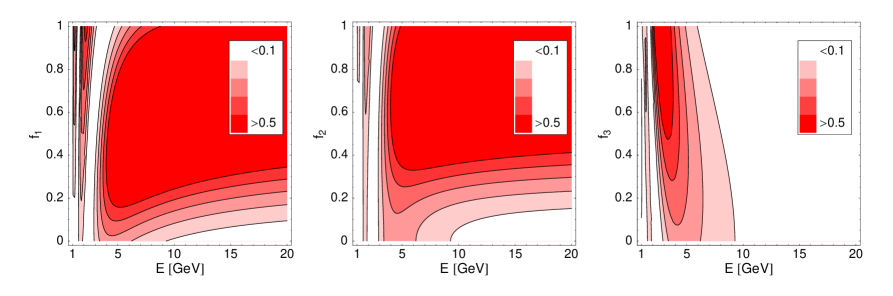
the neutrino oscillation appearance probability for two flavors with small mixing, where the effects of the ’s are parameterized relative to the matter effects (i.e., “1” on the vertical axis corresponds to an effect with and “0” to no non-standard effects). In this figure, many of the following analytic observations are visualized. The resonance condition in Eq. (12) can always be fulfilled for the matter resonance () by an appropriate choice of energy, baseline, neutrinos or antineutrinos, and oscillation channel. Obviously, we can read off from Eq. (10) that at the resonance , where the matter resonance condition can be influenced by according to Eq. (12). Therefore, the magnitude of at the resonance (but not necessarily ) is independent of , , and by definition. However, can shift the position of the resonance (such as in energy space). If we choose an energy far above the resonance energy and (), then we have
| (22) |
This means that and can, for large enough energies, enhance a flavor transition, i.e., they increase the oscillation amplitude. In principle, one could distinguish from by a measurement at two different energies, because the mixed term from the square in the numerator of Eq. (22) has a linear (instead of quadratic) energy dependence. In practice, such a discrimination should be very hard. In addition, the quantity can play the same role as the matter potential , i.e., it can change the flavor transition for large energies. It is also obvious from Eqs. (10) and (11) that can affect the matter resonance energy and that it is directly correlated with the matter potential , i.e., one cannot establish effects more precisely than the matter density uncertainty.
In Sec. 3.1, we have also discussed mass effects, such as coming from MVN. Since a pure or effect translates into a combination of and [cf., Eq. (46)], we expect to find a mixture of and effects, i.e., both and effects have to be present. Thus, if we assume that there is only one dominating “pure” non-standard contribution (, , , , , or ), then this simultaneous presence points toward a mass effect. Clearly, an effect, on the other hand, cannot be distinguished from an effect [cf., Eq. (46)]. A different property of , which is not so obvious from Sec. 3.1, but very obvious already from Eqs. (1), (2), and (7): Since is diagonal in mass basis, it corresponds to an energy dependent shift of the vacuum mass squared difference. As a consequence, in vacuum, the effective mixing angle is not modified by [cf., Eq. (15)]. Thus, the oscillation amplitudes are not modified by , but the oscillation pattern shifts (contrary to effects, where also the amplitude changes). In this case, the resonance condition becomes meaningless and the amplitude becomes . Note that a direct test using one experiment only makes it hard to identify mass effects uniquely if they are introduced with the same energy dependence as the vacuum masses (because they can be rotated away by a different set of neutrino oscillation parameters). Thus, other methods might be preferable, such as modified MSW transitions in the Sun [31, 32] or reactor experiments comparing air and matter oscillations [53]).
Another class of effects has been discussed by Blennow et al. in Ref. [1]. In this study, so-called “damping effects” could describe modifications on probability level instead of Hamiltonian level (such as neutrino decay, absorption, wave packet decoherence, oscillations into sterile neutrinos, quantum decoherence, averaging, etc.). It is obvious from Eq. (3) in Ref. [1] that these damping effects do not alter the oscillation frequency, while we can read off from Eqs. (9) and (11) that it is a general feature of non-standard Hamiltonian effects that the oscillation frequency is changed. However, for damping effects, the oscillation amplitude can be damped either by a damping of the overall probability (“decay-like damping”) or by the oscillating terms only (“decoherence-like damping”). In the first case, the total probability of finding a neutrino in any neutrino state is damped for all energies, whereas in the second case, it is constantly equal to one while the individual neutrino oscillation probabilities are damped in the oscillation maxima and enhanced in the oscillation minima. Since all (small) effects one could imagine in quantum field theory, involving the modification of fundamental interactions or propagations, can be described by either coherent or incoherent addition of amplitudes, one can expect that the two classes of Hamiltonian and probability (damping) effects can cover all possible effects. However, in practice, potential energy, environment, and explicit time dependencies (such as from a matter potential) can make life more complicated.
4 Three-flavor effects
As was stated in the Sec. 2, the general three-flavor case is quite complicated. However, if we assume that the non-standard effects are small, then we can use perturbation theory to derive expressions for the change in the neutrino oscillation parameters. For example, the elements of the effective mixing matrix are given by
| (23) |
where is the eigenstate of the full Hamiltonian. To first order in perturbation theory, we have
| (24) |
and thus, we find
| (25) |
or, in terms of the non-standard addition given in flavor basis,
| (26) |
We note that this approach is valid only if . If this is not valid, then we have to use degenerate perturbation theory in order to obtain valid results.
It was discussed in Refs. [26, 27], that if is small enough, then possible NSI in the creation, propagation, and detection processes may mimic the effects of a larger (this can also be the case for other effects which are not usually treated along with neutrino oscillations, such as damping effects [1]). Here, we consider only the propagation effects separately and consider how this alone could affect the determination of . The reason for doing so is that, while NSI can also affect the creation and detection processes, other non-standard effects, e.g., MVN, may not. With the perturbation theory approach described above, this becomes very transparent, and is probably one of the most interesting applications of non-standard effects. In any experimental setup, the value of the mixing angle is determined by the modulus of the element of the neutrino mixing matrix . If we include non-standard effects, then the effective counterpart of this element is given by
| (27) | |||||
where we have made a series expansion to first order in and disregarded terms of second order in both and .
If is smaller than or of equal size to the other terms in this expression, then the determined by an experiment will not be the actual unless the non-standard effects are taken into account. It is worth to notice that if , then and only the imaginary part of will enter into the expression for , indicating that if the leading term is the one containing , then the effective CP violating phase will be . Another interesting observation is that even if there are no non-standard effects, there is a term proportional to in this expression. Because of the different matter potentials for and due to loop-level effects, this quantity will be of the order .
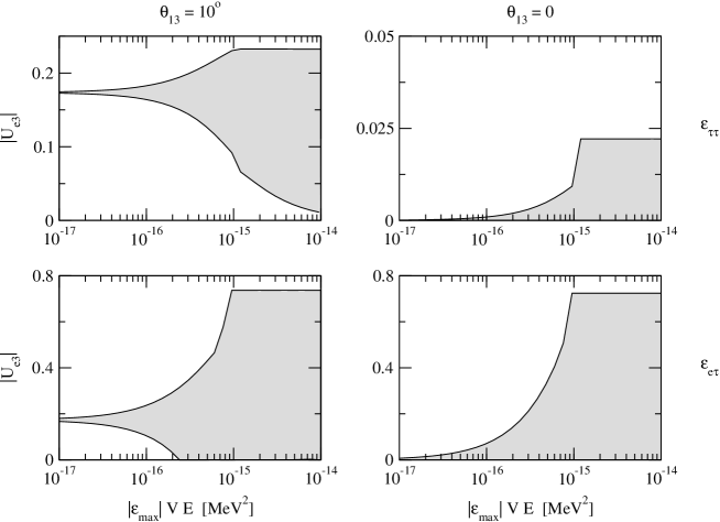
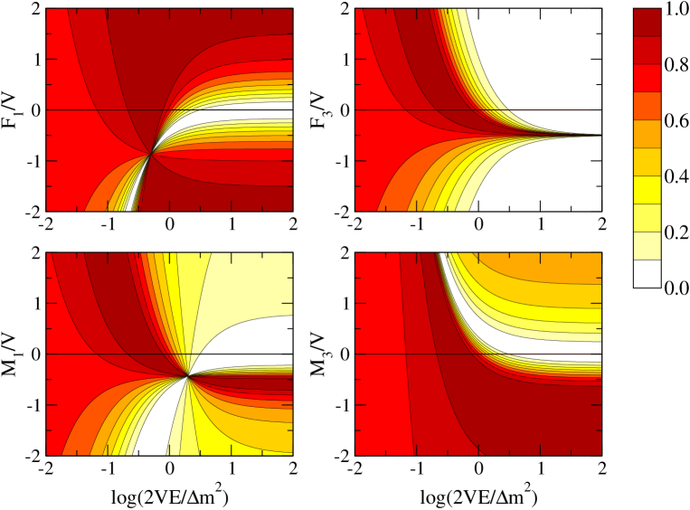
In Fig. 2, we plot the possible range of as a function of , where , is the matter potential, and . For comparison, a neutrino factory with a neutrino energy of GeV and a matter density of 3 g/cm3 will have MeV2 and the position at which we need to consider the possible range of then depends on the bounds on the non-standard parameters . In general, the bounds for depend on the type of non-standard effect and the types of interactions that are considered. In the case of NSI, it is common to write the non-standard interaction parameters as
| (28) |
where we sum over different types of fermions, depends on the non-standard interaction with the fermion , and is the number density of the fermion . In addition, is often split into , where and denotes the projector used in the fermion factor of the effective non-standard Lagrangian density, i.e.,
| (29) |
Recent bounds for can be found in Ref. [54] for electron neutrino interactions with electrons (i.e., ) and Ref. [55] for interactions with first generation Standard Model fermions. As an example, the bounds from Ref. [54] for the (which is considered in Fig. 2) are
| (30) |
respectively. This means that the bounds, especially in this sector, are weak, which we will use in the next section. From Fig. 2, we can deduce that the off-diagonal terms have a larger potential of altering the value of than the diagonal terms, the maximal value can even exceed , corresponding to . In addition, it is possible to suppress the effective to zero if introducing non-standard effects. It follows that a relatively large signal, bounded only by the size of the non-standard effects, can be induced or that a large signal can be suppressed by non-standard effects. Note that the effects quickly disappear at low energies, e.g., in reactor experiments. In order to tell a genuine signal apart from a signal induced by non-standard interactions, it is necessary to study the actual distortion of the energy spectrum induced by the neutrino oscillations.
5 A numerical example: Neutrino factory for large
This section is not supposed to be a complete study of non-standard Hamiltonian effects, but to demonstrate some of the qualitatively discussed properties from the last sections in a complete numerical simulation of a possible future experiment using the exact three-flavor probabilities. Therefore, we have to make a number of assumptions. We use a modified version of the GLoBES software [56] to include non-standard effects. As a future high-precision instrument, we choose the neutrino factory experiment setup from Refs. [57, 58] with , a magnetized iron calorimeter detector, useful muon decays per year, and four years of running time in each polarity.666Compared to Ref. [57], we use a 2.5 % systematic normalization error for all channels as in Ref. [58]. This experiment uses muon neutrino disappearance and electron to muon neutrino appearance as oscillation channels for both neutrinos and antineutrinos (in the muon and anti-muon operation modes combined). For the neutrino oscillation parameters, we use , , , and [59, 60, 61, 62], as well as we assume a 5 % external measurement for and [60] and include matter density uncertainties of the order of 5 % [63, 64]. In order to test precision measurements of the non-standard effects, we use close to the CHOOZ upper bound777In general, a large will imply a large signal in the appearance channel. However, non-zero effective could arise even if , cf., Fig. 2. For effects which are diagonal in flavor basis, a large would be preferred in order to make an observation of the non-standard effect. We have used large as an example, since one may argue that the finding of new effects at present experiments (such as MINOS) may lead to a good reason for constructing a neutrino factory. One should also observe that, in principle, it would be possible to find non-standard effects at, e.g., MINOS [65, 66]. However, the precision of a neutrino factory would be more sensitive to small effects, and thus, more useful for distinguishing between effects. [67], as well as we assume a normal mass hierarchy and . For simplicity, we do not take the -degeneracy [68] into account, but we include the intrinsic -degeneracy [69], whereas the octant degeneracy does not appear for maximal mixing [70]. Note that we do not include external bounds on the non-standard physics and , which, for instance, mean that we allow “fake” solutions of above the CHOOZ bound. This assumption is plausible, since, depending on the effect, the CHOOZ bound may have been affected by the non-standard effect as well.
5.1 Test model
Since we choose to be large, let us first of all focus on the appearance channel of oscillating into (or oscillating into ). Expanding in small and , we have for (which should be a good approximation for ) [71, 72, 73]
| (31) |
where and . Similarly, is described by this equation with replaced by . This means that we may be effectively dealing with the two-flavor limits described in Sec. 3, depending on the degree the non-standard effects are different for the and flavors (cf., Appendix C).
Using the parameterization in Eqs. (5) and (6) applied to the 1-3-sector, we therefore adopt the following Hamiltonian:
| (35) | |||||
| (39) |
In this model, and correspond to the CP conserving and CP violating parts of a mass-changing effect, whereas is a mass-conserving effect. In addition, and are the CP conserving and CP violating parts of a flavor-changing effect, whereas is a flavor-conserving effect. As motivated before, it is plausible to assume that one of these non-standard effects may be dominating the other ones, because many models predict such a dominating component and the experimental constraints on some quantities are rather strong. In addition, Eq. (39) implies that the effects are mainly present in the 1-3-sector, which can be motivated by rather weak experimental bounds on the -sector. For example, the bounds on the matrix element are rather weak in the case of NSI, making it viable that this term is dominating the NSI Hamiltonian. In this case, we obtain
| (40) |
Thus, we have a flavor violating effect with representing the CP conserving part of the NSI and representing the CP violating part of the NSI. The form of the mass effects has been chosen to match the expected energy dependence of MVN in order to discuss effects with realistic spectral (energy) dependencies.
Note that the parameterization in Eq. (39) does not exactly correspond to the two-flavor limit even for , since there are some non-trivial mixing effects in the 2-3-sector as described in Appendix C. This parameterization is also obviously not the whole story in the three-flavor scenario. For instance, we assume the same sign for effects on neutrinos and antineutrinos, which may, depending on the model, not apply in general. However, we will demonstrate some of the characteristics from Sec. 3.2 with this approach. In addition, note that we have now adopted a specific energy dependence of the flavor and mass effects, where the definition of the energy dependence in the ’s is slightly different from the one in the ’s in Sec. 2, i.e., . In this case, the mass effects could be coming from MVN changing the mass eigenstates, whereas the flavor effects correspond to some NSI approximately constant in the considered energy range. We will quantify the size of the and in terms of the normalized quantities (for ) and (for ). This quantification makes sense, since it is obvious from Eq. (39) that the effect of these quantities will have to be compared with the order of and , respectively. Note that from Sec. 4, which means that it will be interesting to compare the precisions of and to the current bounds for . Furthermore, note that the mass effects can be simply rotated away by a different choice of the mixing matrix and the mass squared differences because of the same energy dependence in this example. However, since we assume the solar parameters to be measured externally, we will observe that constraints to the can be derived. Such an external measurement with a similar environment dependence to the neutrino factory comes from KamLAND, which turns out to be very consistent with the ones from solar neutrino experiments. Since most non-standard effects in oscillations are dependent on the matter density (such as MVNs with acceleron couplings to matter fields, or non-standard flavor-changing matter effects generated by higher-dimensional operators), it is plausible to assume that strong constraints hold for the solar sector because of the very different environments/densities within the Sun and the Earth.
5.2 Identifying specific pure effects
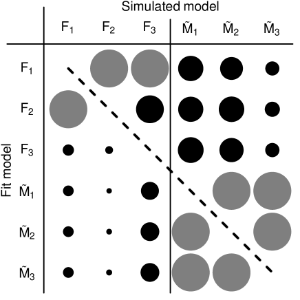
If we discover a non-standard effect, it will be an interesting question how easily it can be identified. Assuming one dominating effect of the mass or flavor type, which we have introduced as “pure effect”, we want to know how well it can be distinguished from other such effects of different qualitative nature. Therefore, in Fig. 3, we show the correlation between simulated and fit pure effects. For this figure, we simulate a pure effect (column) and fit it with a different one (row), i.e., we marginalize over the respective or . The areas of the disks are proportional to the minimum simulated value necessary to establish a effect, where we have chosen a cutoff of and (corresponding to the largest gray disks).888Note that, for instance, the gray disks for and correspond to the order of magnitude of the upper bounds in Eq. (30), which means that testing considerably larger effects does not make sense. This means that the size of the disks measures the correlation between two pure effects and the ability to discriminate those.
One can easily make a number of qualitative observations from Sec. 3.2 quantitative. First, it is hard to discriminate between and (CP conserving and CP violating flavor-changing effects), since these effects are qualitatively similar and highly correlated with (as we have tested). However, if Nature implemented a flavor-changing or effect, then one could easily establish it against and the pure mass effects. In general, note that a discrimination between flavor and mass effects is rather easy because of their different spectral dependence in this example (such as between and ). The difference to can be explained by the different flavor-conserving nature of . The results look somewhat different for the column: Because of the correlation with and all of the neutrino oscillation parameters (see below), it will be hard to establish this effect. For the simulated mass effects, the scale is different, i.e., one cannot directly compare the -columns with the -columns. Again, the mass effects can be distinguished from the pure flavor effects to some extent. However, it is quite impossible to establish a mass effect against another one, since they can be easily simulated by a different set of mass squared differences and mixing parameters with the same energy dependence. The only reason why the pure mass effects can be established in this example at all is that we have imposed external constraints on the solar parameters as motivated above.
5.3 Discovery of non-standard physics and potential for improvements
| Quantity | Lower limit () | Upper limit () | Lower limit () | Upper limit () |
|---|---|---|---|---|
| 0.008 | 0.008 | 0.025 | 0.026 | |
| 0.003 | 0.003 | 0.008 | 0.008 | |
| 0.016 | 0.016 | 0.049 | 0.082 | |
| 0.176 | 0.118 | 0.218 | 0.211 | |
| 0.105 | 0.126 | 0.181 | 0.212 | |
| 0.015 | 0.015 | 0.044 | 0.090 |
A very important issue of any pure non-standard effect is its evidence compared to the standard three-flavor oscillation scenario. Therefore, in Table 1, we show the discovery reaches for the parameters from Eq. (39) against the standard three-flavor neutrino oscillation scenario. This means that the shown pure effects are simulated and the standard three-flavor neutrino oscillation parameters are marginalized over. Comparing the precisions of and with the numbers in Eq. (30) is impressive. However, these discovery reaches depend on (and ) and we have assumed a very large (and ). Note that the reach in is actually better than the one in , which is different from what is found in the two-flavor limit in Sec. 3.2. The reasons are the mixing effects in the 2-3-sector and that is a non-trivial source of CP violation in the three-flavor case.
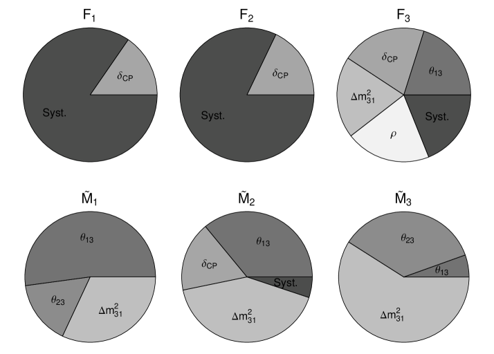
Except from these sensitivities, which somewhat depend on the specific model, the behavior for neutrinos and antineutrinos, and so on, it may be of some interest to obtain hints how these reaches can be improved. In order to study this aspect, we show the so-called “impact factors” for the test of specific simulated models against standard three-flavor neutrino oscillations in Fig. 4. These impact factors test the relative impact of the measurement errors on the neutrino oscillation parameters and systematics. In order to compute them, the non-standard discovery limits are evaluated with all neutrino oscillation parameters marginalized over, matter density uncertainties included, and systematics switched on (standard). In addition, in order to test a specific impact factor, one neutrino oscillation parameter is fixed at one time (or systematics is switched off), and the corresponding discovery reach for the non-standard effect is compared to the discovery reach including all uncertainties and systematics. The difference between these to discovery reaches describes the impact of a particular measurement error (or systematics), and the relative impact in Fig. 4 quantifies what one needs to optimize for in order to improve the discovery reach. For example, for (lower right pie), the error on is the main impact factor in our model, which needs to be improved to increase the discovery reach.
Again, a number of aspects from Sec. 3.2 can be verified. For and effects, systematics is the main impact factor, since these flavor effects determine the overall height of the appearance signal and are not introduced with a specific spectral dependence (remember that we use a conservative overall normalization error of 2.5 %). For effects, we have earlier determined the matter density uncertainty as an important constraint. However, improving the knowledge on , , or does have a similar effect, since the extraction of the individual parameters becomes easier. For the mass effects, we encounter a completely different behavior. Remember that we have defined the mass effects with the same energy dependence as the mass squared differences, which means that particularly is easily mixed up with . On the other hand, and are related to a flavor change in the appearance channel via the mixing matrix, i.e., the leptonic mixing angle . Therefore, it is not surprising that such a flavor change can be interpreted as either a mixing or a mass-changing effect. Compared to Sec. 3.2, there are also a number of differences coming from the three-flavor treatment (solar and CP effects) and the mixing in the 2-3-sector. These effects introduce additional correlations with and . However, they are also the reason why, for example, can be constrained at all from this experiment alone [in the pure two-flavor case or without external constraints on the solar parameters, it would be impossible to distinguish between a non-vanishing and a different if the mass effects had the energy dependence assumed in Eq. (39)].
5.4 Comparison to damping effects
In the context of the non-standard effect identification, a more general question is the ability to distinguish Hamiltonian effects and effects on probability level. The probability level effects lead to damping of the neutrino oscillation probabilities (“damping effects”) and were studied in detail in Ref. [1]. They may originate from decoherence, neutrino decay, or other physics mechanisms. In this section, we address this identification in somewhat more detail in a qualitative manner. A relatively new ingredient for this identification is the use of the “Silver” () channel at a neutrino factory [74, 75]. It has been noticed [28, 65, 66] that the Silver channel probability can be greatly enhanced for non-standard Hamiltonian effects. This corresponds to what we have found in Sec. 3.2, i.e., the Silver channel, which is similar to the “Golden” () channel when there are no non-standard effects, behaves as our two-flavor limit in Sec. 3.2 for large energies.
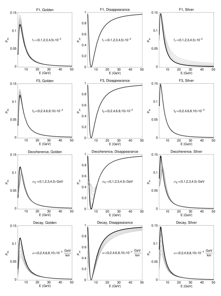
In Fig. 5, we show the impact of different types of effects on the neutrino oscillation probabilities in the Golden channel , the disappearance channel 999The probability is actually the survival probability. However, this is the relevant probability when searching for disappearance rather than the disappearance probability ., and the Silver channel (shown in columns) at a possible future neutrino factory (relevant energy range shown). The different rows correspond to scenarios with (flavor-changing without CP violation, Hamiltonian-level), (flavor-conserving, Hamiltonian-level), decoherence, and neutrino decay, respectively. The different model parameters for the different curves are given in the individual plots, where the thick curves correspond to the standard neutrino oscillation scenario. For a description of the decoherence and decay models, see Ref. [1]. In short, the decoherence model corresponds to standard wave packet decoherence, whereas the decay model assumes equal decay rates for all mass eigenstates (which can, for instance, be motivated by a degenerate mass spectrum). Note that this figure is shown for neutrinos only and that the comparison between the neutrino and antineutrino behavior can provide information on the underlying physics as well. However, this behavior is model-dependent.
Figure 5 is very useful to study the characteristics of different effects and to illustrate how the information from different neutrino oscillation channels can be used to disentangle them. First, it is important to note that it is difficult to construct a damping effect without large impact on the disappearance channel. Since the event rates in this channel are very high, it is probably the first place to look for non-standard physics. In addition, damping effects tend to suppress the Golden and Silver channel probabilities around the oscillation peak, which can, depending on the model, be very different for Hamiltonian-level effects. However, as it can be read off from Fig. 5, Hamiltonian-level effects produce, similar to , the largest effect in the appearance channels.101010The weak influence of the non-standard Hamiltonian level effects on the disappearance probability is purely due to the fact that Eq. (39) has been assumed for the non-standard Hamiltonian, where we have assumed the states to be unaffected. However, as mentioned earlier, there are also stronger bounds on any NSI involving . In particular, the flavor-conserving effect may enhance the silver probability as demonstrated in the two-flavor limit in Sec. 3.2. Comparing all panels in Fig. 5, we expect that the combination of all channels serves as a good model discriminator because each of the shown models has a unique signature if all these channels are combined. For example, we have tested that adding a OPERA-like emulsion cloud chamber for the silver channel at the same baseline as the golden channel improves the discovery reach by about 60 % (for simulation details, see Ref. [76]) because of the silver channel signature at large energies. Therefore, we believe that this combination of different channels in combination with precise oscillation parameter measurements and spectral signatures can reveal non-standard physics.
6 Summary and conclusions
For future long-baseline neutrino oscillation precision measurements, such as neutrino factories, it will be an important question how to identify a non-standard effect. While it is very likely that many theoretical models will fit such a “new physics” discovery, the classification of models corresponding to this discovery from a phenomenological point of view will be very important for the planning of the following generation of experiments. Hence, there is strong interest in a top-down approach to non-standard physics tests, since the impact of future measurements on theory has to be assessed to promote the experiment. So far, mainly the bottom-up approach has been used, which is testing specific models in an experiment. Therefore, it has been one of the main goals of this work to demonstrate the identification and separation of individual phenomenological classes by generic arguments.
In summary, we have studied non-standard effects on neutrino oscillations on the Hamiltonian level. We have parameterized these effects in terms of the generators of the Lie algebra, and we have introduced them in flavor (such as coming from FCNC or NSI) and mass (such as coming from MVN) bases. As a trivial fact, there is, in principle, no mathematical difference between these effects if one allows the most general form in each basis. Given the detection of a general non-standard effect on Hamiltonian level, it is therefore not possible to classify it as a flavor or mass effect without further assumptions or knowledge and, from an empirical point of view, the classification is a matter of definition. Therefore, we have defined “pure” effects as effects which are proportional to specific individual generators. Those correspond to pure flavor/mass conserving/violating effects, i.e., effects which affect particular flavor or mass eigenstates. This definition makes sense if one assumes that the underlying theoretical model causes one dominating non-standard effect. It is then the simplicity of the form in the respective basis which defines the effect to be of flavor or mass type. Therefore, the concept of these pure effects allows the choice of the most “natural” class of models for further testing, which is most appealing from the physics point of view.
From the analytical point of view, we have studied the effects in the two-flavor limit. We have derived the modified mass squared differences and mixing angles (parameter mappings) as well as the modified resonance conditions including standard matter effects. In addition, we have discussed the application of this two-flavor limit to experiments, in particular, to the neutrino oscillation probability . This probability can be described to a first approximation by a two-flavor limit for large , where the -term dominates the CP effects. In addition, non-standard effects in the 1-3-sector have so far very poor limits (such as ) and the driving parameter is unknown, which means that there is room for confusion between and non-standard effects (see, e.g., Ref. [26, 27]). We have found that there are several generic features for different types of effects. While any flavor violating pure effect can obviously change the transition probabilities, it does not affect the resonance condition/energy. However, a flavor conserving pure effect changes the resonance condition similar to matter effects and is highly correlated with the matter density. In addition, it can suppress the flavor transition for large energies similar to matter effects – even in vacuum. Pure mass effects behave, in principle, as rotations of the flavor effects by the mixing angles, i.e., a pure mass effect will be observed as a linear combination of flavor effects. However, for a pure mass conserving effect, these flavor effects combine with special characteristics, since the mass effect is similar to an (energy dependent) change of the vacuum mass squared difference, i.e., it basically squeezes or stretches the oscillation pattern. Since in quantum field theory any non-standard effect may originate in the coherent (Hamiltonian effect) or incoherent (“damping” effect) summation of amplitudes, we have compared the non-standard Hamiltonian effects to the previously studied “damping” effects on probability level. We have found that these two classes can be distinguished by typical characteristics. Non-standard Hamiltonian effects shift the oscillation pattern, while “damping” effects, in general, do not. In principle, the different classes of non-standard Hamiltonian effects can be identified by their modification of oscillation amplitudes for large energies, the shift of the matter resonance, the comparison of different -ranges, etc.
We have also studied some aspects of the three-flavor generalization of general non-standard Hamiltonian effects using perturbation theory as well as numeric calculations. By assuming small non-standard Hamiltonian effects, we have derived expressions for the effective matrix elements using perturbation theory and observed how the confusion theorem between and non-standard effects described in Ref. [27] arises at the Hamiltonian level. Our numeric calculations show that non-standard effects can alter the determination of significantly at higher energies, while still preserving a high accuracy at lower energies (cf., Fig. 2).
Eventually, we have demonstrated, at a numerical example for a neutrino factory, that many of these features can be found in a realistic experimental simulation using three flavors and specific spectral (energy) dependencies for the non-standard effects. For example, while it is simple to distinguish a flavor changing effect from flavor conserving or mass effects in general, mass effects are hard to establish as long as the neutrino oscillation parameters are not known from an independent source (such as with a different matter density for MVN). In addition, we have compared the obtainable discovery reaches for to the current limits, and we have found at least an order of magnitude improvement for large and . We have also compared the Hamiltonian level effects to damping effects and found that they can be distinguished by their specific alteration of the spectra in different neutrino oscillation channels.
Since the past has told us that neutrinos are good for surprises, the high precision measurements at future neutrino oscillation experiments might as well reveal a detection of “new physics” beyond the Standard Model (extended to include massive neutrinos). Therefore, we conclude that one should include general strategies to look for non-standard effects in future neutrino oscillation experiments, where we have followed a top-down approach: Instead of testing particular models (bottom-up), we have assumed that some inconsistency will be found first. Secondly, one may want to classify this inconsistency to be either a Hamiltonian or a probability level (“damping”) effect. Finally, individual models are identified which fit this effect. Since we do not know exactly what we are looking for, such an approach might be a clever search strategy, and it can be useful to promote an experiment as a discriminator among different classes of theoretical models. Future studies should demonstrate how such an approach can be most efficiently extended to three neutrino flavors, which neutrino oscillation channels are most suitable, and what the correlations with the existing fundamental neutrino oscillation parameters imply.
Acknowledgments
W.W. would like to thank the Theoretical Elementary Particle Physics group at KTH for the warm hospitality during a research visit. In addition, T.O. and W.W. would like to thank Manfred Lindner and his group at TUM in Munich for the warm hospitality during their research visits where parts of this paper were developed.
This work was supported by the Royal Swedish Academy of Sciences (KVA), the Swedish Research Council (Vetenskapsrådet), Contract Nos. 621-2001-1611, 621-2002-3577, the Göran Gustafsson Foundation, the Magnus Bergvall Foundation, the W. M. Keck Foundation, and NSF grant PHY-0070928.
Appendix A General formalism for the two-flavor scenario
Any two-flavor Hamiltonian can be written in flavor basis on the form
| (41) |
where and is the vector of the three Pauli matrices (cf., the pictorial description of two-flavor neutrino oscillations in Ref. [77]). For a time-independent Hamiltonian, the time evolution operator is given by
| (42) |
Using the relation , one obtains
| (43) |
where is the unit matrix. This gives the two-flavor neutrino oscillation probabilities of the form
| (44) | ||||
| (45) |
where
Here the ’s are the components of the Hamiltonian and is the effective mixing angle.
In the standard two-flavor neutrino oscillation scenario, , , and . In general, the resonance condition, i.e., the condition for maximal effective mixing, is . The Hamiltonian is represented as a vector in , the third direction being the “flavor” eigendirection. The mixing is given by the angle between the Hamiltonian vector and the flavor eigendirection. The mixing is maximal, i.e., , when the Hamiltonian vector is orthogonal to the flavor eigendirection, which, as expected, is equivalent to the resonance condition.
The flavor and mass bases, and thus, the flavor and mass effects, are intimately associated with each other. For the case of , i.e., for two neutrino flavors, any effective contribution to the Hamiltonian can be written in either flavor or mass basis, i.e., as or . Since the effect must be the same regardless of the basis it is expressed in, we obtain the relations
| (46) |
from Eq. (7), i.e., one obtains and by rotating and by the angle as well as one has . Thus, the transformation in Eq. (46) relates flavor and mass effects and shows that they are linear combinations of each other.
Appendix B Non-standard effects for large mixing
In this appendix, we concentrate on pure effects in the limit of large mixing. When the mixing goes to maximal, we have . This means that the resonance condition in Eq. (12) cannot be fulfilled for (i.e., “matter resonance”) at reasonably large energies.111111Note that, in this appendix, we assume that matter effects determine the resonance energy and the non-standard effects are sub-leading contributions, which may shift the resonance energy. Thus, we refer to the “matter resonance” as the resonance condition in Eq. (12) for . From Eq. (10), we can easily observe that and will not modify at all in the absence of matter (and ) effects (for example, in or a vacuum probability). Independent of matter effects, can increase the suppression of for large energies. If the resonance condition in Eq. (12) is fulfilled, then will be independent of and . However, in the presence of matter effects (such as for in the limit ), and can reduce the matter effect suppression of for large energies (cf., Fig. 6), i.e., they can increase the effective mixing. Eventually, it is obvious from Eqs. (9) and (11) that the oscillation frequency is always increased for positive ’s.
It can also be interesting (and quite illuminating) to study how different pure (flavor or mass) effects affect the effective neutrino mixing and oscillations. In Fig. 6, we plot the effective mixing resulting from “pure” flavor and mass effects.
From this figure, some features become quite apparent, e.g., some generic features are the shift in the resonance energy for , , and , the non-zero high-energy mixing for all effects but the flavor conserving effect , and the appearance of an anti-resonance – where goes to zero for some finite energy – for , , and .
The shift in the resonance energy is simply due to the shift in the -component of the total effective Hamiltonian in flavor basis (as was mentioned earlier, the resonance condition is ). The fact that there is no shift of the resonance condition for and was also discussed earlier.
The reason why the effective high-energy mixing generally turns out to be non-zero is also quite easy to realize. At high energies, the effective matter potential, which is diagonal in flavor basis, dominates over the vacuum Hamiltonian. As a result, the effective mixing is usually zero at high energies. However, if there is a non-standard effect with a corresponding effective addition to the Hamiltonian which is non-diagonal and is either constant or increasing with energy, then the effective mixing at high energies will be fully determined by the ratio of the non-standard effect and the matter potential.
The anti-resonance appears when in flavor basis. Since in the standard neutrino oscillation scenario, it is apparent that this anti-resonance will occur for some value of . In addition, since and are linear combinations of and , the anti-resonance will also appear for and effects, as can be seen from the plots in Fig. 6.
There are also some interesting features that are specific for different effects. First, for effects, we note that the resonance condition is unchanged and that the mixing is constant as a function of energy for (the reason for this is that the sum of the non-standard Hamiltonian and the matter potential is proportional to the vacuum Hamiltonian). Then, for flavor conserving effects, we note that these correspond to changes in the effective matter potential. For , we obtain an effective matter potential which is negative, resulting in a disappearance of the resonance. Next, for effects, the mixing is constant when , in analogy with the effects (again, the reason is that the sum of the non-standard Hamiltonian and the matter potential is proportional to the vacuum Hamiltonian). Also in analogy with the effects is that there is a value of , where the mixing does not depend on the ratio. However, in the case of effects, this is not the resonance mixing, but rather a mixing of , which appears at . Finally, for mass conserving effects, we note that the resonance disappears when .
The reason why the equivalent and effects are not included is that these effects always lead to an increase in the effective mixing angle for all energies, and thus, those plots do not show as many interesting features as the plots included. In addition, we note that if the non-standard effects are energy dependent, then the effective mixing will be given by the mixing along some non-constant function of in Fig. 6.
Appendix C Two-flavor limits of three flavor scenarios
In this appendix, we discuss subtleties with the definition of the effective two-flavor scenarios introduced in Sec. 3.2. Remember that the effective two-flavor neutrino oscillation scenarios should be defined in terms of the effective two-flavor sector in question. For example, in the limit when , the effective two-flavor sector is spanned by and . Thus, the limit can be considered as an exact pure two-flavor scenario only if the non-standard effects preserve the two-flavor limit (i.e., no off-diagonal terms mixing and with the remaining neutrino state ). If the non-standard addition to the Hamiltonian is given by
| (47) |
then the corresponding addition in the basis spanned by is
| (48) |
where
From this relation, we deduce that the limit will be a pure two-flavor case if for all non-standard effects which do not involve and (which could be implemented by, e.g., and ). In general, some of the conclusions for the two-flavor case will therefore not apply to three flavors. We have, in the numerical example in Sec. 5, demonstrated which of the conclusions that do hold. The case when is similar to the case described above, with the exception that the effective two-flavor sector is now spanned by and instead of and . For the limit and , there is no subtlety and the two-flavor sector is spanned by and .
References
- [1] M. Blennow, T. Ohlsson, and W. Winter, JHEP 06, 049 (2005), hep-ph/0502147.
- [2] H. Päs, S. Pakvasa, and T. J. Weiler, Phys. Rev. D72, 095017 (2005), hep-ph/0504096.
- [3] J. W. F. Valle, Phys. Lett. B199, 432 (1987).
- [4] J. W. F. Valle, J. Phys. G29, 1819 (2003), and references therein.
- [5] S. Bergmann, Nucl. Phys. B515, 363 (1998), hep-ph/9707398.
- [6] S. Bergmann and A. Kagan, Nucl. Phys. B538, 368 (1999), hep-ph/9803305.
- [7] S. Bergmann, Y. Grossman, and E. Nardi, Phys. Rev. D60, 093008 (1999), hep-ph/9903517.
- [8] L. Wolfenstein, Phys. Rev. D17, 2369 (1978).
- [9] P. I. Krastev and J. N. Bahcall (1997), hep-ph/9703267.
- [10] S. Bergmann, M. M. Guzzo, P. C. de Holanda, P. I. Krastev, and H. Nunokawa, Phys. Rev. D62, 073001 (2000), hep-ph/0004049.
- [11] M. Guzzo et al., Nucl. Phys. B629, 479 (2002), hep-ph/0112310.
- [12] A. Friedland, C. Lunardini, and C. Peña-Garay, Phys. Lett. B594, 347 (2004), hep-ph/0402266.
- [13] O. G. Miranda, M. A. Tórtola, and J. W. F. Valle (2004), hep-ph/0406280.
- [14] S. Bergmann, Y. Grossman, and D. M. Pierce, Phys. Rev. D61, 053005 (2000), hep-ph/9909390.
- [15] N. Fornengo, M. Maltoni, R. Tomàs Bayo, and J. W. F. Valle, Phys. Rev. D65, 013010 (2002), hep-ph/0108043.
- [16] M. C. Gonzalez-Garcia and M. Maltoni, Phys. Rev. D70, 033010 (2004), hep-ph/0404085.
- [17] A. Friedland, C. Lunardini, and M. Maltoni, Phys. Rev. D70, 111301 (2004), hep-ph/0408264.
- [18] A. Friedland and C. Lunardini (2005), hep-ph/0506143.
- [19] G. L. Fogli, E. Lisi, A. Mirizzi, and D. Montanino, Phys. Rev. D66, 013009 (2002), hep-ph/0202269.
- [20] B. Bekman, J. Gluza, J. Holeczek, J. Syska, and M. Zrałek, Phys. Rev. D66, 093004 (2002), hep-ph/0207015.
- [21] S. Bergmann and Y. Grossman, Phys. Rev. D59, 093005 (1999), hep-ph/9809524.
- [22] T. Ota and J. Sato, Phys. Lett. B545, 367 (2002), hep-ph/0202145.
- [23] T. Ota, J. Sato, and N.-a. Yamashita, Phys. Rev. D65, 093015 (2002), hep-ph/0112329.
- [24] M. C. Gonzalez-Garcia, Y. Grossman, A. Gusso, and Y. Nir, Phys. Rev. D64, 096006 (2001), hep-ph/0105159.
- [25] P. Huber and J. W. F. Valle, Phys. Lett. B523, 151 (2001), hep-ph/0108193.
- [26] P. Huber, T. Schwetz, and J. W. F. Valle, Phys. Rev. Lett. 88, 101804 (2002), hep-ph/0111224.
- [27] P. Huber, T. Schwetz, and J. W. F. Valle, Phys. Rev. D66, 013006 (2002), hep-ph/0202048.
- [28] M. Campanelli and A. Romanino, Phys. Rev. D66, 113001 (2002), hep-ph/0207350.
- [29] P. Gu, X. Wang, and X. Zhang, Phys. Rev. D68, 087301 (2003), hep-ph/0307148.
- [30] R. Fardon, A. E. Nelson, and N. Weiner, JCAP 0410, 005 (2004), astro-ph/0309800.
- [31] V. Barger, P. Huber, and D. Marfatia (2005), hep-ph/0502196.
- [32] M. Cirelli, M. C. Gonzalez-Garcia, and C. Peña-Garay, Nucl. Phys. B719, 219 (2005), hep-ph/0503028.
- [33] X.-J. Bi, P.-h. Gu, X.-l. Wang, and X.-m. Zhang, Phys. Rev. D69, 113007 (2004), hep-ph/0311022.
- [34] P. Q. Hung and H. Päs, Mod. Phys. Lett. A20, 1209 (2005), astro-ph/0311131.
- [35] D. B. Kaplan, A. E. Nelson, and N. Weiner, Phys. Rev. Lett. 93, 091801 (2004), hep-ph/0401099.
- [36] P.-h. Gu and X.-j. Bi, Phys. Rev. D70, 063511 (2004), hep-ph/0405092.
- [37] K. M. Zurek, JHEP 10, 058 (2004), hep-ph/0405141.
- [38] R. D. Peccei, Phys. Rev. D71, 023527 (2005), hep-ph/0411137.
- [39] H. Li, Z.-g. Dai, and X.-m. Zhang, Phys. Rev. D71, 113003 (2005), hep-ph/0411228.
- [40] X.-J. Bi, B. Feng, H. Li, and X.-m. Zhang (2004), hep-ph/0412002.
- [41] R. Horvat (2005), astro-ph/0505507.
- [42] N. Afshordi, M. Zaldarriaga, and K. Kohri (2005), astro-ph/0506663.
- [43] R. Takahashi and M. Tanimoto (2005), hep-ph/0507142.
- [44] R. Fardon, A. E. Nelson, and N. Weiner (2005), hep-ph/0507235.
- [45] A. W. Brookfield, C. van de Bruck, D. F. Mota, and D. Tocchini-Valentini, Phys. Rev. Lett. 96, 061301 (2006), astro-ph/0503349.
- [46] M. Kawasaki, H. Murayama, and T. Yanagida, Mod. Phys. Lett. A7, 563 (1992).
- [47] G. J. Stephenson Jr., T. Goldman, and B. H. J. McKellar, Int. J. Mod. Phys. A13, 2765 (1998), hep-ph/9603392.
- [48] G. J. Stephenson Jr., T. Goldman, and B. H. J. McKellar, Mod. Phys. Lett. A12, 2391 (1997), hep-ph/9610317.
- [49] R. F. Sawyer, Phys. Lett. B448, 174 (1999), hep-ph/9809348.
- [50] S. P. Mikheyev and A. Y. Smirnov, Sov. J. Nucl. Phys. 42, 913 (1985).
- [51] S. P. Mikheyev and A. Y. Smirnov, Nuovo Cim. C9, 17 (1986).
- [52] E. K. Akhmedov, R. Johansson, M. Lindner, T. Ohlsson, and T. Schwetz, JHEP 04, 078 (2004), hep-ph/0402175.
- [53] T. Schwetz and W. Winter, Phys. Lett. B633, 557 (2006), hep-ph/0511177.
- [54] J. Barranco, O. G. Miranda, C. A. Moura, and J. W. F. Valle (2005), hep-ph/0512195.
- [55] S. Davidson, C. Peña-Garay, N. Rius, and A. Santamaria, JHEP 03, 011 (2003), hep-ph/0302093.
- [56] P. Huber, M. Lindner, and W. Winter, Comput. Phys. Commun. 167, 195 (2005), hep-ph/0407333.
- [57] P. Huber, M. Lindner, and W. Winter, Nucl. Phys. B645, 3 (2002), hep-ph/0204352.
- [58] P. Huber, M. Lindner, M. Rolinec, and W. Winter, Phys. Rev. D73, 053002 (2006), hep-ph/0506237.
- [59] G. L. Fogli, E. Lisi, A. Marrone, and D. Montanino, Phys. Rev. D67, 093006 (2003), hep-ph/0303064.
- [60] J. N. Bahcall, M. C. Gonzalez-Garcia, and C. Peña-Garay, JHEP 08, 016 (2004), hep-ph/0406294.
- [61] A. Bandyopadhyay, S. Choubey, S. Goswami, S. T. Petcov, and D. P. Roy (2004), hep-ph/0406328.
- [62] M. Maltoni, T. Schwetz, M. A. Tórtola, and J. W. F. Valle, New J. Phys. 6, 122 (2004), hep-ph/0405172.
- [63] R. J. Geller and T. Hara, Phys. Rev. Lett. 49, 98 (2001), hep-ph/0111342.
- [64] T. Ohlsson and W. Winter, Phys. Rev. D68, 073007 (2003), hep-ph/0307178.
- [65] N. Kitazawa, H. Sugiyama, and O. Yasuda (2006), hep-ph/0606013.
- [66] A. Friedland and C. Lunardini, Phys. Rev. D74, 033012 (2006), hep-ph/0606101.
- [67] M. Apollonio et al. (CHOOZ), Phys. Lett. B466, 415 (1999), hep-ex/9907037.
- [68] H. Minakata and H. Nunokawa, JHEP 10, 001 (2001), hep-ph/0108085.
- [69] J. Burguet-Castell, M. B. Gavela, J. J. Gomez-Cadenas, P. Hernandez, and O. Mena, Nucl. Phys. B608, 301 (2001), hep-ph/0103258.
- [70] G. L. Fogli and E. Lisi, Phys. Rev. D54, 3667 (1996), hep-ph/9604415.
- [71] A. Cervera et al., Nucl. Phys. B579, 17 (2000), hep-ph/0002108.
- [72] M. Freund, P. Huber, and M. Lindner, Nucl. Phys. B585, 105 (2000), hep-ph/0004085.
- [73] M. Freund, Phys. Rev. D64, 053003 (2001), hep-ph/0103300.
- [74] A. Donini, D. Meloni, and P. Migliozzi, Nucl. Phys. B646, 321 (2002), hep-ph/0206034.
- [75] D. Autiero et al., Eur. Phys. J. C33, 243 (2004), hep-ph/0305185.
- [76] P. Huber, M. Lindner, M. Rolinec, and W. Winter (2006), hep-ph/0606119.
- [77] C. W. Kim and A. Pevsner Chur, Switzerland: Harwood (1993) 429 p. (Contemporary concepts in physics, 8).