2005 International Linear Collider Workshop - Stanford, U.S.A.
Probing Electroweak Top Quark Couplings at Hadron and Lepton Colliders

Abstract

The International Linear Collider (ILC) will be able to precisely measure the electroweak couplings of the top in $e^{+}e^{-}\to t\bar{t}$. We compare the limits which can be achieved at the ILC with those which can be obtained in $t\bar{t}\gamma$ and $t\bar{t}Z$ production at the Large Hadron Collider (LHC).

I INTRODUCTION

Although the top quark was discovered almost ten years ago topcdf ; topd0 , many of its properties are still only poorly known Chakraborty:2003iw . In particular, the couplings of the top quark to the electroweak (EW) gauge bosons have not yet been directly measured. Current data provide only weak constraints on the couplings of the top quark with the EW gauge bosons, except for the $ttZ$ vector and axial vector couplings which are rather tightly but indirectly constrained by LEP data; and the right-handed $tbW$ coupling, which is severely bound by the observed $b\to s\gamma$ rate Larios:1999au .

At an $e^{+}e^{-}$ linear collider with $\sqrt{s}=500$ GeV and an integrated luminosity of $100-200$ fb^-1 one can hope to measure the $ttV$ ($V=\gamma,\,Z$) couplings in top pair production with a few-percent precision Abe:2001nq . However, the process $e^{+}e^{-}\to\gamma^{*}/Z\to t\bar{t}$ is sensitive to both $tt\gamma$ and $ttZ$ couplings and significant cancellations between the various couplings can occur. At hadron colliders, $t\bar{t}$ production is so dominated by the QCD processes $q\bar{q}\to g^{*}\to t\bar{t}$ and $gg\to t\bar{t}$ that a measurement of the $tt\gamma$ and $ttZ$ couplings via $q\bar{q}\to\gamma^{*}/Z^{*}\to t\bar{t}$ is hopeless. Instead, the $ttV$ couplings can be measured in QCD $t\bar{t}\gamma$ production, radiative top quark decays in $t\bar{t}$ events ($t\bar{t}\to\gamma W^{+}W^{-}b\bar{b}$), and QCD $t\bar{t}Z$ production Baur:2004uw . $t\bar{t}\gamma$ production and radiative top quark decays are sensitive only to the $tt\gamma$ couplings, whereas $t\bar{t}Z$ production gives information only on the structure of the $ttZ$ vertex. This obviates having to disentangle potential cancellations between the different couplings.

In this contribution we briefly review the measurement of the $ttV$ couplings at the LHC and compare the expected sensitivities with the bounds which one hopes to achieve at an $e^{+}e^{-}$ linear collider.

II General $ttV$ Couplings

The most general Lorentz-invariant vertex function describing the interaction of a neutral vector boson $V$ with two top quarks can be written in terms of ten form factors Hollik:1998vz , which are functions of the kinematic invariants. In the low energy limit, these correspond to couplings which multiply dimension-four or -five operators in an effective Lagrangian, and may be complex. If $V$ is on-shell, or if $V$ couples to effectively massless fermions, the number of independent form factors is reduced to eight. If, in addition, both top quarks are on-shell, the number is further reduced to four. In this case, the $ttV$ vertex can be written in the form

$$\Gamma_{\mu}^{ttV}(k^{2},\,q,\,\bar{q})=-ie\left\{\gamma_{\mu}\,\left(F_{1V}^{V}(k^{2})+\gamma_{5}F_{1A}^{V}(k^{2})\right)+\frac{\sigma_{\mu\nu}}{2m_{t}}~{}(q+\bar{q})^{\nu}\left(iF_{2V}^{V}(k^{2})+\gamma_{5}F_{2A}^{V}(k^{2})\right)\right\}\,,$$ (1)

where $e$ is the proton charge, $m_{t}$ is the top quark mass, $q~{}(\bar{q})$ is the outgoing top (anti-top) quark four-momentum, and $k^{2}=(q+\bar{q})^{2}$. The terms $F_{1V}^{V}(0)$ and $F_{1A}^{V}(0)$ in the low energy limit are the $ttV$ vector and axial vector form factors. The coefficients $F_{2V}^{\gamma}(0)$ and $F_{2A}^{\gamma}(0)$ are related to the magnetic and ($CP$-violating) electric dipole form factors.

In $t\bar{t}V$ production, one of the top quarks coupling to $V$ is off-shell. The most general vertex function relevant for $t\bar{t}V$ production thus contains additional couplings, not included in Eq. (1). These additional couplings are irrelevant in $e^{+}e^{-}\to t\bar{t}$, where both top quarks are on-shell.

In $e^{+}e^{-}\to t\bar{t}$ one often uses the following parameterization for the $ttV$ vertex:

$$\Gamma_{\mu}^{ttV}(k^{2},\,q,\,\bar{q})=ie\left\{\gamma_{\mu}\,\left(\widetilde{F}_{1V}^{V}(k^{2})+\gamma_{5}\widetilde{F}_{1A}^{V}(k^{2})\right)+\frac{(q-\bar{q})_{\mu}}{2m_{t}}\left(\widetilde{F}_{2V}^{V}(k^{2})+\gamma_{5}\widetilde{F}_{2A}^{V}(k^{2})\right)\right\}.$$ (2)

Using the Gordon decomposition, it is easy to show that Eqs. (1) and (2) are equivalent for onshell top quarks and that the form factors $\widetilde{F}^{V}_{iV,A}$ and $F^{V}_{iV,A}$ ($i=1,\,2$) are related by

$$\widetilde{F}^{V}_{1V}=-\left(F^{V}_{1V}+F^{V}_{2V}\right)\,,\qquad\widetilde{F}^{V}_{2V}=\phantom{-}F^{V}_{2V}\,,\qquad\widetilde{F}^{V}_{1A}=-F^{V}_{1A}\,,\qquad\widetilde{F}^{V}_{2A}=-iF^{V}_{2A}\,.$$ (3)

III ${t\bar{t}\gamma}$ Production at the LHC

The process $pp\to t\bar{t}\gamma$ followed by $t\to Wb$ leads either to a $\gamma\ell\nu_{\ell}\ell^{\prime}\nu_{\ell^{\prime}}b\bar{b}$ final state if both $W$ bosons decay leptonically, to a $\gamma\ell\nu_{\ell}b\bar{b}jj$ final state if one $W$ decays leptonically and the other decays hadronically, or to a $\gamma b\bar{b}+4j$ final state if both $W$ bosons decay hadronically. The $\gamma b\bar{b}+4j$ final state has the largest BR. However, it is plagued by a large QCD background, so we ignore it. The dilepton final state, although less contaminated by background, has a BR about a factor 6 smaller than that of the so-called lepton+jets mode. In the following, we therefore concentrate on $pp\to\gamma\ell\nu_{\ell}b\bar{b}jj$ with $\ell=e\,,\mu$. We assume that both $b$ quarks are tagged with a combined efficiency of $\epsilon_{b}^{2}=40\%$.

We perform our calculation for general $tt\gamma$ couplings of the form of Eq. (1). We otherwise assume the SM to be valid. Our calculation includes top quark and $W$ decays with full spin correlations and finite width effects. All resonant Feynman diagrams contributing to the lepton+jets final state are included, i.e. besides $t\bar{t}\gamma$ production, we automatically take into account top quark pair production where one of the top quarks decays radiatively, $t\to Wb\gamma$.

We impose standard acceptance cuts for leptons, jets, and the missing transverse momentum. A detailed list can be found in Ref. Baur:2004uw . We also include minimal detector effects via Gaussian smearing of parton momenta according to CMS cms expectations, and take into account the $b$ jet energy loss via a parameterized function. Since we are interested in photon emission from top quarks, we would like to suppress radiation from $W$ decay products, as well as emission from $b$ quarks. Imposing a large separation cut of $\Delta R(\gamma,b)>1$ reduces photon radiation from the $b$ quarks. Photon emission from $W$ decay products can essentially be eliminated by requiring that $m(jj\gamma)>90~{}{\rm GeV}$ and $m_{T}(\ell\gamma;p\hbox to0.0pt{\hss/}_{T})>90~{}{\rm GeV,}$ where $m(jj\gamma)$ is the invariant mass of the $jj\gamma$ system, and $m_{T}(\ell\gamma;p\hbox to0.0pt{\hss/}_{T})$ is the $\ell\gamma p\hbox to0.0pt{\hss/}_{T}$ cluster transverse mass, which peaks sharply at $m_{W}$. In addition we require that the event is consistent either with $t\bar{t}\gamma$ production, or with $t\bar{t}$ production with radiative top decay. This will reduce the singly-resonant and non-resonant backgrounds. The invariant mass and cluster transverse mass cuts which are imposed to accomplish this can be found in Ref. Baur:2004uw .

The most important irreducible background processes that remain after imposing the cuts described above, are single-top processes ($(t\bar{b}\gamma+\bar{t}b\gamma)+X$), and the non-resonant process $pp\to W(\to\ell\nu)\gamma b\bar{b}jj$. We calculate the irreducible background processes at leading order in QCD including the full set of contributing Feynman diagrams using MADEVENT Maltoni:2002qb . The potentially most dangerous reducible background is $t\bar{t}j$ production where one of the jets in the final state fakes a photon.

Figure 1: The differential cross sections as a function of the photon transverse momentum for $\gamma\ell\nu_{\ell}b\bar{b}jj$ production at the LHC. Part a) shows the SM signal and the various contributions to the background. Part b) shows the SM signal and background, and the signal for various anomalous $tt\gamma$ couplings.

In Fig. 1a we show the photon transverse momentum distributions of the $t\bar{t}\gamma$ signal and the backgrounds discussed above. The $t\bar{t}j$ background is seen to be a factor 2 to 3 smaller than the $t\bar{t}\gamma$ signal for the jet – photon misidentification probability ( $P_{j\to\gamma}=1/1600$ atlas_tdr ) used. The $(t\bar{b}\gamma+\bar{t}b\gamma)+X$ and $W\gamma b\bar{b}jj$ backgrounds both are found to be more than an order of magnitude smaller than the $t\bar{t}j$ background.

The photon transverse momentum distributions in the SM and for various anomalous $tt\gamma$ couplings, together with the $p_{T}(\gamma)$ distribution of the background, are shown in Fig. 1b. Only one coupling at a time is allowed to deviate from its SM prediction.

IV ${t\bar{t}Z}$ Production at the LHC

The process $pp\to t\bar{t}Z$ leads to either ${\ell^{\prime}}^{+}{\ell^{\prime}}^{-}\ell\nu b\bar{b}jj$ or ${\ell^{\prime}}^{+}{\ell^{\prime}}^{-}b\bar{b}+4j$ final states if the $Z$-boson decays leptonically and one or both of the $W$ bosons decay hadronically. If the $Z$ boson decays into neutrinos and both $W$ bosons decay hadronically, the final state consists of $p\hbox to0.0pt{\hss/}_{T}b\bar{b}+4j$. Since there is essentially no phase space for $t\to WZb$ decays ($BR(t\to WZb)\approx 3\cdot 10^{-6}$ Mahlon:1994us ), these final states arise only from $t\bar{t}Z$ production.

In order to identify leptons, $b$ quarks, light jets and the missing transverse momentum in dilepton and trilepton events, we impose the same cuts as for $t\bar{t}\gamma$ production. We also require that there is a same-flavor, opposite-sign lepton pair with invariant mass near the $Z$ resonance, $m_{Z}-10~{}{\rm GeV}<m(\ell\ell)<m_{Z}+10~{}{\rm GeV}$.

The main backgrounds contributing to the trilepton final state are singly-resonant $(t\bar{b}Z+\bar{t}bZ)+X$ ($t\bar{b}Zjj$, $\bar{t}bZjj$, $t\bar{b}Z\ell\nu$ and $\bar{t}bZ\ell\nu$) and non-resonant $WZb\bar{b}jj$ production. In the dilepton case, the main background arises from $Zb\bar{b}+4j$ production, which we calculate using ALPGEN Mangano:2002ea . To adequately suppress it, we additionally require that events have at least one combination of jets and $b$ quarks which is consistent with the $b\bar{b}+4j$ system originating from a $t\bar{t}$ system. Once these cuts have been imposed, the $Zb\bar{b}+4j$ background is important only for $p_{T}(Z)<100$ GeV.

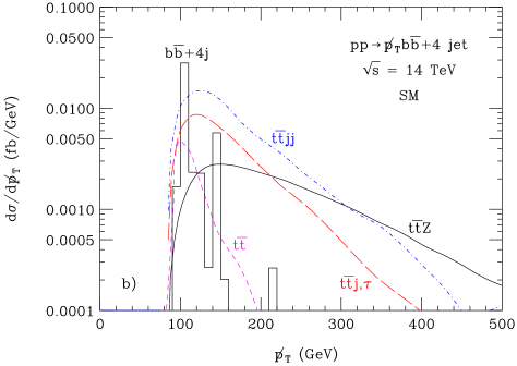
Figure 2: a) The differential cross sections at the LHC as a function of $p_{T}(Z)$ for ${\ell^{\prime}}^{+}{\ell^{\prime}}^{-}\ell\nu b\bar{b}jj$ final states. Shown are the SM predictions for $t\bar{t}Z$ production, for several non-standard $ttZ$ couplings, and for various backgrounds. Only one coupling at a time is allowed to deviate from its SM value. b) The differential cross sections as a function of the missing transverse momentum for $p\hbox to0.0pt{\hss/}_{T}b\bar{b}+4$j production at the LHC. Shown are the SM predictions for $t\bar{t}Z$ production and for various backgrounds.

The $Z$ boson transverse momentum distribution for the trilepton final state is shown in Fig. 2a for the SM signal and backgrounds, as well as for the signal with several non-standard $ttZ$ couplings. Only one coupling at a time is allowed to deviate from its SM prediction. The backgrounds are each more than one order of magnitude smaller than the SM signal. Figure 2a shows that varying $F^{Z}_{1V,A}$ leads mostly to a cross section normalization change, hardly affecting the shape of the $p_{T}(Z)$ distribution. This is because, unlike in the $tt\gamma$ case, there is no radiative top decay, i.e. no $t\bar{t}$ events where $t\to WZb$. This implies that, for the cuts we impose, the $p_{T}(Z)$ distribution for SM couplings and for $F^{Z}_{1V,A}=-F^{Z,SM}_{1V,A}$ are almost degenerate. Currently, the SM $t\bar{t}Z$ cross section is known only at LO, and has substantial factorization and renormalization scale uncertainty. Since the backgrounds are insignificant, this normalization uncertainty, and the sign degeneracy, will ultimately be the limiting factors in extracting anomalous vector and axial vector $ttZ$ couplings.

For the $p\hbox to0.0pt{\hss/}_{T}b\bar{b}+4j$ new final state we require at least 3 jets with $p_{T}>50$ GeV and $p\hbox to0.0pt{\hss/}_{T}>5~{}{\rm GeV}^{1/2}\sqrt{\sum p_{T}}$. The largest backgrounds for this final state come from $t\bar{t}$ and $b\bar{b}+4j$ production where one or several jets are badly mismeasured, from $pp\to t\bar{t}jj$ with $t\bar{t}\to\ell^{\pm}\nu_{\ell}b\bar{b}jj$ and the charged lepton being missed, and from $t\bar{t}j$ production, where one top decays hadronically, $t\to Wb\to bjj$, and the other via $t\to Wb\to\tau\nu_{\tau}b$ with the $\tau$-lepton decaying hadronically, $\tau\to h\nu_{\tau}$.

In Fig. 2b we show the missing transverse momentum distributions of the SM $t\bar{t}Z\to p\hbox to0.0pt{\hss/}_{T}b\bar{b}+4j$ signal (solid curve) and various backgrounds. The most important backgrounds are $t\bar{t}jj$ and $t\bar{t}j$ production. However, the missing transverse momentum distribution from these processes falls considerably faster than that of the signal, and for $p\hbox to0.0pt{\hss/}_{T}>300$ GeV, the SM signal dominates.

V Sensitivity Bounds for $ttV$ Couplings: LHC and ILC

The shape and normalization changes of the photon or $Z$-boson transverse momentum distribution can be used to derive quantitative sensitivity bounds on the anomalous $tt\gamma$ and $ttZ$ couplings. For $t\bar{t}Z$ production, the $\Delta\Phi({\ell^{\prime}}{\ell^{\prime}})$ distribution provides additional information Baur:2004uw . In the following we assume a normalization uncertainty of the SM cross section of $\Delta{\cal N}=30\%$.

Even for a modest integrated luminosity of 30 fb^-1, it will be possible to measure the $tt\gamma$ vector and axial vector couplings, and the dipole form factors, with a precision of typically $20\%$ and $35\%$, respectively. For 300 fb^-1, the limits improve to $4-7\%$ for $F^{\gamma}_{1V,A}$ and to about $20\%$ for $F^{\gamma}_{2V,A}$. At the SLHC, assuming an integrated luminosity of 3000 fb^-1, one can hope to achieve a $2-3\%$ measurement of the vector and axial vector couplings, and a $10\%$ measurement of $F^{\gamma}_{2V,A}$, provided that particle identification efficiencies are not substantially smaller, and the reducible backgrounds not much larger, than what we have assumed.

To extract bounds on the $ttZ$ couplings, we perform a simultaneous fit to the $p_{T}(Z)$ and the $\Delta\Phi({\ell^{\prime}}{\ell^{\prime}})$ distributions for the trilepton and dilepton final states, and to the $p\hbox to0.0pt{\hss/}_{T}$ distribution for the $p\hbox to0.0pt{\hss/}_{T}b\bar{b}+4j$ final state. We calculate sensitivity bounds for 300 fb^-1 and 3000 fb^-1 at the LHC; for 30 fb^-1 the number of events expected is too small to yield meaningful results. For an integrated luminosity of 300 fb^-1, it will be possible to measure the $ttZ$ axial vector coupling with a precision of $15-20\%$, and $F^{Z}_{2V,A}$ with a precision of $50-55\%$. At the SLHC, these bounds can be improved by factors of about 1.6 ($F^{Z}_{2V,A}$) and 3 ($F^{Z}_{1A}$). The bounds which can be achieved for $F^{Z}_{1V}$ are much weaker than those projected for $F^{Z}_{1A}$. As mentioned in Sec. 4, the $p_{T}(Z)$ distributions for the SM and for $F^{Z}_{1V,A}=-F^{Z,SM}_{1V,A}$ are almost degenerate. This is also the case for the $\Delta\Phi({\ell^{\prime}}{\ell^{\prime}})$ distribution. In a fit to these two distributions, therefore, an area centered at $\Delta F^{Z}_{1V,A}=-2F^{Z,SM}_{1V,A}$ remains which cannot be excluded, even at the SLHC. For $F^{Z}_{1V}$, the two regions merge, resulting in rather poor limits. The sensitivity bounds on $\Delta F^{Z}_{1A}$ improve by as much as a factor 2 if $\Delta{\cal N}$ can be reduced from $30\%$ to $10\%$.

Table 1: Sensitivities achievable at $68.3\%$ CL for the anomalous $ttV$ ($V=\gamma,\,Z$) couplings $\widetilde{F}^{V}_{1V,A}$ and $\widetilde{F}^{V}_{2V,A}$ of Eq. (2) at the LHC for integrated luminosities of 300 fb^-1, and the ILC with $\sqrt{s}=500$ GeV (taken from Ref. Abe:2001nq ). Only one coupling at a time is allowed to deviate from its SM value.

coupling	LHC, 300 fb-1	$e^{+}e^{-}$ Abe:2001nq	coupling	LHC, 300 fb-1	$e^{+}e^{-}$ Abe:2001nq
$\Delta\widetilde{F}^{\gamma}_{1V}$	$\matrix{+0.043\\[-4.0pt] -0.041}$	$\matrix{+0.047\\[-4.0pt] -0.047}$ , 200 fb-1	$\Delta\widetilde{F}^{Z}_{1V}$	$\matrix{+0.34\\[-4.0pt] -0.72}$	$\matrix{+0.012\\[-4.0pt] -0.012}$ , 200 fb-1
$\Delta\widetilde{F}^{\gamma}_{1A}$	$\matrix{+0.051\\[-4.0pt] -0.048}$	$\matrix{+0.011\\[-4.0pt] -0.011}$ , 100 fb-1	$\Delta\widetilde{F}^{Z}_{1A}$	$\matrix{+0.079\\[-4.0pt] -0.091}$	$\matrix{+0.013\\[-4.0pt] -0.013}$ , 100 fb-1
$\Delta\widetilde{F}^{\gamma}_{2V}$	$\matrix{+0.038\\[-4.0pt] -0.035}$	$\matrix{+0.038\\[-4.0pt] -0.038}$ , 200 fb-1	$\Delta\widetilde{F}^{Z}_{2V}$	$\matrix{+0.26\\[-4.0pt] -0.34}$	$\matrix{+0.009\\[-4.0pt] -0.009}$ , 200 fb-1
$\Delta\widetilde{F}^{\gamma}_{2A}$	$\matrix{+0.16\\[-4.0pt] -0.17}$	$\matrix{+0.014\\[-4.0pt] -0.014}$ , 100 fb-1	$\Delta\widetilde{F}^{Z}_{2A}$	$\matrix{+0.35\\[-4.0pt] -0.35}$	$\matrix{+0.052\\[-4.0pt] -0.052}$ , 100 fb-1

It is instructive to compare the bounds for anomalous $ttV$ couplings achievable at the LHC with those projected for the ILC. The most complete study of $t\bar{t}$ production at the ILC for general $ttV$ ($V=\gamma,\,Z$) couplings so far is that of Ref. Abe:2001nq . It uses the parameterization of Eq. (2) for the $ttV$ vertex function. In order to compare the bounds of Ref. Abe:2001nq with those anticipated at the LHC, the limits on $F^{V}_{1V,A}$ and $F^{V}_{2V,A}$ have to be converted into bounds on $\widetilde{F}^{V}_{1V,A}$ and $\widetilde{F}^{V}_{2V,A}$. Table 1 compares the bounds we obtain for $\widetilde{F}^{V}_{1V,A}$ and $\widetilde{F}^{V}_{2V,A}$ with those reported for the ILC in Ref. Abe:2001nq . We show LHC limits only for an integrated luminosity of 300 fb^-1. The results of Table 1 demonstrate that the ILC, with the exception of $F^{\gamma}_{1V}$ and $F^{\gamma}_{2V}$, will be able to considerably improve the sensitivity limits which can be achieved at the LHC, in particular for the $ttZ$ couplings.

VI Conclusions

The LHC will be able to perform first tests of the $ttV$ couplings. Already with an integrated luminosity of 30 fb^-1, one can probe the $tt\gamma$ couplings with a precision of about $10-35\%$ per experiment. With higher integrated luminosities one will be able to reach the few percent region. The $t\bar{t}Z$ cross section with leptonic $Z$ decays is roughly a factor 20 smaller than the $t\bar{t}\gamma$ rate. It is therefore not surprising that the sensitivity limits on the $ttZ$ couplings are significantly weaker than those which one expects for the $tt\gamma$ couplings. The ILC, with the exception of $F^{\gamma}_{1V}$ and $F^{\gamma}_{2V}$, will be able to further improve our knowledge of the $ttV$ couplings, in particular in the $ttZ$ case.

This research was supported in part by the National Science Foundation under grant No. PHY-0139953.

References

- (1) F. Abe et al. (CDF Collaboration), Phys. Rev. Lett. 74, 2626 (1995).
- (2) S. Abachi et al. (DØ Collaboration), Phys. Rev. Lett. 74, 2632 (1995).
- (3) D. Chakraborty, J. Konigsberg and D. L. Rainwater, Ann. Rev. Nucl. Part. Sci. 53, 301 (2003).
- (4) F. Larios, M. A. Perez and C. P. Yuan, Phys. Lett. B457, 334 (1999); M. Frigeni and R. Rattazzi, Phys. Lett. B269, 412 (1991).
- (5) T. Abe et al. (American Linear Collider Working Group Collaboration), arXiv:hep-ex/0106057.
- (6) U. Baur, A. Juste, L. H. Orr and D. Rainwater, Phys. Rev. D71, 054013 (2005).
- (7) W. Hollik et al., Nucl. Phys. B551, 3 (1999) [Erratum-ibid. B557, 407 (1999)].
- (8) G. L. Bayatian et al. (CMS Collaboration), CMS Technical Design Report, CERN-LHCC-94-38 (Dec. 1994).
- (9) F. Maltoni and T. Stelzer, JHEP 0302, 027 (2003).
- (10) ATLAS TDR, report CERN/LHCC/99-15 (1999); Ph. Schwemling, ATLAS note SN-ATLAS-2003-034.
- (11) G. Altarelli, L. Conti and V. Lubicz, Phys. Lett. B502, 125 (2001) and references therein.
- (12) M. L. Mangano et al., JHEP 0307, 001 (2003).
- (13) U. Baur, A. Juste, L. H. Orr and D. Rainwater, in preparation.