ANL-HEP-PR-05-48 EFI-05-03 Proton Lifetime and Baryon Number Violating Signatures at the LHC in Gauge Extended Models

Abstract

There exist a number of models in the literature in which the weak interactions are derived from a chiral gauge theory based on a larger group than $SU(2)_{L}\times U(1)_{Y}$. Such theories can be constructed so as to be anomaly-free and consistent with precision electroweak measurements, and may be interpreted as a deconstruction of an extra dimension. They also provide interesting insights into the issues of flavor and dynamical electroweak symmetry breaking, and can help to raise the mass of the Higgs boson in supersymmetric theories. In this work we show that these theories can also give rise to baryon and lepton number violating processes, such as nucleon decay and spectacular multijet events at colliders, via the instanton transitions associated with the extended gauge group. For a particular model based on $SU(2)_{1}\times SU(2)_{2}$, we find that the $B+L$ violating scattering cross sections are too small to be observed at the LHC, but that the lower limit on the lifetime of the proton implies an upper bound on the gauge couplings.

1 Introduction

Baryon ($B$) and lepton ($L$) number seem to be excellent symmetries of Nature, and to date no direct evidence for their violation has been found. Even so, it is very likely that neither of these charges is exactly conserved. For one, the Universe contains many more baryons than anti-baryons, and a necessary ingredient to create such an asymmetry is the violation of baryon number [1]. In addition, the existence of very small neutrino masses may also point toward the violation of lepton number. Such masses can be naturally generated by the see-saw mechanism which typically involves a heavy Majorana neutrino, whose mass violates lepton number by two units [2]. But perhaps the most compelling reason to expect the violation of baryon and lepton number is the fact that these charges are not even conserved by the Standard Model (SM) [3].

In the SM, both $B$ and $L$ are symmetries of the classical Lagrangian, but are violated by quantum corrections. Equivalently, the currents corresponding to these would-be symmetries are anomalous, having non-vanishing divergences. However, the only processes that change the value of these charges in the SM are instanton transitions between degenerate $SU(2)_{L}$ gauge vacua. Each transition violates both $B$ and $L$ by $n_{g}$ units, where $n_{g}$ is the number of generations. The rate for these transitions is proportional to a very small instanton tunnelling factor,

$$\Gamma_{inst}\propto e^{-16\pi^{2}/g_{L}^{2}}\sim e^{-400},$$ (1)

where $g_{L}$ is the $SU(2)_{L}$ gauge coupling. Because of this enormous suppression, $B$ and $L$ violation are effectively non-existent in the SM (at zero temperature) explaining why neither one has been observed. Eq. (1) also indicates that the rate would be much larger if the gauge coupling $g_{L}$ were larger.

Even though the Standard Model provides an excellent description of nearly all particle physics interactions seen so far, there is reason to believe that this model only gives an effective description of Nature below some ultraviolet cutoff scale. Above the cutoff, the SM must be extended to include new physics. In many cases the new physics has additional sources of baryon and lepton number violation. This can occur through new perturbative interactions, such as in grand unified theories and supersymmetric models with $R$-parity violation. The new physics may also violate $B$ and $L$ through non-perturbative phenomena, as in models where the electroweak gauge structure is extended beyond the $SU(2)_{L}\times U(1)_{Y}$ group of the SM. Depending on the fermion charges under this extended gauge group, the instanton transitions in such models can violate $B$ and $L$. Unlike the $SU(2)_{L}$ rate, however, the instanton rates in gauge extended models can be sizeable if the corresponding gauge couplings are reasonably large. This opens the possibility of observable baryon and lepton number violating processes within these models [4].

In the present work, we examine this possibility for a particular gauge extension of the SM. The enlarged electroweak gauge group we consider is $SU(2)_{1}\times SU(2)_{2}\times U(1)_{Y}$. Under this group, the left-handed fermions of the third generation transform as doublets of $SU(2)_{1}$ and singlets of $SU(2)_{2}$, while the left-handed fermions of the first and second generations are doublets of $SU(2)_{2}$ but singlets of $SU(2)_{1}$. The SM electroweak structure is regained by spontaneously breaking $SU(2)_{1}\times SU(2)_{2}$ down to its diagonal $SU(2)$ subgroup, which is identified with the $SU(2)_{L}$ group of the SM. This particular gauge structure arises in several extensions of the SM, such as Topflavor [5], which seeks to motivate the hierarchy in the Yukawa couplings, as well as Non-Commuting Extended Technicolor [6], in which the $SU(2)_{1}$ is associated with the ETC gauge group. Another application arises in supersymmetric theories which increase the tree-level Higgs mass through the $D$-terms of the extra $SU(2)$ [7], as well as supersymmetric models in which baryogenesis is induced by the presence of strongly interacting Higgsinos and gauginos [8]. Finally, this model is expected to capture, through dimensional deconstruction [9], the low energy physics of an extra dimension with $SU(2)$ in the bulk and localized fermions [10].

When $SU(2)_{1}\times SU(2)_{2}$ breaks down to its diagonal subgroup, there are instantonic effects which are not captured by the instantons of the low energy diagonal $SU(2)_{L}$ [11]. Thus, we expect non-perturbative effects in such theories with extended weak interactions to lead to qualitatively new effects. Furthermore, the gauge couplings of the two original $SU(2)$’s must necessarily be stronger than the diagonal coupling $g_{L}$, enhancing the instanton transitions relative to those of $SU(2)_{L}$. In several of the examples above, it is further true that one of the $SU(2)$ gauge couplings is considerably larger than the other. The instanton transitions of this more strongly-coupled subgroup will then be much more frequent than those of the other $SU(2)$. The observable effects of such instantons are two-fold. In the context of particle collider experiments such as the LHC, they can mediate spectacular $B$ and $L$ violating scattering events. On the other hand, the violation of baryon and lepton number also opens the possibility of nucleon decay, and this puts interesting constraints on these models. Even though we are focused on a particular gauge extension of the SM, we also emphasize that we have only made this choice for concreteness. For more general gauge extensions of the SM electroweak sector, we expect that many of our results, as well as the formalism used to obtain them, to carry over in much the same way.

Previous work along these lines has focused on high energy scattering in the SM due to $SU(2)_{L}$ instantons. The results of Refs. [12, 13, 14] suggest that at very high energies, the sum over high-multiplicity exclusive cross sections exponentiates yielding a factor that partially cancels the instanton suppression, and producing a potentially observable inclusive cross section at future colliders such as the VLHC. (See also Refs. [15, 16, 17, 18, 19, 20].) However, the approximations made in these calculations generally break down at energies below which the instanton suppression is significantly reduced. Instead, in the present work we consider only exclusive processes due to the instantons of an extended gauge group. Our results for collider cross sections will therefore represent a conservative lower bound on ($B+L$) violating scattering events in these gauge-extended models at the LHC.

The article is organized as follows. In Section 2 we discuss the structure of the $SU(2)_{1}\times SU(2)_{2}\times U(1)_{Y}$ gauge extension, and describe the bounds on this extension due to precision electroweak measurements. Our main results are contained in Section 3 where we outline the formalism used to describe the instanton transitions within the model, and compute the effective $B+L$ violating operator generated by $SU(2)_{1}$ instantons. In Section 4 we apply this result to calculate the cross section for $B$ and $L$ violating scattering events at the LHC induced by $SU(2)_{1}$ instantons. Section 5 contains an analysis of nucleon decay due to $SU(2)_{1}$ instantons, as well as a discussion of the constraints implied by this possibility. The opposite limit of this scenario, in which the $SU(2)_{2}$ gauge coupling is taken to be large, is considered in Section 6. As in the previous sections, we examine the possibility of nucleon decay and $B+L$ violating scattering. Finally, Section 7 is reserved for our conclusions. Some of the technical details of our calculations are given in the Appendices A, B, and C.

2 A Gauge Extension of the Standard Model

The gauge extension of the Standard Model that we consider in the present work is based on the gauge group $SU(3)_{c}\times SU(2)_{1}\times SU(2)_{2}\times U(1)_{Y}$. The $SU(3)_{c}$ and $U(1)_{Y}$ subgroups coincide identically with those of the SM. On the other hand, the $SU(2)_{L}$ group of the SM is expanded to a larger $SU(2)_{1}\times SU(2)_{2}$ structure. While the gauge structure of the SM is extended in this scenario, the fermion content of the model is identical to the SM. Under the new $SU(2)_{1}$ and $SU(2)_{2}$ groups, the doublets of the third generation transform as doublets under $SU(2)_{1}$ and singlets under $SU(2)_{2}$, while the first and second generation doublets are singlets of $SU(2)_{1}$ and doublets of $SU(2)_{2}$. In other words, their $SU(2)_{1}\times SU(2)_{2}\times U(1)_{Y}$ quantum numbers are

$$Q^{3} = (\mathbf{2},\mathbf{1})_{1/6}$$

$$L^{3} = (\mathbf{2},\mathbf{1})_{-1/2}$$

$$Q^{1,2} = (\mathbf{1},\mathbf{2})_{1/6}$$

$$L^{1,2} = (\mathbf{1},\mathbf{2})_{-1/2}.$$ (2)

The SM gauge structure is regained by giving a vacuum expectation value (VEV) to a bidoublet scalar, $\Sigma$,

$$\Sigma_{i\bar{k}}\to\left<\Sigma_{i\bar{k}}\right>=u\;\delta_{i\bar{k}}.$$ (3)

Under this breaking, the Standard Model $SU(2)_{L}$ group emerges as the unbroken diagonal subgroup of $SU(2)_{1}\times SU(2)_{2}$. The corresponding $SU(2)_{L}$ gauge coupling is

$$g_{L}=\frac{g_{1}g_{2}}{\sqrt{g_{1}^{2}+g_{2}^{2}}}.$$ (4)

This relation implies that when one of the gauge couplings becomes large, the other one approaches $g_{L}$ from above, and thus both $g_{1}$ and $g_{2}$ are necessarily larger than $g_{L}$. The fermion doublets of either $SU(2)_{1}$ or $SU(2)_{2}$ transform as doublets under $SU(2)_{L}$.

At a lower scale, $v\simeq 174$ GeV, the remaining $SU(2)_{L}\times U(1)_{Y}$ electroweak symmetry is broken to $U(1)_{em}$ as in the SM. This is accomplished by giving a VEV to one or more Higgs boson doublets. We will focus on the case of a single $Y=+1/2$ Higgs boson doublet, but our results would be largely unchanged if we included instead a $Y=\pm 1/2$ pair of doublets as in the MSSM. We consider two possible representations for the Higgs boson under $SU(2)_{1}\times SU(2)_{2}$. They are:

$$\Phi = (\mathbf{2},\;\mathbf{1})_{1/2}~{}~{}~{}~{}~{}~{}~{}\Rightarrow\mbox{\emph{heavy} case},$$ (5)

$$\Phi = (\mathbf{1},\;\mathbf{2})_{1/2}~{}~{}~{}~{}~{}~{}~{}\Rightarrow\mbox{\emph{light} case}.$$

In the first case, which we call the heavy case, the Higgs doublet is charged under $SU(2)_{1}$ but not under $SU(2)_{2}$. The opposite is true for the light case. These two possibilities are very similar with regards to instantons, but differ significantly when it comes to the experimental constraints on the model. We will consider them both. In Appendix B we tabulate some important results concerning the gauge bosons, their masses, and their couplings to fermions.

2.1 Precision Electroweak Constraints

The most important experimental constraints on this gauge extended model come from precision electroweak measurements made at LEP, the Tevatron, and the SLC. Due to the enlarged gauge structure, the model has additional heavy gauge bosons, a ${Z^{0}}^{\prime}$ and a ${W^{\pm}}^{\prime}$, and modified relations between the Lagrangian parameters and the electroweak observables. The gauge boson mass matrices and the shifts in the electroweak observables are listed in Appendices B and  C. Because of these changes, the precision electroweak data imposes strong constraints on the model, and on the $SU(2)_{1}\times SU(2)_{2}$ symmetry breaking scale $u$ in particular. The precise constraints are different for the heavy and light cases described above.

The Lagrangian-level parameters of the electroweak sector of the model can be taken to be $\{g_{1},\,g_{2},\,g_{y},\,v,\,u\}$. We find it more convenient to use the equivalent set $\{g_{L},\,v,\,\sin\theta,\,\sin\varphi,\,\delta\}$, where

$$\begin{array}[]{cccccc}g_{L}&=&\frac{g_{1}g_{2}}{\sqrt{g_{1}^{2}+g_{2}^{2}}},&~{}~{}~{}~{}~{}\sin\theta&=&\frac{g_{y}}{\sqrt{g_{y}^{2}+g_{L}^{2}}},\\ \sin\varphi&=&\frac{g_{2}}{\sqrt{g_{1}^{2}+g_{2}^{2}}},&~{}~{}~{}~{}~{}\delta&=&\frac{v^{2}}{2\,u^{2}}.\end{array}$$ (6)

All (tree-level) electroweak observables can be expressed in terms of these. In our analysis, we specify the values of $\delta$ and $\sin\varphi$, and use the measured values of $M_{Z}(M_{Z})$, $\alpha(M_{Z})$, and $G_{F}$ (extracted from the muon decay rate) to fix the rest. We use the values [21],

$$\alpha^{-1}(M_{z}) = 127.918$$

$$G_{F} = 1.16637\times\,10^{-5}\;\mbox{GeV}^{-2}$$

$$M_{Z}(M_{Z}) = 91.1876\;\mbox{GeV}~{}.$$

Having fixed and specified the electroweak parameters, we may calculate the shifts in the electroweak observables due to the extended gauge structure. For example, the shift in the $W$ mass compared to the SM in the light case is

$$M_{W}=(M_{W})_{SM}(1+0.219\,\sin^{4}\varphi\,\delta).$$ (7)

Here, $(M_{W})_{SM}$ should properly be the tree-level expression of the SM. However, if we work to first order in both the loop corrections and the small parameter $\delta$, it is consistent to use the one-loop value of $(M_{W})_{SM}$ in this expression. The shifts in other important electroweak observables are tabulated in Appendix C. A Higgs boson mass of $m_{h}=115$ GeV and a top quark mass of $m_{t}=177$ GeV were used to obtain the SM inputs. For each parameter set we compute the effective reduced $\chi^{2}$:

$$\chi^{2}=\sum_{i=1}^{N}\frac{(\mathcal{O}_{i}-\mathcal{O}_{i}^{exp})^{2}}{\sigma_{i}^{2}},$$ (8)

where $\mathcal{O}_{i}$ is the value of the $i$-th observable in the model, $\mathcal{O}_{i}^{exp}$ is the measured value of this observable, and $\sigma_{i}$ is its experimental uncertainty. We demand that $\chi^{2}/N<1.6$, which corresponds (roughly) to the $95\%~{}c.l.$ exclusion contour for $N=20$ degrees of freedom. (By comparison, the best fit to the SM, for the observables considered, has a $\chi^{2}/N=1.03$.) The exclusion contours are shown in Fig. 1. Observe that in the light case, the bounds on $u$ become very weak for large values of $g_{1}$ because only the third generation sector is affected by the strong interactions (resulting in no large corrections to $G_{F}$ extracted from muon decay), and the mixing between the light and heavy gauge bosons induced by the standard Higgs VEV becomes smaller for larger values of $g_{1}$.

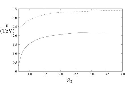
Figure 1: $95\%~{}c.l.$ exclusion contour as a function of $g_{1}$ and $g_{2}$. The allowed region lies above the solid curve  (light case) or the dashed curve (heavy case).

As discussed above, the above bounds on $u$ were obtained for a Higgs mass close to the present experimental bound. These bounds may not be lowered in any significant way by raising the Higgs mass. In the light case, raising the Higgs mass up to values close to 200 GeV produces very small variations in the bound on $u$. In the heavy case, the bound on $u$ increases with the Higgs mass. For instance, for a Higgs boson mass of about 150 GeV, the lower bound on $u$ increases by about 500 GeV for all values of $g_{1}>1.5$.

3 Instanton Induced Operators

In this section, we derive effective operators which describe the instanton-induced interactions at low energies. We begin with some general features of instantons in broken gauge theories, and then specialize to the case of $SU(2)_{1}\times SU(2)_{2}$. It is well-known that non-Abelian gauge theories have many physically distinct vacua separated by energy barriers of finite height. As a result, it is possible for a system prepared in one vacuum state to pass to another by tunnelling. The gauge field configurations that describe this tunnelling are called instantons. As we shall see, if there are fermions charged under the gauge group, each instanton transition is accompanied by the production of fermions. For $SU(2)_{L}$ instantons in the SM, this is the source of $B$ and $L$ violation.

In a pure non-Abelian gauge theory, instanton configurations are solutions of the Euclidean space equations of motion with finite Euclidean action. A given instanton solution is characterized by its spacetime location, $x^{\mu}_{0}$, its Euclidean space radius, $\rho$, and its orientation in the global gauge group space, $U$. The instanton transition amplitude is computed by making a semiclassical expansion of the corresponding functional integral about the instanton solution, working to quadratic order in the fluctuations about this solution. This procedure generates a factor of $e^{-S_{inst}}=e^{-8\pi^{2}/g^{2}}$ from the classical solution, as well as a functional determinant from the fluctuations [3].

The situation becomes more complicated if the gauge theory is spontaneously broken by the expectation value of one or more scalar fields. In this case, exact solutions to the combined gauge/Higgs Euclidean space equations of motion are not known. Nevertheless, it is possible to obtain approximate solutions for a fixed instanton size, $\rho$, as expansions in $\rho\left<\phi\right>$, where $\left<\phi\right>$ is the symmetry breaking VEV [23]. For a given $\rho$, the contribution of the Higgs field to the Euclidean action is [14, 23]

$$S_{Higgs}=2\pi^{2}\rho^{2}\left<\phi\right>^{2}+\mathcal{O}(\lambda\,\rho^{4}\left<\phi\right>^{4}),$$ (9)

where $\lambda$ denotes a quartic coupling for the scalars. The full transition amplitude is given by the fixed–$\rho$ amplitude integrated over instanton size. Since the integrand is proportional to $e^{-S_{Higgs}}$, this integral is cut off at $\rho\left<\phi\right>\sim 1/\sqrt{2\pi^{2}}$ justifying the expansion in this parameter. The leading contribution from the Higgs field to the action, Eq. (9), comes from the kinetic term since interactions are higher order in $\rho\left<\phi\right>$. Thus, if there are several scalar multiplets which develop VEV’s, the leading contribution to the action will be the sum of the individual contributions, each with the form of Eq. (9). Note, however, that it is only possible to neglect the interaction term in $S_{Higgs}$ if the scalar quartic coupling is not too large, $\lambda\ll 2\pi^{2}$, which we will assume in the present work. On the other hand, for $\lambda\to\infty$ the transition amplitude, being proportional to $e^{-S_{Higgs}}$, vanishes [24]. In this limit, the symmetry breaking sector may be represented by a non-linear sigma model, and the vanishing of the transition amplitude can be explained by the existence of a conserved topological current [25]. The transition between the small and large $\lambda$ regimes is an interesting question, but requires a precise specification of the symmetry breaking sector, and is outside the scope of the present work.

If the theory also has fermions that are charged under the gauge group, this picture of vacuum tunnelling is changed in an important way. While the fermions do not modify the classical instanton solution (at lowest order), the functional integral over the quantum fluctuations now includes an integration over the Grassmann-valued fermion fields. The integral vanishes unless it is saturated by fermions from the integrand. For a trivial (zero instanton) background, this leads to a non-zero fermion determinant. However, in an instanton background there exist fermionic fluctuations which do not contribute to the action at quadratic order. These fermion zero modes are nonetheless part of the functional integration, and the amplitude vanishes. In general, for each fermion representation $r$, there are $2\,T(r)$ fermion and no anti-fermion zero modes in a one-instanton background [26].

While the vacuum transition amplitude vanishes if there are fermions coupled to the gauge group, a non-zero result is obtained if an appropriate number of fermion fields, one for each zero mode, are inserted into the functional integral. The instanton transitions are therefore accompanied by the production of fermions. For the case of $SU(2)_{L}$ instantons, there are $4\,n_{g}$ fermion doublets, three quark doublets and one lepton doublet for each generation, and therefore $4\,n_{g}$ zero modes. The corresponding transition violates both $B$ and $L$ by $n_{g}$ units. For $SU(2)_{1}$ and $SU(2)_{2}$ instantons in the gauge-extended model described in the previous section, the result is the same except now $n_{g}=1$ or $2$. Thus, the instantons in all three cases violate $B+L$.

3.1 Instanton Green’s Functions

In this section we describe the calculation of instanton-induced fermion Green’s functions for a general $SU(2)$ gauge theory with $n_{f}$ Weyl fermion doublets, an arbitrary number of fermion singlets, and $n_{s}$ complex scalar doublets. There are $n_{f}$ fermion zero modes in this case, and the resulting Green’s function will involve one of each of the fermion doublets. The presentation here follows the discussions of Ringwald [13] and Espinosa [14]. Both of these, in turn, rely heavily on the results of ’t Hooft [3].

We wish to calculate the Green’s function

$$G(x_{1},\ldots,z_{m})=\left<\prod_{i=1}^{n_{f}}\psi_{i}(x_{i})\;\prod_{j=1}^{n}A_{\mu_{j}}^{a_{j}}(y_{j})\;\prod_{k=1}^{m}H(z_{k})\right>_{1-inst.},$$ (10)

where the $\psi$ are fermions, the $A$ are gauge fields, and the $H$ are (shifted) scalar fields ($\Phi=\left<\phi\right>+H$).

Following [3, 14], the combined gauge boson and Higgs boson instanton solution is

$$A_{\mu} = x_{\nu}\,\Lambda_{\mu\nu}\;\mathscr{A}(x^{2}),$$ (11)

$$\Phi(x) = \phi(x^{2})\;\bar{h},$$

with $\bar{h}=(0,1)^{t}$, and $\Lambda_{\mu\nu}=U\bar{\tau}_{\mu\nu}U^{\dagger}$, where $\bar{\tau}_{\mu\nu}$ is the matrix $\bar{\sigma}_{\mu\nu}$ acting in the $SU(2)$ space and $U$ is an $SU(2)$ matrix describing the instanton orientation. Their explicit forms are listed below and in Appendix A. The functions $\mathscr{A}$ and $\phi$ have asymptotic expressions valid at large and small distances, respectively:

$$\mathscr{A}(x^{2}) = \left\{\begin{array}[]{lr}\frac{1}{g}\,\frac{2\rho^{2}}{x^{2}(x^{2}+\rho^{2})},&x\ll\rho\vspace{0.3cm}\\ \frac{1}{g}\,\rho^{2}M_{W}^{2}\frac{K_{2}(M_{W}x)}{x^{2}},&x\gg\rho\end{array}\vspace{0.3cm}\right.$$ (14)

$$\phi(x^{2}) = \left\{\begin{array}[]{lr}\left(\frac{x^{2}}{x^{2}+\rho^{2}}\right)^{1/2}\left<\phi\right>,&x\ll\rho\vspace{0.3cm}\\ \left<\phi\right>-\frac{1}{2}\rho^{2}m_{h}\left<\phi\right>\frac{K_{1}(m_{h}x)}{x},&x\gg\rho.\end{array}\right.$$ (17)

The long distance forms are leading term expansions in $\rho\langle\phi\rangle$. These functions correspond to the singular gauge, which has the useful property that the gauge fields go to zero at Euclidean infinity.

Using these solutions, the semiclassical approximation to the functional integral gives [14]

$$G(x_{1},\ldots,z_{n}) =$$

$$\phantom{\!\!\!\!\!\!\!\!\!\!\!\!\!\!\!\!\!\!\!\!\!\!\!\!\!\!\!\!\!\!\!\!\!\!\!\!\!\!\!\!\!\!\!\!\!\!}\int\!d^{4}x_{0}\!\int\!d\rho\!\int\!(dU/8\pi^{2})\;\tilde{F}(\rho,\left<\phi\right>;\mu)\;e^{-S_{E}[A_{cl},\Phi_{cl}]}\;\prod_{i=1}^{n_{f}}\psi_{0_{i}}(x_{i}-x_{0})\prod_{j=1}^{n}A_{cl}(y_{j}-x_{0})\prod_{k=1}^{m}H_{cl}(z_{k}-x_{0}),$$

where $A_{cl}$ and $\Phi_{cl}$ are the classical instanton solutions given above ($H_{cl}=\Phi_{cl}-\left<\phi\right>$), and $\psi_{0_{i}}$ is the $i$-th fermion zero mode in the instanton background. The integrals over the instanton size $\rho$, location $x_{0}$, and group orientation $U$ correspond to collective coordinates for the functional integrations over the zero modes of the gauge field fluctuations. Finally, $\tilde{F}(\rho,\left<\phi\right>;\mu)$ is a product of functional determinants for the non-zero vector, scalar, and fermion modes, along with the Jacobian factors from converting to collective coordinates.

For the approximate instanton solution in the combined gauge/Higgs system, the Euclidean action at leading order in $\rho\left<\phi\right>$ is given by

$$S_{E}[A_{cl},\Phi_{cl}]=\frac{8\pi^{2}}{g(\mu)^{2}}+2\pi^{2}\rho^{2}\,\mathcal{V}^{2}$$ (19)

where

$$\mathcal{V}^{2}=\sum_{k=1}^{n_{s}}\left<\phi_{k}\right>^{2}.$$ (20)

The factors comprising $\tilde{F}(\rho,\left<\phi\right>;\mu)$ were calculated in [3],

$$\tilde{F}(\rho,\left<\phi\right>;\mu)=C\,g^{-8}(\rho\mu)^{b_{0}}\rho^{n_{f}/2-5}$$ (21)

where

$$b_{0}=\frac{22}{3}-\frac{1}{3}\,n_{f}-\frac{1}{6}\,n_{s}$$ (22)

is the one loop beta-function coefficient, and the constant $C$ is given by

$$C=2^{10}\pi^{6}\,\exp\left[\left(8-\frac{1}{2}n_{f}\right)\,\xi_{a}-\left(\frac{2}{3}-\frac{1}{6}n_{f}+\frac{1}{6}n_{s}\right)\xi_{b}-\alpha(1)+(n_{f}-n_{s})\alpha\left(\frac{1}{2}\right)\right].$$ (23)

Here, $(\xi_{a},\xi_{b})=(0,-5/12)$ for $g(\mu)$ defined in the $\overline{MS}$ scheme, and $\alpha(1)$ and $\alpha(1/2)$ are numerical constants with the approximate values

$$\alpha(1)\simeq 0.443,\phantom{AAAAAAA}\alpha(1/2)\simeq 0.146.$$ (24)

The additional factors of $\rho$ are inserted to get the dimensions right. Note also that the combination $\mu^{b_{0}}e^{-8\pi^{2}/g(\mu)^{2}}$ is RG-invariant at one-loop order.

Upon Fourier transforming, the $d^{4}x_{0}$ integral generates a total momentum conserving delta function. The momentum space Green’s function, cancelling off a $(2\pi)^{4}\,\delta^{(4)}(\sum p_{i})$ factor, is therefore

$$\tilde{G}(\{p\},\{q\},\{k\})=\int\!(dU/8\pi^{2})\!\int\!d\rho\;\tilde{F}(\rho,\left<\phi\right>;\mu)\;e^{-S_{E}[A_{cl},\Phi_{cl}]}\;\prod_{i=1}^{n_{f}}\tilde{\psi}_{0_{i}}(p_{i})\prod_{j=1}^{n}\tilde{A}_{cl}(q_{j})\prod_{k=1}^{m}\tilde{H}_{cl}(k_{k}),$$ (25)

where $\tilde{\psi}_{0}$, $\tilde{H}_{cl}$, and $\tilde{A}_{cl}$ denote the Fourier transforms.

3.2 Fermion Zero Modes

To proceed, we need explicit expressions for the fermion zero modes, and for this, we must specify the couplings between the fermions and the scalars. We will focus on the gauge extended model described in Section 2, and look at the instantons of the $SU(2)_{1}$ group that couples to the third generation and the Higgs doublet (heavy case). These solutions are identical to those for $SU(2)_{L}$ instantons obtained in Ref. [14], and also carry over directly for $SU(2)_{2}$ instantons in the light case. Unlike Ref. [14], however, we use a slightly different set of Euclidean space spinor conventions, and because of this, our results are somewhat different in appearance. These conventions are listed in Appendix A.

In Euclidean space, unlike Minkowski space, the two spinor representations of $SO(4)$ are not related by complex conjugation. Instead, the two $SO(4)$ representations, which we label by $A$ and $B$, are related to those of $SO(1,3)$ via the correspondence

$$\begin{array}[]{cccccc}\psi_{R}&\leftrightarrow&\psi_{A},\phantom{AAA}&\psi_{L}&\leftrightarrow&\psi_{B},\\ \psi_{R}^{\dagger}&\leftrightarrow&\psi_{B}^{\dagger},\phantom{AAA}&\psi_{L}^{\dagger}&\leftrightarrow&\psi_{A}^{\dagger}.\end{array}$$ (26)

Using this relation, the equations satisfied by the quark zero modes are

$$0 = \bar{\sigma}_{\mu}{D}_{\mu}\,Q_{B},-i\lambda_{u}\epsilon\,\Phi^{*}_{cl}\,u_{A}-i\lambda_{d}\,\Phi_{cl}\,d_{A},$$

$$0 = \sigma_{\mu}{\partial}_{\mu}u_{A}-i\lambda_{u}\,\Phi^{t}_{cl}\epsilon\,Q_{B},$$ (27)

$$0 = \sigma_{\mu}{\partial}_{\mu}d_{A}+i\lambda_{d}\,\Phi^{\dagger}_{cl}\,Q_{B},$$

where $D_{\mu}={\partial}_{\mu}-igA_{cl\,\mu}$, $\epsilon=i\sigma^{2}$, and the $\lambda_{i}$ are Yukawa interactions. $Q_{B}$ corresponds to the left-handed quark doublet, $u_{A}$ and $d_{A}$ are the Euclidean forms of the right-handed singlets, and $\Phi_{cl}$ and $A_{cl}$ denote the classical instanton solutions given above. The equations for the lepton zero modes have the same form.

To solve Eqs. (3.2), we insert the background solutions from Eqs. (11) and (14), and use the ansatz

$$\psi_{B}=x_{\mu}\sigma_{\mu}\,\varphi(x^{2}),\phantom{AAA}\psi_{A}=\psi_{A}(x^{2}),$$ (28)

where $\varphi(x^{2})$, like $\psi$, denotes a two-component fermion. The long-distance equations can be simplified by making use of $\mathscr{A}(x^{2})\to 0$ and $\phi(x^{2})\to\left<\phi\right>$ for $|x^{2}|\gg\rho^{2}$. The solutions in this case are

$$\psi_{B} = \frac{1}{2\pi}\rho\,m^{2}\frac{K_{2}(m\,x)}{x^{2}}x_{\mu}\sigma_{\mu}\;U^{\dagger}\chi,$$

$$\psi_{A} = \frac{1}{2\pi}\rho\,m^{2}\frac{K_{1}(m\,x)}{x}\,U^{\dagger}\chi,$$ (29)

where $m$ is the fermion mass, and $\chi$ represents a two-component spinor equal to $\chi={-1\choose\>0}$ for $\psi=d$ and $\chi={0\choose 1}$ for $\psi=u$. At short distances, $|x^{2}|\ll\rho^{2}$, the solutions at leading order in $\rho\left<\phi\right>$ are given by

$$\psi_{B} = \frac{1}{\pi}\frac{\rho}{(x^{2})^{1/2}(x^{2}+\rho^{2})^{3/2}}x_{\mu}\sigma_{\mu}\;U^{\dagger}\chi$$

$$\psi_{A} = \frac{i}{2\pi}\rho\,m\frac{1}{x^{2}+\rho^{2}}\,U^{\dagger}\chi.$$ (30)

To obtain the low-energy effective operators generated by the instanton, we will need the Fourier transforms of the long distance zero-mode solutions given by Eq. (3.2). The following (Euclidean space) identities are useful for this:

$$\int d^{4}x\;e^{-ip\cdot x}f(x^{2}) = \frac{4\pi^{2}}{p}\int_{0}^{\infty}dr\;J_{1}(pr)\,r^{2}\,f(r^{2}),$$

$$\int d^{4}x\;e^{-ip\cdot x}\,x_{\mu}\,f(x^{2}) = -{4\pi^{2}\,i}\,\frac{p_{\mu}}{p^{2}}\int_{0}^{\infty}dr\;J_{2}(pr)\,r^{3}\,f(r^{2}),$$ (31)

and

$$\int_{0}^{\infty}dr\;J_{2}(pr)\,r\,K_{n}(m\,r)=\frac{p^{n}}{m^{n}(p^{2}+m^{2})},$$ (32)

where $p=(|p_{\mu}p_{\mu}|)^{1/2}$. Applying these identities to the previous result, we find

$$\tilde{\psi}_{B}(p) = -2\pi\,i\,\rho\left(\frac{p_{\mu}\sigma_{\mu}}{p^{2}+m^{2}}\right)\,U^{\dagger}\chi,$$ (33)

$$\tilde{\psi}_{A}(p) = -2\pi\,i\,\rho\left(\frac{m}{p^{2}+m^{2}}\right)\,U^{\dagger}\chi.$$

In the above, the tildes denote Fourier transformed functions. Since the fermions are massive, it helps to assemble them into a Dirac fermion and revert to Minkowski space. The result is

$$\tilde{\Psi}(p) = 2\pi\,i\,\frac{\rho}{p^{2}-m^{2}}\left(p_{\mu}\gamma^{\mu}\,P_{R}+m\,P_{R}\right){U^{\dagger}\chi\choose U^{\dagger}\chi}$$

$$= \frac{i(p_{\mu}\gamma^{\mu}+m)}{p^{2}-m^{2}}\left[2\pi\rho{0\choose U^{\dagger}\chi}\right].$$

As before, $\chi={-1\choose\>0}$ for $\Psi=d,\;e$, and $\chi={0\choose 1}$ for $\Psi=u,\,\nu$.

The same Bessel function and Fourier transform identities can be applied to obtain the long distance forms of the classical gauge and Higgs boson solutions given in Eqs. (11), (14). Reverting to Minkowski space, they are [14]

$$\tilde{A}_{cl_{\mu}}(p) = \frac{i}{g}\;\frac{4\pi^{2}\,\rho^{2}}{p^{2}-m_{A}^{2}}\,U\bar{\tau}_{\mu\nu}U^{\dagger}p_{\nu},\vspace{0.2cm}$$

$$\tilde{H}_{cl}(p) = -\frac{2\pi^{2}\rho^{2}\left<\phi\right>}{p^{2}-m_{H}^{2}}.$$ (35)

3.3 Instanton Amplitudes

With the explicit zero-mode expressions in hand, we may now construct amplitudes for instanton-induced processes. Applying the LSZ procedure [27] to Eq. (25), and using Eqs. (3.2) and (35), the one-instanton amplitude for a process involving $n_{g}$ SM generations ($n_{f}=4\,n_{g}$), $n$ gauge bosons, and $m$ scalars is given by [14]

$$\mathcal{A} = \frac{C}{g^{8+n}}\mu^{b_{0}}e^{-8\pi^{2}/g^{2}(\mu)}(4\pi^{2})^{n}(2\pi^{2})^{m}(2\pi)^{4n_{g}}V^{m}\cdot$$ (36)

$$\phantom{AAA}\cdot\left(\int_{0}^{\infty}d\rho\;\rho^{6n_{g}-5+2m+2n+b_{0}}e^{-2\pi^{2}\mathcal{V}^{2}\rho^{2}}\right)\;\int({dU}/{8\pi^{2}})\;h(U),$$

where

$$h(U)=\prod_{i=1}^{4n_{g}}\bar{\eta}_{i}(p){0\choose U^{\dagger}\chi}\prod_{j=1}^{n}\epsilon_{\mu}^{(j)}(q_{j})q_{j\nu}tr(U\bar{\tau}_{\mu\nu}U^{\dagger}\mathscr{P}_{j}),$$ (37)

where $\eta_{i}(p)=u_{i}(p)$ or $v_{i}(p)$ is the external state polarization spinor, and $\mathscr{P}$ projects onto the appropriate gauge boson mass eigenstate.

The $\rho$ integral is straightforward, and gives the factor

$$\frac{1}{2}\left(\frac{1}{2\pi^{2}\mathcal{V}^{2}}\right)^{3n_{g}-2+m+n+b_{0}/2}\Gamma(3n_{g}-2+m+n+b_{0}/2).$$ (38)

The resulting amplitude (up to an overall phase) is therefore

$$\mathcal{A} = \frac{C}{g^{8+n}}e^{-8\pi^{2}/g^{2}(\mu)}\left(\frac{1}{4\pi^{2}}\right)^{n_{g}-2+b_{0}/2}\,2^{3n_{g}-3+n+b_{0}/2}\,\Gamma(3n_{g}-2+m+n+b_{0}/2)\,\left(\frac{\mu}{\mathcal{V}}\right)^{b_{0}}\cdot$$ (39)

$$\phantom{AAAAA}\cdot\left(\frac{1}{\mathcal{V}^{2}}\right)^{3n_{g}-2+m/2+n}\;\int({dU}/{8\pi^{2}})\;h(U).$$

In these expressions $\mathcal{V}^{2}$ is the orthogonal sum of the scalar VEV’s, Eq. (20). For the case of $SU(2)_{1}$ or $SU(2)_{2}$ instantons, the bidoublet field $\Sigma$ transforms as a pair of doublets under of these groups, each of which develops a VEV equal to $u\sim\mbox{TeV}$. Thus

$$\mathcal{V}^{2}=v^{2}+2\,u^{2}\simeq 2\,u^{2}\phantom{AAAAA}SU(2)_{1}~{}\mbox{or}~{}SU(2)_{2}~{}\mbox{instantons}.$$ (40)

The VEV of the $\Sigma$ field is along a singlet component of $SU(2)_{L}$, and therefore

$$\mathcal{V}^{2}=v^{2}\phantom{AAAAA}SU(2)_{L}~{}\mbox{instantons}.$$ (41)

3.4 Instanton Effective Operators for $SU(2)_{1}$

For the remainder of this section, we will focus on the situation in which $g_{1}\gg g_{2}$, where the instantons of the $SU(2)_{1}$ gauge theory become unsupressed. We would like to represent the amplitude for these instantons, Eq. (39), by an effective operator valid below the $SU(2)_{1}$-breaking scale. The amplitude found above corresponds to the Green’s function $\left<q^{1}(p_{1})\,q^{2}(p_{2})\,q^{3}(p_{3})\,l(p_{4})\right>$, and consists of one zero mode wavefunction for each fermion, a numerical prefactor, integrations over the instanton size $\rho$ and orientation $U$, and an overall factor of $(2\pi)^{4}\delta^{(4)}(p_{1}+p_{2}+p_{3}+p_{4})$ from the integration over instanton location. Since only the total momentum is conserved, we will be able to represent the large-distance instanton effects by a local operator. Note that since we will use the long-distance expressions of the fermion zero modes, which lose validity at energy scales of order $E_{u}\simeq\sqrt{2}\pi u$, the derived effective theory will also lose validity at energies larger than $E_{u}$.

For the task at hand, it is more convenient to look at the operator generated by an anti-instanton. In this case, the non-vanishing Green’s function is $\left<\bar{q}^{1}\bar{q}^{2}\bar{q}^{3}\bar{l}\right>$. After applying the LSZ procedure, each of the four fermion zero modes generates a factor of the form

$$2\pi\,\rho\left(\chi^{\dagger}U,\;0\right)\eta(p),$$ (42)

where $\eta(p)=u(p)$ or $v(p)$ is the external-state polarization spinor. The resulting amplitude is therefore proportional to

$$(2\pi\,\rho)^{4}\,\int dU\,\left(\chi_{1}^{\dagger}U,\;0\right)\eta_{1}(p_{1})\cdot\left(\chi_{2}^{\dagger}U,\;0\right)\eta_{2}(p_{2})\cdot\left(\chi_{3}^{\dagger}U,\;0\right)\eta_{3}(p_{3})\cdot\left(\chi_{4}^{\dagger}U,\;0\right)\eta_{4}(p_{4}),$$ (43)

with $\chi_{i}={0\choose 1}$ for $u$ or $\nu$, and $\chi_{i}={-1\choose 0}$ for $d$ or $e$.

To perform the integration over instanton orientation $U$, we make use of the fact that, as a manifold, $SU(2)$ is equivalent to $S^{3}$. This equivalence allows us to parametrize an arbitrary $SU(2)$ element as

$$U = e^{i\,\alpha\,\hat{n}\cdot\vec{\sigma}}$$ (44)

$$= \cos(\alpha)+i\,(\hat{n}\cdot\sigma)\sin(\alpha),$$

$$= \left(\begin{array}[]{cc}\cos\alpha+i\sin\alpha\,\cos\theta&i\,e^{-i\phi}\,\sin\alpha\,\sin\theta\\ i\,e^{i\phi}\,\sin\alpha\,\sin\theta&\cos\alpha-i\sin\alpha\,\cos\theta\end{array}\right)$$ (47)

where $\hat{n}=(\sin\theta\cos\phi,\sin\theta\sin\phi,\cos\theta)$ is a unit 3-vector.

The coordinate ranges are

$$\alpha\in[0,\,\pi],\phantom{AAA}\theta\in[0,\,\pi],\phantom{AAA}\phi\in[0,\,2\pi],$$ (48)

and the integration measure is

$$\int\,dU=\int_{0}^{\pi}\!d\alpha\sin^{2}\alpha\int_{-1}^{1}\!d(\cos\theta)\int_{0}^{2\pi}\!d\phi.$$ (49)

The Green’s functions $\left<\bar{q}^{1}\bar{q}^{2}\bar{q}^{3}\bar{l}\right>$ all contain the product of four $U$ matrix elements: each up-type fermion (quark or lepton) gives a factor of $\chi_{u}^{\dagger}U\,u_{L}=(U_{21},U_{22})u_{L}$; each down-type fermion produces a factor $\chi_{d}^{\dagger}U\,d_{L}=(-U_{11},-U_{12})d_{L}$. The resulting integrals are straightforward, and most of them vanish. The only non-zero combinations are

$$U_{11}^{2}U_{22}^{2} \to 2\pi^{2}/3,$$

$$(U_{12}U_{21})^{2} \to 2\pi^{2}/3,$$ (50)

$$U_{11}U_{22}U_{12}U_{21} \to -\pi^{2}/3.$$

Because of this, the only non-zero Green’s functions are

$$\bar{u}\bar{u}\bar{d}\bar{e},\phantom{AAA}\mbox{and}\phantom{AAA}\bar{u}\bar{d}\bar{d}\bar{\nu},$$ (51)

and therefore conserve $U(1)_{em}$. Adding $SU(3)_{c}$ indices, there are six independent Green functions:

$$\begin{array}[]{cc}\bar{u}^{1}\bar{u}^{2}\bar{d}^{3}\bar{e},&\>\>\>\>\bar{u}^{1}\bar{d}^{2}\bar{d}^{3}\bar{\nu},\\ \bar{u}^{1}\bar{d}^{2}\bar{u}^{3}\bar{e},&\>\>\>\>\bar{d}^{1}\bar{u}^{2}\bar{d}^{3}\bar{\nu},\\ \bar{d}^{1}\bar{u}^{2}\bar{u}^{3}\bar{e},&\>\>\>\>\bar{d}^{1}\bar{d}^{2}\bar{u}^{3}\bar{\nu}.\\ \end{array}$$ (52)

These all come in with the same sign because of the ordering of the zero mode integrations in the functional integral. They all have the same numerical prefactor, as well.

Consider now the Green’s function for $\bar{u}^{1}\bar{u}^{2}\bar{d}^{3}\bar{e}$. The corresponding amplitude is proportional to

$$\int dU\;(U_{21},U_{22})u_{L}^{1}\;(U_{21},U_{22})u_{L}^{2}\;(U_{11},U_{12})d_{L}^{3}\;(U_{11},U_{12})e_{L}$$

$$= \frac{2\pi^{2}}{3}\left[u_{L_{1}}^{1}u_{L_{1}}^{2}d_{L_{2}}^{3}e_{L_{2}}+u_{L_{2}}^{1}u_{L_{2}}^{2}d_{L_{1}}^{3}e_{L_{1}}-\frac{1}{2}(u_{L_{1}}^{1}u_{L_{2}}^{2}+u_{L_{2}}^{1}u_{L_{1}}^{2})(d_{L_{1}}^{3}e_{L_{2}}+d_{L_{2}}^{3}e_{L_{1}})\right],$$

where $u_{L},d_{L},e_{L}$ denote the external polarization vectors, and the lower indices are spinorial. This amplitude can be reproduced at lowest order by adding to the low-energy effective Lagrangian the operator

$$\left[u_{L_{1}}^{1}u_{L_{1}}^{2}d_{L_{2}}^{3}e_{L_{2}}+u_{L_{2}}^{1}u_{L_{2}}^{2}d_{L_{1}}^{3}e_{L_{1}}-\frac{1}{2}(u_{L_{1}}^{1}u_{L_{2}}^{2}+u_{L_{2}}^{1}u_{L_{1}}^{2})(d_{L_{1}}^{3}e_{L_{2}}+d_{L_{2}}^{3}e_{L_{1}})\right],$$ (54)

$$= \frac{1}{2}(u_{L}^{1}\cdot e_{L})(u_{L}^{2}\cdot d_{L}^{3})-\frac{1}{2}(u_{L}^{1}\cdot d_{L}^{3})(u_{L}^{2}\cdot e_{L}),$$

where now the $u_{L},d_{L}$ and $e_{L}$ represent the field operators, and in the last line we have re-expressed the operator in a manifestly Lorentz-invariant form.

It should also be possible to connect up the color indices with an $\epsilon^{abc}$ tensor since the effective operator is expected to be invariant under $SU(3)_{c}$. Notice that

$$\epsilon^{abc}u^{a}u^{b}d^{c}=2(u^{1}u^{2}d^{3}+u^{1}d^{2}u^{3}+d^{1}u^{2}u^{3}).$$ (55)

Therefore, we can combine all the $uude$ operators into

$$\frac{1}{2}\epsilon^{abc}\frac{1}{2}\left[(u_{L}^{a}\cdot e_{L})(u_{L}^{b}\cdot d_{L}^{c})-(u_{L}^{a}\cdot d_{L}^{c})(u^{b}_{L}\cdot e_{L})\right]$$ (56)

$$= \frac{1}{2}\epsilon^{abc}\;(u_{L}^{a}\cdot e_{L})(u^{b}_{L}\cdot d^{c}_{L}).$$

Exactly the same thing can be done for the $udd\nu$ operators.

Putting everything together, the effective four-fermion operator corresponding to a single $SU(2)_{1}$ anti-instanton is

$$\mathcal{O}_{\rm{eff}} = \frac{C}{g_{1}^{8}}\,e^{-8\pi^{2}/g_{1}^{2}(\mu)}\left(\frac{1}{4\pi^{2}}\right)^{b_{0}/2-1}2^{b_{0}/2}\left(\frac{\mu}{{\mathcal{V}}}\right)^{b_{0}}\,\Gamma(1+b_{0}/2)\,\left(\frac{\pi^{2}}{3V_{g}}\right)\cdot$$ (57)

$$\phantom{AAAAAAAAA}\cdot\left(\frac{1}{{\mathcal{V}}^{2}}\right)\,\epsilon^{abc}\,\left[(u_{L}^{a}\cdot e_{L})(u^{b}_{L}\cdot d^{c}_{L})+(d_{L}^{a}\cdot\nu_{L})(d^{b}_{L}\cdot u_{L}^{c})\right].\phantom{{A\choose A}}$$

where $V_{g}=8\pi^{2}$ is four times the group volume, $b_{0}$ is the one-loop beta-function coefficient, ${\mathcal{V}}\simeq\sqrt{2}\,u$, and the constant $C$ is given in Eq. (23). This operator is also invariant under $SU(2)_{L}$, and violates both $B$ and $L$ by one unit each.

4 $B+L$-Violating Scattering by $SU(2)_{1}$ Instantons

As a first application of the results of Section 3, we compute the scattering cross section for $bb\to\bar{t}\bar{\nu}$ due to $SU(2)_{1}$ instantons. We will focus on this particular process because of all the $B+L$ violating reactions induced by the operator in Eq. (57), this one is expected to have the largest cross section at the LHC. To see why, note that this operator involves only third generation fermions. As a result, when the parton-level cross section is convolved with parton distribution functions (PDF’s) to obtain the total hadronic cross section, it will be suppressed by the small PDF’s of the third-generation fermions within the proton. This suppression is fairly strong for the bottom quark, but extremely strong for the top quark. Therefore, events with only bottom quarks in the initial state are expected to produce the largest cross sections.

The parton level cross section is computed straightforwardly using the operator from Eq. (57). Inserting the $\epsilon^{abc}(b_{L}^{a}\cdot\nu_{L})(b_{L}^{b}\cdot t^{c}_{L})$ operator in the corresponding matrix element, and squaring, summing, and averaging over spins and colors, we find

$$\epsilon^{abc}(b_{L}^{a}\!\cdot\!\nu_{L})(b_{L}^{b}\!\cdot\!t^{c}_{L})\to\frac{2}{3}\left[2(p_{1}\!\cdot\!p_{3})(p_{2}\!\cdot\!p_{4})+2(p_{1}\!\cdot\!p_{4})(p_{2}\!\cdot\!p_{3})-(p_{1}\!\cdot\!p_{2})(p_{3}\!\cdot\!p_{4})\right],$$ (58)

where $p_{1}$ and $p_{2}$ are the incoming momenta, and $p_{3}$ and $p_{4}$ are the outgoing momenta. The parton-level cross section then follows in the usual way. To get the total cross section in a $pp$ hadron collider such as the LHC, we must convolve this cross section with the bottom quark PDF’s of the proton. Thus

$$\sigma_{tot}=\int_{0}^{1}dx_{1}\int_{0}^{1}dx_{2}\;f_{{b}}(x_{1})f_{{b}}(x_{2})\;\sigma(s=x_{1}x_{2}\,s_{0}),$$ (59)

where $\sqrt{s_{0}}$ is the $pp$ center-of-mass (CM) energy. Since the bottom quark PDF’s peak at small $x$, a large CM energy is needed to avoid a strong additional suppression of the total cross section.

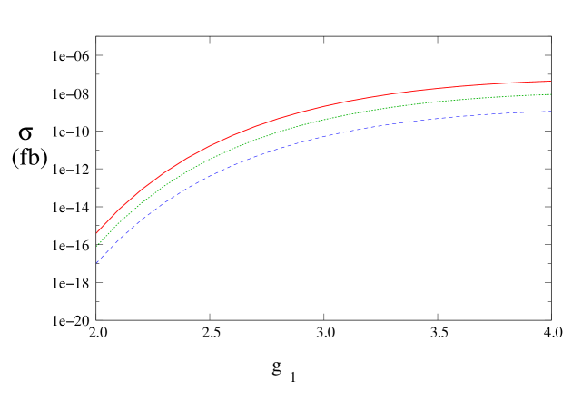
Figure 2: The $SU(2)_{1}$ instanton mediated ${b}{b}\to\bar{t}\bar{\nu}_{\tau}$ cross section at $\sqrt{s_{0}}=14$ TeV for $u=2$ TeV (solid red), $u=3$ TeV (dotted green), and $u=5$ TeV (dashed blue).

Fig. 2 shows the cross section for $bb\to\bar{t}\bar{\nu}_{\tau}$ scattering at the LHC, with $\sqrt{s_{0}}=14$ TeV. The three lines in this figure correspond to three different values of the $SU(2)_{1}\times SU(2)_{2}$ symmetry breaking VEV: $u=2$ TeV, 3 TeV, and 5 TeV. The CTEQ6M parton distributions from Ref. [28] were used to evaluate Eq. (2). Unfortunately, this $B+L$ violating cross section is unobservably small at the LHC, even for larger values of the gauge coupling. The reason why may be understood by examining the various factors that contribute to the instanton amplitude of Eq. (39). For $g_{1}\simeq 3$, the usual instanton term, $e^{-8\pi^{2}/g_{1}^{2}}$, is still fairly small, and there is an additional suppression by the $1/g_{1}^{8}$ term in the amplitude. Together, they contribute a factor of order $10^{-8}$. This is offset somewhat by the large prefactor $C$, given in Eq. (23), which is of order $10^{5}$ in the present case, but not enough for the cross section to be observable. We would also like to emphasize that for very large values of the gauge coupling $g_{1}$, the semi-classical approximation used to derive the effective instanton operator is expected to break down.

5 Proton Decay from $SU(2)_{1}$ Instantons

The observed stability of the proton often leads to very strong constraints on theories beyond the Standard Model which contain baryon number violating interactions. This is true for the $SU(2)_{1}\times SU(2)_{2}$ extension considered here since the operator of Eq. (57) violates $B$ and $L$ by one unit, and can induce the decay of the proton into a meson and a light lepton. As we shall see below, the experimental limit on the proton lifetime implies a lower bound on the $SU(2)_{1}$-breaking scale $u$, and an upper bound on the gauge coupling $g_{1}$.

For $SU(2)_{1}$ instanton induced decays to occur, however, the third generation quarks must be connected with the first generation quarks that make up the proton. Such a link is provided by the flavor-changing couplings of the quarks with the W gauge bosons. The Feynman diagrams for the process $p\to K^{+}\bar{\nu}_{\tau}$ generated in this way are shown in Fig. 3. Both of these are suppressed by two loop factors. A second possibility, that avoids this loop suppression, is that the light quark mass eigenstates in the proton contain a small admixture of the third generation gauge eigenstates that couple directly to $SU(2)_{1}$. This generates a contribution to the proton decay amplitude that is not suppressed by any loop factors, but does involve elements of the up and down quark mixing matrices. Since these elements are unknown (only their product is measured through the CKM matrix), we will ignore this possibility and focus solely on the contributions involving $W$ boson loops. Barring unusual cancellations, this will set a lower bound on the instanton-induced proton decay rate.

aa

Figure 3: Feynman diagrams for anti-instanton mediated proton decay.

The operator responsible for $p\to K^{+}\bar{\nu}_{\tau}$ decay is the $\epsilon^{abc}(t_{L}^{a}\!\cdot\!b_{L}^{b})(b_{L}^{c}\!\cdot\!\tau_{L})$ term in Eq. (57). By connecting the legs of this operator to first and second generation quarks through $W$ bosons, as shown in Fig. 3, we obtain a pair of operators that directly mediate proton decay. Both of these diagrams involve a pair of loop integrations, and in each case the two loops are independent as a result of the locality of the effective operator.

The loop integrals all have the form

$$I_{\mu\nu}=\int\frac{d^{4}k}{(2\pi)^{4}}\frac{(p_{a}-k)_{\mu}}{[(p_{a}-k)^{2}-m_{a}^{2}]}\frac{(p_{b}-k)_{\nu}}{[(p_{b}-k)^{2}-m_{b}^{2}]}\frac{1}{k^{2}-M_{W}^{2}},$$ (60)

where $p_{a}$ and $p_{b}$ are the external momenta, and $m_{a}$ and $m_{b}$ are the fermion masses in the loop. This integral is logarithmically divergent in the ultraviolet. The reason for this apparent divergence is that we have used the long-distance form of the fermion zero modes, which go as $p_{\mu}/p^{2}$, as shown in Eq. (3.2). For scales above $\rho^{-1}$, however, this form is no longer valid, and should be replaced by the Fourier transform of the short-distance form for the zero modes. From Eq. (3.2), we find that these go as

$$x_{\mu}f(r)=\frac{x_{\mu}}{r(r^{2}+\rho^{2})^{3/2}},$$ (61)

where $r=(|x^{2}|)^{1/2}$. The Fourier transform can be computed using the identity

$$\int d^{4}xe^{ip\cdot x}x_{\mu}f(r)=4\pi^{2}\,i\frac{p_{\mu}}{p^{2}}\int_{0}^{\infty}drJ_{2}(pr)r^{3}f(r).$$ (62)

For large $p$, $J_{2}(pr)\simeq\sqrt{\frac{2}{\pi\,pr}}\,\cos(pr-5\pi/4)$. The resulting $r$ integral is finite, and the momentum-space wavefunction falls off at least as fast as $p^{-3/2}$ for large $p$. Using this form in the loop integration at large momenta, the full integral is found to be convergent. Taking this fact into account, we will approximate the result of the loop integrals, Eq. (60), by cutting them off at a scale $\Lambda\sim\rho^{-1}\sim\sqrt{2}\pi\,u$, where our effective operator description is expected to break down.

Setting the external momenta $p_{a}$ and $p_{b}$ to zero in Eq. (60) and performing the integration, we find

$$I_{\alpha\beta}=\eta_{\alpha\beta}\;\frac{i}{8(2\pi)^{2}}\int_{0}^{1}\!dx\,dy\,dz\,\delta(1-x-y-z)\,\left[\ln\left(1+\frac{\Lambda^{2}}{\Delta}\right)-\frac{3}{2}\right]+\mathcal{O}\left(\frac{\Delta}{\Lambda^{2}}\right),$$ (63)

with $\Delta$ given by

$$\Delta=x\,m_{a}^{2}+y\,m_{b}^{2}+z\,M_{W}^{2}+\mathcal{O}(p_{1}^{2},p_{2}^{2}).$$ (64)

The integrals over $x$, $y$, and $z$ can be done analytically, and the result is

$$I_{\alpha\beta} = \eta_{\alpha\beta}\,A(m_{a}^{2},m_{b}^{2},M_{W}^{2})$$

$$= \eta_{\alpha\beta}\;\frac{i}{16(2\pi)^{2}}\left[-\frac{1}{2}+f_{\Lambda}(m_{a}^{2},m_{b}^{2},M_{W}^{2})+f_{\Lambda}(M_{W}^{2},m_{a}^{2},m_{b}^{2})+f_{\Lambda}(m_{b}^{2},M_{W}^{2},m_{a}^{2})\right],$$

where

$$f_{\Lambda}(a,b,c)=\frac{a^{2}}{(a-b)(a-c)}\left[\ln\left(\frac{\Lambda^{2}}{a}\right)+\frac{1}{2}\right].$$ (66)

The operators generated by the diagrams of Fig. 3 are found to be

$$\mathcal{O}_{\rm{eff}}=-\left(\frac{24\pi^{2}}{3V_{g}}\right)\,V_{f}\,I_{f}\,L_{f}\,\epsilon^{abc}\left[(u_{L}^{a}\!\cdot\!s_{L}^{b})(d_{L}^{c}\!\cdot\!\nu_{L}^{\tau})+(u_{L}^{a}\!\cdot\!d_{L}^{b})(s_{L}^{c}\!\cdot\!\nu_{L}^{\tau})\right],$$ (67)

where $V_{f}$ is the product of W vertex factors, $L_{f}$ is the product of the loop factors, and $I_{f}$ comes from the instanton prefactor. The vertex factor is

$$V_{f}=\left(\frac{g}{\sqrt{2}}\right)^{4}\,V_{ts}V^{*}_{ub}V_{td}$$ (68)

The loop factor was computed above, and is given by

$$L_{f}=A(m_{t}^{2},m_{b}^{2},M_{W}^{2})\,A(m_{t}^{2},m_{\tau}^{2},M_{W}^{2}),$$ (69)

where the function $A$ is defined in Eq. (5). Finally, the instanton factor is the prefactor of Eq. (57), and has the value

$$I_{f}=\frac{C}{g_{1}^{8}}e^{-8\pi^{2}/g_{1}^{2}{\mu}}\left(\frac{\mu}{\mathcal{V}}\right)^{b_{0}}(4\pi^{2})^{1-b_{0}/2}2^{b_{0}/2}\Gamma(1+b_{0}/2)\;\frac{1}{\mathcal{V}^{2}}\,$$ (70)

with the constant $C$ given by Eq. (23).

The matrix elements of the operators in Eq. (67) between $p$ and $K^{+}$ states are given in [29]. They are

$$\epsilon^{abc}\left<K^{+}\right|(u_{L}^{a}s_{L}^{b})d_{L}^{c}\left|p\phantom{K^{+}}\right> = \frac{\beta}{f_{\pi}}\frac{2m_{p}}{3m_{B}}D\,P_{L}\,u_{p}$$ (71)

$$\epsilon^{abc}\left<K^{+}\right|(u_{L}^{a}d_{L}^{b})s_{L}^{c}\left|p\phantom{K^{+}}\right> = \frac{\beta}{f_{\pi}}\left[1+(F+\frac{1}{3}D)\frac{m_{p}}{m_{B}}\right]P_{L}u_{p}.$$

Here, $u_{p}$ is a Dirac spinor for the external proton, $f_{\pi}=0.131$ GeV is the pion decay constant, $m_{p}=0.94$ GeV is the proton mass, and $m_{B}=1.15$ GeV is an average baryon mass. The parameters $F\simeq 0.44$ and $D\simeq 0.81$ come from converting the quark operator to baryons and mesons via chiral perturbation theory. The parameter $\beta=0.014(1)$ GeV³ is computed on the lattice in [29].

The Dirac spinor for the proton gets contracted (using $\epsilon^{\alpha\beta}$) with the Dirac spinor for the neutrino. After summing and averaging over spins, we find the decay rate

$$\Gamma(p\to K^{+}\bar{\nu}_{\tau})=\frac{(m_{p}^{2}-m_{K}^{2})^{2}}{32\pi\,m_{p}^{3}f_{\pi}^{2}}|\mathscr{A}|^{2}$$ (72)

where $\mathscr{A}$ is given by

$$\mathscr{A}=\beta\left(\left[1+(F+\frac{1}{3}D)\frac{m_{p}}{m_{B}}\right]+\frac{2}{3}D\frac{m_{p}}{m_{B}}\right)\cdot V_{f}\,L_{f}\,I_{f}\,\left(\frac{24\pi^{2}}{3V_{g}}\right),$$ (73)

where $V_{f}$, $L_{f}$, and $I_{f}$ are given above.

In computing the numerical value of the proton decay rate, we set the renormalizaton scale in Eq. (70) equal to the symmetry breaking scale, $\mu=\mathcal{V}$. This corresponds to a matching at this scale. In principle, one should also include the running of the effective operator induced by QCD. However, we ignore this effect, as it is expected to be of order unity.

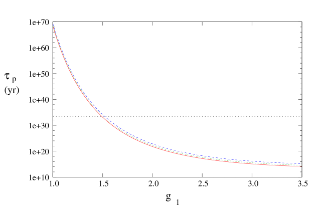
Figure 4: Proton lifetime due to $SU(2)_{1}$ instantons for $u=2$ TeV (solid red), $u=3$ TeV (dotted green), and $u=5$ TeV (dashed blue). Also shown in this figure (flat dotted line) is the $90\%$ c.l. experimental lower bound on the proton lifetime [30].

The instanton mediated proton lifetime as a function of the $SU(2)_{1}$ coupling is shown in Fig. 4. Also shown in this figure is the current experimental $90\%$ c.l. limit on proton decay via $p\to K^{+}\bar{\nu}$ [30]:

$$\tau_{p}>2.3\times 10^{33}\,yr.$$ (74)

From the figure, we see that $g_{1}\lesssim 1.5$ is required to satisfy the proton decay constraint. This upper limit on the gauge coupling $g_{1}$ puts an interesting bound on models that make use of the $SU(2)_{1}\times SU(2)_{2}$ gauge structure, such as topflavor and non-commuting extended technicolor. It also limits the amount by which the Higgs mass may be raised through $D$-terms in supersymmetric theories.

The results above were obtained for values of $u$ of the order of a few TeV. The bounds on $g_{1}$ may be relaxed by increasing the value of $u$. However, since the proton decay rate is proportional to $u^{-4}$, while it depends exponentially on the value of $g_{1}^{-2}$, a large increase on $u$ would be necessary to significantly modify the bounds on $g_{1}$. Alternatively, one can find a lower bound on $u$ for a particular value of $g_{1}$. For instance, for a value of $g_{1}\simeq 2.5$, the bound on $u$ is found to be $u\stackrel{{\scriptstyle>}}{{{}_{\sim}}}10^{8}$ GeV. The large value of the lower bound on $u$ reflects the relatively mild dependence on this parameter. We have also assumed that the effective quartic coupling for the symmetry breaking bidoublet field is small, $\lambda\ll 2\pi^{2}$. For larger values of $\lambda$, as sometimes arise in technicolor-type models [31], there will be an additional suppression of the instanton amplitude leading to a longer proton lifetime for given values of $g_{1}$ and $u$.

As we will see below, the bounds from nucleon decay are significantly weakened if there are additional fermions, beyond the third generation of the SM, that are charged under $SU(2)_{1}$. These could arise, for instance, as the superpartners of the Higgs scalars in a supersymmetric theory or from additional exotic quarks or leptons.

6 Strongly-Coupled Light Fermions

In the previous sections we have discussed the effects of instantons of the $SU(2)_{1}$ gauge group when its coupling becomes large. Since this group couples only to the third generation, one of these effects is the generation of four-fermion operators. One such operator, that of Eq. (67), leads to the rapid decay of the proton if the gauge coupling $g_{1}$ is too large. This implies an upper bound on $g_{1}$ (for a given $u$) that provides a relevant constraint on several models making use of the $SU(2)_{1}\times SU(2)_{2}$ gauge structure. This operator also generates $B+L$ violating scattering events in particle colliders, but unfortunately the cross section for these is too small to be observed at the LHC, especially given the upper bound on $g_{1}$. A second possibility, the one we consider in this section, is that the gauge coupling of the $SU(2)_{2}$ group becomes large. In this case, it is the $SU(2)_{2}$ instantons that become unsuppressed, possibly leading to observable effects.

Since the first and second generations of fermions couple to $SU(2)_{2}$, the effective operators generated by the $SU(2)_{2}$ instantons will involve eight fermions, violate $B$ and $L$ by two units each, and will be accompanied by a factor of $u^{-8}$. These operators can therefore mediate dinucleon decay, the limits on which are nearly as stringent as those for proton decay. However, because of the $u^{-8}$ factor, the decay rates will be suppressed by a factor of $(m_{p}/u)^{16}$, which is of order $10^{-50}$ for $u\sim\mbox{TeV}$. On the other hand, the scattering cross sections mediated by the instanton will go as $(\sqrt{s}/u)^{16}$. As up or a down quarks with energies of order 1 TeV can be found with non-vanishing probability at the LHC, this prefactor is not exceedingly small. Indeed, the PDF’s for valence quarks at high energies are much larger than for the bottom, which provides an additional enhancement compared to the previous case.

6.1 Di-Nucleon Decay

Using the results of Eq. (39) and Section 3, the eight-fermion operators generated by $SU(2)_{2}$ instantons will have the form

$$\mathcal{O}_{\rm{eff}} = \frac{C}{g_{2}^{8}}\,e^{-8\pi^{2}/g_{2}^{2}}\left(\frac{1}{4\pi^{2}}\right)^{b_{0}/2}2^{3+b_{0}/2}\Gamma(4+b_{0}/2)\left(\frac{\mu}{\mathcal{V}}\right)^{b_{0}}\frac{1}{\mathcal{V}^{8}}\,\tilde{\mathcal{O}},$$ (75)

$$:= \phantom{AA}\frac{\tilde{C}}{\mathcal{V}^{8}}\,\tilde{\mathcal{O}}$$

where $C$ is given in Eq. (23), and $\tilde{\mathcal{O}}$ is a linear combination of $(uude)(ccs\mu)$, $(uude)(ssc\nu_{\mu})$, $(ddu\nu_{e})(ccs\mu)$, and $(ddu\nu_{e})(ssc\nu_{\mu})$. These operators all have $B=L=2$, and can therefore induce the decay of a pair of nucleons.

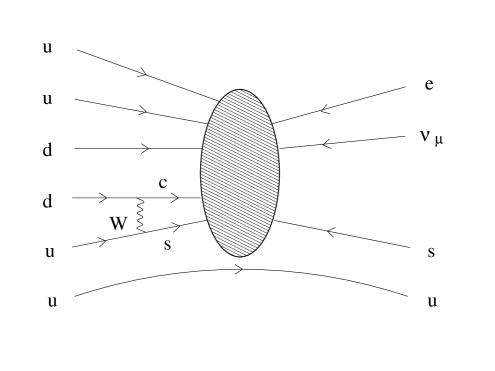
Figure 5: A Feynman diagram for diproton decay due to an $SU(2)_{2}$ instanton.

We will consider the di-proton decay rate induced by the operator $(uude)(ssc\nu_{\mu})$. The relevant Feynman diagram with the least possible number of loops is shown in Fig. 5. Calculating the amplitude for this diagram is complicated because of the nuclear physics uncertainties associated with the overlap of the proton wave functions. To make an estimate of the amplitude, we shall simply replace all unknown dimensionful terms by the proton mass $m_{p}$. This is likely a gross overestimate of the decay rate, especially since the relevant nuclear physics scale is closer to $1~{}\rm{fm}^{-1}\sim 0.2$ GeV, so our results should be considered as a robust upper bound on the actual rate. With this approximation, the di-proton lifetime is given by

$$\Gamma\simeq|\tilde{C}|^{2}\left(\frac{g}{\sqrt{2}}\right)^{4}\,\left|A(m_{c}^{2},m_{s}^{2},M_{W}^{2})\right|^{2}\,|V_{us}V^{*}_{cd}|^{2}\,\left(\frac{m_{p}}{\mathcal{V}}\right)^{16}\frac{1}{m_{p}},$$ (76)

where the function $A(a,b,c)$ was defined in Eq. (5). As for the proton decay rate, we match the effective operator at scale $\mu=\mathcal{V}$, and neglect the running below this scale.

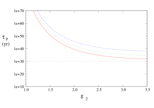
Figure 6: The di-proton lifetime induced by $SU(2)_{2}$ instantons. In this figure, the solid blue line corresponds to $u=2$ TeV, the dashed green line is for $u=3$ TeV, and the dotted blue line is for $u=5$ TeV. The flat dotted line is the current experimental lower bound.

The current best experimental limit on di-nucleon decay processes was obtained by the Fréjus collaboration, which looked for di-nucleon decay in iron, and is of the order of 10³⁰ years. The corresponding di-proton lifetime, obtained from our estimate of Eq. (76), is shown in Fig. 6. The estimated lifetime is many orders of magnitude above the experimental bound, even for very large values of the $SU(2)_{2}$ coupling. As noted above, the additional suppression relative to the $SU(2)_{1}$ case comes from the factor of $(m_{p}/\mathcal{V})^{16}$ in Eq. (76). Thus, the experimental limit on the $pp$ lifetime does not impose any strong constraint on the coupling constant $g_{2}$.

Another possible effect of the $B=L=2$ operators considered in this section are hydrogen–antihydrogen oscillations, as first suggested by Feinberg, Goldhaber and Steigman [32]. Observe that, neglecting CP-violation, the existence of $\Delta B=\Delta L=2$ interactions determines that the real mass eigenstates of Hydrogen are

$$H_{1}=\frac{1}{\sqrt{2}}\left(H\pm\bar{H}\right)$$ (77)

and will have a small mass difference. Oscillations between a pure hydrogen and antihydrogen states will occur with a period $T=2\pi/\Delta m$, that, due to astrophysical bounds must be larger than $7\times 10^{10}$ years. However, the dominant, instanton mediated process violate baryon and lepton number but also flavor. Therefore, these transitions are suppressed not only by the small instanton amplitude and $(m_{p}/\mathcal{V})^{16}$, but also by loop and mixing angle factors. A simple examination of the relevant factors involved in the baryon number violating transition suggests that the mass difference induced by the baryon number violating is much larger than the experimental bound ($T>10^{40}$ years), and is therefore unmeasurably small. Finally, we also note that neutron oscillations are not induced by the instanton operators because they also violate lepton number by two units.

6.2 Scattering by $SU(2)_{2}$ Instantons

Contrary to the case in which only one generation couples to the strongly interacting sector, the baryon number violating processes occurring in proton-proton collisions at the LHC involve six quarks and two leptons. In the following, we shall consider the scattering of two first generation quarks leading to a final state with four energetic jets and two first and second generation same-sign leptons. This is a spectacular event with very little background in the standard model, and can be easily detected when the two outgoing leptons are charged.

As in the previous subsection, the large number of fermion legs makes a precise calculation very difficult, so we will only estimate the relevant scattering cross section. In particular, we will focus on the operator $(uude)(ccs\mu)$, which can induce $uu\to\bar{d}{e}^{+}\bar{c}\bar{c}\bar{s}\mu^{+}$ at the parton level. This particular channel is the most promising one for two reasons. First, the $uu$ initial state is the most probable with respect to the PDF’s of the proton, and second, the two charged like-sign leptons in the final state produce a distinctive signature for these events. We also note that this cross section is enhanced by the fact that the LHC is a $pp$ collider, and not a $p\bar{p}$ collider such as the Tevatron, since the instanton-mediated scattering events involve two particles instead of a particle and an anti-particle.

The scattering amplitude induced by the $(uude)(ccs\mu)$ operator has the form

$$\mathcal{A}=\frac{\tilde{C}}{\mathcal{V}^{8}}\,\bar{h},$$ (78)

where $\tilde{C}$ is the factor defined in Eq. (75) and $\bar{h}$ is the matrix element of the $(uude)(ccs\mu)$ term between the external states. The cross section derived from this amplitude is

$$\sigma=\frac{1}{s}|\tilde{C}|^{2}\,\left[\prod_{i=3}^{8}\int\frac{d^{3}k_{i}}{(2\pi)^{3}2E_{i}}\right]\,(2\pi^{4})\delta^{(4)}(p_{1}+p_{2}-p_{3}-\ldots-p_{8})\,|\bar{h}|^{2},$$ (79)

in which $|\bar{h}|^{2}$ includes summation and averaging over spin and color states. To proceed, we must approximate the phase space integral. For this, we shall assume that

$$|\bar{h}|^{2}\sim\left(\frac{\sqrt{s}}{2}\right)^{2}\prod_{i=3}^{8}E_{i},$$ (80)

since in the leading term, each fermion is expected to contribute a factor of its momentum. Using the methods of [33], we find that

$$\left[\prod_{i=1}^{n}\int\frac{d^{3}k_{i}}{(2\pi)^{3}2E_{i}}\right]\,(2\pi^{4})\,\delta^{(4)}(p_{1}+p_{2}-p_{3}-\ldots-p_{8})\,\prod_{i=1}^{n}E_{i}$$ (81)

$$= \frac{1}{2}(4\pi)^{3-2n}\frac{1}{(\frac{3}{2}n-1)!(\frac{3}{2}n-2)!}s^{3n/2-2},$$

valid for large $n$. Our estimate for the (parton-level) cross section is therefore

$$\sigma=\frac{1}{s}\,|\tilde{C}|^{2}\frac{1}{8}(4\pi)^{-9}\frac{1}{7!\,8!}\left(\frac{\sqrt{s}}{\mathcal{V}}\right)^{16}.$$ (82)

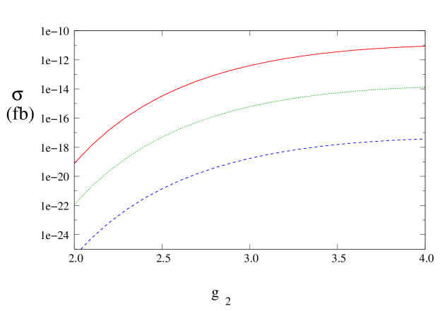
Figure 7: The instanton mediated cross section at $\sqrt{s_{0}}=14$ TeV for the case in which the first two generations are charged under the strong $SU(2)_{1}$ interactions, for three values of the scale $u=2$ TeV (solid red), 3 TeV (dotted green), and 5 TeV (dashed blue).

As in Section 4, this cross section must be convolved with the $u$ quark PDF’s in order to get the full cross section. Doing so, we find the total cross sections shown in Fig. 7 for a center-of-mass energy of $\sqrt{s_{0}}=14$ TeV. Like the cross sections due to $SU(2)_{1}$ instantons, these cross sections are too small to be observed at the LHC. Different from the $SU(2)_{1}$ case, however, the $SU(2)_{2}$ cross section is not suppressed by a small instanton prefactor ($\tilde{C}$ defined in Eq. (75) is of order unity for $g_{2}\sim 3$) or the product of bottom quark PDF’s. Instead, the very small phase space factor of Eq. (82) is responsible for inhibiting the instanton events. These results are also very sensitive to the value of $u\simeq\mathcal{V}/\sqrt{2}$ and the center of mass energy $\sqrt{s}$ due to the high power of $\mathcal{V}$ and $\sqrt{s}$ appearing in the cross section expression.

7 Conclusions

In this article we have shown that the rates of anomalous $B+L$ violating transitions in gauge extended models can be much larger than in the SM. For models based on the group $SU(2)_{1}\times SU(2)_{2}$, such as topflavor and non-commuting extended technicolor, we have found that the instanton mediated scattering cross sections are too small to be observed at the LHC, but that nucleon decay implies an upper bound on the $SU(2)_{1}$ gauge coupling. This limit is relevant for these models, and may (through dimensional deconstruction) provide a glimpse into some non-perturbative processes relevant for certain five dimensional theories. It similarly suggests that the possibility of raising the Higgs mass through $D$-terms in supersymmetric theories is limited by the bound on the $SU(2)_{1}$ gauge coupling. The opposite limit has the $SU(2)_{2}$ felt by the first and second generations to be strongly interacting. However, the instantonic effects associated with the $SU(2)_{2}$ gauge group are generally too weak to be seen, even for large values of the gauge coupling. The rate of baryon and lepton number violating processes are strongly suppressed by the small phase space factors arising in this case.

As a byproduct of this analysis, we have also re-examined the constraints on the $SU(2)_{1}\times SU(2)_{2}$ gauge structure implied by the precision electroweak data. Our results are roughly in agreement with those in the literature. In general, we find that to agree with the data, the symmetry breaking scale of the extended gauge group must be greater than a few TeV, although the limits may be relaxed in the case that only the third generation fermions are coupled to the strongly interacting gauge group.

It may be possible that other types of experiments could be sensitive to extended gauge instantons. For example, even higher energy colliders such as a VLHC will see less suppression and could have observable rates if the integrated luminosity is sufficiently high. Also, it is possible that horizontal air showers induced by cosmic neutrinos could be detected by cosmic ray observatories. Furthermore, they may open a new avenue for electroweak-style baryogenesis. While these topics are all beyond the scope of the present work, they are interesting possibilities and show that non-perturbative effects from new interactions may be just as exciting and important as the perturbative effects.

Acknowledgments

Work at ANL is supported in part by the US DOE, Div. of HEP, Contract W-31-109-ENG-38. C. Wagner would like to thank N. Weiner and S. Chivukula for useful discussions and comments. T. Tait has benefitted from discussions with B. Dobrescu and C. Hill. D. Morrissey would like to thank C. Balázs, P. Batra, and C. Hill for several helpful conversations.

Appendix A Euclidean Space Spinor Conventions

We use the following conventions in Minkowski space:

$$\eta^{\mu\nu} = diag(+1,-1,-1,-1),$$ (83)

$$\sigma^{\mu} = (\sigma^{\mu})_{\alpha\dot{\alpha}}=(\mathbb{I},\vec{\sigma}),$$

$$\bar{\sigma}^{\mu} = (\bar{\sigma}^{\mu})^{\dot{\alpha}{\alpha}}=(\mathbb{I},-\vec{\sigma}),$$

$$\sigma^{\mu\nu} = \frac{i}{4}(\sigma^{\mu}\bar{\sigma}^{\nu}-\sigma^{\nu}\bar{\sigma}^{\mu}),$$

$$\bar{\sigma}^{\mu\nu} = \frac{i}{4}(\bar{\sigma}^{\mu}{\sigma}^{\nu}-\bar{\sigma}^{\nu}{\sigma}^{\mu}).$$

In Euclidean space we take our vectors to be

$$p_{4} = -ip_{0},$$

$$p^{e}_{\mu} = (p_{i},p_{4}).$$ (84)

and define the Euclidean space $\sigma$-matrices according to

$$\sigma^{e}_{\mu} = (\vec{\sigma},i),$$ (85)

$$\bar{\sigma}^{e}_{\mu} = (\vec{\sigma},-i),$$

$$\sigma^{e}_{\mu\nu} = \frac{1}{4i}(\sigma^{e}_{\mu}\bar{\sigma}^{e}_{\nu}-\sigma^{e}_{\nu}\bar{\sigma}^{e}_{\mu}),$$

$$\bar{\sigma}^{e}_{\mu\nu} = \frac{1}{4i}(\bar{\sigma}^{e}_{\mu}{\sigma}^{e}_{\nu}-\bar{\sigma}^{e}_{\nu}{\sigma}^{e}_{\mu}).$$

This is slightly different from the conventions in Ref. [14].

With these definitions, it follows that

$$v_{\mu}w^{\mu} = -v^{e}_{\mu}w^{e}_{\mu},$$

$$v_{\mu}\sigma^{\mu} = v^{e}_{\mu}\sigma^{e}_{\mu},$$

$$v_{\mu}\bar{\sigma}^{\mu} = -v^{e}_{\mu}\bar{\sigma}^{e}_{\mu}$$

$$v_{\mu}w_{\nu}\sigma^{\mu\nu} = v^{e}_{\mu}w^{e}_{\nu}\sigma^{e}_{\mu\nu},$$ (86)

$$v_{\mu}w_{\nu}\bar{\sigma^{\mu\nu}} = v^{e}_{\mu}w^{e}_{\nu}\bar{\sigma}^{e}_{\mu\nu},$$

where repeated lower indices are summed over.

In terms of the ’t Hooft symbols, $\eta_{a\mu\nu}$, [3] we have

$$\sigma_{\mu\nu}^{e} = \bar{\eta}_{a\mu\nu}\sigma^{a}/2,$$ (87)

$$\bar{\sigma}_{\mu\nu}^{e} = {\eta}_{a\mu\nu}\sigma^{a}/2,$$

where $a=1,2,3$ is an $SU(2)$ index. The $e$’s will be left implicit in most of the expressions in this work. We will also follow the convention of Ref. [14] and use $\sigma$’s for spin-space sigma-matrices, and $\tau$’s for the $SU(2)$-space sigma-matrices.

Appendix B Gauge Bosons in the $SU(2)_{1}\times SU(2)_{2}$ Model

We list here the gauge boson masses and couplings in the $SU(2)_{1}\times SU(2)_{2}$ light and heavy gauge extensions. In both cases, the gauge coupling for the light set of weak bosons is related to the two original $SU(2)$ gauge couplings by,

$$g_{L}=\frac{g_{1}g_{2}}{\sqrt{g_{1}^{2}+g_{2}^{2}}}~{}.$$ (88)

To simplify expressions, we introduce the short-hand notation,

$$c_{\varphi}\equiv\cos\varphi = \frac{g_{1}}{\sqrt{g_{1}^{2}+g_{2}^{2}}}~{},$$ (89)

$$s_{\varphi}\equiv\sin\varphi = \frac{g_{2}}{\sqrt{g_{1}^{2}+g_{2}^{2}}}~{},$$

for the $SU(2)\times SU(2)$ gauge couplings, and

$$s_{\theta}\equiv\sin\theta = \frac{g_{y}}{\sqrt{g_{y}^{2}+g_{L}^{2}}}~{},$$ (90)

$$c_{\theta}\equiv\cos\theta = \frac{g_{L}}{\sqrt{g_{y}^{2}+g_{L}^{2}}}~{},$$

is the analog of the weak mixing angle in the SM.

B.1 The Heavy Case

The charged gauge boson states consist of $A_{j}^{\pm}=(A_{j}^{1}\mp iA_{j}^{2})/\sqrt{2}$, $j=1,2$. In this basis, the mass matrix reads

$$M_{\pm}^{2}=u^{2}\,\left(\begin{array}[]{cc}g_{1}^{2}(1+\delta)&-g_{1}g_{2}\\ -g_{1}g_{2}&g_{2}^{2}\end{array}\right),$$ (91)

where $\delta\equiv v^{2}/2u^{2}$. By assumption, $\delta\ll 1$, and we treat it as a perturbation, keeping only the terms necessary to compute the leading order in $\delta$ to EW observables.

The mass eigenstates, $W$ and $W^{\prime}$, are related to these, to $\mathcal{O}(\delta)$, by the transformation

$$\left(\begin{array}[]{c}A_{1}\\ A_{2}\end{array}\right)=\left(\begin{array}[]{cc}s_{\varphi}-s_{\varphi}c_{\varphi}^{4}\delta&-c_{\varphi}-s_{\varphi}^{2}c_{\varphi}^{3}\delta\\ c_{\varphi}+s_{\varphi}^{2}c_{\varphi}^{3}\delta&s_{\varphi}-s_{\varphi}c_{\varphi}^{4}\delta\end{array}\right)\left(\begin{array}[]{c}W\\ W^{\prime}\end{array}\right)~{}.$$ (92)

and the charged gauge boson masses are given by

$$M^{2}_{W} = \frac{g_{L}^{2}\,v^{2}}{2}\left(1-c^{4}_{\varphi}\delta\right)\;,$$ (93)

$$M^{2}_{W^{\prime}} = \frac{g_{L}^{2}\,u^{2}}{s_{\varphi}^{2}c_{\varphi}^{2}}\>=\>(g_{1}^{2}+g_{2}^{2})\,u^{2}\;{}$$

where, as above, $g_{L}=g_{1}\,g_{2}/\sqrt{g_{1}^{2}+g_{2}^{2}}$ is the gauge coupling of the diagonal $SU(2)_{L}$ subgroup.

The coupling of these gauge bosons to the fermions of the first and second generations has the form

$$g_{2}\,A_{2}\to g_{L}(1+s_{\varphi}^{2}\,c_{\varphi}^{2}\,\delta)\,W+g_{L}(\frac{s_{\varphi}}{c_{\varphi}}-s_{\varphi}c_{\varphi}^{3}\,\delta)\,W^{\prime},$$ (94)

while the coupling with the third generation fermions is given by

$$g_{1}\,A_{1}\to g_{L}(1-c_{\varphi}^{4}\,\delta)\,W+g_{L}(-\frac{c_{\varphi}}{s_{\varphi}}-s_{\varphi}c_{\varphi}^{3}\,\delta)\,W^{\prime}.$$ (95)

The mass matrix for the neutral states in basis $(B,A_{1},A_{2})$ is given by

$$M_{0}^{2}=u^{2}\,\left(\begin{array}[]{ccc}g_{y}^{2}\,\delta&-g_{1}g_{y}\,\delta&0\\ -g_{1}g_{y}\,\delta&g_{1}^{2}\left(1+\,\delta\right)&-g_{1}g_{2}\\ 0&-g_{1}g_{2}&g_{2}^{2}\end{array}\right)~{}.$$ (96)

The transformation to the mass eigenstates, $(A,Z,Z^{\prime})$ has the form

$$\left(\begin{array}[]{c}B\\ A_{1}\\ A_{2}\end{array}\right)=\left(\begin{array}[]{ccc}c_{\theta}&-s_{\theta}&\frac{s_{\theta}}{c_{\theta}}s_{\varphi}c_{\varphi}^{3}\,\delta\\ s_{\varphi}s_{\theta}&s_{\varphi}c_{\theta}-\frac{s_{\varphi}c_{\varphi}^{4}}{c_{\theta}}\,\delta&-c_{\varphi}-s_{\varphi}^{2}c_{\varphi}^{3}\,\delta\\ c_{\varphi}s_{\theta}&c_{\varphi}c_{\theta}+\frac{s_{\varphi}^{2}c_{\varphi}^{3}}{c_{\theta}}\,\delta&s_{\varphi}-s_{\varphi}c_{\varphi}^{4}\,\delta\end{array}\right)\left(\begin{array}[]{c}A\\ Z\\ Z^{\prime}\end{array}\right)~{}.$$ (97)

The masses of the $Z$ and $Z^{\prime}$ are

$${}M_{Z}^{2} = \frac{g_{L}^{2}\,v^{2}}{2\,c_{\theta}^{2}}(1-c_{\varphi}^{4}\,\delta)$$ (98)

$$M_{Z^{\prime}}^{2} = (g_{1}^{2}+g_{2}^{2})\,u^{2}.$$

The couplings of the first and second generations are

$$(g_{2}\,A_{2}t^{3}+g_{y}\,Y\,B)\>\to\>e\,Q\,A+\frac{g_{L}}{c_{\theta}}\left[(t^{3}-Q\,s_{\theta}^{2})+s_{\varphi}^{2}c_{\varphi}^{2}\delta\,t^{3}\right]\,Z+g_{L}\frac{s_{\varphi}}{c_{\varphi}}\,t^{3}\,Z^{\prime},$$ (99)

where $Q=(t^{3}+Y)$, as usual, and for the third generation we have

$$(g_{1}\,A_{1}\,t^{3}+g_{y}\,Y\,B)\>\to\>e\,Q\,A+\frac{g_{L}}{c_{\theta}}\left[(t^{3}-Q\,s_{\theta}^{2})-c_{\varphi}^{4}\delta\,t^{3}\right]\,Z-g_{L}\frac{c_{\varphi}}{s_{\varphi}}\,t^{3}\,Z^{\prime}.$$ (100)

B.2 The Light Case

The analysis of the light case is very similar to the previous section. The charged gauge boson mass matrix, in basis $(A_{1},A_{2})$, is

$$M_{\pm}^{2}=u^{2}\,\left(\begin{array}[]{cc}g_{1}^{2}&-g_{1}g_{2}\\ -g_{1}g_{2}&g_{2}^{2}(1+\delta)\end{array}\right),$$ (101)

where, again, $\delta=v^{2}/2u^{2}\ll 1$. The corresponding mixing matrix is,

$$\left(\begin{array}[]{c}A_{1}\\ A_{2}\end{array}\right)=\left(\begin{array}[]{cc}s_{\varphi}+s_{\varphi}^{3}c_{\varphi}^{2}\delta&-c_{\varphi}+s_{\varphi}^{4}c_{\varphi}\delta\\ c_{\varphi}-s_{\varphi}^{4}c_{\varphi}\delta&s_{\varphi}+s_{\varphi}^{3}c_{\varphi}^{2}\delta\end{array}\right)\left(\begin{array}[]{c}W\\ W^{\prime}\end{array}\right)~{},$$ (102)

and the charged gauge boson masses are given by

$$M^{2}_{W} = \frac{g_{L}^{2}\,v^{2}}{2}\left(1-s^{4}_{\varphi}\delta\right),$$ (103)

$$M^{2}_{W^{\prime}} = \frac{g_{L}^{2}\,u^{2}}{s_{\varphi}^{2}c_{\varphi}^{2}}\>=\>(g_{1}^{2}+g_{2}^{2})\,u^{2}\;.{}$$

The coupling of these gauge bosons to the fermions of the first and second generations has the form

$$g_{2}\,A_{2}\to g_{L}(1-s_{\varphi}^{4}\,\delta)\,W+g_{L}(\frac{s_{\varphi}}{c_{\varphi}}+s_{\varphi}^{3}c_{\varphi}\,\delta)\,W^{\prime},$$ (104)

while the coupling with the third generation fermions is given by

$$g_{1}\,A_{1}\to g_{L}(1+s_{\varphi}^{2}c_{\varphi}^{2}\,\delta)\,W+g_{L}(-\frac{c_{\varphi}}{s_{\varphi}}+s_{\varphi}^{3}c_{\varphi}\,\delta)\,W^{\prime}.$$ (105)

The mass matrix for the neutral states, in the basis $(B,A_{1},A_{2})$, is given by

$$M_{0}^{2}=u^{2}\,\left(\begin{array}[]{ccc}g_{y}^{2}\,\delta&0&-g_{2}g_{y}\,\delta\\ 0&g_{1}^{2}&-g_{1}g_{2}\\ -g_{2}g_{y}\,\delta&-g_{1}g_{2}&g_{2}^{2}\left(1+\delta\right)\end{array}\right).$$ (106)

leading to the transformation to the mass eigenstates $(A,Z,Z^{\prime})$,

$$\left(\begin{array}[]{c}B\\ A_{1}\\ A_{2}\end{array}\right)=\left(\begin{array}[]{ccc}c_{\theta}&-s_{\theta}&-\frac{s_{\theta}}{c_{\theta}}s_{\varphi}^{3}c_{\varphi}\,\delta\\ s_{\varphi}s_{\theta}&s_{\varphi}c_{\theta}+\frac{s_{\varphi}^{3}c_{\varphi}^{2}}{c_{\theta}}\,\delta&-c_{\varphi}+s_{\varphi}^{4}c_{\varphi}\,\delta\\ c_{\varphi}s_{\theta}&c_{\varphi}c_{\theta}-\frac{s_{\varphi}^{4}c_{\varphi}}{c_{\theta}}\,\delta&s_{\varphi}+s_{\varphi}^{3}c_{\varphi}^{2}\,\delta\end{array}\right)\left(\begin{array}[]{c}A\\ Z\\ Z^{\prime}\end{array}\right)~{},$$ (107)

with $Z$ and $Z^{\prime}$ masses,

$${}M_{Z}^{2} = \frac{g_{L}^{2}\,v^{2}}{2\,c_{\theta}^{2}}(1-s_{\varphi}^{4}\,\delta)$$ (108)

$$M_{Z^{\prime}}^{2} = (g_{1}^{2}+g_{2}^{2})\,u^{2}.$$

The first and second generation couplings are

$$(g_{2}\,A_{2}t^{3}+g_{y}\,Y\,B)\>\to\>e\,Q\,A+\frac{g_{L}}{c_{\theta}}\left[(t^{3}-Q\,s_{\theta}^{2})-s_{\varphi}^{4}\delta\,t^{3}\right]\,Z+g_{L}\frac{s_{\varphi}}{c_{\varphi}}\,t^{3}\,Z^{\prime}+\mathcal{O}(\delta^{2}),$$ (109)

and the third generation couplings are,

$$(g_{1}\,A_{1}\,t^{3}+g_{y}\,Y\,B)\>\to\>e\,Q\,A+\frac{g_{L}}{c_{\theta}}\left[(t^{3}-Q\,s_{\theta}^{2})+s_{\varphi}^{2}c_{\varphi}^{2}\delta\,t^{3}\right]\,Z-g_{L}\frac{c_{\varphi}}{s_{\varphi}}\,t^{3}\,Z^{\prime}+\mathcal{O}(\delta^{2}).$$ (110)

Appendix C Precision Electroweak Constraints

Using the results of the previous appendix, we perform the matching to input parameters and compute the shifts in the electroweak observables in both the heavy and light gauge-extended models. In both cases, $\alpha$ has the same form as in the SM:

$$\alpha=\frac{e^{2}}{4\,\pi}=\frac{g_{L}^{2}\,\sin^{2}\theta}{4\,\pi}~{},$$ (111)

and $g_{L}^{2}$ is given by,

$$g_{L}^{2} = \frac{4\,\pi\,\alpha}{\sin^{2}\theta}~{}.$$ (112)

C.1 Heavy Case

The expression for $M_{Z}$ is given in Eq. (98):

$$M_{Z}^{2}=\frac{g_{L}^{2}\,v^{2}}{2c^{2}_{\theta}}(1-c_{\varphi}^{4}\,\delta).$$ (113)

For $G_{F}$, which is extracted from muon decay, we must consider the low-energy effective four-fermion couplings which arise from integrating out both the $W$ and $W^{\prime}$ bosons. Using the charged gauge boson masses, Eq. (B.1), as well as their couplings to the first and second generation fermions, we find

$$4\sqrt{2}\,G_{F} = \left[\frac{g_{L}^{2}\,v^{2}}{2}\left(1-c^{4}_{\varphi}\,\delta\right)\right]^{-1}\;g_{L}^{2}(1+s_{\varphi}^{2}c_{\varphi}^{2}\,\delta)^{2}+\left[\frac{g_{L}^{2}\,u^{2}}{s_{\varphi}^{2}c_{\varphi}^{2}}\right]^{-1}\;g_{L}^{2}\left(\frac{s_{\varphi}}{c_{\varphi}}\right)^{2}$$ (114)

$$= \frac{2}{v^{2}}(1+\delta).$$

Inverting these relations, we match to our input parameters,

$$v^{2} = \frac{(1+\delta)}{2\sqrt{2}\,G_{F}}$$ (115)

$$\sin^{2}\theta = \frac{1}{2}-\frac{1}{2}\sqrt{1-4\,A_{0}[1+(1-c_{\varphi}^{4})\delta]},$$

where

$$A_{0}=\frac{\pi\,\alpha}{\sqrt{2}\,G_{F}\,M_{Z}^{2}}\simeq 0.179059~{}.$$ (116)

These are sufficient to work out the shifts in many of the electroweak observables relative to the SM. The important ones for our analysis are,

$$M_{W} = (M_{W})_{SM}\left[1-0.219(1-c_{\varphi}^{4})\delta\right]$$

$$\Gamma_{Z} = (\Gamma_{Z})_{SM}\left[1+\left(-1.348+0.790c_{\varphi}^{4}+1.684s_{\varphi}^{2}c_{\varphi}^{2}\right)\,\delta\right]$$

$$\Gamma_{had} = (\Gamma_{had})_{SM}\left[1+\left(-1.478+0.974c_{\varphi}^{4}+1.828s_{\varphi}^{2}c_{\varphi}^{2}\right)\,\delta\right]$$

$$\Gamma_{e,\mu} = (\Gamma_{e,\mu})_{SM}\left[1+\left(-1.175+1.175c_{\varphi}^{4}+2.122s_{\varphi}^{2}c_{\varphi}^{2}\right)\,\delta\right]$$

$$\Gamma_{inv} = (\Gamma_{inv})_{SM}\left[1+\left(-1.000+0.333c_{\varphi}^{4}+1.333s_{\varphi}^{2}c_{\varphi}^{2}\right)\,\delta\right]$$

$$R_{b} = (R_{b})_{SM}\left[1+\left(\>\>0.059-1.846c_{\varphi}^{4}-1.828s_{\varphi}^{2}c_{\varphi}^{2}\right)\,\delta\right]$$

$$R_{c} = (R_{c})_{SM}\left[1+\left(-0.114+0.618c_{\varphi}^{4}+0.583s_{\varphi}^{2}c_{\varphi}^{2}\right)\,\delta\right]$$

$$R_{\tau} = (R_{\tau})_{SM}\left[1+\left(-0.302+1.921c_{\varphi}^{4}+1.828s_{\varphi}^{2}c_{\varphi}^{2}\right)\,\delta\right]$$

$$R_{e,\mu} = (R_{e,\mu})_{SM}\left[1+\left(-0.302-0.201c_{\varphi}^{4}-0.293s_{\varphi}^{2}c_{\varphi}^{2}\right)\,\delta\right]$$

$$A_{b} = (A_{b})_{SM}\left[1+\left(-0.232+0.071c_{\varphi}^{4}\right)\,\delta\right]$$

$$A_{c} = (A_{c})_{SM}\left[1+\left(-1.786+1.786c_{\varphi}^{4}+1.242s_{\varphi}^{2}c_{\varphi}^{2}\right)\,\delta\right]$$

$$A_{s} = (A_{s})_{SM}\left[1+\left(-0.232+0.232c_{\varphi}^{4}+0.161s_{\varphi}^{2}c_{\varphi}^{2}\right)\,\delta\right]$$

$$A_{\tau} = (A_{\tau})_{SM}\left[1+\left(-20.391+6.215c_{\varphi}^{4}\right)\,\delta\right]$$

$$A_{e,\mu} = (A_{e,\mu})_{SM}\left[1+\left(-20.391+20.391c_{\varphi}^{4}+14.17s_{\varphi}^{2}c_{\varphi}^{2}\right)\,\delta\right]$$

$$A^{b}_{FB} = (A^{b}_{FB})_{SM}\left[1+\left(-20.621+20.462c_{\varphi}^{4}+14.17s_{\varphi}^{2}c_{\varphi}^{2}\right)\,\delta\right]$$

$$A^{c}_{FB} = (A^{c}_{FB})_{SM}\left[1+\left(-22.171+22.171c_{\varphi}^{4}+15.41s_{\varphi}^{2}c_{\varphi}^{2}\right)\,\delta\right]$$

$$A^{s}_{FB} = (A^{s}_{FB})_{SM}\left[1+\left(-20.621+20.621c_{\varphi}^{4}+14.333s_{\varphi}^{2}c_{\varphi}^{2}\right)\,\delta\right]$$

$$A^{\tau}_{FB} = (A^{\tau}_{FB})_{SM}\left[1+\left(-40.771+26.602c_{\varphi}^{4}+14.17s_{\varphi}^{2}c_{\varphi}^{2}\right)\,\delta\right]$$

$$A^{e,\mu}_{FB} = (A^{e,\mu}_{FB})_{SM}\left[1+\left(-40.771+40.771c_{\varphi}^{4}+28.34s_{\varphi}^{2}c_{\varphi}^{2}\right)\,\delta\right]$$ (117)

C.2 The Light Case

The corresponding expressions for the light case are

$$M_{Z}^{2} = \frac{g_{L}^{2}\,v^{2}}{2c_{\theta}^{2}}(1-s_{\varphi}^{4}\,\delta),$$

$$4\sqrt{2}\,G_{F} = \frac{2}{v^{2}}.$$ (118)

These translate into

$$v^{2} = \frac{1}{2\sqrt{2}\,G_{F}}$$ (119)

$$\sin^{2}\theta = \frac{1}{2}-\frac{1}{2}\sqrt{1-4\,A_{0}(1-s_{\varphi}^{4}\delta)}.$$

The corresponding shifts in the electroweak observables are

$$M_{W} = (M_{W})_{SM}\left[1+0.219s_{\varphi}^{4}\delta\right]$$

$$\Gamma_{Z} = (\Gamma_{Z})_{SM}\left[1+\left(-1.348+1.684s_{\varphi}^{2}c_{\varphi}^{2}-0.383s_{\varphi}^{4}\right)\,\delta\right]$$

$$\Gamma_{had} = (\Gamma_{had})_{SM}\left[1+\left(0.504s_{\varphi}^{2}c_{\varphi}^{2}-0.351s_{\varphi}^{4}\right)\,\delta\right]$$

$$\Gamma_{e,\mu} = (\Gamma_{e,\mu})_{SM}\left[1+\left(-0.947s_{\varphi}^{4}\right)\,\delta\right]$$

$$\Gamma_{inv} = (\Gamma_{inv})_{SM}\left[1+\left(0.667s_{\varphi}^{2}c_{\varphi}^{2}-0.333s_{\varphi}^{4}\right)\,\delta\right]$$

$$R_{b} = (R_{b})_{SM}\left[1+\left(1.787s_{\varphi}^{2}c_{\varphi}^{2}+1.770s_{\varphi}^{4}\right)\,\delta\right]$$

$$R_{c} = (R_{c})_{SM}\left[1+\left(-0.504s_{\varphi}^{2}c_{\varphi}^{2}-0.469s_{\varphi}^{4}\right)\,\delta\right]$$

$$R_{\tau} = (R_{\tau})_{SM}\left[1+\left(-1.618s_{\varphi}^{2}c_{\varphi}^{2}-1.526s_{\varphi}^{4}\right)\,\delta\right]$$

$$R_{e,\mu} = (R_{e,\mu})_{SM}\left[1+\left(0.504s_{\varphi}^{2}c_{\varphi}^{2}+0.596s_{\varphi}^{4}\right)\,\delta\right]$$

$$A_{b} = (A_{b})_{SM}\left[1+\left(0.161s_{\varphi}^{2}c_{\varphi}^{2}+0.232s_{\varphi}^{4}\right)\,\delta\right]$$

$$A_{c} = (A_{c})_{SM}\left[1+\left(0.545s_{\varphi}^{4}\right)\,\delta\right]$$

$$A_{s} = (A_{s})_{SM}\left[1+\left(0.171s_{\varphi}^{4}\right)\,\delta\right]$$

$$A_{\tau} = (A_{\tau})_{SM}\left[1+\left(14.171s_{\varphi}^{2}c_{\varphi}^{2}+20.386s_{\varphi}^{4}\right)\,\delta\right]$$

$$A_{e,\mu} = (A_{e,\mu})_{SM}\left[1+\left(6.215s_{\varphi}^{4}\right)\,\delta\right]$$

$$A^{b}_{FB} = (A^{b}_{FB})_{SM}\left[1+\left(0.161s_{\varphi}^{2}c_{\varphi}^{2}+6.450s_{\varphi}^{4}\right)\,\delta\right]$$

$$A^{c}_{FB} = (A^{c}_{FB})_{SM}\left[1+\left(6.760s_{\varphi}^{4}\right)\,\delta\right]$$

$$A^{s}_{FB} = (A^{s}_{FB})_{SM}\left[1+\left(6.286s_{\varphi}^{4}\right)\,\delta\right]$$

$$A^{\tau}_{FB} = (A^{\tau}_{FB})_{SM}\left[1+\left(14.171s_{\varphi}^{2}c_{\varphi}^{2}+26.602s_{\varphi}^{4}\right)\,\delta\right]$$

$$A^{e,\mu}_{FB} = (A^{e,\mu}_{FB})_{SM}\left[1+\left(12.431s_{\varphi}^{4}\right)\,\delta\right]$$

References

- [1] A. D. Sakharov, Pisma Zh. Eksp. Teor. Fiz. 5, 32 (1967) [JETP Lett. 5, 24 (1967 SOPUA,34,392-393.1991 UFNAA,161,61-64.1991)].
- [2] M. Gell-Mann, P. Ramond and R. Slansky, Rev. Mod. Phys. 50, 721 (1978).
- [3] G. ’t Hooft, Phys. Rev. Lett. 37, 8 (1976); G. ’t Hooft, Phys. Rev. D 14, 3432 (1976) [Erratum-ibid. D 18, 2199 (1978)].
- [4] C. T. Hill, talk given at SCGT 96, Nagoya, Nov. 13-16 1996, [arxiv:hep-ph/9702320].
-
[5]
D. J. Muller and S. Nandi,
Phys. Lett. B 383, 345 (1996)
[arXiv:hep-ph/9602390];
E. Malkawi, T. Tait and C. P. Yuan, Phys. Lett. B 385, 304 (1996) [arXiv:hep-ph/9603349];
E. Malkawi and C. P. Yuan, Phys. Rev. D 61, 015007 (2000) [arXiv:hep-ph/9906215]. - [6] R. S. Chivukula, E. H. Simmons and J. Terning, Phys. Rev. D 53, 5258 (1996) [arXiv:hep-ph/9506427].
- [7] P. Batra, A. Delgado, D. E. Kaplan and T. M. P. Tait, JHEP 0402, 043 (2004) [arXiv:hep-ph/0309149]; P. Batra, A. Delgado, D. E. Kaplan and T. M. P. Tait, JHEP 0406, 032 (2004) [arXiv:hep-ph/0404251].
- [8] M. Carena, A. Megevand, M. Quiros and C. E. M. Wagner, Nucl. Phys. B 716, 319 (2005) [arXiv:hep-ph/0410352].
- [9] C. T. Hill, S. Pokorski and J. Wang, Phys. Rev. D 64, 105005 (2001) [arXiv:hep-th/0104035]; N. Arkani-Hamed, A. G. Cohen and H. Georgi, Phys. Rev. Lett. 86, 4757 (2001) [arXiv:hep-th/0104005].
- [10] N. Arkani-Hamed and M. Schmaltz, Phys. Rev. D 61, 033005 (2000) [arXiv:hep-ph/9903417]; G. R. Dvali and M. A. Shifman, Phys. Lett. B 475, 295 (2000) [arXiv:hep-ph/0001072]; D. E. Kaplan and T. M. P. Tait, JHEP 0006, 020 (2000) [arXiv:hep-ph/0004200]; D. E. Kaplan and T. M. P. Tait, JHEP 0111, 051 (2001) [arXiv:hep-ph/0110126].
- [11] C. Csaki and H. Murayama, Nucl. Phys. B 532, 498 (1998) [arXiv:hep-th/9804061].
- [12] H. Aoyama and H. Goldberg, Phys. Lett. B 188, 506 (1987).
- [13] A. Ringwald, Nucl. Phys. B 330, 1 (1990).
- [14] O. Espinosa, Nucl. Phys. B 343, 310 (1990).
- [15] L. D. McLerran, A. I. Vainshtein and M. B. Voloshin, Phys. Rev. D 42, 171 (1990); J. M. Cornwall, Phys. Lett. B 243, 271 (1990); P. B. Arnold and M. P. Mattis, Phys. Rev. D 42, 1738 (1990); S. Y. Khlebnikov, V. A. Rubakov and P. G. Tinyakov, Nucl. Phys. B 347, 783 (1990); S. Y. Khlebnikov, V. A. Rubakov and P. G. Tinyakov, Nucl. Phys. B 350, 441 (1991); A. H. Mueller, Nucl. Phys. B 348, 310 (1991); A. H. Mueller, Nucl. Phys. B 353, 44 (1991)A. Ringwald and C. Wetterich, Nucl. Phys. B 353, 303 (1991)M. Maggiore and M. A. Shifman, Nucl. Phys. B 371, 177 (1992): V. V. Khoze, J. Kripfganz and A. Ringwald, Phys. Lett. B 275, 381 (1992) [Erratum-ibid. B 279, 429 (1992)]; V. V. Khoze, J. Kripfganz and A. Ringwald, Phys. Lett. B 277, 496 (1992); A. Ringwald, Phys. Lett. B 285, 113 (1992); V. A. Rubakov, D. T. Son and P. G. Tinyakov, Phys. Lett. B 287, 342 (1992); D. Diakonov and V. Petrov, Phys. Rev. D 50, 266 (1994) [arXiv:hep-ph/9307356]; F. Bezrukov, C. Rebbi, V. A. Rubakov and P. Tinyakov, arXiv:hep-ph/0110109.
- [16] V. I. Zakharov, Nucl. Phys. B 371, 637 (1992); M. Porrati, Nucl. Phys. B 347, 371 (1990); V. V. Khoze and A. Ringwald, Nucl. Phys. B 355, 351 (1991); V. V. Khoze and A. Ringwald, Phys. Lett. B 259, 106 (1991).
- [17] E. V. Shuryak and J. J. M. Verbaarschot, Phys. Rev. Lett. 68, 2576 (1992).
- [18] G. R. Farrar and R. b. Meng, Phys. Rev. Lett. 65, 3377 (1990); A. Ringwald, F. Schrempp and C. Wetterich, Nucl. Phys. B 365, 3 (1991); M. J. Gibbs, A. Ringwald, B. R. Webber and J. T. Zadrozny, Z. Phys. C 66, 285 (1995) [arXiv:hep-ph/9406266]; M. J. Gibbs and B. R. Webber, Comput. Phys. Commun. 90, 369 (1995) [arXiv:hep-ph/9504232].
- [19] F. Bezrukov, D. Levkov, C. Rebbi, V. A. Rubakov and P. Tinyakov, Phys. Rev. D 68, 036005 (2003) [arXiv:hep-ph/0304180]; F. Bezrukov, D. Levkov, C. Rebbi, V. A. Rubakov and P. Tinyakov, Phys. Lett. B 574, 75 (2003) [arXiv:hep-ph/0305300].
- [20] For reviews, see: M. P. Mattis, Phys. Rept. 214, 159 (1992); V. A. Rubakov and M. E. Shaposhnikov, Usp. Fiz. Nauk 166, 493 (1996) [Phys. Usp. 39, 461 (1996)] [arXiv:hep-ph/9603208]; A. Ringwald, Phys. Lett. B 555, 227 (2003) [arXiv:hep-ph/0212099].
- [21] S. Eidelman et al. [Particle Data Group Collaboration], Phys. Lett. B 592, 1 (2004).
- [22] [LEP Collaborations], constraints on the arXiv:hep-ex/0412015; K. Matchev, arXiv:hep-ph/0402031.
- [23] I. Affleck, Nucl. Phys. B 191, 429 (1981).
- [24] E. D’Hoker and E. Farhi, Nucl. Phys. B 241, 109 (1984).
- [25] C. Hill, talk given at the MCTP Top Quark Symposium, April 7-8, 2005, Ann Arbor, Michigan. (http://www.umich.edu/ mctp/events/topquark/HILL.PPT)
- [26] For an interesting review, J. Terning, arXiv:hep-th/0306119.
- [27] H. Lehmann, K. Symanzik and W. Zimmermann, Nuovo Cim. 1, 205 (1955).
- [28] J. Pumplin, D. R. Stump, J. Huston, H. L. Lai, P. Nadolsky and W. K. Tung, JHEP 0207, 012 (2002) [arXiv:hep-ph/0201195];
- [29] S. Aoki et al. [JLQCD Collaboration], Phys. Rev. D 62, 014506 (2000) [arXiv:hep-lat/9911026].
- [30] K. Kobayashi et al. [Super-Kamiokande Collaboration], arXiv:hep-ex/0502026.
- [31] C. T. Hill and E. H. Simmons, Phys. Rept. 381, 235 (2003) [Erratum-ibid. 390, 553 (2004)] [arXiv:hep-ph/0203079].
- [32] G. Feinberg, M. Goldhaber and G. Steigman, Phys. Rev. D 18, 1602 (1978); L. Arnellos and W. J. Marciano, Phys. Rev. Lett. 48, 1708 (1982).
- [33] E. Byckling and K. Kajantie, Particle Kinematics, Wiley-Interscience, London UK (1973).