Extraction of the $K\bar{K}$ isovector scattering length from $pp\to dK^{+}\bar{K}^{0}$ data near threshold

Abstract

The results of a recent experiment measuring the reaction $pp\to dK^{+}\bar{K}^{0}$ near threshold are interpreted in terms of a spectator model that encapsulates the main features of the observed $K^{+}\bar{K}^{0}$ invariant mass distribution. A $\chi^{2}$ fit to this data leads to an imaginary part of the isovector scattering length in the $K\bar{K}$ channel of $Im(a_{1})=-(0.63\pm 0.24)$ fm. We then use the Flatté representation of the scattering amplitude to infer a value $Re(a_{1})=-(0.02\pm 0.02)$ fm for the real part under the assumption that scaling (Baru et al.Baru05 ) is approximately satisfied. We show further that it is not possible to exclude the effects of $\pi^{+}\eta$ to $K^{+}\bar{K}^{0}$ channel coupling within the context of our model.

PACS numbers: 13.75.-n, 14.40.Cs, 25.40.Ve

Corresponding author: R H Lemmer

Electronic address: rh_-lemmer@mweb.co.za

.1 1. Introduction

The reaction $pp\to dK^{+}\bar{K}^{0}$ has been measured at an excess energy of $Q$ = $46$ MeV with the spectrometer ANKE at the cooler synchrotron COSY-JülichVK03 . This experiment has achieved a resolution of $1-8$ MeV for the invariant mass–spectrum of the $K\bar{K}$ system which considerably improves the data base. Therefore it is timely to investigate what information regarding the $K\bar{K}$ scattering length can be extracted from this data.

A model-independent analysis of the angular distributions shows a dominance of an $s$ wave between the two kaons accompanied by a $p$ wave deuteron with respect to the mesons. This has been interpreted as evidence for a dominant production of the $a_{0}(980)$ near threshold VK03 ; HANHART04 . Detailed calculations of the reaction $pp\to dK^{+}\bar{K}^{0}$ performed by Grishina et al.GRISHINA04 confirm this conclusion. In particular the non–resonant $K^{+}\bar{K}^{0}$ production is shown to be small below excess energies of $Q$ = $100$ MeV. Fadeev calculations for the $K^{-}d$ reaction have extracted a scattering length $a_{K^{-}d}=(1.80-i1.55)$ fm (using the Bethe sign convention here)Bah03 . A summary of $K^{-}d$ scattering lengths obtained by different authors can be found in Ref.SIBIRTSEV04 with $Re(a_{K^{-}d})$ ranging from $0.01$ to $1.92$ fm.

Data obtained more recently at COSY have been analysed by Sibirtsev et al. SIBIRTSEV04 . These authors have extracted limits for the $\bar{K}d$ scattering length from the data of Ref. VK03 and found the magnitudes of both the real and imaginary parts of this quantity to be less than $1.3$ fm. A chiral approach to the reaction $pp\to dK^{+}\bar{K}^{0}$ has been formulated by Oset, Oller and Meissner OSET01 that suggests a potentially large sensitivity of the data to the $\bar{K}d$ scattering length. A study FELIX05 based on this formalism finds an optimal fit to the COSY data for a purely imaginary $\bar{K}d$ scattering length of $a_{\bar{K}d}$ = $(0.0+i1.0)$ fm.

The finding of a small real part of the scattering length $a_{\bar{K}d}$ in Refs.SIBIRTSEV04 ; FELIX05 encourages us to explore the working assumption that the deuteron’s role is simply that of a spectator, and that the $K^{+}\bar{K}^{0}$ production in $pp\to dK^{+}\bar{K}^{0}$ is dominated by final state interactions in the meson–meson channels. Since the reaction $pp\to d\pi^{+}\eta$ has a lower threshold than $pp\to dK^{+}\bar{K}^{0}$, both $\pi^{+}\eta$ production and $K^{+}\bar{K}^{0}$ production have to be treated simultaneously. We therefore consider a coupled channel description of the two–meson final states $\pi^{+}\eta$ and $K^{+}\bar{K}^{0}$. In the vicinity of the $K^{+}\bar{K}^{0}$ threshold, one expects the $\pi^{+}\eta$ production to dominate. This allows one to make a simple estimate of the two kaon production via the chain $\pi^{+}\eta\to a^{+}_{0}\to K^{+}\bar{K}^{0}$. In order to include the other reaction chain $K^{+}\bar{K}^{0}\to a^{+}_{0}\to K^{+}\bar{K}^{0}$, one would need a model for the production operators. In view of this we assume that the first reaction chain is dominant, but explore the influence of the second chain empirically. This approach cannot make any predictions about the three additional measured angular distributions or the $d\bar{K}^{0}$ invariant mass distribution reported in Ref.VK03 .

.2 2. Spectator model calculation

The scattering amplitudes for $K^{+}\bar{K}^{0}\to K^{+}\bar{K}^{0}$ and $\pi^{+}\eta\to K^{+}\bar{K}^{0}$ are related by two–channel unitarity. Therefore at low relative momentum $k$ in the two kaon channel both amplitudes can be expressed in terms of the $K\bar{K}$ isovector complex scattering length $a_{1}=\alpha_{s}-i\beta_{s}$. Calling these two channels $1$ and $2$ respectively, one has COHEN80

$$T_{11}=\eta\;e^{2i\delta_{1}}-1\approx-2ika_{1}(1-ika_{1})$$

$$e^{-i\delta_{12}}T_{12}=i\sqrt{1-\eta^{2}}\approx 2i\sqrt{\beta_{s}k}(1-\beta_{s}k)$$ (1)

where $\delta_{1,2}$ are the phase shifts in the corresponding channels, $\delta_{12}=\delta_{1}+\delta_{2}$, and $\eta$ is the inelasticity.

We now assume that the $s$ wave single differential cross section $d\sigma^{(s)}/dP_{0}$ for the $pp\to dK^{+}\bar{K}$ three–body decay can be written as the proportionality

$$d\sigma^{(s)}/dP_{0}\sim\int_{t_{min}}^{t_{max}}dt|AT_{12}+BT_{11}|^{2}\approx C_{s}k|(1-\beta_{s}k)+\rho e^{i\phi}\sqrt{\beta_{s}k}\;|^{2}\Delta t$$ (2)

where $\rho\;exp(i\phi)=iB/A(1+i\alpha_{s}/\beta_{s})\;exp(-i\delta_{12})$ summarizes the admixture of channel $1$ via the ratio of the production operators $A$ and $B$ for channels $1$ and $2$, $\Delta t$ is equal to the difference in limits of the phase space integration,

$$\Delta t=t_{max}-t_{min}\sim\sqrt{(s-(m_{D}+P_{0})^{2})(s-(m_{D}-P_{0})^{2})},$$ (3)

$s=(p_{A}+p_{B})^{2}$ is the invariant mass of the colliding protons, and $C_{s}$ a coefficient of proportionality. In principle both $C_{s}$ and $\rho\;exp(i\phi)$ will depend on specific details and kinematics of the production mechanism in the two channels in question. We assume these factors to be slowly–varying for simplicity. For the three–body collision the $K\bar{K}$ invariant mass is restricted to the range from threshold $(P_{0})_{min}=(M_{K^{+}}+M_{\bar{K}^{0}})$ to $(P_{0})_{max}=(\sqrt{s}-m_{D})$ so that $\Delta t$ vanishes at the upper limit; $m_{D}$ is the deuteron mass. At the COSY proton beam energy of $T_{p}=2.65$ GeV ($p_{p}=3.46$ GeV/c) at which the experiment was performed, these limits are $(P_{0})_{min}=0.9914$ GeV and $(P_{0})_{max}=1.038$ GeV resp. This restricts the $K^{+}\bar{K}^{0}$ and $\pi^{+}\eta$ CM momenta,

$$k=\frac{1}{2}P_{0}\Big{[}1-\frac{(M_{K^{+}}-M_{\bar{K}^{0}})^{2}}{P^{2}_{0}}\Big{]}^{1/2}\Big{[}1-\frac{(M_{K^{+}}+M_{\bar{K}^{0}})^{2}}{P^{2}_{0}}\Big{]}^{1/2}$$

$$p=\frac{1}{2}P_{0}\Big{[}1-\frac{(M_{\pi}-M_{\eta})^{2}}{P^{2}_{0}}\Big{]}^{1/2}\Big{[}1-\frac{(M_{\pi}+M_{\eta})^{2}}{P^{2}_{0}}\Big{]}^{1/2}$$ (4)

to lie in the very limited intervals $0<k<0.15$ GeV and $0.33<p<0.36$ GeV respectively. The $P_{0}$ dependence of the cross section is thus completely determined by the variation of $k$ and $\Delta t$ with $P_{0}$ as fixed by Eqs. (4) and (3). The scale constant $C_{s}[\mu b\;GeV^{-4}]$ controls the absolute value of the $s$–wave cross section while the parameter $\beta_{s}=-Im(a_{1})$ determines its skewness in the case of no admixture, $\rho=0$.

The expression equivalent to Eq. (2) for $p$ waves to leading order in $k$ is

$$d\sigma^{(p)}/dP_{0}\approx C_{p}k^{3}\Delta t$$ (5)

which for $C_{p}=150.6\mu b\;GeV^{-6}$ reproduces the corresponding contribution determined in VK03 .

The fits to the various data shown in Ref.VK03 employ a six–parameter transition matrix fits ; VC02 fitted simultaneously to the two invariant mass distributions $K^{+}\bar{K}^{0}$ and $d\bar{K}^{0}$, plus three angular distributions. In order to compare the cross section given by the spectator model with their result for the $K^{+}\bar{K}^{0}$ invariant mass distribution, we have determined the pair of $s$ wave constants $[C_{s},\beta_{s}]$ by performing a $\chi^{2}$ fit to the data points in Fig. 1 that lie above threshold, using the sum of Eqs. (2) and (5) after expanding the former up to order ${\cal O}(k)$, initially for the case of no mixing, $\rho=0$. In Sect.4 we discuss the effect of including channel admixtures as well as relaxing the assumptions on $C_{s}$.

One finds $C_{s}=22.03\mu b\;GeV^{-4}$, together with an imaginary part of the scattering length of $\beta_{s}=Im(-a_{1})=0.63$ fm at $\chi^{2}_{min}=0.65$. The fit to experiment for this parameter set is shown in Fig. 1. By integrating out over the allowed range of $P_{0}$, one obtains a total cross section of $\sigma(pp\to dK^{+}\bar{K}^{0})=36$ nb, in agreement with the experimental cross section [$38\pm 2(stat)\pm 14(syst)]$ nb reported in VK03 .

.3 3. Flatté parametrization for scattering length

The spectator model assumption Eq. (2) can only fix the imaginary part of the scattering length for given [$\rho,\phi$]: it does not allow one to extract the real part directly. In order to make further progress one therefore has to introduce specific model dependent assumptions regarding the structure of the $K\bar{K}$ scattering amplitude in the isovector channel that describe the formation and decay of the $a_{0}(980)$.

There is little experimental information available on the $K\bar{K}$ scattering length. However, within the last decade the production of $\pi\eta$ pairs have been studied experimentally in proton–antiproton annihilation, pion–proton reactions and in $\Phi$ decay, and analysed using either Flatté distributionsNNA03 ; AAl02 ; ST99 ; MNA00 , or other approachesDVB94 ; OBELIX03 ; AA98 . The Flatté scattering amplitudeflatte76 near the $K\bar{K}$ threshold takes on the form

$$S_{K\bar{K}}\approx 1-\frac{i\bar{g}_{K\bar{K}}k}{-\epsilon_{a_{0}}+\frac{i}{2}(\bar{g}_{K\bar{K}}k+\bar{g}_{\pi\eta}p)}$$ (6)

where $k$ and $p$ are the CM momenta defined in Eqs. (4), while the $a_{0}(980)$ partial decay widths $\Gamma_{\pi\eta}=\bar{g}_{\pi\eta}p$ and $\Gamma_{K\bar{K}}=\bar{g}_{K\bar{K}}k$ define the dimensionless coupling constants ($\bar{g}_{\pi\eta},\bar{g}_{K\bar{K}}$); $\epsilon_{a_{0}}=M_{a_{0}}-(M_{K^{+}}+M_{\bar{K}^{0}})$ is the (real or virtual) binding energy of the $a_{0}(980)$ relative to the $K\bar{K}$ threshold. Eq. (6) leads to the following result for the $K\bar{K}$ isovector scattering lengthBM04

$$a_{1}=\frac{\frac{1}{2}\bar{g}_{K\bar{K}}}{-\epsilon_{a_{0}}+\frac{i}{2}\Gamma_{\pi\eta}}=\frac{R}{-\alpha+i}p^{-1}_{th}$$ (7)

when rewritten in terms of the dimensionless ratiosBaru05 $R=\bar{g}_{K\bar{K}}/\bar{g}_{\pi\eta}$ and $\alpha=2\epsilon_{a_{0}}/\Gamma_{\pi\eta}$ instead of the individual coupling constants and energy parameters. Here $p_{th}=p[(P_{0})_{min}]=0.33$ GeV = $1.65$ fm^-1 is the threshold momentum for $K\bar{K}$ production in the $\pi\eta$ channel.

The $R$ and $\alpha$ are seen to be invariant under a scaling $\bar{g}_{K\bar{K}}\to\lambda\bar{g}_{K\bar{K}}$ etc. of the original Flatté parameters. Table I shows a compendium of mass, width and coupling constant values for $a_{0}(980)$ taken from the recent literatureNNA03 ; AAl02 ; ST99 ; MNA00 ; DVB94 ; OBELIX03 ; AA98 and as partially summarised in BM04 ; Baru05 . We have also used Eq. (7) to extend the calculations given in BM04 for the scattering lengths associated with these paramaters. The results are displayed in order of increasing $\alpha$ in Table I.

From Eq. (7) one sees that there is a linear relation between the real and imaginary parts of the (Flatté) scattering lengths,

$$Re(-a_{1})=Im(-a_{1})\alpha$$ (8)

If we now take $Im(-a_{1})=0.63$ fm from the spectator model fit, this fixes the slope of the straight line in Eq. (8). The result can then be compared with the values of $Re(-a_{1})$ calculated from Eq. (7) at the values of $\alpha$ and $R$ given in Table I. This comparison is shown in Fig. 2. The spectator model result is seen to be consistent with all of the data (except perhaps that of Ref. OBELIX03 ) once the uncertainties in $\alpha$ and hence $Re(-a_{1})$ due to the experimental error in the $a_{0}(980)$ mass are taken into consideration.

It has also been pointed outBaru05 that direct measurements of the $K\bar{K}$ elastic scattering cross section near threshold would serve to determine both $R$ and $\alpha$ independently, and thus the scattering length as given by Eq. (7). Such data is not available yet. However, by assuming that scale invariance is valid, one can infer a value for $\alpha$ to be used in Eq. (8) by arguing as follows: the combinations $\alpha$ in Table I would have appeared as a common constant $\alpha_{c}$ had the data satisfied scaling exactly. It is therefore reasonable to estimate this unknown constant by the mean of the $\alpha$’s given in Table I, weighted by the inverse of the average error introduced into each $\alpha$ by the uncertainty in the $a_{0}(980)$ mass value used to calculate it. The resultant mean and its standard deviation is then $\alpha_{c}=0.031\pm 0.054$. By also considering the changes in slope of the linear relation Eq.(8) due to the errors introduced into $Re(-a_{1})$ by the mass value uncertainty one obtains the order of magnitude estimate $\beta_{s}=(0.63\pm 0.24$) fm for the error in $\beta_{s}$. Inserting these values for $\beta_{s}$ and $\alpha_{c}$ together with their estimated errors into Eq. (8) gives

$$a_{1}\approx-[(0.02\pm 0.02)+i(0.63\pm 0.24)]{\rm fm}$$ (9)

for the isovector scattering length.

Note that this result relies on two very different sources of information: (i) a direct determination of $Im(a_{1})$ based on the spectator model fit of the $pp\to dK^{+}\bar{K}^{0}$ data for $\rho=0$, and (ii), an inferred estimate of $Re(a_{1})$ based on the assumption that scaling is approximately valid for the experimental parameters extracted assuming a Flatté distribution.

.4 4. Effect of mixing with $K^{+}\bar{K}^{0}\to K^{+}\bar{K}^{0}$

We now repeat the $\chi^{2}$ fit of the data points in Fig. 1 in the presence of mixing. Since $\rho>1$ can lead to unphysical values of $\beta_{s}<0$, we illustrate the effects of mixing for the two limiting cases labelled $[\rho,\phi]$ = $[1,\pi]$ and $[1,0]$ in Fig. 2. The corresponding values of $\beta_{s}$ swing from $0.21$ to $7.6$ fm respectively as illustrated by the gradients of these two straight lines. However, by choosing an intermediate value of $\phi$ appropriately in the interval $0\leq\phi\leq\pi$ for given $\rho$, in this case $[\rho,\phi]=[1,110^{0}\pm 8^{0}]$, one again recovers a fit ($\chi^{2}_{min}=0.82$) to the data in Fig.1 at the indicated value of $\beta_{s}$ given in Eq. (9) that is essentially indistinguishable from the no–mixing case. Similar observations hold for any $0<\rho<1$ except that the swing in possible values of $\beta_{s}$ is smaller.

Another source of uncertainty is associated with the lack of a detailed description of the production mechanism itself. As an illustration of this we compare with the specific model for the production mechanism suggested in Ref.VC02 that codifies selection rules explicitly. One finds that their scattering amplitude, which also considers resonance production, reduces to the first term of Eq. (2) at low momentum with $C_{s}\to(C^{{}^{\prime}}_{s}p^{2}_{D})$, where $p_{D}$ is the deuteron momentum. Making this replacement in Eq. (2), one obtains an equally good fit $(\chi^{2}_{min}=0.20)$ of the mass distribution in Fig.1 with $\beta_{s}=0.63$ fm by changing the mixing angle from $110^{0}$ to $59^{0}\pm 4^{0}$.

At the level of the spectator model as envisaged in this note it is therefore impossible to decide whether or not channel mixing is important without introducing model specific assumptions for the production operators $A$ and $B$.

.5 Acknowledgments

We would like to thank the Ernest Oppenheimer Memorial Trust for research support in the form of a Harry Oppenheimer Fellowship. Thanks are also due to the Institut für Kernphysik, Forschungszentrum, Jülich, and the Max–Planck–Institut für Kernphysik, Heidelberg for their kind hospitality. Discussions with M. Büscher and S. Krewald are gratefully acknowledged.

.6 References

(^‡) Permanent address: School of Physics, University of the Witwatersrand, Johannesburg,
Private Bag 3, WITS 2050, South Africa.

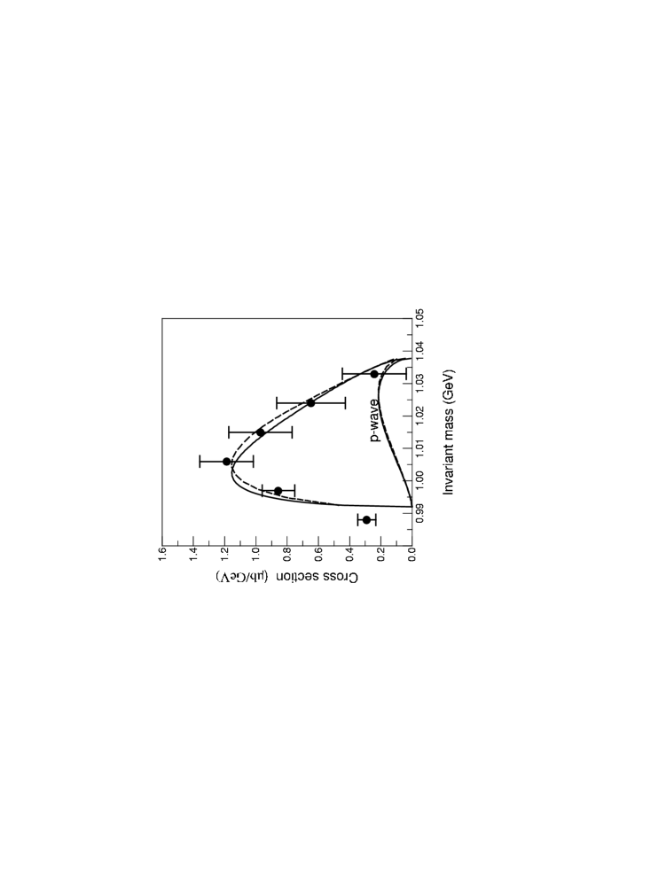
Figure 1: The invariant mass cross section for the production of $K^{+}\bar{K}^{0}$ in $pp\to dK\bar{K}$. The solid line denotes a $\chi^{2}$ fit to the dataVK03 using the spectator model without mixing (the $\chi^{2}$ fits in the presence of mixing are essentially identical for reasonable choices of the mixing parameters $[\rho,\phi]$). The broken curve shows the corresponding fit calculated in VK03 using a six–parameter transition amplitude squared. Shown separately are the $p$ wave contributions to the cross section obtained from Eq. (5) (solid curve), and the fit (broken curve) given in VK03 . The error bars show the statistical uncertainties of the data.

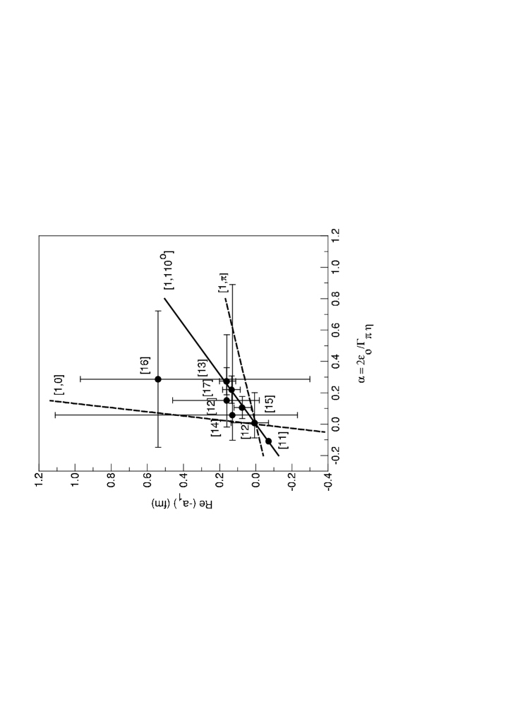
Figure 2: Plot of $Re(-a_{1})$ (filled circles) versus the dimensionless parameter $\alpha=2\varepsilon_{0}/\Gamma_{\pi\eta}$. The plotted points have been tagged by the corresponding references in Table I. The horizontal and vertical error bars show the errors introduced into $\alpha$, and hence $Re(-a_{1})$, by the uncertainties in the associated $a_{0}(980)$ mass values. The heavy straight line shows the calculated value of $Re(-a_{1})$ using Eq. (8) with $\beta_{s}=Im(-a_{1})=0.63$ fm. The label $[1,110^{0}]$ gives the mixing parameters that lead to the same value of $\beta_{s}$ upon including channel mixing as characterised by the parameters $[\rho,\phi]$ defined in the text, while the remaining two broken straight lines labelled $[1,\pi]$ and $[1,0]$ show the minimum and maximum values that $\beta_{s}$ can assume for $\rho=1$.

Table 1: Summary of calculated values of the isovector scattering length $a_{1}$ taken from Eq. (7), arranged in order of increasing $\alpha=2\varepsilon_{0}/\Gamma_{\pi\eta}$, for the various mass, width and coupling constants for the $a_{0}(980)$ as extractedBaru05 from the literature.

$Ref.$	$M_{a_{0}}$ (MeV)	$\varepsilon_{a_{0}}$ (MeV)	$\Gamma_{\pi\eta}$ (MeV)	$\bar{g}_{\pi\eta}$	$\bar{g}_{K\bar{K}}$	$R$	$\alpha$	$a_{1}$ (fm)
AAl02	$984.8^{+1.2}_{-1.2}$	$-6.6$	$121.5$	$0.373$	$0.412$	$1.10$	$-0.108$	$+0.071-0.66i$
NNA03	$992^{+14}_{-7}$	$0.6$	$145.3$	$0.446$	$0.560$	$1.252$	$0.008$	$-0.006-0.76i$
MNA00	$995^{+52}_{-10}$	$3.6$	$125$	$0.384$	$1.414$	$3.685$	$0.058$	$-0.13-2.23i$
DVB94	$999^{+5}_{-5}$	$7.6$	$143$	$0.439$	$0.516$	$1.176$	$0.106$	$-0.075-0.70i$
NNA03	$1003^{+32}_{-13}$	$11.6$	$153$	$0.470$	$0.834$	$1.776$	$0.152$	$-0.16-1.05i$
AA98	$999^{+3}_{-3}$	$7.6$	$69$	$0.212$	$0.222$	$1.048$	$0.220$	$-0.13-0.61i$
ST99	$1001^{+3}_{-3}$	$9.6$	$70$	$0.215$	$0.224$	$1.043$	$0.274$	$-0.16-0.59i$
OBELIX03	$998^{+10}_{-10}$	$6.6$	$46$	$0.141$	$0.476$	$3.376$	$0.287$	$-0.54-1.89i$

References

- (1) V. Kleber et al., Phys. Rev. Lett. 91, (2003) 172304–1.
- (2) C. Hanhart, Phys. Rep. 397, (2004) 155.
- (3) V. Yu. Grishina et al., Eur. Phys. J. A21, (2004) 507.
- (4) A. Bahaoui, C. Fagard, T. Mitzutani and B. Saghai, Phys. Rev. C68, (2003) 064001.
- (5) A. Sibirtsev et al., Phys. Lett. B601, (2004) 132.
- (6) E. Oset, J. A. Oller and U. G. Meissner, Eur. Phys. J. A12, (2001) 435.
- (7) F. P. Sassen, PhD dissertation, University of Bonn (2004); to be published.
- (8) D. Cohen et al., Phys. Rev.D22, (1980) 2595.
- (9) V. Yu. Grishina et al., Phys. Lett. B 521, (2001) 217; A. E. Kudryavtsev et al., Phys. Rev. C 66, (2002) 015207.
- (10) V. Chernyshev et al., nucl–th/0110069.
- (11) A. Aloisio et al. (The KLOE Collaboration), Phys. Lett. B536, (2002) 209.
- (12) N. N. Achasov and A. N. Kiselev, Phys. Rev. D 68, (2003) 014006.
- (13) S. Teige et al., Phys. Rev. D 59, (1999) 021001.
- (14) M. N. Achasov et al., Phys. Lett. B479, (2000) 53.
- (15) D. V. Bugg, V. V. Anisovich, A. Sarantsev, and B. S. Zou, Phys. Rev. D 50, (1994) 4412.
- (16) M. Bargiotti et al. (The OBELIX Collaboration), Eur. Phys. J C 26, (2003) 371.
- (17) A. Abele, et al., Phys. Rev. D 57, (1998) 3860.
- (18) S. Flatté, Phys. Lett. 63B, (1976) 224.
- (19) V. Baru et al., Phys. Lett. B 586, (2004) 53.
- (20) V. Baru, J. Haidenbauer, C. Hanhart, A. Kudryavtsev, and U. G. Meissner, Eur. Phys. J. A23, (2005) 523.