November, 2005

Charmless hadronic $B$ decays involving scalar mesons:

Implications to the nature of light scalar mesons

Hai-Yang Cheng¹, Chun-Khiang Chua¹ and Kwei-Chou Yang²

¹ Institute of Physics, Academia Sinica

Taipei, Taiwan 115, Republic of China

² Department of Physics, Chung Yuan Christian University

Chung-Li, Taiwan 320, Republic of China

Abstract

The hadronic charmless $B$ decays into a scalar meson and a pseudoscalar meson are studied within the framework of QCD factorization. Based on the QCD sum rule method, we have derived the leading-twist light-cone distribution amplitudes of scalar mesons and their decay constants. Although the light scalar mesons $f_{0}(980)$ and $a_{0}(980)$ are widely perceived as primarily the four-quark bound states, in practice it is difficult to make quantitative predictions based on the four-quark picture for light scalars. Hence, predictions are made in the 2-quark model for the scalar mesons. The short-distance approach suffices to explain the observed large rates of $f_{0}(980)K^{-}$ and $f_{0}(980)\overline{K}^{0}$ that receive major penguin contributions from the $b\to ss\bar{s}$ process. When $f_{0}(980)$ is assigned as a four-quark bound state, there exist extra diagrams contributing to $B\to f_{0}(980)K$. Therefore, a priori the $f_{0}(980)K$ rate is not necessarily suppressed for a four-quark state $f_{0}(980)$. The predicted $\overline{B}^{0}\to a_{0}^{\pm}(980)\pi^{\mp}$ and $a_{0}^{+}(980)K^{-}$ rates exceed the current experimental limits, favoring a four-quark nature for $a_{0}(980)$. The penguin-dominated modes $a_{0}(980)K$ and $a_{0}(1450)K$ receive predominant weak annihilation contributions. There exists a two-fold experimental ambiguity in extracting the branching ratio of $B^{-}\to\overline{K}_{0}^{*0}(1430)\pi^{-}$, which can be resolved by measuring other $K_{0}^{*}(1430)\pi$ modes in conjunction with the isospin symmetry consideration. Large weak annihilation contributions are needed to explain the $K^{*}_{0}(1430)\pi$ data. The decay $\overline{B}^{0}\to\kappa^{+}K^{-}$ provides a nice ground for testing the 4-quark and 2-quark nature of the $\kappa$ meson. It can proceed through $W$-exchange and hence is quite suppressed if $\kappa$ is made of two quarks, while it receives a tree contribution if $\kappa$ is predominately a four-quark state. Hence, an observation of this channel at the level of ${\ \lower-1.2pt\vbox{\hbox{\hbox to0.0pt{$>$\hss}\lower 5.0pt\vbox{\hbox{$\sim$} }}}\ }10^{-7}$ may imply a four-quark assignment for the $\kappa$. Mixing-induced CP asymmetries in penguin-dominated modes are studied and their deviations from $\sin 2\beta$ are found to be tiny.

I Introduction

The first charmless $B$ decay into a scalar meson that has been observed is $B\to f_{0}(980)K$. It was first measured by Belle in the charged $B$ decays to $K^{\pm}\pi^{\mp}\pi^{\pm}$ and a large branching fraction product for the $f_{0}(980)K^{\pm}$ final states was found Bellef01 (updated in BelleKpipi and Bellepwave3 ) and subsequently confirmed by BaBar BaBarf0 . Recently, BaBar has searched for the decays $B\to a_{0}\pi$ and $B\to a_{0}K$ for both charged and neutral $a_{0}$ mesons BaBara0 . Many measurements of $B$ decays to other $p$-wave mesons such as $K_{0}^{*}(1430)$, $f_{0}(1370)$, $f_{0}(1500)$, $a_{1}(1260)$, $f_{2}(1270)$, $a_{2}(1320)$ and $K_{2}^{*}(1430)$ have also been reported recently by both BaBar BaBarpwave ; BaBarKpipi ; BaBarKpipi0 ; BaBar3pi and Belle Bellepwave1 ; Bellepwave2 ; Bellepwave3 ; BelleKpipi . The experimental results for the product of the branching ratios ${\cal B}(B\to SP)$ and ${\cal B}(S\to P_{1}P_{2})$ are summarized in Table 1, where $S$ and $P$ stand for scalar and pseudoscalar mesons, respectively.

These measurements should provide information on the nature of the even-parity mesons. It is known that the identification of scalar mesons is difficult experimentally and the underlying structure of scalar mesons is not well established theoretically (for a review, see e.g. Spanier ; Godfrey ; Close ). Studies of the mass spectrum of scalar mesons and their strong as well as electromagnetic decays suggest that the light scalars below or near 1 GeV form an SU(3) flavor nonet and are predominately the $q^{2}\bar{q}^{2}$ states as originally advocated by Jaffe Jaffe , while the scalar mesons above 1 GeV can be described as a $q\bar{q}$ nonet with a possible mixing with $0^{+}$ $q\bar{q}$ and glueball states. It is hoped that through the study of $B\to SP$, old puzzles related to the internal structure and related parameters, e.g. the masses and widths, of light scalar mesons can receive new understanding. For example, it has been argued that a best candidate to distinguish the nature of the $a_{0}(980)$ scalar is ${\cal B}(B^{-}\to a_{0}^{-}\pi^{0})$ since the prediction for a four-quark model is one order of magnitude smaller than for the two quark assignment Delepine .

One of the salient features of the scalar meson is that its decay constant is either zero or small of order $m_{d}-m_{u}$, $m_{s}-m_{d,u}$. Therefore, when one of the pseudoscalar mesons in $B\to PP$ decays is replaced by the corresponding scalar, the resulting decay pattern could be very different. Consider the decays $B\to a_{0}(980)\pi$ as an example. It is expected that $\Gamma(B^{+}\to a_{0}^{+}\pi^{0})\ll\Gamma(B^{+}\to a_{0}^{0}\pi^{+})$ and $\Gamma(B^{0}\to a_{0}^{+}\pi^{-})\ll\Gamma(B^{0}\to a_{0}^{-}\pi^{+})$ as the factorizable contribution proportional to the decay constant of the scalar meson is suppressed relative to the one proportional to the pseudoscalar meson decay constant. This feature can be checked experimentally.

Experimentally, BaBar BaBarKpipi and Belle BelleKpipi have adopted different approaches for parametrizing the non-resonant amplitudes in the 3-body decays $B^{+}\to K^{+}\pi^{+}\pi^{-}$. Belle found two solutions with significantly different fractions of the $B^{+}\to K_{0}^{*}(1430)^{0}\pi^{+}$ channel from the fit to $K^{+}\pi^{+}\pi^{-}$ events. At first sight, it appears that the solution with the larger branching ratio, namely, ${\cal B}(B^{+}\to K_{0}^{*}(1430)^{0}\pi^{+})\sim 45\times 10^{-6}$ [see Eq. (4) below], is preferable as it is consistent with the BaBar measurement and supported by a phenomenological estimate in Chernyak . However, since the counterpart of this decay in the 2 pseudoscalar production, namely, $B^{+}\to K^{0}\pi^{+}$ has a branching ratio of order $24\times 10^{-6}$ HFAG , one may wonder why the $K_{0}^{*0}\pi^{+}$ production is much more favorable than $K^{0}\pi^{+}$, while the $K^{*0}_{0}\pi^{0}$ mode is comparable to $K^{0}\pi^{0}$ (see Table 2). In this work, we shall examine the $K^{*}_{0}\pi$ modes carefully within the framework of QCD factorization BBNS .

Direct CP asymmetries in $f_{0}K$ and $K_{0}^{*}(1430)\pi$ modes have been measured recently by BaBar and Belle (see Table III). Since direct CP violation is sensitive to the strong phases involved in the decay processes, the comparison between theory and experiment will provide information on the strong phases necessary for producing the measured direct CP asymmetries.

The layout of the present paper is as follows. In Sec. II, we extract the absolute branching ratios of $B\to SP$ from the measured product of the branching ratios ${\cal B}(B\to SP)$ and ${\cal B}(S\to P_{1}P_{2})$. The physical properties of the scalar mesons such as the quark contents, decay constants, form factors and their light-cone distribution amplitudes are discussed in Sec. III. We then apply QCD factorization in Sec. IV to calculate the branching ratios and CP asymmetries for $B\to SP$ decays. Sec. V contains our conclusions. The factorizable amplitudes of various $B\to SP$ decays are summarized in Appendix A. Based on the QCD sum rule method, the decay constants and the leading twist light-cone distribution amplitudes of the scalar mesons are evaluated in Appendices B and C respectively.

II Experimental Status

Table 1: Experimental branching ratio products (in units of $10^{-6}$) of $B$ decays to final states containing scalar mesons. The third error whenever occurred represents the model dependence.

Mode	BaBar BaBarf0 ; BaBara0 ; BaBarpwave ; BaBarKpipi ; BaBarKpipi0 ; BaBar3pi	Belle Bellepwave1 ; Bellepwave2 ; Bellepwave3 ; BelleKpipi ; BelleKs2pi	Average
${\cal B}(B^{+}\to\sigma\pi^{+})$	$<4.1$		$<4.1$
${\cal B}(B^{+}\to f_{0}(980)K^{+}){\cal B}(f_{0}(980)\to\pi^{+}\pi^{-})$	$9.3\pm 1.0\pm 0.5^{+0.3}_{-0.7}$	$8.8\pm 0.8\pm 0.7^{+0.6}_{-1.6}$	$9.1^{+0.8}_{-1.1}$
${\cal B}(B^{+}\to f_{0}(980)K^{+}){\cal B}(f_{0}(980)\to K^{+}K^{-})$		$<2.9$	$<2.9$
${\cal B}(B^{0}\to f_{0}(980)K^{0}){\cal B}(f_{0}(980)\to\pi^{+}\pi^{-})$	$5.5\pm 0.7\pm 0.6$	$7.60\pm 1.66\pm 0.59^{+0.48}_{-0.67}$	$5.9\pm 0.8$
${\cal B}(B^{+}\to f_{0}(980)\pi^{+}){\cal B}(f_{0}(980)\to\pi^{+}\pi^{-})$	$<3.0$		$<3.0$
${\cal B}(B^{+}\to a_{0}^{0}(980)K^{+}){\cal B}(a_{0}(980)^{0}\to\eta\pi^{0})$	$<2.5$		$<2.5$
${\cal B}(B^{+}\to a_{0}^{+}(980)K^{0}){\cal B}(a_{0}(980)^{+}\to\eta\pi^{+})$	$<3.9$		$<3.9$
${\cal B}(B^{+}\to a_{0}^{0}(980)\pi^{+}){\cal B}(a_{0}(980)^{0}\to\eta\pi^{0})$	$<5.8$		$<5.8$
${\cal B}(B^{0}\to a_{0}^{-}(980)K^{+}){\cal B}(a_{0}(980)^{-}\to\eta\pi^{-})$	$<2.1$	$<1.6$	$<1.6$
${\cal B}(B^{0}\to a_{0}^{0}(980)K^{0}){\cal B}(a_{0}(980)^{0}\to\eta\pi^{0})$	$<7.8$		$<7.8$
${\cal B}(B^{0}\to a_{0}^{\mp}(980)\pi^{\pm}){\cal B}(a_{0}(980)^{\mp}\to\eta\pi^{\mp})$	$<5.1$	$<2.8$	$<2.8$
${\cal B}(B^{+}\to f_{0}(1370)K^{+}){\cal B}(f_{0}(1370)\to\pi^{+}\pi^{-})$	$<10.7$		$<10.7$
${\cal B}(B^{+}\to f_{0}(1370)\pi^{+}){\cal B}(f_{0}(1370)\to\pi^{+}\pi^{-})$	$<3.0$		$<3.0$
${\cal B}(B^{+}\to f_{0}(1500)K^{+}){\cal B}(f_{0}(1500)\to\pi^{+}\pi^{-})$	$<4.4$		$<4.4$
${\cal B}(B^{+}\to K^{*0}_{0}(1430)\pi^{+}){\cal B}(K^{*0}_{0}(1430)\to K^{+}\pi^{-})$	$34.4\pm 1.7\pm 1.8^{+0.1}_{-1.4}$	$27.9\pm 1.8\pm 2.6^{+8.5}_{-5.4}$
		$5.1\pm 1.4\pm 0.5^{+1.9}_{-0.5}$
${\cal B}(B^{0}\to K^{*+}_{0}(1430)\pi^{-}){\cal B}(K^{*+}_{0}(1430)\to K^{0}\pi^{+})$		$30.8\pm 2.4\pm 2.4^{+0.8}_{-3.0}$	$30.8^{+3.5}_{-4.5}$
${\cal B}(B^{0}\to K^{*+}_{0}(1430)\pi^{-}){\cal B}(K^{*+}_{0}(1430)\to K^{+}\pi^{0})$	$11.2\pm 1.5\pm 3.5$		$11.2\pm 3.8$
${\cal B}(B^{0}\to K^{*0}_{0}(1430)\pi^{0}){\cal B}(K^{*0}_{0}(1430)\to K^{+}\pi^{-})$	$7.9\pm 1.5\pm 2.7$		$7.9\pm 3.1$

The experimental results for the product of the branching ratios ${\cal B}(B\to SP)$ and ${\cal B}(S\to P_{1}P_{2})$ are summarized in Table 1. Here we shall try to determine ${\cal B}(B\to SP)$ given the information on ${\cal B}(S\to P_{1}P_{2})$. The absolute branching ratios for $B\to f_{0}(980)K$ and $f_{0}(980)\pi$ depend critically on the branching fraction of $f_{0}(980)\to\pi\pi$. For this purpose, we shall use the results from the most recent analysis of Anisovich-f0 , namely, $\Gamma_{\pi\pi}=64\pm 8$ MeV, $\Gamma_{K\bar{K}}=12\pm 1$ MeV and $\Gamma_{\rm tot}=80\pm 10$ MeV for $f_{0}(980)$. Therefore,

$${\cal B}(f_{0}(980)\to\pi^{+}\pi^{-})=0.53\pm 0.09\,,\qquad\qquad{\cal B}(f_{0}(980)\to K^{+}K^{-})=0.08\pm 0.01\,.$$ (1)

The obtained ratio $r\equiv{\cal B}(f_{0}(980)\to\pi^{+}\pi^{-})/{\cal B}(f_{0}(980)\to K^{+}K^{-})\simeq 7.1$ is consistent with the result of $r>3.0^{+0.4}_{-0.7}$ inferred from the Belle measurements of ${\cal B}(B^{+}\to f_{0}(980)K^{+}\to\pi^{+}\pi^{-}K^{+})$ and ${\cal B}(B^{+}\to f_{0}(980)K^{+}\to K^{+}K^{-}K^{+})$ (see Table 1).

For $a_{0}$, we apply the Particle Data Group (PDG) average $\Gamma(a_{0}\to K\overline{K})/\Gamma(a_{0}\to\pi\eta)=0.183\pm 0.024$ PDG to obtain

$${\cal B}(a_{0}(980)\to\eta\pi)=0.845\pm 0.017\,.$$ (2)

Needless to say, it is of great importance to have more precise measurements of the branching fractions of $f_{0}$ and $a_{0}$. For $K_{0}^{*}(1430)$ we have PDG

$${\cal B}(K_{0}^{*0}\to K^{+}\pi^{-})={2\over 3}(0.93\pm 0.10),\qquad{\cal B}(K_{0}^{*0}\to K^{+}\pi^{0})={1\over 3}(0.93\pm 0.10).$$ (3)

As noted in Table 1, Belle found two solutions for the branching ratios of $B^{+}\to K_{0}^{*}(1430)^{0}\pi^{+}$ from the fit to $B^{+}\to K^{+}\pi^{+}\pi^{-}$ events BelleKpipi . BaBar BaBarKpipi adopted a different approach to analyze the $K^{+}\pi^{+}\pi^{-}$ data by parametrizing $K^{*}_{0}(1430)^{0}\pi^{+}$ and the non-resonant component by a single amplitude suggested by the LASS collaboration to describe the scalar amplitude in elastic $K\pi$ scattering. As commented in BelleKpipi , while this approach is experimentally motivated, the use of the LASS parametrization is limited to the elastic region of $M(K\pi){\ \lower-1.2pt\vbox{\hbox{\hbox to0.0pt{$<$\hss}\lower 5.0pt\vbox{\hbox{$\sim$} }}}\ }2.0$ GeV, and an additional amplitude is still required for a satisfactory description of the data. Therefore, additional external information is needed in order to resolve the ambiguity in regard to the branching fraction of $B^{+}\to K_{0}^{*}(1430)^{0}\pi^{+}$:

$${\cal B}(B^{+}\to K_{0}^{*}(1430)^{0}\pi^{+})=\cases{(37.0\pm 1.8\pm 1.9^{+0.1}_{-1.5}\pm 4.1)\times 10^{-6};&BaBar \cite[cite]{\@@bibref{Authors Phrase1YearPhrase2}{BaBarKpipi}{\@@citephrase{(}}{\@@citephrase{)}}},\cr(45.0\pm 2.9\pm 4.2^{+13.7}_{-~{}8.7}\pm 4.8)\times 10^{-6};&Belle~{}(solution I) \cite[cite]{\@@bibref{Authors Phrase1YearPhrase2}{BelleKpipi}{\@@citephrase{(}}{\@@citephrase{)}}},\cr(8.2\pm 2.2\pm 0.8^{+3.1}_{-0.8}\pm 0.9)\times 10^{-6};&Belle (solution II) \cite[cite]{\@@bibref{Authors Phrase1YearPhrase2}{BelleKpipi}{\@@citephrase{(}}{\@@citephrase{)}}},\cr}$$ (4)

where the fourth error is due to the uncertainty on the branching fraction of $K^{*}_{0}(1430)\to K\pi$ [see Eq. (3)]. For the BaBar result, the uncertainty on the proportion of the $(K\pi)^{*0}_{0}$ component due to the $K^{*0}_{0}(1430)$ resonance is also included in the fourth error.

As shown in Sec. IV.B.3, the aforementioned ambiguity can be resolved by measuring other $K^{*}_{0}(1430)\pi$ modes. The $\Delta I=0$ penguin dominance implies, for example, the isospin relation $\Gamma(B^{+}\to K^{*0}_{0}\pi^{+})=\Gamma(B^{0}\to K^{*+}_{0}\pi^{-})$. The recent measurements of the three-body decays $B^{0}\to K^{+}\pi^{+}\pi^{0}$ by BaBar BaBarKpipi0 and $B^{0}\to K_{S}^{0}\pi^{+}\pi^{-}$ by Belle BelleKs2pi yield

$${\cal B}(B^{0}\to K_{0}^{*}(1430)^{+}\pi^{-})=\cases{(36.1\pm 4.8\pm 11.3\pm 3.9)\times 10^{-6};&BaBar \cite[cite]{\@@bibref{Authors Phrase1YearPhrase2}{BaBarKpipi0}{\@@citephrase{(}}{\@@citephrase{)}}},\cr(49.7\pm 3.8\pm 3.8^{+1.2}_{-4.8})\times 10^{-6};&Belle \cite[cite]{\@@bibref{Authors Phrase1YearPhrase2}{BelleKs2pi}{\@@citephrase{(}}{\@@citephrase{)}}}.\cr}$$ (5)

It is clear that the isospin relation is well respected by both BaBar and Belle measurements of $K^{*0}_{0}\pi^{+}$ and $K^{*+}_{0}\pi^{-}$ and that the smaller of the two solutions found by Belle (solution II) is ruled out.

Experimental measurements of direct CP asymmetries for various $B\to SP$ decays are shown in Table 3. We see that BaBar and Belle results for direct CP violation are consistent with zero.

Table 2: Experimental branching ratios (in units of $10^{-6}$) of $B$ decays to final states containing scalar mesons.

Mode	Br	Mode	Br
${\cal B}(B^{+}\to\sigma\pi^{+})$	$<4.1$	${\cal B}(B^{0}\to f_{0}(980)K^{0})$	$11.1\pm 2.4$
${\cal B}(B^{+}\to f_{0}(980)\pi^{+})$	$<5.7$	${\cal B}(B^{0}\to a_{0}^{\mp}(980)\pi^{\pm})$	$<3.3$
${\cal B}(B^{+}\to f_{0}(980)K^{+})$	$17.1^{+3.3}_{-3.5}$	${\cal B}(B^{0}\to a_{0}^{0}(980)K^{0})$	$<9.2$
${\cal B}(B^{+}\to a_{0}^{0}(980)\pi^{+})$	$<6.9$	${\cal B}(B^{0}\to a_{0}^{-}(980)K^{+})$	$<1.9$
${\cal B}(B^{+}\to a_{0}^{0}(980)K^{+})$	$<3.0$	${\cal B}(B^{0}\to K^{*0}_{0}(1430)\pi^{0})$	$12.7\pm 5.4$
${\cal B}(B^{+}\to a_{0}^{+}(980)K^{0})$	$<4.6$	${\cal B}(B^{0}\to K^{*+}_{0}(1430)\pi^{-})$	$47.2^{+5.6}_{-6.9}$
${\cal B}(B^{+}\to K^{*0}_{0}(1430)\pi^{+})$	$38.2^{+4.6}_{-4.5}$

Table 3: Experimental results of direct CP asymmetries in $B$ decays to final states containing scalar mesons.

Mode	BaBar BaBarKpipi ; BaBarKpipi0 ; BaBar3pi ; BaBarf0K	Belle Bellepwave3 ; BelleKpipi ; Bellef0K ; Bellef0Kcp	Average
$B^{+}\to f_{0}(980)K^{+}$	$0.09\pm 0.10\pm 0.03^{+0.14}_{-0.10}$	$-0.077\pm 0.065\pm 0.030^{+0.041}_{-0.016}$	$-0.020^{+0.068}_{-0.065}$
$B^{0}\to f_{0}(980)K^{0}$	$0.24\pm 0.31\pm 0.15$	$-0.23\pm 0.23\pm 0.13$	$-0.06\pm 0.21$
$B^{+}\to f_{0}(980)\pi^{+}$	$-0.50\pm 0.54\pm 0.06$		$-0.50\pm 0.54$
$B^{+}\to K^{*0}_{0}(1430)\pi^{+}$	$-0.06\pm 0.03^{+0.05}_{-0.06}$	$0.06\pm 0.05^{+0.02}_{-0.32}$	$-0.05^{+0.05}_{-0.08}$
$B^{0}\to K^{*+}_{0}(1430)\pi^{-}$	$-0.07\pm 0.12\pm 0.08$		$-0.07\pm 0.14$
$B^{0}\to K^{*0}_{0}(1430)\pi^{0}$	$-0.34\pm 0.15\pm 0.11$		$-0.34\pm 0.19$

III Physical properties of scalar mesons

It is known that the underlying structure of scalar mesons is not well established theoretically (for a review, see e.g. Spanier ; Godfrey ; Close ). It has been suggested that the light scalars below or near 1 GeV–the isoscalars $f_{0}(600)$ (or $\sigma$), $f_{0}(980)$, the isodoublet $K_{0}^{*}(800)$ (or $\kappa$) and the isovector $a_{0}(980)$–form an SU(3) flavor nonet, while scalar mesons above 1 GeV, namely, $f_{0}(1370)$, $a_{0}(1450)$, $K^{*}_{0}(1430)$ and $f_{0}(1500)/f_{0}(1710)$, form another nonet. A consistent picture Close provided by the data suggests that the scalar meson states above 1 GeV can be identified as a conventional $q\bar{q}$ nonet with some possible glue content, whereas the light scalar mesons below or near 1 GeV form predominately a $qq\bar{q}\bar{q}$ nonet Jaffe ; Alford with a possible mixing with $0^{+}$ $q\bar{q}$ and glueball states. This is understandable because in the $q\bar{q}$ quark model, the $0^{+}$ meson has a unit of orbital angular momentum and hence it should have a higher mass above 1 GeV. On the contrary, four quarks $q^{2}\bar{q}^{2}$ can form a $0^{+}$ meson without introducing a unit of orbital angular momentum. Moreover, color and spin dependent interactions favor a flavor nonet configuration with attraction between the $qq$ and $\bar{q}\bar{q}$ pairs. Therefore, the $0^{+}$ $q^{2}\bar{q}^{2}$ nonet has a mass near or below 1 GeV. This four-quark scenario explains naturally the mass degeneracy of $f_{0}(980)$ and $a_{0}(980)$, the broader decay widths of $\sigma(600)$ and $\kappa(800)$ than $f_{0}(980)$ and $a_{0}(980)$, and the large coupling of $f_{0}(980)$ and $a_{0}(980)$ to $K\overline{K}$. The four-quark flavor wave functions of light scalar mesons are symbolically given by Jaffe

$$\sigma=u\bar{u}d\bar{d},\qquad\qquad f_{0}=s\bar{s}(u\bar{u}+d\bar{d})/\sqrt{2},$$

$$a_{0}^{0}={1\over\sqrt{2}}(u\bar{u}-d\bar{d})s\bar{s},\qquad a_{0}^{+}=u\bar{d}s\bar{s},\qquad a_{0}^{-}=d\bar{u}s\bar{s},$$

$$\kappa^{+}=u\bar{s}d\bar{d},\qquad\kappa^{0}=d\bar{s}u\bar{u},\qquad\bar{\kappa}^{0}=s\bar{d}u\bar{u},\qquad\kappa^{-}=s\bar{u}d\bar{d}.$$ (6)

This is supported by a lattice calculation Alford .

While the above-mentioned four-quark assignment of light scalar mesons is certainly plausible when the light scalar meson is produced in low-energy reactions, one may wonder if the energetic $f_{0}(980)$ produced in $B$ decays is dominated by the four-quark configuration as it requires to pick up two energetic quark-antiquark pairs to form a fast-moving light four-quark scalar meson. The Fock states of $f_{0}(980)$ consist of $q\bar{q}$, $q^{2}\bar{q}^{2}$, $q\bar{q}g,\cdots$, etc. Naively, it is expected that the distribution amplitude of $f_{0}(980)$ would be smaller in the four-quark model than in the two-quark picture.

In the naive 2-quark model, the flavor wave functions of the light scalars read

$$\sigma={1\over\sqrt{2}}(u\bar{u}+d\bar{d}),\qquad\qquad f_{0}=s\bar{s}\,,$$

$$a_{0}^{0}={1\over\sqrt{2}}(u\bar{u}-d\bar{d}),\qquad a_{0}^{+}=u\bar{d},\qquad a_{0}^{-}=d\bar{u},$$ (7)

$$\kappa^{+}=u\bar{s},\qquad\kappa^{0}=d\bar{s},\qquad\bar{\kappa}^{0}=s\bar{d},\qquad\kappa^{-}=s\bar{u},$$

where the ideal mixing for $f_{0}$ and $\sigma$ is assumed as $f_{0}(980)$ is the heaviest and $\sigma$ is the lightest one in the light scalar nonet. In this picture, $f_{0}(980)$ is purely an $s\bar{s}$ state and this is supported by the data of $D_{s}^{+}\to f_{0}\pi^{+}$ and $\phi\to f_{0}\gamma$ implying the copious $f_{0}(980)$ production via its $s\bar{s}$ component. However, there also exist some experimental evidences indicating that $f_{0}(980)$ is not purely an $s\bar{s}$ state. First, the observation of $\Gamma(J/\psi\to f_{0}\omega)\approx{1\over 2}\Gamma(J/\psi\to f_{0}\phi)$ PDG clearly indicates the existence of the non-strange and strange quark content in $f_{0}(980)$. Second, the fact that $f_{0}(980)$ and $a_{0}(980)$ have similar widths and that the $f_{0}$ width is dominated by $\pi\pi$ also suggests the composition of $u\bar{u}$ and $d\bar{d}$ pairs in $f_{0}(980)$; that is, $f_{0}(980)\to\pi\pi$ should not be OZI suppressed relative to $a_{0}(980)\to\pi\eta$. Therefore, isoscalars $\sigma(600)$ and $f_{0}$ must have a mixing

$$|f_{0}(980)\rangle=|s\bar{s}\rangle\cos\theta+|n\bar{n}\rangle\sin\theta,\qquad|\sigma(600)\rangle=-|s\bar{s}\rangle\sin\theta+|n\bar{n}\rangle\cos\theta,$$ (8)

with $n\bar{n}\equiv(\bar{u}u+\bar{d}d)/\sqrt{2}$.

Experimental implications for the $f_{0}\!-\!\sigma$ mixing angle have been discussed in detail in ChengDSP :

$$J/\psi\to f_{0}\phi,~{}f_{0}\omega[26]\quad \Rightarrow \quad\theta=(34\pm 6)^{\circ}~{}~{}{\rm or}~{}~{}\theta=(146\pm 6)^{\circ},$$

$$R=4.03\pm 0.14~{}[26]\quad \Rightarrow \quad\theta=(25.1\pm 0.5)^{\circ}~{}~{}{\rm or}~{}~{}\theta=(164.3\pm 0.2)^{\circ},$$

$$R=1.63\pm 0.46~{}[26]\quad \Rightarrow \quad\theta=(42.3^{+8.3}_{-5.5})^{\circ}~{}~{}{\rm or}~{}~{}\theta=(158\pm 2)^{\circ},$$

$$\phi\to f_{0}\gamma,~{}f_{0}\to\gamma\gamma~{}[27]\quad \Rightarrow \quad\theta=(5\pm 5)^{\circ}~{}~{}{\rm or}~{}~{}\theta=(138\pm 6)^{\circ},$$

$${\rm QCD~{}sum~{}rules~{}and}~{}f_{0}~{}{\rm data}~{}[28]\quad \Rightarrow \quad\theta=(27\pm 13)^{\circ}~{}~{}{\rm or}~{}~{}\theta=(153\pm 13)^{\circ},$$

$${\rm QCD~{}sum~{}rules~{}and}~{}a_{0}~{}{\rm data}~{}[28]\quad \Rightarrow \quad\theta=(41\pm 11)^{\circ}~{}~{}{\rm or}~{}~{}\theta=(139\pm 11)^{\circ},$$ (9)

where $R\equiv g^{2}_{f_{0}K^{+}K^{-}}/g^{2}_{f_{0}\pi^{+}\pi^{-}}$ measures the ratio of the $f_{0}(980)$ coupling to $K^{+}K^{-}$ and $\pi^{+}\pi^{-}$. In short, $\theta$ lies in the ranges of $25^{\circ}<\theta<40^{\circ}$ and $140^{\circ}<\theta<165^{\circ}$. Note that the phenomenological analysis of the radiative decays $\phi\to f_{0}(980)\gamma$ and $f_{0}(980)\to\gamma\gamma$ favors the second solution, namely, $\theta=(138\pm 6)^{\circ}$. The fact that phenomenologically there does not exist a unique mixing angle solution may already indicate that $f_{0}(980)$ and $\sigma$ are not purely $q\bar{q}$ bound states.

Likewise, in the four-quark scenario for light scalar mesons, one can also define a similar $f_{0}-\sigma$ mixing angle

$$|f_{0}(980)\rangle=|n\bar{n}s\bar{s}\rangle\cos\phi+|u\bar{u}d\bar{d}\rangle\sin\phi,\qquad|\sigma(600)\rangle=-|n\bar{n}s\bar{s}\rangle\sin\phi+|u\bar{u}d\bar{d}\rangle\cos\phi.$$ (10)

It has been shown that $\phi=174.6^{\circ}$ Maiani .

III.1 Decay constants

To proceed we first discuss the decay constants of the pseudoscalar meson $P$ and the scalar meson $S$ defined by

$$\langle P(p)|\bar{q}_{2}\gamma_{\mu}\gamma_{5}q_{1}|0\rangle=-if_{P}p_{\mu},\qquad\langle S(p)|\bar{q}_{2}\gamma_{\mu}q_{1}|0\rangle=f_{S}p_{\mu},\qquad\langle S|\bar{q}_{2}q_{1}|0\rangle=m_{S}\bar{f}_{S}.$$ (11)

If the scalar meson is a four-quark bound state, it is pertinent to consider the interpolating current $j_{S}$, for example,

$$j_{f_{0}}={1\over\sqrt{2}}\epsilon_{abc}\epsilon_{dec}[(u_{a}^{T}C\gamma_{5}s_{b})(\bar{u}_{d}\gamma_{5}C\bar{s}^{T}_{e})+(u\to d)],$$ (12)

with $a,b,c\cdots$ being the color indices and $C$ the charge conjugation matrix. The coupling of the scalar meson $S$ to the scalar current $j_{S}$ is parametrized in terms of the scalar decay constant $F_{S}$ defined by

$$\langle S|j_{S}|0\rangle=\sqrt{2}F_{S}m_{S}^{4}.$$ (13)

The neutral scalar mesons $\sigma$, $f_{0}$ and $a_{0}^{0}$ cannot be produced via the vector current owing to charge conjugation invariance or conservation of vector current:

$$f_{\sigma}=f_{f_{0}}=f_{a_{0}^{0}}=0.$$ (14)

For other scalar mesons, the vector decay constant $f_{S}$ and the scale-dependent scalar decay constant $\bar{f}_{S}$ are related by equations of motion

$$\mu_{S}f_{S}=\bar{f}_{S},\qquad\quad{\rm with}~{}~{}\mu_{S}={m_{S}\over m_{2}(\mu)-m_{1}(\mu)},$$ (15)

where $m_{2}$ and $m_{1}$ are the running current quark masses. Therefore, contrary to the case of pseudoscalar mesons, the vector decay constant of the scalar meson, namely, $f_{S}$, vanishes in the SU(3) or isospin limit. For example, the vector decay constant of $K^{*+}_{0}$ ($a^{+}_{0}$) is proportional to the mass difference between the constituent $s$ ($d$) and $u$ quarks; that is, the decay constants of $K^{*}_{0}(1430)$ and the charged $a_{0}(980)$ are suppressed. In short, the vector decay constants of scalar mesons are either zero or small.

For light scalar mesons, only two estimates of $F_{S}$ in the four-quark scenario are available in the literature Latorre ; Brito and all other decay constant calculations are done in the 2-quark picture for light scalars. The results of $F_{S}$ are Brito

$$F_{\sigma}=(7.5\pm 1.0)\,{\rm MeV},\quad F_{\kappa}=(1.6\pm 0.3)\,{\rm MeV},\quad F_{f_{0}}=F_{a_{0}}=(1.1\pm 0.1)\,{\rm MeV}.$$ (16)

We now turn to the model calculations in which the light scalar is assumed to be a two-quark bound state. Based on the finite-energy sum rule, Maltman obtained Maltman

$$f_{a_{0}(980)}=1.1\pm 0.2\,{\rm MeV},\qquad f_{a_{0}(1450)}=0.7\pm 0.1\,{\rm MeV},\qquad f_{K_{0}^{*}}=42\pm 2\,{\rm MeV},$$ (17)

in accordance with the ranges estimated by Narison Narison

$$f_{a_{0}(980)}=0.7\sim 2.5\,{\rm MeV},\qquad f_{K_{0}^{*}}=33\sim 46\,{\rm MeV}.$$ (18)

A different calculation of the scalar meson decay constants based on the generalized NLJ model yields Shakin

$$f_{a_{0}(980)}=1.6\,{\rm MeV},\qquad f_{a_{0}(1450)}=0.4\,{\rm MeV},\qquad f_{K_{0}^{*}}=31\,{\rm MeV}.$$ (19)

Note that in Maltman and Shakin the $a_{0}$ decay constant is defined with an extra factor of $(m_{s}-m_{u})/(m_{d}-m_{u})$. We have taken the quark masses $m_{s}=119$ MeV, $m_{d}=6.3$ MeV and $m_{u}=3.5$ MeV at $\mu=1$ GeV to convert it into our convention. Based on the QCD sum rule method, a recent estimate of the $K_{0}^{*}(1430)$ scalar decay constant yields $\bar{f}_{K^{*}_{0}}=427\pm 85$ MeV at $\mu\sim 1$ GeV Du which corresponds to $f_{K^{*}_{0}}=34\pm 7$ MeV.

Because of the $f_{0}-\sigma$ mixing, we shall treat $f_{0}$ and $\sigma$ separately. Just like the case of $\eta$ and $\eta^{\prime}$, each meson is described by four decay constants:

$$\langle f_{0}|\bar{u}u|0\rangle={1\over\sqrt{2}}m_{f_{0}}\bar{f}_{f_{0}}^{n}, \qquad\langle f_{0}|\bar{s}s|0\rangle=m_{f_{0}}\bar{f}_{f_{0}}^{s},$$

$$\langle\sigma|\bar{u}u|0\rangle={1\over\sqrt{2}}m_{\sigma}\bar{f}_{\sigma}^{n}, \qquad\langle\sigma|\bar{s}s|0\rangle=m_{\sigma}\bar{f}_{\sigma}^{s},$$ (20)

or

$$\langle f_{0}^{n}|\bar{u}u|0\rangle={1\over\sqrt{2}}m_{f_{0}}\tilde{f}_{f_{0}}^{n}, \langle f_{0}^{s}|\bar{s}s|0\rangle=m_{f_{0}}\tilde{f}_{f_{0}}^{s},$$

$$\langle\sigma^{n}|\bar{u}u|0\rangle={1\over\sqrt{2}}m_{\sigma}\tilde{f}_{\sigma}^{n}, \langle\sigma^{s}|\bar{s}s|0\rangle=m_{\sigma}\tilde{f}_{\sigma}^{s},$$ (21)

where $f_{0}^{n},\,\sigma^{n}=\bar{n}n$ and $f_{0}^{s},\,\sigma^{s}=\bar{s}s$. It follows that FKS

$$\bar{f}_{f_{0}}^{n}=\tilde{f}_{f_{0}}^{n}\sin\theta,\qquad\bar{f}_{f_{0}}^{s}=\tilde{f}_{f_{0}}^{s}\cos\theta,\qquad\bar{f}_{\sigma}^{n}=\tilde{f}_{\sigma}^{n}\cos\theta,\qquad\bar{f}_{\sigma}^{s}=-\tilde{f}_{\sigma}^{s}\sin\theta.$$ (22)

Using the QCD sum-rule method, the scalar decay constant $\tilde{f}^{s}_{f_{0}}$ defined in Eq. (III.1) has been estimated in Fazio and Bediaga with similar results, namely, $\tilde{f}^{s}_{f_{0}}\approx 180$ MeV at a typical hadronic scale. Taking into account the scale dependence of $\tilde{f}_{f_{0}}$ and radiative corrections to the quark loops in the OPE series, we have made a careful evaluation of the scalar decay constant in CYf0K using the sum rule approach. Our updated results for $\tilde{f}^{s}_{f_{0}}$ and $\tilde{f}_{a_{0}}$ of order 370 MeV at $\mu=1$ GeV (see Appendix B) are much larger than previous estimates. Note that taking $f_{a_{0}}=1.1$ MeV from Eq. (17) leads to $\bar{f}_{a_{0}}(1\,{\rm GeV})\approx 385$ MeV, which is also very similar to our estimate. Therefore, a typical scalar decay constant of the scalar meson is above 300 MeV. In Appendix B we give a complete summary on the sum rule estimates of scalar meson decay constants.

III.2 Light-Cone Distribution Amplitudes

The twist-2 light-cone distribution amplitude (LCDA) $\Phi_{S}(x)$ and twist-3 $\Phi_{S}^{s}(x)$ and $\Phi_{S}^{\sigma}(x)$ for the scalar meson $S$ made of the quarks $q_{2}\bar{q}_{1}$ are given by

$$\langle S(p)|\bar{q}_{2}(z_{2})\gamma_{\mu}q_{1}(z_{1})|0\rangle = p_{\mu}\int^{1}_{0}dxe^{i(xp\cdot z_{2}+\bar{x}p\cdot z_{1})}\Phi_{S}(x),$$

$$\langle S(p)|\bar{q}_{2}(z_{2})q_{1}(z_{1})|0\rangle = m_{S}\int^{1}_{0}dxe^{i(xp\cdot z_{2}+\bar{x}p\cdot z_{1})}\Phi_{S}^{s}(x),$$

$$\langle S(p)|\bar{q}_{2}(z_{2})\sigma_{\mu\nu}q_{1}(z_{1})|0\rangle = -m_{S}(p_{\mu}z_{\nu}-p_{\nu}z_{\mu})\int^{1}_{0}dxe^{i(xp\cdot z_{2}+\bar{x}p\cdot z_{1})}{\Phi_{S}^{\sigma}(x)\over 6},$$ (23)

with $z=z_{2}-z_{1}$, $\bar{x}=1-x$, and their normalizations are

$$\int_{0}^{1}dx\Phi_{S}(x)=f_{S},\qquad\int_{0}^{1}dx\Phi_{S}^{s}(x)=\int_{0}^{1}dx\Phi_{S}^{\sigma}(x)=\bar{f}_{S}.$$ (24)

The definitions of LCDAs given in Eq. (III.2) can be combined into a single matrix element

$$\langle S(p)|\bar{q}_{2\beta}(z_{2})q_{1\alpha}(z_{1})|0\rangle$$

$$={1\over 4}\int_{0}^{1}dxe^{i(xp\cdot z_{2}+\bar{x}p\cdot z_{1})}\Bigg{\{}p\!\!\!/\Phi_{S}(x)+m_{S}\left(\Phi_{S}^{s}(x)-\sigma_{\mu\nu}p^{\mu}z^{\nu}{\Phi_{S}^{\sigma}(x)\over 6}\right)\Bigg{\}}_{\alpha\beta}.$$ (25)

In general, the twist-2 light-cone distribution amplitude $\Phi_{S}$ has the form

$$\Phi_{S}(x,\mu)=\bar{f}_{S}(\mu)\,6x(1-x)\left[B_{0}(\mu)+\sum_{m=1}^{\infty}B_{m}(\mu)\,C_{m}^{3/2}(2x-1)\right],$$ (26)

where $B_{m}$ are Gegenbauer moments and $C_{m}^{3/2}$ are the Gegenbauer polynomials. The normalization condition (24) indicates

$$B_{0}=\mu_{S}^{-1},$$ (27)

where we have applied Eq. (15) and neglected the contributions from the even Gegenbaur moments. It is clear that the $B_{0}$ term is either zero or small of order $m_{d}-m_{u}$ or $m_{s}-m_{d,u}$, so are other even Gegenbaur moments [see also Eq. (100)]. For the neutral scalar mesons $f_{0}$, $a_{0}^{0}$ and $\sigma$, $B_{0}=0$ and only odd Gegenbauer polynomials contribute. The LCDA also can be recast to the form

$$\Phi_{S}(x,\mu)=f_{S}\,6x(1-x)\left[1+\mu_{S}\sum_{m=1}^{\infty}B_{m}(\mu)\,C_{m}^{3/2}(2x-1)\right],$$ (28)

which we shall use for later purposes. Since $\mu_{S}\gg 1$ and even Gegenbauer coefficients are suppressed, it is clear that the LCDA of the scalar meson is dominated by the odd Gegenabuer moments. In contrast, the odd Gegenbauer moments vanish for the $\pi$ and $\rho$ mesons.

When the three-particle contributions are neglected, the twist-3 two-particle distribution amplitudes are determined by the equations of motion, leading to

$$(1-2x)\Phi_{S}^{s}(x)={\left(\Phi_{S}^{\sigma}(x)\right)^{\prime}\over 6},$$ (29)

where use of Eq. (III.2) has been made. This means that we shall take the asymptotic forms

$$\Phi^{s}_{S}(x)=\bar{f}_{S},\qquad\Phi^{\sigma}_{S}(x)=\bar{f}_{S}\,6x(1-x),$$ (30)

recalling that it has been shown to the leading conformal expansion, the asymptotic forms of the twist-3 distribution amplitudes are the same as that for the pseudoscalar mesons Braun . The corresponding light-cone projection operator of Eq. (III.2) in momentum space can be obtained by assigning momenta BBNS

$$k_{1}^{\mu}=xp^{\mu}+k_{\bot}^{\mu}+{\vec{k}^{2}_{\bot}\over 2x\,p\cdot\bar{p}}\bar{p}^{\mu},\qquad k_{2}^{\mu}=\bar{x}p^{\mu}-k_{\bot}^{\mu}+{\vec{k}^{2}_{\bot}\over 2\bar{x}\,p\cdot\bar{p}}\bar{p}^{\mu},$$ (31)

to the quark and antiquark in the scalar meson, where $\bar{p}$ is a light-like vector whose 3-components point into the opposite direction of $\vec{p}$. As stressed in BBNS , the collinear approximation for the parton momentum (e.g. $k_{1}=xp$ and $k_{2}=\bar{x}p$) can be taken only after the light-cone projection has been applied. The light-cone projection operator of the scalar meson in momentum space then reads

$$M^{S}_{\alpha\beta}={1\over 4}\Bigg{(}p\!\!\!/\Phi_{S}(x)+m_{S}{k\!\!\!/_{2}k\!\!\!/_{1}\over k_{2}\cdot k_{1}}\Phi_{S}^{s}(x)\Bigg{)}_{\alpha\beta},$$ (32)

where use of Eq. (30) has been made. By comparison, the longitudinal part of the projection operator for the vector meson is given by BN

$$(M^{V}_{\|})_{\alpha\beta}=-{if_{V}\over 4}\left(p\!\!\!/\Phi_{V}(x)-{m_{V}f_{V}^{\bot}\over f_{V}}\,{k\!\!\!/_{2}k\!\!\!/_{1}\over k_{2}\cdot k_{1}}\Phi_{v}(x)\right)_{\alpha\beta},$$ (33)

where the definitions for the twist-3 function $\Phi_{v}(x)$ and the transverse decay constant $f_{V}^{\bot}$ can be found in BN . Therefore, the hard-scattering kernels for $SP$ mesons in the final state can be obtained from those for $VP$ by performing the replacements $f_{V}\Phi_{V}(x)\to i\Phi_{S}(x)$ and $m_{V}f_{V}^{\bot}\Phi_{v}(x)\to-im_{S}\Phi_{S}^{s}(x)$, recalling that the normalization for $\Phi_{V}$ and $\Phi_{v}$ is given by BN

$$\int_{0}^{1}dx\Phi_{V}(x)=1,\qquad\int^{1}_{0}dx\Phi_{v}(x)=0.$$ (34)

Just as the decay constants for $f_{0}(980)$ and $\sigma$, their LCDAs should also be treated separately. The twist-2 and twist-3 distribution amplitudes $\Phi_{S}^{(q)}$ and $\Phi_{S}^{(q)s}$ $(q=n,s)$ , respectively, are given by

$$\langle S^{(n)}(p)|\bar{n}(z)\gamma_{\mu}n(0)|0\rangle = p_{\mu}\int^{1}_{0}dxe^{ixp\cdot z}\Phi_{S}^{(n)}(x),$$

$$\langle S^{(s)}(p)|\bar{s}(z)\gamma_{\mu}s(0)|0\rangle = p_{\mu}\int^{1}_{0}dxe^{ixp\cdot z}\Phi_{S}^{(s)}(x),$$

$$\langle S^{(n)}(p)|\bar{n}(z)n(0)|0\rangle = m_{S}^{(n)}\int^{1}_{0}dxe^{ixp\cdot z}\Phi_{S}^{(n)s}(x),$$

$$\langle S^{(s)}(p)|\bar{s}(z)s(0)|0\rangle = m_{S}^{(s)}\int^{1}_{0}dxe^{ixp\cdot z}\Phi_{S}^{(s)s}(x).$$ (35)

They satisfy the relations $\Phi_{S}(x)=-\Phi_{S}(1-x)$ due to charge conjugation invariance (that is, the distribution amplitude vanishes at $x=1/2$) and $\Phi_{S}^{s}(x)=\Phi_{S}^{s}(1-x)$ so that

$$\int^{1}_{0}dx\,\Phi_{S}^{(n,s)}(x)=0,\qquad\int^{1}_{0}dx\,\Phi_{S}^{(n,s)s}(x)=\tilde{f}_{S}^{n,s},$$ (36)

with $\tilde{f}_{S}^{n,s}$ being defined in Eq. (III.1). Hence, the light-cone distribution amplitudes for $S=f_{0},\sigma$ read

$$\Phi_{S}^{(n,s)}(x,\mu)=\tilde{f}_{S}^{n,s}\,6x(1-x)\sum_{m=1,3,5,\cdots}B_{m}^{(n,s)}(\mu)C_{m}^{3/2}(2x-1).$$ (37)

The LCDAs are

$$\Phi_{f_{0}}(x,\mu)=\Phi_{f_{0}}^{(s)}\cos\theta+\Phi_{f_{0}}^{(n)}\sin\theta,\qquad\Phi_{\sigma}(x,\mu)=-\Phi_{\sigma}^{(s)}\sin\theta+\Phi_{\sigma}^{(n)}\cos\theta.$$ (38)

Since the $B_{0}$ term in the LCDA for the charged $a_{0}$ is of order $m_{d}-m_{u}$, it can be safely neglected. Hence, in practice we shall use the same LCDA for both neutral and charged $a_{0}$ scalar mesons.

Based on the QCD sum rule technique, the Gegenbauer moments in Eq. (37) have been evaluated in CYf0K up to $m=5$. For an updated analysis, see Appendix C. Note that our result $\bar{f}_{a_{0}}B_{1}^{a_{0}}=-340$ MeV is much larger than the estimate of $|\bar{f}B_{1}|_{{}_{a_{0}}}\approx 100$ MeV at $\mu=m_{b}$ inferred from the analysis in Diehl (see Eq. (52) of Diehl ).

For pseudoscalar mesons, the asymptotic forms for twist-2 and twist-3 distribution amplitudes for pseuodscalar mesons are

$$\Phi_{P}(x)=f_{P}6x(1-x),\qquad\Phi_{P}^{p}(x)=f_{P},\qquad\Phi_{P}^{\sigma}(x)=f_{P}6x(1-x).$$ (39)

III.3 Form factors

Form factors for $B\to P,S$ transitions are defined by BSW

$$\langle P(p^{\prime})|V_{\mu}|B(p)\rangle = \left(P_{\mu}-{m_{B}^{2}-m_{P}^{2}\over q^{2}}\,q_{\mu}\right)F_{1}^{BP}(q^{2})+{m_{B}^{2}-m_{P}^{2}\over q^{2}}q_{\mu}\,F_{0}^{BP}(q^{2}),$$

$$\langle S(p^{\prime})|A_{\mu}|B(p)\rangle = -i\Bigg{[}\left(P_{\mu}-{m_{B}^{2}-m_{S}^{2}\over q^{2}}\,q_{\mu}\right)F_{1}^{BS}(q^{2})+{m_{B}^{2}-m_{S}^{2}\over q^{2}}q_{\mu}\,F_{0}^{BS}(q^{2})\Bigg{]},$$ (40)

where $P_{\mu}=(p+p^{\prime})_{\mu}$, $q_{\mu}=(p-p^{\prime})_{\mu}$. As shown in CCH , a factor of $(-i)$ is needed in $B\to S$ transition in order for the $B\to S$ form factors to be positive. This also can be checked from heavy quark symmetry CCH .

Various form factors for $B\to S$ transitions have been evaluated in the relativistic covariant light-front quark model CCH . In this model form factors are first calculated in the spacelike region and their momentum dependence is fitted to a 3-parameter form

$$F(q^{2})=\,{F(0)\over 1-a(q^{2}/m_{B}^{2})+b(q^{2}/m_{B}^{2})^{2}}\,.$$ (41)

The parameters $a$, $b$ and $F(0)$ are first determined in the spacelike region. This parametrization is then analytically continued to the timelike region to determine the physical form factors at $q^{2}\geq 0$. The results relevant for our purposes are summarized in Table 4. Note that the calculation of $B$ to scalar meson form factors in CCH coauthored by two of us is for the case where the scalar meson is made of $q\bar{q}^{\prime}$ quarks. Since it is possible that $K_{0}^{*}(1430),a_{0}(1450),f_{0}(1500)$ are the first excited states of $\kappa,a_{0}(980)$ and $f_{0}(980)$, respectively, we also extend the calculation to the case where $K_{0}^{*}(1430)$ and $a_{0}(1450)$ are first excited states by working out their wave functions from a simple-harmonic-oscillator-type potential. The resultant form factors are shown in Table 4.

Table 4: Form factors of $B\to\pi,K,a_{0}(1450),K_{0}^{*}(1430)$ transitions obtained in the covariant light-front model CCH .

$F$	$F(0)$	$F(q^{2}_{\rm max})$	$a$	$b$	$F$	$F(0)$	$F(q^{2}_{\rm max})$	$a$	$b$
$F^{B\pi}_{1}$	$0.25$	$1.16$	1.73	0.95	$F^{B\pi}_{0}$	0.25	0.86	0.84	$0.10$
$F^{BK}_{1}$	$0.35$	$2.17$	1.58	0.68	$F^{BK}_{0}$	0.35	0.80	0.71	$0.04$
$F^{Ba_{0}(1450)}_{1}$	$0.26$	$0.68$	1.57	0.70	$F^{Ba_{0}(1450)}_{0}$	0.26	0.35	$0.55$	0.03
	$0.21$	$0.52$	1.66	1.00		0.21	0.33	$0.73$	0.09
$F^{BK^{*}_{0}}_{1}$	$0.26$	$0.70$	1.52	0.64	$F^{BK^{*}_{0}}_{0}$	0.26	0.33	0.44	0.05
	$0.21$	$0.52$	1.59	0.91		0.21	0.30	0.59	0.09

Assuming that the light scalar mesons are the bound states of $q\bar{q}$, form factors for $B$ to light scalar mesons also can be estimated in this approach. Taking the decay constants of $f_{0}(980)$ and $a_{0}(980)$ estimated in Appendix B, it is found that the form factor of $B$ to $f_{0}(980)$ or $a_{0}(980)$ is of order 0.25 at $q^{2}=0$. Therefore, the form factor $F_{0}^{Ba_{0}(980)}$ is not necessarily smaller than $F_{0}^{B\pi}$. This is understandable because the $a_{0}(980)$ distribution amplitude peaks at $x\sim 0.25$ and $x\sim 0.75$ while the pion LCDA peaks at $x=1/2$. As pointed out in Diehl , since $\Phi_{a_{0}}$ is more pronounced towards the endpoints $x=0$ and $x=1$, it can have a greater overlap with the highly asymmetric wave function of the $B$ meson than the pion wave function can. Consequently, the $B$ to $a_{0}(980)$ transition form factor is anticipated to be at least of the same order as the $B\to\pi$ case. Note that based on the light-cone sum rules, Chernyak Chernyak has estimated the $B\to a_{0}(1450)$ transition form factor and obtained $F_{0}^{Ba_{0}(1450)}(0)=0.46$, while our result is 0.26 and is similar to the $B\to\pi$ form factor at $q^{2}=0$. We will make a comment on this when discussing the decay $\overline{B}^{0}\to a_{0}^{+}(1450)\pi^{-}$ in Sec. IV.B.

IV $B\to SP$ decays

IV.1 Decay amplitudes in QCD factorization

We shall use the QCD factorization approach BBNS ; BN to study the short-distance contributions to the decays $B\to f_{0}(980)K,~{}K_{0}^{*}(1430)\pi$, and $a_{0}\pi,~{}a_{0}K$ for $a_{0}=a_{0}(980)$ and $a_{0}(1450)$. In QCD factorization, the factorization amplitudes of above-mentioned decays are summarized in Appendix A. The effective parameters $a_{i}^{p}$ with $p=u,c$ in Eq. (A) can be calculated in the QCD factorization approach BBNS . They are basically the Wilson coefficients in conjunction with short-distance nonfactorizable corrections such as vertex corrections and hard spectator interactions. In general, they have the expressions BBNS ; BN

$$a_{i}^{p}(M_{1}M_{2}) = c_{i}+{c_{i\pm 1}\over N_{c}}+{c_{i\pm 1}\over N_{c}}\,{C_{F}\alpha_{s}\over 4\pi}\Big{[}V_{i}(M_{2})+{4\pi^{2}\over N_{c}}H_{i}(M_{1}M_{2})\Big{]}+P_{i}^{p}(M_{2}),$$ (42)

where $i=1,\cdots,10$, the upper (lower) signs apply when $i$ is odd (even), $c_{i}$ are the Wilson coefficients, $C_{F}=(N_{c}^{2}-1)/(2N_{c})$ with $N_{c}=3$, $M_{2}$ is the emitted meson and $M_{1}$ shares the same spectator quark with the $B$ meson. The quantities $V_{i}(M_{2})$ account for vertex corrections, $H_{i}(M_{1}M_{2})$ for hard spectator interactions with a hard gluon exchange between the emitted meson and the spectator quark of the $B$ meson and $P_{i}(M_{2})$ for penguin contractions. The vertex and penguin corrections for $SP$ final states have the same expressions as those for $PP$ states and can be found in BBNS ; BN . Using the general LCDA

$$\Phi_{M}(x,\mu)=f_{M}6x(1-x)\left[1+\sum_{n=1}^{\infty}\alpha_{n}^{M}(\mu)C_{n}^{3/2}(2x-1)\right]$$ (43)

with $\alpha_{n}=\mu_{S}B_{n}$ for the scalar meson [see Eq. (28)] and applying Eq. (37) in BN for vertex corrections, we obtain (apart from the decay constant $f_{M}$)

$$V_{i}(M) = 12\ln{m_{b}\over\mu}-18-{1\over 2}-3i\pi+\left({11\over 2}-3i\pi\right)\alpha_{1}^{M}-{21\over 20}\alpha_{2}^{M}+\left({79\over 36}-{2i\pi\over 3}\right)\alpha_{3}^{M}+\cdots,$$

for $i=1-4,9,10$,

$$V_{i}(M) = -12\ln{m_{b}\over\mu}+6-{1\over 2}-3i\pi-\left({11\over 2}-3i\pi\right)\alpha_{1}^{M}-{21\over 20}\alpha_{2}^{M}-\left({79\over 36}-{2i\pi\over 3}\right)\alpha_{3}^{M}+\cdots,$$

for $i=5,7$ and $V_{i}(M_{2})=-6$ for $i=6,8$ in the NDR scheme for $\gamma_{5}$. The expressions of $V_{i}(M)$ up to the $\alpha_{2}^{M}$ term are the same as that in BBNS .

As for the hard spectator function $H$, it reads

$$H_{i}(M_{1}M_{2}) = {1\over f_{M_{2}}F_{0}^{BM_{1}}(0)m^{2}_{B}}\int^{1}_{0}{d\rho\over\rho}\,\Phi_{B}(\rho)\int^{1}_{0}{d\xi\over\bar{\xi}}\,\Phi_{M_{2}}(\xi)\int^{1}_{0}{d\eta\over\bar{\eta}}\left[\Phi_{M_{1}}(\eta)+r_{\chi}^{M_{1}}\,{\bar{\xi}\over\xi}\,\Phi_{m_{1}}(\eta)\right],$$

for $i=1-4,9,10$,

$$H_{i}(M_{1}M_{2}) = -{1\over f_{M_{2}}F_{0}^{BM_{1}}(0)m^{2}_{B}}\int^{1}_{0}{d\rho\over\rho}\,\Phi_{B}(\rho)\int^{1}_{0}{d\xi\over\xi}\,\Phi_{M_{2}}(\xi)\int^{1}_{0}{d\eta\over\bar{\eta}}\left[\Phi_{M_{1}}(\eta)+r_{\chi}^{M_{1}}\,{\xi\over\bar{\xi}}\,\Phi_{m_{1}}(\eta)\right],$$

for $i=5,7$ and $H_{i}=0$ for $i=6,8$, where $\bar{\xi}\equiv 1-\xi$ and $\bar{\eta}\equiv 1-\eta$, $\Phi_{M}$ ($\Phi_{m}$) is the twist-2 (twist-3) light-cone distribution amplitude of the meson $M$. The ratios $r_{\chi}^{P}$, $r_{\chi}^{V}$ and $r_{\chi}^{S}$ are defined in Eqs. (65) and (62). As shown in Appendix A, the factorizable amplitudes $A_{PS}$ and $A_{SP}$ have an opposite relative sign [see Eq. (A)] and one has to replace $r_{\chi}^{V}$ by $-r_{\chi}^{S}$ when $M_{1}$ is a scalar meson. This amounts to changing the sign of the first term in the expression of $H_{i}(M_{1}M_{2})$ for a scalar meson $M_{1}$.

Weak annihilation contributions are described by the terms $b_{i}$, and $b_{i,{\rm EW}}$ in Eq. (A) which have the expressions

$$b_{1} = {C_{F}\over N_{c}^{2}}c_{1}A_{1}^{i},\qquad\quad b_{3}={C_{F}\over N_{c}^{2}}\left[c_{3}A_{1}^{i}+c_{5}(A_{3}^{i}+A_{3}^{f})+N_{c}c_{6}A_{3}^{f}\right],$$

$$b_{2} = {C_{F}\over N_{c}^{2}}c_{2}A_{1}^{i},\qquad\quad b_{4}={C_{F}\over N_{c}^{2}}\left[c_{4}A_{1}^{i}+c_{6}A_{2}^{f}\right],$$

$$b_{\rm 3,EW} = {C_{F}\over N_{c}^{2}}\left[c_{9}A_{1}^{i}+c_{7}(A_{3}^{i}+A_{3}^{f})+N_{c}c_{8}A_{3}^{i}\right],$$

$$b_{\rm 4,EW} = {C_{F}\over N_{c}^{2}}\left[c_{10}A_{1}^{i}+c_{8}A_{2}^{i}\right],$$ (48)

where the subscripts 1,2,3 of $A_{n}^{i,f}$ denote the annihilation amplitudes induced from $(V-A)(V-A)$, $(V-A)(V+A)$ and $(S-P)(S+P)$ operators, respectively, and the superscripts $i$ and $f$ refer to gluon emission from the initial and final-state quarks, respectively. Their explicit expressions are given by

$$A_{1}^{i} = \int\cdots\cases{\left(\Phi_{M_{2}}(x)\Phi_{M_{1}}(y)\left[{1\over y(1-x\bar{y})}+{1\over\bar{x}^{2}y}\right]-r_{\chi}^{M_{1}}r_{\chi}^{M_{2}}\Phi_{m_{2}}(x)\Phi_{m_{1}}(y)\,{2\over\bar{x}y}\right);&for~{}$M_{1}M_{2}=PS$,\cr\left(\Phi_{M_{2}}(x)\Phi_{M_{1}}(y)\left[{1\over y(1-x\bar{y})}+{1\over\bar{x}^{2}y}\right]+r_{\chi}^{M_{1}}r_{\chi}^{M_{2}}\Phi_{m_{2}}(x)\Phi_{m_{1}}(y)\,{2\over\bar{x}y}\right);&for~{}$M_{1}M_{2}=SP$,}$$

$$A_{2}^{i} = \int\cdots\cases{\left(-\Phi_{M_{2}}(x)\Phi_{M_{1}}(y)\left[{1\over\bar{x}(1-x\bar{y})}+{1\over\bar{x}y^{2}}\right]+r_{\chi}^{M_{1}}r_{\chi}^{M_{2}}\Phi_{m_{2}}(x)\Phi_{m_{1}}(y)\,{2\over\bar{x}y}\right);&for~{}$M_{1}M_{2}=PS$,\cr\left(-\Phi_{M_{2}}(x)\Phi_{M_{1}}(y)\left[{1\over\bar{x}(1-x\bar{y})}+{1\over\bar{x}y^{2}}\right]-r_{\chi}^{M_{1}}r_{\chi}^{M_{2}}\Phi_{m_{2}}(x)\Phi_{m_{1}}(y)\,{2\over\bar{x}y}\right);&for~{}$M_{1}M_{2}=SP$,}$$

$$A_{3}^{i} = \int\cdots\cases{\left(r_{\chi}^{M_{1}}\Phi_{M_{2}}(x)\Phi_{m_{1}}(y)\,{2\bar{y}\over\bar{x}y(1-x\bar{y})}+r_{\chi}^{M_{2}}\Phi_{M_{1}}(y)\Phi_{m_{2}}(x)\,{2x\over\bar{x}y(1-x\bar{y})}\right);&for~{}$M_{1}M_{2}=PS$,\cr\left(-r_{\chi}^{M_{1}}\Phi_{M_{2}}(x)\Phi_{m_{1}}(y)\,{2\bar{y}\over\bar{x}y(1-x\bar{y})}+r_{\chi}^{M_{2}}\Phi_{M_{1}}(y)\Phi_{m_{2}}(x)\,{2x\over\bar{x}y(1-x\bar{y})}\right);&for~{}$M_{1}M_{2}=SP$,}$$

$$A_{3}^{f} = \int\cdots\cases{\left(r_{\chi}^{M_{1}}\Phi_{M_{2}}(x)\Phi_{m_{1}}(y)\,{2(1+\bar{x})\over\bar{x}^{2}y}-r_{\chi}^{M_{2}}\Phi_{M_{1}}(y)\Phi_{m_{2}}(x)\,{2(1+y)\over\bar{x}y^{2}}\right);&for~{}$M_{1}M_{2}=PS$,\cr\left(-r_{\chi}^{M_{1}}\Phi_{M_{2}}(x)\Phi_{m_{1}}(y)\,{2(1+\bar{x})\over\bar{x}^{2}y}-r_{\chi}^{M_{2}}\Phi_{M_{1}}(y)\Phi_{m_{2}}(x)\,{2(1+y)\over\bar{x}y^{2}}\right);&for~{}$M_{1}M_{2}=SP$,}$$

$$A_{1}^{f} = A_{2}^{f}=0,$$ (49)

where $\int\cdots=\pi\alpha_{s}\int^{1}_{0}dxdy$, $\bar{x}=1-x$ and $\bar{y}=1-y$. Note that we have adopted the same convention as in BN that $M_{1}$ contains an antiquark from the weak vertex with longitudinal fraction $\bar{y}$, while $M_{2}$ contains a quark from the weak vertex with momentum fraction $x$.

Using the asymptotic distribution amplitudes for pseudoscalar mesons and keeping the LCDA of the scalar meson to the third Gegenbaur polynomial in Eq. (28), the annihilation contributions can be simplified to

$$A_{1}^{i}(PS) \approx 2f_{P}f_{S}\pi\alpha_{s}\left\{9\mu_{S}\left[B_{1}(3X_{A}+4-\pi^{2})+B_{3}\left(10X_{A}+{23\over 18}-{10\over 3}\pi^{2}\right)\right]-r_{\chi}^{S}r_{\chi}^{P}X_{A}^{2}\right\},$$

$$A_{2}^{i}(PS) \approx 2f_{P}f_{S}\pi\alpha_{s}\left\{-9\mu_{S}\left[B_{1}(X_{A}+29-3\pi^{2})+B_{3}\left(X_{A}+{2956\over 9}-{100\over 3}\pi^{2}\right)\right]+r_{\chi}^{S}r_{\chi}^{P}X_{A}^{2}\right\},$$

$$A_{3}^{i}(PS) \approx 6f_{P}f_{S}\pi\alpha_{s}\Bigg{\{}r_{\chi}^{P}\mu_{S}\left[3B_{1}\left(X_{A}^{2}-4X_{A}+4+{\pi^{2}\over 3}\right)+10B_{3}\left(X_{A}^{2}-{19\over 3}X_{A}+{191\over 18}+{\pi^{2}\over 3}\right)\right]$$

$$+ r_{\chi}^{S}\left(X_{A}^{2}-2X_{A}+{\pi^{2}\over 3}\right)\Bigg{\}},$$

$$A_{3}^{f}(PS) \approx 6f_{P}f_{S}\pi\alpha_{s}X_{A}\left\{r_{\chi}^{P}\mu_{S}\left[B_{1}(6X_{A}-11)+B_{3}\left(20X_{A}-{187\over 3}\right)\right]-r_{\chi}^{S}(2X_{A}-1)\right\},$$ (50)

for $M_{1}M_{2}=PS$, and

$$A_{1}^{i}(SP)=A_{2}^{i}(PS),\qquad\qquad A_{2}^{i}(SP)=A_{1}^{i}(PS),$$

$$A_{3}^{i}(SP)=-A_{3}^{i}(PS),\qquad\qquad A_{3}^{f}(SP)=A_{3}^{f}(PS),$$ (51)

for $M_{1}M_{2}=SP$, where the endpoint divergence $X_{A}$ is defined in Eq. (52). As noticed in passing, for neutral scalars $\sigma$, $f_{0}$ and $a_{0}^{0}$, one needs to express $f_{S}r_{\chi}^{S}$ by $\bar{f}_{S}\bar{r}_{\chi}^{S}$ and $f_{S}\mu_{S}$ by $\bar{f}_{S}$. Numerically, the dominant annihilation contribution arises from the factorizable penguin-induced annihilation characterized by $A_{3}^{f}$. Physically, this is because the penguin-induced annihilation contribution is not subject to helicity suppression.

Although the parameters $a_{i}(i\neq 6,8)$ and $a_{6,8}r_{\chi}$ are formally renormalization scale and $\gamma_{5}$ scheme independent, in practice there exists some residual scale dependence in $a_{i}(\mu)$ to finite order. To be specific, we shall evaluate the vertex corrections to the decay amplitude at the scale $\mu=m_{b}/2$. In contrast, as stressed in BBNS , the hard spectator and annihilation contributions should be evaluated at the hard-collinear scale $\mu_{h}=\sqrt{\mu\Lambda_{h}}$ with $\Lambda_{h}\approx 500$ MeV. There is one more serious complication about these contributions; that is, while QCD factorization predictions are model independent in the $m_{b}\to\infty$ limit, power corrections always involve troublesome endpoint divergences. For example, the annihilation amplitude has endpoint divergences even at twist-2 level and the hard spectator scattering diagram at twist-3 order is power suppressed and posses soft and collinear divergences arising from the soft spectator quark. Since the treatment of endpoint divergences is model dependent, subleading power corrections generally can be studied only in a phenomenological way. We shall follow BBNS to parameterize the endpoint divergence $X_{A}\equiv\int^{1}_{0}dx/\bar{x}$ in the annihilation diagram as

$$X_{A}=\ln\left({m_{B}\over\Lambda_{h}}\right)(1+\rho_{A}e^{i\phi_{A}}),$$ (52)

with the unknown real parameters $\rho_{A}$ and $\phi_{A}$. Likewise, the endpoint divergence $X_{H}$ in the hard spectator contributions can be parameterized in a similar manner.

Besides the penguin and annihilation contributions formally of order $1/m_{b}$, there may exist other power corrections which unfortunately cannot be studied in a systematical way as they are nonperturbative in nature. The so-called “charming penguin” contribution is one of the long-distance effects that have been widely discussed. The importance of this nonpertrubative effect has also been conjectured to be justified in the context of soft-collinear effective theory Bauer . More recently, it has been shown that such an effect can be incorporated in final-state interactions CCS . However, in order to see the relevance of the charming penguin effect to $B$ decays into scalar resonances, we need to await more data with better accuracy.

Table 5: Branching ratios (in units of $10^{-6}$) of $B$ decays to final states containing scalar mesons. The theoretical errors correspond to the uncertainties due to (i) the Gegenbauer moments $B_{1,3}$, the scalar meson decay constants, (ii) the heavy-to-light form factors and the strange quark mass, and (iii) the power corrections due to weak annihilation and hard spectator interactions, respectively. The predicted branching ratios of $B\to f_{0}(980)K,f_{0}(980)\pi$ are for the $f_{0}-\sigma$ mixing angle $\theta=155^{\circ}$. For light scalar mesons $f_{0}(980)$, $a_{0}(980)$ and $\kappa$ we have assumed the 2-quark content for them. The scalar mesons $a_{0}(1450)$ and $K_{0}^{*}(1450)$ are treated as the first excited states of $a_{0}(980)$ and $\kappa$, respectively, corresponding to scenario 1 explained in Appendices B and C. Experimental results are taken from Table 2.

Mode	Theory	Expt	Mode	Theory	Expt
$B^{-}\to f_{0}(980)K^{-}$	$15.6^{+0.3+4.7+5.4}_{-0.3-3.3-2.4}$	$17.1^{+3.3}_{-3.5}$	$\overline{B}^{0}\to f_{0}(980)\overline{K}^{0}$	$13.3^{+0.2+4.1+4.5}_{-0.2-2.9-2.1}$	$11.2\pm 2.4$
$B^{-}\to f_{0}(980)\pi^{-}$	$0.9^{+0.0+0.3+0.2}_{-0.0-0.2-0.0}$	$<5.7$	$\overline{B}^{0}\to f_{0}(980)\pi^{0}$	$0.03^{+0.01+0.03+0.08}_{-0.01-0.00-0.01}$
$B^{-}\to a_{0}^{0}(980)K^{-}$	$2.2^{+0.7+0.7+7.6}_{-0.5-0.5-1.7}$	$<3.0$	$\overline{B}^{0}\to a_{0}^{+}(980)K^{-}$	$4.3^{+1.3+1.4+14.8}_{-1.1-1.0-~{}3.4}$	$<1.9$
$B^{-}\to a_{0}^{-}(980)\overline{K}^{0}$	$4.9^{+1.4+1.8+16.1}_{-1.1-1.2-~{}4.0}$	$<4.6$	$\overline{B}^{0}\to a_{0}^{0}(980)\overline{K}^{0}$	$2.4^{+0.7+0.9+7.9}_{-0.6-0.6-2.0}$	$<9.2$
$B^{-}\to a_{0}^{0}(980)\pi^{-}$	$3.4^{+0.2+1.0+0.4}_{-0.2-0.8-0.4}$	$<6.9$	$\overline{B}^{0}\to a_{0}^{+}(980)\pi^{-}$	$7.6^{+0.7+2.0+2.2}_{-0.6-1.8-1.6}$	$<3.3$
$B^{-}\to a_{0}^{-}(980)\pi^{0}$	$0.2^{+0.1+0.0+0.2}_{-0.1-0.0-0.1}$		$\overline{B}^{0}\to a_{0}^{-}(980)\pi^{+}$	$0.6^{+0.2+0.1+0.7}_{-0.1-0.1-0.3}$
			$\overline{B}^{0}\to a_{0}^{0}(980)\pi^{0}$	$0.2^{+0.1+0.0+0.1}_{-0.1-0.0-0.0}$
$B^{-}\to a_{0}^{0}(1450)K^{-}$	$5.6^{+2.2+3.5+8.6}_{-1.7-1.9-5.2}$		$\overline{B}^{0}\to a_{0}^{+}(1450)K^{-}$	$11.1^{+4.4+6.9+17.1}_{-3.4-3.8-10.2}$
$B^{-}\to a_{0}^{-}(1450)\overline{K}^{0}$	$14.1^{+5.0+8.2+18.9}_{-3.9-4.6-14.0}$		$\overline{B}^{0}\to a_{0}^{0}(1450)\overline{K}^{0}$	$6.6^{+2.3+3.9+9.0}_{-1.9-2.2-6.6}$
$B^{-}\to a_{0}^{0}(1450)\pi^{-}$	$4.1^{+0.5+1.1+1.3}_{-0.4-1.0-1.1}$		$\overline{B}^{0}\to a_{0}^{+}(1450)\pi^{-}$	$12.9^{+2.3+2.4+10.0}_{-2.0-2.2-~{}7.5}$
$B^{-}\to a_{0}^{-}(1450)\pi^{0}$	$0.6^{+0.2+0.1+0.5}_{-0.2-0.1-0.3}$		$\overline{B}^{0}\to a_{0}^{-}(1450)\pi^{+}$	$0.1^{+0.1+0.1+0.9}_{-0.1-0.0-0.0}$
			$\overline{B}^{0}\to a_{0}^{0}(1450)\pi^{0}$	$0.3^{+0.2+0.1+0.2}_{-0.1-0.1-0.1}$
$B^{-}\to\overline{K}^{*0}_{0}(1430)\pi^{-}$	$1.0^{+0.8+2.0+19.5}_{-0.5-0.7-~{}0.9}$	$38.2^{+4.6}_{-4.5}$	$\overline{B}^{0}\to K^{*-}_{0}(1430)\pi^{+}$	$1.1^{+0.8+2.1+17.7}_{-0.5-0.9-~{}1.0}$	$47.2^{+5.6}_{-6.9}$
$B^{-}\to K^{*-}_{0}(1430)\pi^{0}$	$0.3^{+0.3+0.8+8.9}_{-0.2-0.2-0.3}$		$\overline{B}^{0}\to\overline{K}^{*0}_{0}(1430)\pi^{0}$	$0.6^{+0.4+1.0+8.8}_{-0.3-0.5-0.5}$	$12.7\pm 5.4$

Table 6: Same as Table 5 except that the mesons $a_{0}(1450)$ and $K_{0}^{*}(1450)$ are treated as the lowest lying scalar states, corresponding to scenario 2 explained in Appendices B and C.

Mode	Theory	Expt	Mode	Theory	Expt
$B^{-}\to a_{0}^{0}(1450)K^{-}$	$0.2^{+0.2+0.1+17.6}_{-0.0-0.1-~{}0.0}$		$\overline{B}^{0}\to a_{0}^{+}(1450)K^{-}$	$0.3^{+0.5+0.3+36.4}_{-0.0-0.1-~{}0.0}$
$B^{-}\to a_{0}^{-}(1450)\overline{K}^{0}$	$0.1^{+0.6+0.3+35.9}_{-0.0-0.0-~{}0.1}$		$\overline{B}^{0}\to a_{0}^{0}(1450)\overline{K}^{0}$	$0.1^{+0.3+0.2+17.7}_{-0.0-0.0-~{}0.0}$
$B^{-}\to a_{0}^{0}(1450)\pi^{-}$	$2.5^{+0.3+0.9+1.2}_{-0.3-0.7-0.8}$		$\overline{B}^{0}\to a_{0}^{+}(1450)\pi^{-}$	$3.1^{+1.0+1.3+6.8}_{-0.9-1.0-1.8}$
$B^{-}\to a_{0}^{-}(1450)\pi^{0}$	$1.1^{+0.4+0.1+1.1}_{-0.3-0.1-0.6}$		$\overline{B}^{0}\to a_{0}^{-}(1450)\pi^{+}$	$0.5^{+0.2+0.2+2.6}_{-0.2-0.2-0.3}$
			$\overline{B}^{0}\to a_{0}^{0}(1450)\pi^{0}$	$0.7^{+0.3+0.1+0.5}_{-0.2-0.0-0.3}$
$B^{-}\to\overline{K}^{*0}_{0}(1430)\pi^{-}$	$11.0^{+10.3+7.5+49.9}_{-~{}6.0-3.5-10.1}$	$38.2^{+4.6}_{-4.5}$	$\overline{B}^{0}\to K^{*-}_{0}(1430)\pi^{+}$	$11.3^{+9.4+3.7+45.8}_{-5.8-3.7-~{}9.9}$	$47.2^{+5.6}_{-6.9}$
$B^{-}\to K^{*-}_{0}(1430)\pi^{0}$	$5.3^{+4.7+1.6+22.3}_{-2.8-1.7-~{}4.7}$		$\overline{B}^{0}\to\overline{K}^{*0}_{0}(1430)\pi^{0}$	$6.4^{+5.4+2.2+26.1}_{-3.3-2.1-~{}5.7}$	$12.7\pm 5.4$

IV.2 Results and discussions

While it is widely believed that $f_{0}(980)$ and $a_{0}(980)$ are predominately four-quark states, in practice it is difficult to make quantitative predictions on hadronic $B\to SP$ decays based on the four-quark picture for light scalar mesons as it involves not only the unknown form factors and decay constants that are beyond the conventional quark model but also additional nonfactorizable contributions that are difficult to estimate (an example will be shown shortly below). Hence, we shall assume the two-quark scenario for $f_{0}(980)$ and $a_{0}(980)$.

For form factors we shall use those derived in the covariant light-front quark model CCH . For CKM matrix elements we use the updated Wolfenstein parameters $A=0.825$, $\lambda=0.2262$, $\bar{\rho}=0.207$ and $\bar{\eta}=0.340$ CKMfitter . For the running current quark masses we employ

$$m_{b}(m_{b})=4.2\,{\rm GeV},\qquad~{}~{}~{}m_{b}(2.1\,{\rm GeV})=4.95\,{\rm GeV},\qquad m_{b}(1\,{\rm GeV})=6.89\,{\rm GeV},$$

$$m_{c}(m_{b})=1.3\,{\rm GeV},\qquad~{}~{}~{}m_{c}(2.1\,{\rm GeV})=1.51\,{\rm GeV},$$

$$m_{s}(2.1\,{\rm GeV})=90\,{\rm MeV},\quad m_{s}(1\,{\rm GeV})=119\,{\rm MeV},$$

$$m_{d}(1\,{\rm GeV})=6.3\,{\rm MeV},\quad~{}m_{u}(1\,{\rm GeV})=3.5\,{\rm MeV}.$$ (53)

The strong coupling constants are given by

$$\alpha_{s}(2.1\,{\rm GeV})=0.303,\qquad\quad\alpha_{s}(1\,{\rm GeV})=0.517\,,$$ (54)

corresponding to the world average $\alpha_{s}(m_{Z})=0.1213$ PDG .

The calculated results for branching ratios and CP asymmetries are exhibited in Tables 5-8. In these tables we have included theoretical errors arising from the uncertainties in the Gegenbauer moments $B_{1,3}$ (cf. Appendix C), the scalar meson decay constant $f_{S}$ or $\bar{f}_{S}$ (see Appendix B), the form factors $F^{BP,BS}$, the quark masses and the power corrections from weak annihilation and hard spectator interactions characterized by the parameters $X_{A}$ and $X_{H}$, respectively. For form factors we assign their uncertainties to be $\delta F^{BP,BS}(0)=\pm 0.03$, for example, $F_{0}^{BK}(0)=0.35\pm 0.03$ and $F_{0}^{BK^{*}_{0}}(0)=0.26\pm 0.03$. The strange quark mass is taken to be $m_{s}(2\,{\rm GeV})=90\pm 20$ MeV. For the quantities $X_{A}$ and $X_{H}$ we adopt the form (52) with $\rho_{A,H}\leq 0.5$ and arbitrary strong phases $\phi_{A,H}$. Note that the central values (or “default” results) correspond to $\rho_{A,H}=0$ and $\phi_{A,H}=0$.

To obtain the errors shown in Tables 5-8, we first scan randomly the points in the allowed ranges of the above six parameters in three separated groups: the first two, the second two and the last two, and then add errors in each group in quadrature. Therefore, the first theoretical error shown in the Tables is due to the variation of $B_{1,3}$ and $f_{S}$, the second error comes from the uncertainties of the form factors and the strange quark mass, while the third error from the power corrections due to weak annihilation and hard spectator interactions.

Just like the $B$ decays into $PP$ or $VP$ final states in the QCD factorization approach BBNS ; BN , the theoretical errors are dominated by the $1/m_{b}$ power corrections due to weak annihilation. However, it is clear from Tables 5-6 that the theoretical uncertainties in decay rates due to weak annihilation in some $B\to SP$ decays, e.g. $B\to a_{0}(980)K,~{}a_{0}(1450)K$ and $K^{*}_{0}(1430)\pi$ can be much larger than the “default” central values, while in $B\to PP$ or $VP$ decays, the errors due to $X_{A,H}$ are comparable to or smaller than the central values (see e.g. Table 2 of BN ). This can be understood as follows. Consider the penguin-induced annihilation diagram for $B\to PP$. Its amplitude is helicity suppressed as the helicity of one of the final-state mesons cannot match with that of its quarks. However, this helicity suppression can be alleviated in the scalar meson production because of the non-vanishing orbital angular momentum $L_{z}$ with the scalar state. Consequently, weak annihilation contributions to $B\to SP$ can be much larger than the $B\to PP$ case.

Finally, it is worth mentioning that we shall implicitly use the narrow width approximation in the calculation of the $B$ decays into resonances; that is, we will neglect the finite width effect even for very broad resonances such as $\sigma$ and $\kappa$ states. Under the narrow width approximation, the resonant decay rate respects a simple factorization relation (see e.g. Chengf1370 )

$$\Gamma(B\to SP\to P_{1}P_{2}P)=\Gamma(B\to SP){\cal B}(S\to P_{1}P_{2}).$$ (55)

It has been shown in Chengf1370 that in practice, this factorization relation works reasonably well even for charmed meson decays as long as the two-body decay $D\to SP$ is kinematically allowed and the resonance is narrow. The off resonance peak effect of the intermediate resonant state will become important only when $D\to SP$ is kinematically barely or even not allowed. The factorization relation presumably works much better in $B$ decays due to its large energy release.

IV.2.1 $B\to f_{0}(980)K$ and $a_{0}(980)K$ decays

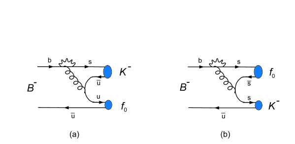
Figure 1: Penguin contributions to $B^{-}\to f_{0}(980)K^{-}$.

The decay mode $B\to f_{0}(980)K$ has been studied in Chen within the framework of the pQCD approach based on the $k_{T}$ factorization theorem. It is found that the branching ratio is of order $5\times 10^{-6}$ (see Fig. 2 of the second reference in Chen ), which is smaller than the measured value by a factor of 3.

The penguin-dominated $B\to f_{0}K$ decay receives two different types of penguin contributions as depicted in Fig. 1. In the expression of $B\to f_{0}K$ decay amplitudes given in Eq. (A), the superscript $u$ of the form factor $F_{0}^{Bf_{0}^{u}}$ reminds us that it is the $u$ quark component of $f_{0}$ involved in the form factor transition [Fig. 1(a)]. In contrast, the superscript $s$ of the decay constant $\bar{f}_{f_{0}}^{s}$ indicates that it is the strange quark content of $f_{0}$ responsible for the penguin contribution of Fig. 1(b). Note that $a_{4}$ and $a_{6}$ penguin terms contribute constructively to $\pi^{0}K^{-}$ but destructively to $f_{0}K^{-}$. Therefore, the contribution to $B\to f_{0}K$ from Fig. 1(a) will be severely suppressed. Likewise, the contribution from Fig. 1(b) is suppressed by $\bar{r}_{\chi}^{f_{0}}\sim m_{f_{0}}/m_{b}$. Hence, it is naively expected that the $f_{0}K$ rate is smaller than the $\pi^{0}K$ one. However, as shown in Appendix B, the scale dependent decay constant $\bar{f}_{f_{0}}^{s}$ is much larger than $f_{\pi}$ owing to its scale dependence and the large radiative corrections to the quark loops in the OPE series. As a consequence, the branching ratio of $B\to f_{0}K$ turns out to be comparable to and even larger than $B\to\pi^{0}K$.

Based on the QCD factorization approach, we obtain ${\cal B}(B^{-}\to f_{0}K^{-})=(9.0-13.5)\times 10^{-6}$ for $25^{\circ}<\theta<40^{\circ}$ and $(12.0-17.2)\times 10^{-6}$ for $140^{\circ}<\theta<165^{\circ}$ (Fig. 2), where only the central values are quoted. Hence, the short-distance contributions suffice to explain the observed large rates of $f_{0}K^{-}$ and $f_{0}\overline{K}^{0}$.

Figure 2: The branching ratio of $B^{-}\to f_{0}(980)K^{-}$ versus the mixing angle $\theta$ of strange and nonstrange components of $f_{0}(980)$, where the middle bold solid curve inside the allowed region corresponds to the central value. For simplicity, theoretical errors due to weak annihilation and hard spectator interactions are not taken into account. The horizontal band within the dashed lines shows the experimentally allowed region with one sigma error.

Thus far we have discussed $f_{0}K$ modes with the two-quark assignment for the $f_{0}(980)$. It is natural to ask what will happen if $f_{0}$ is a four-quark bound state. Naively, one may wonder if the energetic $f_{0}(980)$ produced in $B$ decays is dominated by the four-quark configuration as it requires to pick up two energetic quark-antiquark pairs to form a fast-moving light four-quark scalar meson. The Fock states of $f_{0}(980)$ consist of $q\bar{q}$, $q^{2}\bar{q}^{2}$, $q\bar{q}g,\cdots,$ etc. It is thus expected that the distribution amplitude of $f_{0}$ would be smaller in the four-quark model than in the two-quark picture. Naively, the observed $B\to f_{0}(980)K$ rates seem to imply that the two-quark component of $f_{0}(980)$ play an essential role for this weak decay.

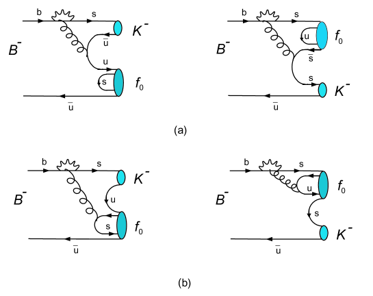
Figure 3: Penguin contributions to $B^{-}\to f_{0}(980)K^{-}$in the 4-quark picture for $f_{0}(980)$.

Nevertheless, as pointed out in Brito , the number of the quark diagrams for the penguin contributions to $B\to f_{0}(980)K$ (Fig. 3) in the four-quark scheme for $f_{0}(980)$ is two times as many as that in the usual 2-quark picture (Fig. 1). That is, besides the factorizable diagrams in Fig. 3(a), there exist two more nonfactorizable contributions depicted in Fig. 3(b). Therefore, a priori there is no reason that the $B\to f_{0}(980)K$ rate will be suppressed if $f_{0}$ is a four-quark state. However, in practice, it is difficult to give quantitative predictions based on this scenario as the nonfactorizable diagrams are usually not amenable. Moreover, even for the factorizable contributions, the calculation of the $f_{0}(980)$ decay constant and its form factors is beyond the conventional quark model, though an attempt has been made in Brito . In order to make quantitative calculations for $B\to f_{0}(980)K$, we have assumed the conventional 2-quark description of the light scalar mesons. However, as explained before, the fact that its rate can be accommodated in the 2-quark picture for $f_{0}(980)$ does not mean that the measurement of $B\to f_{0}K$ can be used to distinguish between the 2-quark and 4-quark assignment for $f_{0}(980)$.

We next turn to $B\to a_{0}(980)K$ decays. A main difference between $a_{0}^{0}K$ and $f_{0}K$ modes is that the latter receives the dominant contribution from the $s$ quark component of the $f_{0}$ [see Fig. 1(b)], while such a contribution vanishes in the former mode even when $a_{0}^{0}$ is assigned with the $s\bar{s}(u\bar{u}-d\bar{d})/\sqrt{2}$ quark content. Because of the destructive interference between the $a_{4}$ and $a_{6}$ terms, the penguin contributions related to the $u$ quark component of the $a_{0}$ and $f_{0}$ are largely suppressed. Consequently, the weak annihilation contribution becomes as important as the penguin one. For example, the branching ratio of $a_{0}^{0}K^{-}$ is of order $3.3\times 10^{-7}$ in the absence of weak annihilation, while it becomes $2.4\times 10^{-6}$ when weak annihilation is turned on. From Table 5 we see that $\Gamma(B\to a_{0}^{0}K)\ll\Gamma(B\to f_{0}K)$ and the $a_{0}^{\pm}K$ rate is enhanced by a factor of 2 for charged $a_{0}$. The predicted central value of ${\cal B}(\overline{B}^{0}\to a_{0}^{+}K^{-})$ is larger than the current upper limit by a factor of 2. However, one cannot conclude definitely at this stage that the 2-quark picture for $a_{0}(980)$ is ruled out since it is still consistent with experiment when theoretical uncertainties are taken into account. Nevertheless, as we shall see below, when the unknown parameter $\rho_{A}$ for weak annihilation is fixed to be of order 0.7 in order to accommodate the $K_{0}^{*}(1430)\pi$ data, this in turn implies too large $a_{0}(980)K$ rates compared to experiment. There will be more about this when we discuss $B\to K^{*}_{0}(1430)\pi$ decays. Note that the prediction of ${\cal B}(B^{-}\to a_{0}^{-}(980)\overline{K}^{0})=15\times 10^{-6}$ made in Minkowski in the absence of the gluonic component is ruled out by experiment.

IV.2.2 $B\to a_{0}(980)\pi,f_{0}(980)\pi$ decays

The tree dominated decays $B\to a_{0}(980)\pi,f_{0}(980)\pi$ are governed by the $B\to a_{0}$ and $B\to f_{0}^{u}$ transition form factors, respectively. The $f_{0}\pi$ rate is rather small because of the small $u\bar{u}$ component in the $f_{0}(980)$ and the destructive interference between $a_{4}$ and $a_{6}$ penguin terms. Since the $B\to a_{0}(980)$ form factor is predicted to be similar to that for $B\to\pi$ one according to the covariant light-front model (see Sec. III.C), it is interesting to compare $B\to a_{0}\pi$ decays with $B\to\pi\pi$. First, $\overline{B}^{0}\to a_{0}^{-}\pi^{+}$ is highly suppressed. This means that the $B^{0}-\overline{B}^{0}$ interference plays no role in the $a_{0}^{\pm}\pi^{\mp}$ channels. Thus the decays $\overline{B}^{0}\to a_{0}^{\pm}\pi^{\mp}$ are expected to be self-tagging; that is, the charge of the pion identifies the $B$ flavor. Second, we see from Table 5 that the branching ratio ${\cal B}(\overline{B}^{0}\to a_{0}^{+}\pi^{-})\sim 7.6\times 10^{-6}$ is slightly larger than ${\cal B}(\overline{B}^{0}\to\pi^{+}\pi^{-})=(4.5\pm 0.4)\times 10^{-6}$ HFAG and that ${\cal B}(B^{-}\to\pi^{-}\pi^{0})>{\cal B}(B^{-}\to a_{0}^{0}\pi^{-})>{\cal B}(B^{-}\to a_{0}^{-}\pi^{0})$.

Just as the $a_{0}^{+}K^{-}$ mode, the predicted branching ratio ${\cal B}(\overline{B}^{0}\to a_{0}^{\pm}(980)\pi^{\mp})=(8.2^{+0.9+2.1+2.9}_{-0.7-1.9-1.9})\times 10^{-6}$ exceeds the current experimental limit of $3.3\times 10^{-6}$ by more than a factor of 2 (cf. Table 5). If the measured rate of $a_{0}^{+}\pi^{-}$ is at the level of $(1\sim 2)\times 10^{-6}$ or even smaller, this will imply a substantially smaller $B\to a_{0}$ form factor than the $B\to\pi$ one. Hence, the four-quark explanation of the $a_{0}$ (see Fig. 4) is preferred to account for the $B\to a_{0}$ form factor suppression. We shall see later that since $a_{0}(1450)$ can be described by the $q\bar{q}$ quark model, the study of $a_{0}^{+}(1450)\pi^{-}$ relative to $a_{0}^{+}(980)\pi^{-}$ can provide a more strong test on the quark content of $a_{0}(980)$. It has been claimed in Suzuki that the positive identification of $B^{0}/\overline{B}^{0}\to a_{0}^{\pm}(980)\pi^{\mp}$ is an evidence against the four-quark assignment of $a_{0}(980)$ or else for breakdown of perturbative QCD. We disagree and we argue below that if the branching ratio of $\overline{B}^{0}\to a_{0}^{+}(1450)\pi^{-}$ is measured at the level of $3\times 10^{-6}$ and the $a_{0}^{+}(980)\pi^{-}$ rate is found to be smaller, say, of order $(1\sim 2)\times 10^{-6}$, it will be likely to imply a 2-quark nature for $a_{0}(1450)$ and a four-quark assignment for $a_{0}(980)$.

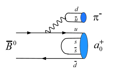
Figure 4: Tree contribution to $\overline{B}^{0}\to a_{0}^{+}(980)\pi^{-}$in the 4-quark picture for $a_{0}(980)$.

In short, although it is unlikely that the penguin-dominated decay $B\to f_{0}K$ can be used to distinguish between the 2-quark and 4-quark assignment for $f_{0}(980)$, the decays $B\to a_{0}\pi$ and $a_{0}K$ may serve for the same purpose for $a_{0}(980)$. For example, the former mode is tree dominated and its amplitude is proportional to the form factor $F_{0}^{Ba_{0}}$ which is suppressed in the four-quark model for $a_{0}(980)$. It has been claimed in Delepine that a best candidate to distinguish the nature of the $a_{0}$ scalar is ${\cal B}(B^{-}\to a_{0}^{-}\pi^{0})$ as the prediction for a four-quark model is one order of magnitude smaller than for the two quark assignment. We see from Table 5 that the branching ratio of this mode is only of order $2\times 10^{-7}$ even when $a_{0}(980)$ is treated as a 2-quark state. Experimentally, it would be extremely difficult to test the $a_{0}(980)$ nature from the study of $a_{0}^{-}(980)\pi^{0}$.

It is commonly assumed that only the valence quarks of the initial and final state hadrons participate in the decays. Nevertheless, a real hadron in QCD language should be described by a set of Fock states for which each state has the same quantum number as the hadron. For example,

$$|a^{+}(980)\rangle = \psi_{u\bar{d}}^{a_{0}}|u\bar{d}\rangle+\psi_{u\bar{d}g}^{a_{0}}|u\bar{d}g\rangle+\psi_{u\bar{d}s\bar{s}}^{a_{0}}|u\bar{d}s\bar{s}\rangle+\dots\,.$$ (56)

The possibility that $a_{0}(980)$ can be viewed as a bound state of four quarks at low energies, while its 2-quark component manifests at high energies is also allowed by current experiments.

Note that the production of $a_{0}(980)$ in hadronic $B$ decays has not been seen so far and only some limits have been set. In contrast, the $a_{0}(980)$ production in charm decays has been measured in several places, e.g. $D^{0}\to K^{0}a_{0}^{0}(980)$ and $K^{-}a_{0}^{+}(980)$ in the three-body decays $D^{0}\to K^{+}K^{-}\overline{K}^{0}$ BaBar3K . It is conceivable that the scalar resonance $a_{0}(980)$ in $B$ decays will be seen at $B$ factories soon.

IV.2.3 $B\to K_{0}^{*}(1430)\pi$ decays

For weak decays involving scalar mesons above 1 GeV such as $K_{0}^{*}(1430)$, $a_{0}(1450)$ and $f_{0}(1500)$ we consider two different scenarios to evaluate their decay constants and LCDAs based on the QCD sum rule method (see Appendices B and C): i) $K_{0}^{*}(1430),a_{0}(1450),f_{0}(1500)$ are treated as the first excited states of $\kappa,a_{0}(980)$ and $f_{0}(980)$, respectively, and (ii) they are the lowest lying resonances and the corresponding first excited states lie in between $(2.0\sim 2.3)$ GeV. Scenario 2 corresponds to the case that light scalar mesons are four-quark bound states, while all scalar mesons are made of two quarks in scenario 1. The resultant decay constants and LCDAs for the scalar mesons above 1 GeV in these two different scenarios are summarized in Appendices B and C. The $B\to K^{*}_{0}(1430)$ form factors in scenarios 1 and 2 can be found in Table 4. It should be stressed that the decay constants of $K_{0}^{*}(1430),a_{0}(1450),f_{0}(1500)$ have the signs flipped from scenario 1 to scenario 2 as explained in footnote 9 in Appendix B.

As mentioned in the Introduction, there exists a two-fold experimental ambiguity in extracting the branching ratio of $B^{-}\to\overline{K}_{0}^{*}(1430)^{0}\pi^{-}$: Belle found two different solutions for its branching ratios from the fit to $B^{+}\to K^{+}\pi^{+}\pi^{-}$ events BelleKpipi . The larger solution is consistent with BaBar BaBarKpipi while the other one is smaller by a factor of 5 [see Eq. (4)]. It appears that the larger of the two solutions, namely, ${\cal B}(B^{-}\to\overline{K}_{0}^{*}(1430)^{0}\pi^{-})\sim 45\times 10^{-6}$ , is preferable as it is consistent with the BaBar measurement and supported by a phenomenological estimate in Chernyak . However, since $B^{-}\to\overline{K}^{0}\pi^{-}$ has a branching ratio of order $24\times 10^{-6}$ HFAG , one may wonder why the $\overline{K}_{0}^{*0}\pi^{-}$ production is much more favorable than $\overline{K}^{0}\pi^{-}$, while the $\overline{K}^{*0}_{0}\pi^{0}$ mode is comparable to $\overline{K}^{0}\pi^{0}$ (see Table 2).

To proceed we consider the pure penguin decays $B^{-}\to\overline{K}^{*0}_{0}\pi^{-}$ and $B^{-}\to\overline{K}^{0}\pi^{-}$ for the purpose of illustration. The dominant penguin amplitudes read [see also Eq. (A)]

$$A(B^{-}\to\overline{K}^{*0}_{0}\pi^{-}) \propto (a_{4}^{p}-r_{\chi}^{K^{*}_{0}}a_{6}^{p})_{\pi K_{0}^{*}}\,f_{K^{*}_{0}}F_{0}^{B\pi}(m^{2}_{K^{*}_{0}})(m_{B}^{2}-m_{\pi}^{2}),$$

$$A(B^{-}\to\overline{K}^{0}\pi^{-}) \propto (a_{4}^{p}+r_{\chi}^{K}a_{6}^{p})_{\pi K}\,f_{K}F_{0}^{B\pi}(m^{2}_{K})(m_{B}^{2}-m_{\pi}^{2}),$$ (57)

where we have neglected annihilation contributions for the time being. Although the decay constant of $K^{*}_{0}(1430)$, which is $37\pm 4$ MeV in scenario 2 [cf. Eq. (97)], is much smaller than that of the kaon, it is compensated by the large ratio $r_{\chi}^{K_{0}^{*}}=8.9$ at $\mu=2.1$ GeV compared to $r_{\chi}^{K}=1.1$. Since the penguin coefficient $a_{6}$ is the same for both $K_{0}^{*}\pi$ and $K\pi$ modes, it is thus expected that $\Gamma(\overline{K}^{*0}_{0}\pi^{-})/\Gamma(\overline{K}^{0}\pi^{-})\approx 3.2$ in the absence of the $a_{4}$ contribution. When $a_{4}$ is turned on, we notice that its contribution is destructive to $\overline{K}^{*0}_{0}\pi^{-}$ and constructive to $\overline{K}^{0}\pi^{-}$. In order to see the effect of $a_{4}$ explicitly we give the numerical results for the relevant $a_{i}^{p}(\pi K_{0}^{*})$ at the scale $\mu=2.1$ GeV

$$a_{1}=1.417-i0.181,\qquad\qquad\quad~{}~{}a_{2}=0.673-i0.111,$$

$$a_{4}^{u}=-0.199-i0.009,\qquad\qquad\quad a_{4}^{c}=-0.162-i0.059,$$

$$a_{6}^{u}=-0.0558-i0.0163,\qquad\qquad a_{6}^{c}=-0.0602-i0.0039,$$

$$a_{8}^{u}=(79.4-i4.8)\times 10^{-5},\qquad\quad~{}a_{8}^{c}=(78.5-i2.4)\times 10^{-5},$$

$$a_{10}^{u}=(70-i64)\times 10^{-4},\qquad\qquad a_{10}^{c}=(70-i62)\times 10^{-4},$$ (58)

and for $a_{i}^{p}(\pi K)$

$$a_{1}=0.993+i0.0288,\qquad\qquad\quad~{}a_{2}=0.144-i0.111,$$

$$a_{4}^{u}=-0.0267-i0.0183,\qquad\qquad a_{4}^{c}=-0.0343-i0.0064,$$

$$a_{6}^{u}=-0.0568-i0.0163,\qquad\qquad a_{6}^{c}=-0.0612-i0.0039,$$

$$a_{8}^{u}=(74.4-i4.5)\times 10^{-5},\qquad\quad~{}a_{8}^{c}=(73.6-i2.3)\times 10^{-5},$$

$$a_{10}^{u}=(-208+i90)\times 10^{-5},\quad\quad~{}~{}a_{10}^{c}=(-209+i90)\times 10^{-5},$$ (59)

where scenario 2 has been used to evaluate both $a_{i}^{p}(\pi K_{0}^{*})$ and $a_{i}^{p}(\pi K)$. Comparing Eq. (IV.2.3) and with Eq. (IV.2.3), it is evident that vertex and spectator interaction corrections to $a_{1},a_{2},a_{4}$ and $a_{10}$ for $\pi K^{*}_{0}$ are quite large compared to the corresponding $a_{i}(\pi K)$ due mainly to the different nature of the $K^{*}_{0}$ LCDA. Note that the $a_{6}$ and $a_{8}$ penguin terms remain intact as they do not receive vertex and hard spectator interaction contributions. Since the magnitude of $a_{4}^{p}(\pi K_{0}^{*})$ is increased significantly, it is clear that the $\overline{K}_{0}^{*0}\pi^{-}$ rate eventually becomes slightly smaller than $\overline{K}^{0}\pi^{-}$ due to the large destructive contribution from $a_{4}^{p}(\pi K^{*}_{0})$. Hence, we conclude that ${\cal B}(B^{-}\to\overline{K}_{0}^{*0}\pi^{-})\sim 1\times 10^{-5}\sim{1\over 2}{\cal B}(B^{-}\to\overline{K}^{0}\pi^{-})$ in the absence of weak annihilation contributions.

¿From Tables 5 and 6 it is clear that when weak annihilation is turned on, the $K^{*}_{0}\pi$ rates are highly suppressed in scenario 1 due to the large destructive contributions from the defaulted weak annihilation. In order to accommodate the data, one has to take into account the power corrections due to the non-vanishing $\rho_{A}$ and $\rho_{H}$ from weak annihilation and hard spectator interactions, resepctively. Since power corrections are dominated by weak annihilation, a fit to the data yields $\rho_{A}\sim 0.4$ for scenario 2 and $\rho_{A}\sim 0.7$ for scenario 1, where we have taken $\phi_{A}\approx 0$.

We see from Eq. (A) that the amplitudes of $B^{-}\to\overline{K}^{*0}_{0}\pi^{-}$ and $\overline{B}^{0}\to K^{*-}_{0}\pi^{+}$ are identical when the small contributions from the electroweak penguin and $\lambda_{u}a_{1}$, $\lambda_{u}b_{2}$ terms are neglected. This amounts to assuming the dominance of the $\Delta I=0$ penguin contributions. Hence, these two modes should have the same rates under the isospin approximation Gronau . Likewise, $\Gamma(\overline{B}^{0}\to\overline{K}^{*0}_{0}\pi^{0})/\Gamma(\overline{B}^{0}\to K^{*-}_{0}\pi^{+})=1/2$ is expected to hold in the isospin limit. Indeed, it is found in QCD factorization calculations that

$$R_{1}\equiv{{\cal B}(\overline{B}^{0}\to\overline{K}_{0}^{*0}(1430)\pi^{0})\over{\cal B}(\overline{B}^{0}\to K_{0}^{*-}(1430)\pi^{+})} = \cases{0.51^{+0.01+0.08+0.04}_{-0.02-0.02-0.06}&scenario~{}1;\cr 0.47^{+0.01+0.02+0.04}_{-0.02-0.01-0.10}&scenario~{}2;}$$

$$R_{2}\equiv{{\cal B}(B^{-}\to K_{0}^{*-}(1430)\pi^{0})\over{\cal B}(B^{-}\to\overline{K}_{0}^{*0}(1430)\pi^{-})} = \cases{0.30^{+0.03+0.43+0.79}_{-0.02-0.02-0.02}&scenario~{}1;\cr 0.58^{+0.05+0.01+0.17}_{-0.03-0.01-0.05}&scenario~{}2;}$$ (60)

$$R_{3}\equiv{\tau(B^{0}){\cal B}(B^{-}\to\overline{K}_{0}^{*0}(1430)\pi^{-})\over\tau(B^{-}){\cal B}(\overline{B}^{0}\to K_{0}^{*-}(1430)\pi^{+})} = \cases{0.81^{+0.06+0.62+0.93}_{-0.07-0.04-0.57}&scenario~{}1;\cr 0.90^{+0.05+0.03+0.18}_{-0.06-0.03-0.27}&scenario~{}2.}$$

Consequently, the ambiguity in regard to $B^{-}\to\overline{K}_{0}^{*0}\pi^{-}$ found by Belle can be resolved by the measurement of $\overline{B}^{0}\to K^{*-}_{0}\pi^{+}$. As noted in passing, both BaBar and Belle measurements of $B^{-}\to\overline{K}^{*0}_{0}\pi^{-}$ and $B^{0}\to K^{*-}_{0}\pi^{+}$ [see Eq. (4) and Table 2] do respect the isospin relation. It is also important to measure the ratio of ${\cal B}(\overline{B}^{0}\to\overline{K}_{0}^{*0}(1430)\pi^{0})/{\cal B}(\overline{B}^{0}\to K_{0}^{*-}(1430)\pi^{+})$ to see if it is close to one half. At any rate, both BaBar and Belle should measure all $K^{*}_{0}(1430)\pi$ modes with a careful Dalitz plot analysis of nonresonant contributions to three-body decays to avoid any possible ambiguities.

We now turn to the implications of sizable weak annihilation characterized by the parameter $\rho_{A}$ which is of order 0.7 in scenario 1 and ${\cal O}(0.4)$ in scenario 2. We find that all the calculated $a_{0}(980)K$ rates are too large compared to experiment. For example, ${\cal B}(\overline{B}^{0}\to a_{0}^{+}(980)K^{-})\approx 31.4\times 10^{-6}$ for $\rho_{A}=0.7$ and $\approx 14.6\times 10^{-6}$ for $\rho_{A}=0.4$. Both are ruled out by the current limit of $1.9\times 10^{-6}$. This clearly indicates that $a_{0}(980)$ cannot be a purely two-quark state and that scenario 2 in which the light scalar meson is assigned to be a four-quark state is preferable.

IV.2.4 $B\to a_{0}(1450)K,a_{0}(1450)\pi$ decays

For $\overline{B}\to a_{0}(1450)\pi$ and $a_{0}(1450)K$ decays, the calculated results should be reliable as the $a_{0}(1450)$ can be described by the $q\bar{q}$ quark model. Just as $a_{0}(980)K$ modes, weak annihilation gives a dominant contribution to $a_{0}(1450)K$ rates. It is found that their rates are much larger in scenario 1 than in scenario 2 due to the relative sign difference between the Gegenbauer moments $B_{1}$ and $B_{3}$ for $a_{0}(1450)$ and the sign of the $a_{0}(1450)$ decay constant flipped in these two scenarios (see Tables 10 and 11). The interference pattern between the penguin and annihilation amplitudes is generally opposite in scenarios 1 and 2. For example, the interference in $\overline{B}^{0}\to a_{0}^{+}(1450)K^{-}$ is constructive in scenario 1 but becomes destructive in scenario 2. By the same token, the $a_{0}^{+}(1450)\pi^{-}$ and $a_{0}^{0}(1450)\pi^{0}$ rates are also quite different in scenarios 1 and 2.

As discussed in the previous subsection on $K_{0}^{*}(1430)\pi$, predictions under scenario 2 are more preferable. Hence, if the branching ratio of $\overline{B}^{0}\to a_{0}^{\pm}(1450)\pi^{\mp}$ is measured at the level of $4\times 10^{-6}$ and the $a_{0}^{+}(980)\pi^{-}$ rate is found to be smaller, say, of order $(1\sim 2)\times 10^{-6}$ or even smaller than this, it will be likely to imply a 2-quark nature for $a_{0}(1450)$ and a four-quark assignment for $a_{0}(980)$. Note that the naive estimate of $20\times 10^{-6}$ made by Chernyak for this mode appears to be too large due to the usage of a large $B\to a_{0}(1450)$ form factor, $F_{0}^{Ba_{0}(1450)}(0)=0.46$. Experimentally, $a_{0}(1450)$ will be more difficult to identify than $a_{0}(980)$ because of its broad width, $265\pm 13$ MeV PDG .

IV.2.5 $\overline{B}^{0}\to\kappa^{+}K^{-}$ as spectroscope for $\kappa$ four quark state

As for $\kappa$ (or $K_{0}^{*}(800)$), there is a nice and unique place where one can discriminate between the 4-quark and 2-quark pictures for the $\kappa$ meson, namely, the $\overline{B}^{0}\to\kappa^{+}K^{-}$ decay. Recall that $\overline{B}^{0}\to K^{+}K^{-}$ is strongly suppressed as it can only proceed through the $W$-exchange diagram. The experimental upper bound on its branching ratio is $0.6\times 10^{-6}$ HFAG ; PDG while it is predicted to be of order $1\times 10^{-8}$ theoretically (see e.g. BN ). Naively $\overline{B}^{0}\to\kappa^{+}K^{-}$ is also rather suppressed if $\kappa$ is made of two quarks. However, if $\kappa$ has primarily a four-quark content, this decay can receive a tree contribution as depicted in Fig. 5(b). Hence, if $\overline{B}^{0}\to\kappa^{+}K^{-}$ is observed at the level of ${\ \lower-1.2pt\vbox{\hbox{\hbox to0.0pt{$>$\hss}\lower 5.0pt\vbox{\hbox{$\sim$} }}}\ }10^{-7}$, it may imply a four-quark content for the $\kappa$. Presumably, this can be checked from the Dalitz plot analysis of the three-body decay $\overline{B}^{0}\to K^{+}K^{-}\pi^{0}$ or $\overline{B}^{0}\to K^{0}K^{-}\pi^{+}$. As noticed before, scenario 2 is more favored for explaining the $B\to K^{*}_{0}(1430)\pi$ data. This already implies that $\kappa$ is preferred to be a four-quark state.

Unlike the other light scalar mesons, the experimental evidence for $\kappa$ is still controversial. The $\kappa$ state has been reported by E791 in the analysis of $D^{+}\to K^{-}\pi^{+}\pi^{+}$ with the mass $797\pm 19\pm 43$ MeV and width $410\pm 43\pm 87$ MeV E791 . However, CLEO did not see evidence for the $\kappa$ in $D^{0}\to K^{-}\pi^{+}\pi^{0}$ CLEOkappa . The $\kappa$ state was also reported by the reanalyses of LASS data on $\pi K$ scattering phase shifts using the $T$-matrix method Bugg and the unitarization method combined with chiral symmetry Zheng . Most recently, BES has reported the evidence for the $\kappa$ in $J/\psi\to\overline{K}^{*0}K^{+}\pi^{-}$ process with the mass $878\pm 23^{+64}_{-55}$ MeV and width $499\pm 52^{+55}_{-87}$ MeV BESII .

It is interesting to notice that the decays $\overline{B}^{0}\to D_{s}^{+}K^{-}$ and $\overline{B}^{0}\to D_{s0}^{*}(2317)^{+}K^{-}$, the analogues of $\overline{B}^{0}\to K^{+}K^{-}$ and $\overline{B}^{0}\to\kappa^{+}K^{-}$, have been measured recently. The measured branching ratios are ${\cal B}(\overline{B}^{0}\to D_{s}^{+}K^{-})=(3.8\pm 1.3)\times 10^{-5}$ PDG and ${\cal B}(\overline{B}^{0}\to D_{s0}^{*+}K^{-}){\cal B}(D_{s0}^{*+}\to D_{s}^{+}\pi^{0})=(5.3^{+1.5}_{-1.3}\pm 1.6)\times 10^{-6}$ BelleDs0K . Since $D_{s0}^{*}(2317)^{+}$ is dominated by the hadronic decay into $D_{s}^{+}\pi^{0}$, it is clear that $\Gamma(\overline{B}^{0}\to D_{s0}^{*+}K^{-}){\ \lower-1.2pt\vbox{\hbox{\hbox to0.0pt{$>$\hss}\lower 5.0pt\vbox{\hbox{$\sim$} }}}\ }\Gamma(\overline{B}^{0}\to D_{s}^{+}K^{-})$. These two decays can only proceed via a short-distance $W$-exchange process or through the long-distance final-state rescattering processes $\overline{B}^{0}\to D^{+}\pi^{-}\to D_{s}^{+}K^{-}$ and $\overline{B}^{0}\to D^{*+}_{0}\pi^{-}\to D^{*+}_{s0}K^{-}$. (In fact, the rescattering process has the same topology as $W$-exchange.) Since ${\cal B}(\overline{B}^{0}\to D^{+}\pi^{-})\approx 2.8\times 10^{-3}\gg{\cal B}(\overline{B}^{0}\to D_{s}^{+}K^{-})$, it is thus expected that the decay $\overline{B}^{0}\to D_{s}^{+}K^{-}$ is dominated by the long-distance rescattering process. As ${\cal B}(\overline{B}^{0}\to D_{0}^{*+}\pi^{-})<1.8\times 10^{-4}$ PDG , we will naively conclude that $\Gamma(\overline{B}^{0}\to D_{s0}^{*+}K^{-})/\Gamma(\overline{B}^{0}\to D_{s}^{+}K^{-})<0.06$, in contradiction to the experimental observation. Nevertheless, if $D_{s0}^{*}(2317)^{+}$ is a bound state of $c\bar{s}d\bar{d}$ CH , then a tree diagram similar to Fig. 5(b) will contribute and this may allow us to explain why $\Gamma(\overline{B}^{0}\to D_{s0}^{*+}K^{-}){\ \lower-1.2pt\vbox{\hbox{\hbox to0.0pt{$>$\hss}\lower 5.0pt\vbox{\hbox{$\sim$} }}}\ }\Gamma(\overline{B}^{0}\to D_{s}^{+}K^{-})$.

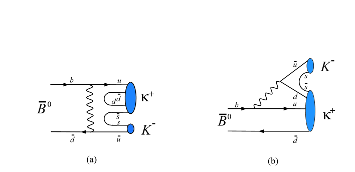
Figure 5: Annihilation and tree contributions to $\overline{B}^{0}\to\kappa^{+}K^{-}$ in the 4-quark picture for $\kappa$.

IV.2.6 $B\to\sigma\pi$ decays

The tree dominated $B\to\sigma\pi$ decays are expected to have similar rates as $B\to\pi^{0}\pi$ ones if the $\sigma$ meson is assumed to be a bound state of 2 quarks. Assuming that $\sigma$ has similar decay constant and LCDA as $f_{0}(980)$, it is found that ${\cal B}(B^{-}\to\sigma\pi^{-})\approx 4.5\times 10^{-6}$ and ${\cal B}(\overline{B}^{0}\to\sigma\pi^{0})\approx 1.7\times 10^{-7}$. The former is to be compared with the upper limit $4.1\times 10^{-6}$ BaBar3pi .

Table 7: Same as Table 5 except for CP asymmetries (in %).

Mode	Theory	Expt	Mode	Theory	Expt
$B^{-}\to f_{0}(980)K^{-}$	$0.4^{+0.0+0.0+0.6}_{-0.0-0.0-0.6}$	$-2.0^{+6.8}_{-6.5}$	$\overline{B}^{0}\to f_{0}(980)\overline{K}^{0}$	$0.7^{+0.0+0.0+0.1}_{-0.0-0.0-0.1}$	$-6\pm 21$
$B^{-}\to f_{0}(980)\pi^{-}$	$-2.0^{+0.2+0.1+43.0}_{-0.2-3.4-41.9}$	$-50\pm 54$	$\overline{B}^{0}\to f_{0}(980)\pi^{0}$	$38.6^{+11.8+~{}2.9+~{}44.1}_{-11.0-18.3-114.4}$
$B^{-}\to a_{0}^{0}(980)K^{-}$	$3.8^{+1.6+1.5+52.8}_{-1.1-1.5-63.6}$		$\overline{B}^{0}\to a_{0}^{+}(980)K^{-}$	$3.4^{+1.4+1.4+51.3}_{-1.0-1.4-61.9}$
$B^{-}\to a_{0}^{-}(980)\overline{K}^{0}$	$0.9^{+0.1+0.1+1.2}_{-0.1-0.2-0.9}$		$\overline{B}^{0}\to a_{0}^{0}(980)\overline{K}^{0}$	$0.7^{+0.1+0.1+1.0}_{-0.1-0.1-0.5}$
$B^{-}\to a_{0}^{0}(980)\pi^{-}$	$-0.6^{+0.1+0.1+3.6}_{-0.1-0.2-3.8}$		$\overline{B}^{0}\to a_{0}^{+}(980)\pi^{-}$	$-0.3^{+0.2+0.5+23.6}_{-0.2-0.3-22.8}$
$B^{-}\to a_{0}^{-}(980)\pi^{0}$	$-65.9^{+6.1+7.8+24.6}_{-8.3-5.2-22.0}$		$\overline{B}^{0}\to a_{0}^{-}(980)\pi^{+}$	$76.5^{+~{}5.9+4.0+21.0}_{-10.5-5.9-36.1}$
			$\overline{B}^{0}\to a_{0}^{0}(980)\pi^{0}$	$34.3^{+12.3+~{}9.1+28.6}_{-~{}8.3-11.6-30.5}$
$B^{-}\to a_{0}^{0}(1450)K^{-}$	$0.9^{+0.5+0.9+21.4}_{-0.3-0.6-18.7}$		$\overline{B}^{0}\to a_{0}^{+}(1450)K^{-}$	$0.9^{+0.5+0.9+19.7}_{-0.3-0.6-18.9}$
$B^{-}\to a_{0}^{-}(1450)\overline{K}^{0}$	$0.3^{+0.1+0.1+0.2}_{-0.1-0.1-6.6}$		$\overline{B}^{0}\to a_{0}^{0}(1450)\overline{K}^{0}$	$0.3^{+0.1+0.1+0.2}_{-0.0-0.1-1.7}$
$B^{-}\to a_{0}^{0}(1450)\pi^{-}$	$-2.9^{+0.2+0.4+5.4}_{-0.2-0.3-5.7}$		$\overline{B}^{0}\to a_{0}^{+}(1450)\pi^{-}$	$0.4^{+0.1+0.5+36.2}_{-0.1-0.3-35.4}$
$B^{-}\to a_{0}^{-}(1450)\pi^{0}$	$19.8^{+1.8+3.2+44.9}_{-6.4-3.6-46.6}$		$\overline{B}^{0}\to a_{0}^{-}(1450)\pi^{+}$	$59.2^{+13.8+12.6+~{}33.0}_{-36.7-66.6-152.7}$
			$\overline{B}^{0}\to a_{0}^{0}(1450)\pi^{0}$	$-32.8^{+11.7+7.8+66.2}_{-16.7-6.6-52.4}$
$B^{-}\to\overline{K}^{*0}_{0}(1430)\pi^{-}$	$-4.4^{+2.8+~{}4.1+63.8}_{-4.9-25.7-30.5}$	$-5^{+5}_{-8}$	$\overline{B}^{0}\to K^{*-}_{0}(1430)\pi^{+}$	$15.1^{+5.0+18.5+16.1}_{-3.6-~{}5.9-21.2}$	$-7\pm 14$
$B^{-}\to K^{*-}_{0}(1430)\pi^{0}$	$-42.1^{+12.6+78.6+128.7}_{-10.1-~{}2.1-~{}12.3}$		$\overline{B}^{0}\to\overline{K}^{*0}_{0}(1430)\pi^{0}$	$3.4^{+0.4+0.3+10.8}_{-0.3-7.4-~{}9.1}$	$-34\pm 19$

Table 8: Same as Table 6 except for CP asymmetries (in %).

Mode	Theory	Expt	Mode	Theory	Expt
$B^{-}\to a_{0}^{0}(1450)K^{-}$	$54.7^{+~{}2.3+~{}3.6+~{}10.4}_{-33.1-16.2-101.0}$		$\overline{B}^{0}\to a_{0}^{+}(1450)K^{-}$	$53.3^{+~{}4.8+~{}5.3+10.0}_{-35.0-18.3-96.4}$
$B^{-}\to a_{0}^{-}(1450)\overline{K}^{0}$	$19.9^{+~{}4.1+~{}8.8+8.4}_{-17.0-13.5-4.5}$		$\overline{B}^{0}\to a_{0}^{0}(1450)\overline{K}^{0}$	$4.9^{+0.6+0.5+1.9}_{-6.5-6.2-6.2}$
$B^{-}\to a_{0}^{0}(1450)\pi^{-}$	$-0.9^{+0.2+0.1+6.3}_{-0.2-0.3-6.6}$		$\overline{B}^{0}\to a_{0}^{+}(1450)\pi^{-}$	$-0.7^{+0.0+0.3+46.9}_{-0.0-0.2-45.2}$
$B^{-}\to a_{0}^{-}(1450)\pi^{0}$	$-41.4^{+6.7+1.0+123.7}_{-6.2-1.7-~{}64.8}$		$\overline{B}^{0}\to a_{0}^{-}(1450)\pi^{+}$	$37.6^{+10.0+1.3+48.6}_{-11.9-2.1+68.0}$
			$\overline{B}^{0}\to a_{0}^{0}(1450)\pi^{0}$	$20.8^{+7.5+3.3+43.3}_{-4.9-4.0-45.6}$
$B^{-}\to\overline{K}^{*0}_{0}(1430)\pi^{-}$	$1.1^{+1.3+0.2+~{}8.0}_{-0.7-0.1-17.8}$	$-5^{+5}_{-8}$	$\overline{B}^{0}\to K^{*-}_{0}(1430)\pi^{+}$	$-3.8^{+1.9+0.3+~{}8.3}_{-3.6-0.3-13.2}$	$-7\pm 14$
$B^{-}\to K^{*-}_{0}(1430)\pi^{0}$	$4.2^{+3.6+1.2+5.0}_{-2.9-1.2-3.7}$		$\overline{B}^{0}\to\overline{K}^{*0}_{0}(1430)\pi^{0}$	$0.6^{+0.5+0.1+0.7}_{-0.3-0.1-0.7}$	$-34\pm 19$

Table 9: Mixing-induced CP parameter $\Delta S\equiv\sin 2\beta_{\rm eff}-\sin 2\beta_{\rm CKM}$ in scenarios 1 and 2 as explained in Appendices B and C. The sources of theoretical errors are same as in previous tables except the last one is from the uncertainty in the unitarity angle $\gamma$.

Mode	Theory (Scenario 1)	Theory (Scenario 2)
$\overline{B}{}^{0}\to f_{0}^{0}(980)K_{S}$	$0.023^{+0.000+0.000+0.001+0.001}_{-0.000-0.000-0.001-0.001}$
$\overline{B}{}^{0}\to a_{0}^{0}(980)K_{S}$	$0.022^{+0.000+0.000+0.005+0.001}_{-0.000-0.000-0.006-0.001}$
$\overline{B}{}^{0}\to a_{0}^{0}(1450)K_{S}$	$0.023^{+0.000+0.000+0.027+0.001}_{-0.000-0.000-0.001-0.001}$	$0.021^{+0.014+0.008+0.031+0.001}_{-0.000-0.000-0.009-0.001}$
$\overline{B}{}^{0}\to\overline{K}^{*0}_{0}(1430)\pi^{0}$	$0.004^{+0.005+0.010+0.030+0.000}_{-0.008-0.040-0.036-0.000}$	$0.021^{+0.001+0.000+0.004+0.001}_{-0.002-0.013-0.008-0.001}$

IV.2.7 Direct CP asymmetries

We see from Tables 7 and 8 that CP partial rate asymmetries in those charmless $B\to SP$ decays with branching ratios ${\ \lower-1.2pt\vbox{\hbox{\hbox to0.0pt{$>$\hss}\lower 5.0pt\vbox{\hbox{$\sim$} }}}\ }10^{-6}$ are in general at most a few percents. This is ascribed to the fact that the strong phases calculable in QCD factorization are generally small and that the observation of direct CP violation requires at least two different contributing amplitudes with distinct strong and weak phases. Hence, if the observed direct CP asymmetry is of order ${\cal O}(0.1)$ or larger, then strong phases induced from power corrections could be important. As pointed out in CCS , final-state rescattering processes can have important effects on the decay rates and their direct CP violation, especially for color-suppressed and penguin-dominated modes. However, this is beyond the scope of the present work.

IV.2.8 Mixing-induced CP asymmetries

It is of great interest to measure the mixing-induced indirect CP asymmetries $S_{f}$ for penguin-dominated modes and compare them to the one inferred from the charmonium mode ($J/\psi K_{S}$) in $B$ decays. It is expected in the Standard Model that $\sin 2\beta_{\rm eff}$ defined via $S_{f}\equiv-\eta_{f}\sin 2\beta_{\rm eff}$ with $\eta_{f}$ being the CP eigenvalue of the final state $f$ should be equal to $S_{J/\psi K_{S}}$ with a small deviation at most ${\cal O}(0.1)$ LS . See sin2beta for recent studies of $\sin 2\beta_{\rm eff}$ in some of $B\to PP$ and $PV$ modes using the QCD factorization approach with or without the presence of final state interactions. In Table 9 we show the predictions on the mixing-induced CP parameter $\Delta S\equiv\sin 2\beta_{\rm eff}-\sin 2\beta_{\rm CKM}$ for the CP eigenstates $f_{0}(980)K_{S}$, $a^{0}_{0}(980)K_{S}$, $a^{0}_{0}(1450)K_{S}$ and $\overline{K}^{*0}_{0}(1430)\pi^{0}$, where only the CP component of $\overline{K}^{*0}_{0}(1430)$ namely, $K_{S}\pi^{0}$, is considered in the last mode. In addition to the theoretical errors considered before, the uncertainty of $7^{\circ}$ in the unitarity angle $\gamma$ is included. Note that main errors arise from the uncertainties in annihilation contributions and $\gamma$. Our results indicate that $\Delta S_{f}$ in these penguin dominated modes are positive and very small.

V Conclusions

In this work we have studied the hadronic $B$ decays into a scalar meson and a pseudoscalar meson within the framework of QCD factorization. Vertex corrections, hard spectator interactions and weak annihilation contributions to the hadronic $B\to SP$ decays are studied using the QCD factorization approach. Our main results are as follows:

• Based on the QCD sum rule method, we have derived the leading-twist light-cone distribution amplitudes (LCDAs) of scalar mesons and their decay constants. It is found that the scalar decay constant is much larger than the previous estimates owing to its scale dependence and the large radiative corrections to the quark loops in the OPE series. Unlike the pseudoscalar or vector mesons, the scalar LCDAs are governed by the odd Gegenbauer polynomials.

• While it is widely believed that light scalar mesons such as $f_{0}(980)$, $a_{0}(980)$, $\kappa$ are predominately four-quark states, in practice it is difficult to make quantitative predictions on $B\to SP$ based on the four-quark picture for $S$ as it involves not only the form factors and decay constants that are beyond the conventional quark model but also additional nonfactorizable contributions that are difficult to estimate. Hence, in practice we shall assume the two-quark scenario for light scalar mesons in calculations.

• The short-distance approach suffices to explain the observed large rates of $f_{0}K^{-}$ and $f_{0}\overline{K}^{0}$ that receive major penguin contributions from the penguin process $b\to ss\bar{s}$ and are governed by the large $f_{0}$ scalar decay constant. When $f_{0}(980)$ is assigned as a four-quark bound state, there exist two times more diagrams contributing to $B\to f_{0}(980)K$. Therefore, although the $f_{0}(980)K$ rates can be accommodated in the 2-quark picture for $f_{0}(980)$, it does not mean that the measurement of $B\to f_{0}K$ can be used to distinguish between the 2-quark and 4-quark assignment for $f_{0}(980)$.

• When $a_{0}(980)$ is treated as a $q\bar{q}$ bound state, it is found that the predicted $\overline{B}^{0}\to a_{0}^{+}(980)\pi^{-}$ and $a_{0}^{+}(980)K^{-}$ rates exceed substantially the current experimental limits. Hence, a four-quark assignment for $a_{0}(980)$ is favored. The $a_{0}(980)K$ and $a_{0}(1450)K$ receive dominant contributions from weak annihilation.

• Belle found two different solutions for the branching ratios of $B^{+}\to K_{0}^{*}(1430)^{0}\pi^{+}$ from the fit to $B^{+}\to K^{+}\pi^{+}\pi^{-}$ events. The larger solution is consistent with BaBar while the other one is smaller by a factor of 5. Based on the isospin argument, we have shown that the smaller of the two solutions is ruled out by the measurements of $K_{0}^{*}(1430)^{-}\pi^{+}$ by BaBar and Belle.

• For $B\to a_{0}(1450)\pi,~{}a_{0}(1450)K$ and $K^{*}_{0}(1430)\pi$ decays, we have explored two possible scenarios for the scalar mesons above 1 GeV in the QCD sum rule method, depending on whether the light scalars $\kappa,~{}a_{0}(980)$ and $f_{0}(980)$ are treated as the lowest lying $q\bar{q}$ states or four-quark particles. We pointed out that in both scenarios, one needs sizable weak annihilation in order to accommodate the $K^{*}_{0}\pi$ data. This in turn implies that all the predicted $a_{0}(980)K$ rates in scenario 1 will be too large compared to the current limits if $a_{0}(980)$ is a bound state of two quarks. This means that the scenario in which the scalar mesons above 1 GeV are lowest lying $q\bar{q}$ scalar state and the light scalar mesons are four-quark states is preferable. The branching ratio of $\overline{B}^{0}\to a_{0}^{\pm}(1450)\pi^{\mp}$ is predicted to be at the level of $4\times 10^{-6}$.

• The decay $\overline{B}^{0}\to\kappa^{+}K^{-}$ can be used to discriminate between the 4-quark and 2-quark nature for the $\kappa$ meson. This mode is strongly suppressed if $\kappa$ is made of two quarks as it can proceed through the $W$-exchange process. However, if $\kappa$ is predominately a four-quark state, it will receive a color-allowed tree contribution. Hence, an observation of this channel at the level of ${\ \lower-1.2pt\vbox{\hbox{\hbox to0.0pt{$>$\hss}\lower 5.0pt\vbox{\hbox{$\sim$} }}}\ }10^{-7}$ would mostly imply a four-quark picture for the $\kappa$. Presumably, this can be checked from the Dalitz plot analysis of three-body decay $\overline{B}^{0}\to K^{+}K^{-}\pi^{0}$ or $\overline{B}^{0}\to K^{0}K^{-}\pi^{+}$.

• Direct $CP$ asymmetries in those decay modes with branching ratios ${\ \lower-1.2pt\vbox{\hbox{\hbox to0.0pt{$>$\hss}\lower 5.0pt\vbox{\hbox{$\sim$} }}}\ }10^{-6}$ are usually small of order a few percents. However, final-state rescattering processes can have important impact on the decay rates and their direct CP violation.

• Mixing-induced CP asymmetries in the penguin dominated $SP$ modes such as $f_{0}(980)K_{S}$, $a^{0}_{0}(980)K_{S}$, $a^{0}_{0}(1450)K_{S}$ and $\overline{K}^{*0}_{0}(1430)[K_{S}\pi^{0}]\pi^{0}$ are studied. Their deviations from $\sin 2\beta_{\rm CKM}$ are found to be positive ($\Delta S>0$) and tiny.

Appendix A Decay amplitudes of $B\to SP$

The $B\to SP$ ($PS$) decay amplitudes can be either evaluated directly or obtained readily from $B\to VP$ ($PV$) amplitudes with the replacements: $f_{V}\Phi_{V}(x)\to\Phi_{S}(x)$ and $m_{V}f_{V}^{\bot}\Phi_{v}(x)\to-m_{S}\Phi_{S}^{s}(x)$. (The factor of $i$ will be taken care of by the factorizable amplitudes of $B\to SP$ shown below.) To make the replacements more transparent, it is convenient to employ the LCDA $\Phi_{S}(x)$ in the form (28) and factor out the decay constants $f_{S}$ in $\Phi_{S}(x)$ and $\bar{f}_{S}$ in $\Phi_{S}^{s}(x)$ [see Eq. (30)], so that we have

$$\quad\Phi_{V}(x)\to\Phi_{S}(x),\qquad\Phi_{v}(x)\to\Phi_{S}^{s}(x),\qquad f_{V}\to f_{S},\qquad r^{V}_{\chi}\to-r_{\chi}^{S},$$ (61)

where

$$r_{\chi}^{V}(\mu)={2m_{V}\over m_{b}(\mu)}\,{f_{V}^{\bot}(\mu)\over f_{V}},\qquad\quad r_{\chi}^{S}(\mu)={2m_{S}\over m_{b}(\mu)}\,{\bar{f}_{S}(\mu)\over f_{S}}={2m_{S}^{2}\over m_{b}(\mu)(m_{2}(\mu)-m_{1}(\mu))},$$ (62)

and use of Eq. (15) has been made. For the neutral scalars $\sigma$, $f_{0}$ and $a_{0}^{0}$, $r_{\chi}^{S}$ becomes divergent while $f_{S}$ vanishes. In this case one needs to express $f_{S}r_{\chi}^{S}$ by $\bar{f}_{S}\bar{r}_{\chi}^{S}$ with

$$\bar{r}_{\chi}^{S}(\mu)={2m_{S}\over m_{b}(\mu)}.$$ (63)

With the above-mentioned replacements, the quantity $A_{M_{1}M_{2}}$ and the coefficients of the flavor operators $\alpha_{i}^{p}$ defined in BN read

$$A_{M_{1}M_{2}} = {G_{F}\over\sqrt{2}}\cases{(m_{B}^{2}-m_{P}^{2})F_{0}^{BP}(m_{S}^{2})f_{S};&for~{}$M_{1}M_{2}=PS$,\cr-(m_{B}^{2}-m_{S}^{2})F_{0}^{BS}(m_{P}^{2})f_{P};&for~{}$M_{1}M_{2}=SP$,}$$

$$\alpha_{3}^{p}(M_{1}M_{2}) = \cases{a_{3}^{p}(M_{1}M_{2})+a_{5}^{p}(M_{1}M_{2});&for ~{}$M_{1}M_{2}=PS$,\cr a_{3}^{p}(M_{1}M_{2})-a_{5}^{p}(M_{1}M_{2});&for ~{}$M_{1}M_{2}=SP$,}$$

$$\alpha_{4}^{p}(M_{1}M_{2}) = \cases{a_{4}^{p}(M_{1}M_{2})-r_{\chi}^{S}a_{6}^{p}(M_{1}M_{2});&for ~{}$M_{1}M_{2}=PS$,\cr a_{4}^{p}(M_{1}M_{2})-r_{\chi}^{P}a_{6}^{p}(M_{1}M_{2});&for ~{}$M_{1}M_{2}=SP$,}$$ (64)

$$\alpha_{\rm 3,EW}^{p}(M_{1}M_{2}) = \cases{a_{9}^{p}(M_{1}M_{2})+a_{7}^{p}(M_{1}M_{2});&for ~{}$M_{1}M_{2}=PS$,\cr a_{9}^{p}(M_{1}M_{2})-a_{7}^{p}(M_{1}M_{2});&for ~{}$M_{1}M_{2}=SP$,}$$

$$\alpha_{\rm 4,EW}^{p}(M_{1}M_{2}) = \cases{a_{10}^{p}(M_{1}M_{2})-r_{\chi}^{S}a_{8}^{p}(M_{1}M_{2});&for ~{}$M_{1}M_{2}=PS$,\cr a_{10}^{p}(M_{1}M_{2})-r_{\chi}^{P}a_{8}^{p}(M_{1}M_{2});&for ~{}$M_{1}M_{2}=SP$,}$$

where

$$r_{\chi}^{P}={2m_{P}^{2}\over m_{b}(\mu)(m_{2}+m_{1})(\mu)}.$$ (65)

It should be stressed that the $a_{i}^{p}F_{0}^{BP}$ and $a_{i}^{p}F_{0}^{BS}$ terms in the decay amplitudes have an opposite sign.

Applying the replacement (61) and Eq. (A) to the $B\to VP$ and $PV$ amplitudes given in Appendix of BN , we obtain the following the factorizable amplitudes of the decays $B\to f_{0}K,~{}a_{0}\pi,~{}\sigma\pi,~{}a_{0}K,~{}K_{0}^{*}\pi$

$$A(B^{-}\to f_{0}K^{-}) = -\frac{G_{F}}{\sqrt{2}}\sum_{p=u,c}\lambda_{p}^{(s)}\Bigg{\{}\left(a_{1}\delta^{p}_{u}+a_{4}^{p}-r_{\chi}^{K}a_{6}^{p}+a_{10}^{p}-r_{\chi}^{K}a_{8}^{p}\right)_{f_{0}^{u}K}$$

$$\times f_{K}F_{0}^{Bf_{0}^{u}}(m_{K}^{2})(m_{B}^{2}-m_{f_{0}}^{2})+\left(a_{6}^{p}-{1\over 2}a_{8}^{p}\right)_{Kf_{0}^{s}}\bar{r}_{\chi}^{f_{0}}\bar{f}^{s}_{f_{0}}\,F_{0}^{BK}(m^{2}_{f_{0}})(m_{B}^{2}-m_{K}^{2})$$

$$- f_{B}\bigg{[}\big{(}b_{2}\delta_{u}^{p}+b_{3}+b_{\rm 3,EW}\big{)}_{f_{0}^{u}K}+\big{(}b_{2}\delta_{u}^{p}+b_{3}+b_{\rm 3,EW}\big{)}_{Kf_{0}^{s}}\bigg{]}\Bigg{\}},$$

$$A(\overline{B}^{0}\to f_{0}\overline{K}^{0}) = -\frac{G_{F}}{\sqrt{2}}\sum_{p=u,c}\lambda_{p}^{(s)}\Bigg{\{}\left(a_{4}^{p}-r_{\chi}^{K}a_{6}^{p}-{1\over 2}(a_{10}^{p}-r_{\chi}^{K}a_{8}^{p})\right)_{f_{0}^{d}K}$$

$$\times f_{K}F_{0}^{Bf_{0}^{u}}(m_{K}^{2})(m_{B}^{2}-m_{f_{0}}^{2})+\left(a_{6}^{p}-{1\over 2}a_{8}^{p}\right)_{Kf_{0}^{s}}\bar{r}_{\chi}^{f_{0}}\bar{f}^{s}_{f_{0}}\,F_{0}^{BK}(m^{2}_{f_{0}})(m_{B}^{2}-m_{K}^{2})$$

$$- f_{B}\bigg{[}\big{(}b_{3}-{1\over 2}b_{\rm 3,EW}\big{)}_{f_{0}^{d}K}+\big{(}b_{3}-{1\over 2}b_{\rm 3,EW}\big{)}_{Kf_{0}^{s}}\bigg{]}\Bigg{\}},$$

$$A(B^{-}\to a_{0}^{0}K^{-}) = -\frac{G_{F}}{{2}}\sum_{p=u,c}\lambda_{p}^{(s)}\Bigg{\{}\left(a_{1}\delta^{p}_{u}+a_{4}^{p}-r_{\chi}^{K}a_{6}^{p}+a_{10}^{p}-r_{\chi}^{K}a_{8}^{p}\right)_{a_{0}K}$$

$$\times f_{K}F_{0}^{Ba_{0}}(m_{K}^{2})(m_{B}^{2}-m_{a_{0}}^{2})-f_{B}\big{(}b_{2}\delta_{u}^{p}+b_{3}+b_{\rm 3,EW}\big{)}_{a_{0}K}\Bigg{\}},$$

$$A(B^{-}\to a_{0}^{-}\overline{K}^{0}) = -\frac{G_{F}}{\sqrt{2}}\sum_{p=u,c}\lambda_{p}^{(s)}\Bigg{\{}\left(a_{4}^{p}-r_{\chi}^{K}a_{6}^{p}-{1\over 2}(a_{10}^{p}-r_{\chi}^{K}a_{8}^{p})\right)_{a_{0}K}$$

$$\times f_{K}F_{0}^{Ba_{0}}(m_{K}^{2})(m_{B}^{2}-m_{a_{0}}^{2})-f_{B}\big{(}b_{2}\delta_{u}^{p}+b_{3}+b_{\rm 3,EW}\big{)}_{a_{0}K}\Bigg{\}},$$

$$A(\overline{B}^{0}\to a_{0}^{+}K^{-}) = -\frac{G_{F}}{\sqrt{2}}\sum_{p=u,c}\lambda_{p}^{(s)}\Bigg{\{}\left(a_{1}\delta_{u}^{p}+a_{4}^{p}-r_{\chi}^{K}a_{6}^{p}+a_{10}^{p}-r_{\chi}^{K}a_{8}^{p}\right)_{a_{0}K}$$

$$\times f_{K}F_{0}^{Ba_{0}}(m_{K}^{2})(m_{B}^{2}-m_{a_{0}}^{2})-f_{B}\big{(}b_{3}-{1\over 2}b_{\rm 3,EW}\big{)}_{a_{0}K}\bigg{]}\Bigg{\}},$$

$$A(\overline{B}^{0}\to a_{0}^{0}\overline{K}^{0}) = \frac{G_{F}}{{2}}\sum_{p=u,c}\lambda_{p}^{(s)}\Bigg{\{}\left(a_{4}^{p}-r_{\chi}^{K}a_{6}^{p}-{1\over 2}(a_{10}^{p}-r_{\chi}^{K}a_{8}^{p})\right)_{a_{0}K}$$

$$\times f_{K}F_{0}^{Ba_{0}}(m_{K}^{2})(m_{B}^{2}-m_{a_{0}}^{2})-f_{B}\big{(}b_{3}-{1\over 2}b_{\rm 3,EW}\big{)}_{a_{0}K}\Bigg{\}},$$

$$A(B^{-}\to f_{0}\pi^{-}) = -\frac{G_{F}}{\sqrt{2}}\sum_{p=u,c}\lambda_{p}^{(s)}\Bigg{\{}\left(a_{1}\delta^{p}_{u}+a_{4}^{p}-r_{\chi}^{\pi}a_{6}^{p}+a_{10}^{p}-r_{\chi}^{\pi}a_{8}^{p}\right)_{f_{0}^{u}\pi}$$

$$\times f_{\pi}F_{0}^{Bf_{0}^{u}}(m_{\pi}^{2})(m_{B}^{2}-m_{f_{0}}^{2})+\left(a_{6}^{p}-{1\over 2}a_{8}^{p}\right)_{\pi f_{0}^{u}}\bar{r}_{\chi}^{f_{0}}\bar{f}^{u}_{f_{0}}\,F_{0}^{B\pi}(m^{2}_{f_{0}})(m_{B}^{2}-m_{\pi}^{2})$$

$$- f_{B}\bigg{[}\big{(}b_{2}\delta_{u}^{p}+b_{3}+b_{\rm 3,EW}\big{)}_{f_{0}^{u}\pi}+\big{(}b_{2}\delta_{u}^{p}+b_{3}+b_{\rm 3,EW}\big{)}_{\pi f_{0}^{u}}\bigg{]}\Bigg{\}},$$

$$A(\overline{B}^{0}\to f_{0}\pi^{0}) = \frac{G_{F}}{2}\sum_{p=u,c}\lambda_{p}^{(s)}\Bigg{\{}\left(-a_{2}\delta^{p}_{u}+a_{4}^{p}-r_{\chi}^{\pi}a_{6}^{p}-{3\over 2}(a_{9}^{p}-a_{7}^{p})-{1\over 2}(a_{10}^{p}-r_{\chi}^{\pi}a_{8}^{p})\right)_{f_{0}^{d}\pi}$$

$$\times f_{\pi}F_{0}^{Bf_{0}^{d}}(m_{\pi}^{2})(m_{B}^{2}-m_{f_{0}}^{2})+\left(a_{6}^{p}-{1\over 2}a_{8}^{p}\right)_{\pi f_{0}^{d}}\bar{r}_{\chi}^{f_{0}}\bar{f}^{d}_{f_{0}}\,F_{0}^{B\pi}(m^{2}_{f_{0}})(m_{B}^{2}-m_{\pi}^{2})$$

$$+ f_{B}\bigg{[}\big{(}b_{1}\delta^{p}_{u}-b_{3}+{1\over 2}b_{\rm 3,EW}+{3\over 2}b_{\rm 4,EW}\big{)}_{f_{0}^{d}\pi}+\big{(}b_{1}\delta^{p}_{u}-b_{3}+{1\over 2}b_{\rm 3,EW}+{3\over 2}b_{\rm 4,EW}\big{)}_{\pi f_{0}^{d}}\bigg{]}\Bigg{\}},$$

$$A(B^{-}\to\sigma_{0}\pi^{-}) = -\frac{G_{F}}{\sqrt{2}}\sum_{p=u,c}\lambda_{p}^{(s)}\Bigg{\{}\left(a_{1}\delta^{p}_{u}+a_{4}^{p}-r_{\chi}^{\pi}a_{6}^{p}+a_{10}^{p}-r_{\chi}^{\pi}a_{8}^{p}\right)_{\sigma_{0}^{u}\pi}$$

$$\times f_{\pi}F_{0}^{B\sigma_{0}^{u}}(m_{\pi}^{2})(m_{B}^{2}-m_{\sigma_{0}}^{2})+\left(a_{6}^{p}-{1\over 2}a_{8}^{p}\right)_{\pi\sigma_{0}^{u}}\bar{r}_{\chi}^{\sigma_{0}}\bar{f}^{u}_{\sigma_{0}}\,F_{0}^{B\pi}(m^{2}_{\sigma_{0}})(m_{B}^{2}-m_{\pi}^{2})$$

$$- f_{B}\bigg{[}\big{(}b_{2}\delta_{u}^{p}+b_{3}+b_{\rm 3,EW}\big{)}_{\sigma_{0}^{u}\pi}+\big{(}b_{2}\delta_{u}^{p}+b_{3}+b_{\rm 3,EW}\big{)}_{\pi\sigma_{0}^{u}}\bigg{]}\Bigg{\}},$$

$$A(\overline{B}^{0}\to\sigma_{0}\pi^{0}) = \frac{G_{F}}{2}\sum_{p=u,c}\lambda_{p}^{(s)}\Bigg{\{}\left(-a_{2}\delta^{p}_{u}+a_{4}^{p}-r_{\chi}^{\pi}a_{6}^{p}-{3\over 2}(a_{9}^{p}-a_{7}^{p})-{1\over 2}(a_{10}^{p}-r_{\chi}^{\pi}a_{8}^{p})\right)_{\sigma_{0}^{d}\pi}$$

$$\times f_{\pi}F_{0}^{B\sigma_{0}^{d}}(m_{\pi}^{2})(m_{B}^{2}-m_{\sigma_{0}}^{2})+\left(a_{6}^{p}-{1\over 2}a_{8}^{p}\right)_{\pi\sigma_{0}^{d}}\bar{r}_{\chi}^{\sigma_{0}}\bar{f}^{d}_{\sigma_{0}}\,F_{0}^{B\pi}(m^{2}_{f_{0}})(m_{B}^{2}-m_{\pi}^{2})$$

$$+ f_{B}\bigg{[}\big{(}b_{1}\delta^{p}_{u}-b_{3}+{1\over 2}b_{\rm 3,EW}+{3\over 2}b_{\rm 4,EW}\big{)}_{\sigma_{0}^{d}\pi}+\big{(}b_{1}\delta^{p}_{u}-b_{3}+{1\over 2}b_{\rm 3,EW}+{3\over 2}b_{\rm 4,EW}\big{)}_{\pi\sigma_{0}^{d}}\bigg{]}\Bigg{\}},$$

$$A(\overline{B}^{0}\to a^{+}_{0}\pi^{-}) = -\frac{G_{F}}{\sqrt{2}}\sum_{p=u,c}\lambda_{p}^{(d)}\Bigg{\{}\left(a_{1}\delta_{u}^{p}+a_{4}^{p}-r_{\chi}^{\pi}a_{6}^{p}+a_{10}^{p}-r_{\chi}^{\pi}a_{8}^{p}\right)_{a_{0}\pi}$$

$$\times f_{\pi}F_{0}^{Ba_{0}}(m_{\pi}^{2})(m_{B}^{2}-m_{a_{0}}^{2})-f_{B}\Big{[}\big{(}b_{3}+b_{4}-{1\over 2}b_{\rm 3,EW}-{1\over 2}b_{\rm 4,EW}\big{)}_{a_{0}\pi}$$

$$+ \big{(}b_{1}\delta_{u}^{p}+b_{4}+b_{\rm 4,EW}\big{)}_{\pi a_{0}}\Big{]}\Bigg{\}},$$

$$A(\overline{B}^{0}\to a^{-}_{0}\pi^{+}) = \frac{G_{F}}{\sqrt{2}}\sum_{p=u,c}\lambda_{p}^{(d)}\Bigg{\{}\left(a_{1}\delta_{u}^{p}+a_{4}^{p}-r_{\chi}^{a_{0}}a_{6}^{p}+a_{10}^{p}-r_{\chi}^{a_{0}}a_{8}^{p}\right)_{\pi a_{0}}$$

$$\times f_{a_{0}}F_{0}^{B\pi}(m_{\pi}^{2})(m_{B}^{2}-m_{\pi}^{2})+f_{B}\Big{[}\big{(}b_{3}+b_{4}-{1\over 2}b_{\rm 3,EW}-{1\over 2}b_{\rm 4,EW}\big{)}_{\pi a_{0}}$$

$$+ \big{(}b_{1}\delta_{u}^{p}+b_{4}+b_{\rm 4,EW}\big{)}_{a_{0}\pi}\Big{]}\Bigg{\}},$$

$$A(B^{-}\to a^{0}_{0}\pi^{-}) = -\frac{G_{F}}{2}\sum_{p=u,c}\lambda_{p}^{(d)}\Bigg{\{}\left(a_{1}\delta_{u}^{p}+a_{4}^{p}-r_{\chi}^{\pi}a_{6}^{p}+a_{10}^{p}-r_{\chi}^{\pi}a_{8}^{p}\right)_{a_{0}\pi}$$

$$\times f_{\pi}F_{0}^{Ba_{0}}(m_{\pi}^{2})(m_{B}^{2}-m_{a_{0}}^{2})-\left(a_{6}^{p}-{1\over 2}a_{8}^{p}\right)_{\pi a_{0}}\bar{r}_{\chi}^{a_{0}}\bar{f}_{a_{0}}(m_{B}^{2}-m_{\pi}^{2})F_{0}^{B\pi}(m_{a_{0}}^{2})$$

$$- f_{B}\Big{[}\big{(}b_{2}\delta_{\mu}^{p}+b_{3}+b_{\rm 3,EW}\big{)}_{a_{0}\pi}-\big{(}b_{2}\delta_{\mu}^{p}+b_{3}+b_{\rm 3,EW}\big{)}_{\pi a_{0}}\Big{]}\Bigg{\}},$$

$$A(B^{-}\to a^{-}_{0}\pi^{0}) = \frac{G_{F}}{2}\sum_{p=u,c}\lambda_{p}^{(d)}\Bigg{\{}\left(a_{1}\delta_{u}^{p}+a_{4}^{p}-r_{\chi}^{a_{0}}a_{6}^{p}+a_{10}^{p}-r_{\chi}^{a_{0}}a_{8}^{p}\right)_{\pi a_{0}}f_{a_{0}}F_{0}^{B\pi}(m_{a_{0}}^{2})(m_{B}^{2}-m_{\pi}^{2})$$

$$- \left[a_{2}\delta_{u}^{p}-a_{4}^{p}+r_{\chi}^{\pi}a_{6}^{p}+{1\over 2}(a_{10}^{p}-r_{\chi}^{\pi}a_{8}^{p})+{3\over 2}(a_{9}-a_{7})\right]_{a_{0}\pi}f_{\pi}F_{0}^{Ba_{0}}(m_{\pi}^{2})(m_{B}^{2}-m_{a_{0}}^{2})$$

$$+ f_{B}\Big{[}\big{(}b_{2}\delta_{\mu}^{p}+b_{3}+b_{\rm 3,EW}\big{)}_{\pi a_{0}}-\big{(}b_{2}\delta_{\mu}^{p}+b_{3}+b_{\rm 3,EW}\big{)}_{a_{0}\pi}\Big{]}\Bigg{\}},$$

$$A(\overline{B}^{0}\to a^{0}_{0}\pi^{0}) = -\frac{G_{F}}{2\sqrt{2}}\sum_{p=u,c}\lambda_{p}^{(d)}\Bigg{\{}\left(a_{2}\delta_{u}^{p}-a_{4}^{p}+r_{\chi}^{\pi}a_{6}^{p}+{1\over 2}(a_{10}^{p}-r_{\chi}^{\pi}a_{8}^{p})+{3\over 2}(a_{9}-a_{7})\right)_{a_{0}\pi}$$

$$\times f_{\pi}F_{0}^{Ba_{0}}(m_{\pi}^{2})(m_{B}^{2}-m_{a_{0}}^{2})-\left(a_{6}^{p}-{1\over 2}a_{8}^{p}\right)_{\pi a_{0}}\bar{r}_{\chi}^{a_{0}}\bar{f}_{a_{0}}(m_{B}^{2}-m_{\pi}^{2})F_{0}^{B\pi}(m_{a_{0}}^{2})$$

$$+ f_{B}\Big{[}\big{(}b_{1}\delta_{\mu}^{p}+b_{3}+2b_{4}-{1\over 2}(b_{\rm 3,EW}-b_{\rm 4,EW})\big{)}_{a_{0}\pi}$$

$$+ \big{(}b_{1}\delta_{\mu}^{p}+b_{3}+2b_{4}-{1\over 2}(b_{\rm 3,EW}-b_{\rm 4,EW})\big{)}_{\pi a_{0}}\Big{]}\Bigg{\}},$$

$$A(B^{-}\to\overline{K}^{*0}_{0}\pi^{-}) = \frac{G_{F}}{\sqrt{2}}\sum_{p=u,c}\lambda_{p}^{(s)}\Bigg{\{}\left(a_{4}^{p}-r_{\chi}^{K^{*}_{0}}a_{6}^{p}-{1\over 2}(a_{10}^{p}-r_{\chi}^{K^{*}_{0}}a_{8}^{p})\right)_{\pi K^{*}_{0}}$$

$$\times f_{K_{0}^{*}}F_{0}^{B\pi}(m_{K_{0}^{*}}^{2})(m_{B}^{2}-m_{\pi}^{2})+f_{B}\big{(}b_{2}\delta_{u}^{p}+b_{3}+b_{\rm 3,EW}\big{)}_{\pi K^{*}_{0}}\Bigg{\}},$$

$$A(B^{-}\to K^{*-}_{0}\pi^{0}) = \frac{G_{F}}{2}\sum_{p=u,c}\lambda_{p}^{(s)}\Bigg{\{}\left(a_{1}\delta_{u}^{p}+a_{4}^{p}-r_{\chi}^{K^{*}_{0}}a_{6}^{p}+a_{10}^{p}-r_{\chi}^{K^{*}_{0}}a_{8}^{p}\right)_{\pi K^{*}_{0}}$$

$$\times f_{K_{0}^{*}}F_{0}^{B\pi}(m_{K_{0}^{*}}^{2})(m_{B}^{2}-m_{\pi}^{2})-\left[a_{2}\delta_{u}^{p}+{3\over 2}(a_{9}-a_{7})\right]_{K^{*}_{0}\pi}f_{\pi}F_{0}^{BK^{*}_{0}}(m_{\pi}^{2})(m_{B}^{2}-m_{K_{0}^{*}}^{2})$$

$$+ f_{B}\big{(}b_{2}\delta_{u}^{p}+b_{3}+b_{\rm 3,EW}\big{)}_{\pi K^{*}_{0}}\Bigg{\}},$$

$$A(\overline{B}^{0}\to K^{*-}_{0}\pi^{+}) = \frac{G_{F}}{\sqrt{2}}\sum_{p=u,c}\lambda_{p}^{(s)}\Bigg{\{}\left(a_{1}\delta_{u}^{p}+a_{4}^{p}-r_{\chi}^{K^{*}_{0}}a_{6}^{p}+a_{10}^{p}-r_{\chi}^{K^{*}_{0}}a_{8}^{p}\right)_{\pi K^{*}_{0}}$$

$$\times f_{K_{0}^{*}}F_{0}^{B\pi}(m_{K_{0}^{*}}^{2})(m_{B}^{2}-m_{\pi}^{2})+f_{B}\big{(}b_{3}-{1\over 2}b_{\rm 3,EW}\big{)}_{\pi K^{*}_{0}}\Bigg{\}},$$

$$A(\overline{B}^{0}\to\overline{K}^{*0}_{0}\pi^{0}) = \frac{G_{F}}{2}\sum_{p=u,c}\lambda_{p}^{(s)}\Bigg{\{}\left(-a_{4}^{p}+r_{\chi}^{K^{*}_{0}}a_{6}^{p}+{1\over 2}(a_{10}^{p}-r_{\chi}^{K^{*}_{0}}a_{8}^{p})\right)_{\pi K^{*}_{0}}$$ (66)

$$\times f_{K_{0}^{*}}F_{0}^{B\pi}(m_{K_{0}^{*}}^{2})(m_{B}^{2}-m_{\pi}^{2})-\left[a_{2}\delta_{u}^{p}+{3\over 2}(a_{9}-a_{7})\right]_{K^{*}_{0}\pi}f_{\pi}F_{0}^{BK^{*}_{0}}(m_{\pi}^{2})(m_{B}^{2}-m_{K_{0}^{*}}^{2})$$

$$+ f_{B}\big{(}-b_{3}+{1\over 2}b_{\rm 3,EW}\big{)}_{\pi K^{*}_{0}}\Bigg{\}},$$

where $\lambda_{p}^{(q)}\equiv V_{pb}V_{pq}^{*}$ with $q=d,s$ and

$$r^{K}_{\chi}(\mu)={2m_{K}^{2}\over m_{b}(\mu)(m_{u}(\mu)+m_{s}(\mu))},\qquad r^{K^{*}_{0}}_{\chi}(\mu)={2m_{K_{0}^{*}}^{2}\over m_{b}(\mu)(m_{s}(\mu)-m_{q}(\mu))},$$

$$r^{a_{0}}_{\chi}(\mu)={2m_{a_{0}}^{2}\over m_{b}(\mu)(m_{d}(\mu)-m_{u}(\mu))},\quad\bar{r}_{\chi}^{a_{0}}(\mu)={2m_{a_{0}}\over m_{b}(\mu)},\quad\bar{r}_{\chi}^{f_{0}}(\mu)={2m_{f_{0}}\over m_{b}(\mu)}.$$ (67)

Note that the $f_{0}$–$\sigma$ mixing angle (i.e. $\sin\theta$) and Clebsch-Gordon coefficient $1/\sqrt{2}$ have been included in the $f_{0}(980)$ form factors $F^{Bf^{u,d}_{0}}$ and decay constants $f_{f_{0}}^{u,d}$ and likewise for the form factors $F^{B\sigma^{u,d}_{0}}$ and decay constants $f_{\sigma}^{u,d}$. Throughout, the order of the arguments of the $a_{i}^{p}(M_{1}M_{2})$ and $b_{i}(M_{1}M_{2})$ coefficients is dictated by the subscript $M_{1}M_{2}$, where $M_{2}$ is the emitted meson and $M_{1}$ shares the same spectator quark with the $B$ meson. For the annihilation diagram, $M_{1}$ is referred to the one containing an antiquark from the weak vertex, while $M_{2}$ contains a quark from the weak vertex.

Appendix B Determination of the scalar couplings of scalar mesons

To determine the scalar decay constant $\bar{f}_{S}$ of the scalar meson $S$ defined by $\langle 0|\bar{q}_{2}q_{1}|S\rangle=m_{S}\bar{f}_{S}$, we consider the following two-point correlation function

$$\Pi(q^{2})=i\int d^{4}xe^{iqx}\langle 0|{\rm T}(j^{q_{2}q_{1}}(x)j^{{q_{2}q_{1}}{\dagger}}(0)|0\rangle\,,$$ (68)

with $j^{q_{2}q_{1}}=\bar{q}_{2}q_{1}$. The above correlation function can be calculated from the hadron and quark-gluon dynamical points of view, respectively. Therefore, the correlation function arising from the lowest-lying meson $S$ can be approximately written as

$$\frac{m_{S}^{2}\bar{f}_{S}^{2}}{m_{S}^{2}-q^{2}}=\frac{1}{\pi}\int^{s_{0}}_{0}ds\frac{{\rm Im}\Pi^{\rm OPE}}{s-q^{2}}\,,$$ (69)

where $\Pi^{\rm OPE}$ is the QCD operator-product-expansion (OPE) result at the quark-gluon level, $s_{0}$ is the threshold of the higher resonant states, and the contributions originating from higher resonances are approximated by

$$\frac{1}{\pi}\int_{s_{0}}^{\infty}ds\frac{{\rm Im}\Pi^{\rm OPE}}{s-q^{2}}\,.$$ (70)

We apply the Borel transformation to both sides of Eq. (69) to improve the convergence of the OPE series and suppress the contributions from higher resonances. Consequently, the sum rule for lowest lying resonance with OPE series up to dimension 6 and ${\cal O}(\alpha_{s})$ corrections reads GRVW

$$m_{S}^{2}\bar{f}_{S}^{2}e^{-m_{S}^{2}/M^{2}}\Bigg{(}\frac{\alpha_{s}(\mu)}{\alpha_{s}(M)}\Bigg{)}^{8/b}=\frac{3}{8\pi^{2}}M^{4}\Biggl{[}1+\frac{\alpha_{s}(M)}{\pi}\Bigg{(}\frac{17}{3}+2\frac{I(1)}{f(1)}-2\ln\frac{M^{2}}{\mu^{2}}\Bigg{)}f(1)\Biggr{]}$$

$$\ \ +\frac{1}{8}\langle\frac{\alpha_{s}G^{2}}{\pi}\rangle+\bigg{(}\frac{1}{2}m_{1}+m_{2}\bigg{)}\langle\bar{q}_{1}q_{1}\rangle+\bigg{(}\frac{1}{2}m_{2}+m_{1}\bigg{)}\langle\bar{q}_{2}q_{2}\rangle$$

$$\ \ -\frac{1}{M^{2}}\Bigg{(}\frac{1}{2}m_{2}\langle\bar{q}_{1}g_{s}\sigma\cdot Gq_{1}\rangle+\frac{1}{2}m_{1}\langle\bar{q}_{2}g_{s}\sigma\cdot Gq_{2}\rangle-\pi\alpha_{s}\langle\bar{q}_{1}\sigma_{\mu\nu}\lambda^{a}q_{2}\,\bar{q}_{2}\sigma^{\mu\nu}\lambda^{a}q_{1}\rangle$$

$$\ \ \ \ -\pi\alpha_{s}\frac{1}{3}\langle\bar{q}_{1}\gamma_{\mu}\lambda^{a}q_{1}\,\bar{q}\gamma^{\mu}\lambda^{a}q_{1}\rangle-\pi\alpha_{s}\frac{1}{3}\langle\bar{q}_{2}\gamma_{\mu}\lambda^{a}q_{2}\,\bar{q}_{2}\gamma^{\mu}\lambda^{a}q_{2}\rangle\Bigg{)}\,,$$ (71)

where $f(1)=1-e^{-s_{0}/M^{2}}(1+s_{0}/M^{2})$, $I(1)=\int^{1}_{e^{-s_{0}/M^{2}}}(\ln t)\ln(-\ln t)dt$, the scale dependence of $\bar{f}_{S}$ is

$$\bar{f}_{S}(M)=\bar{f}_{S}(\mu)\Bigg{(}\frac{\alpha_{s}(\mu)}{\alpha_{s}(M)}\Bigg{)}^{4/b},$$ (72)

and the anomalous dimensions of relevant operators can be found in Ref. Yang:1993bp to be

$$m_{q,\mu}=m_{q,\mu_{0}}\left(\frac{\alpha_{s}(\mu_{0})}{\alpha_{s}(\mu)}\right)^{-{4\over b}},$$

$$\langle\bar{q}q\rangle_{\mu}=\langle\bar{q}q\rangle_{\mu_{0}}\left(\frac{\alpha_{s}(\mu_{0})}{\alpha_{s}(\mu)}\right)^{4\over b},$$

$$\langle g_{s}\bar{q}\sigma\cdot Gq\rangle_{\mu}=\langle g_{s}\bar{q}\sigma\cdot Gq\rangle_{\mu_{0}}\left(\frac{\alpha_{s}(\mu_{0})}{\alpha_{s}(\mu)}\right)^{-{2\over 3b}},$$

$$\langle\alpha_{s}G^{2}\rangle_{\mu}=\langle\alpha_{s}G^{2}\rangle_{\mu_{0}},$$ (73)

with $b=(11N_{c}-2n_{f})/3$, where we have neglected the anomalous dimensions of the 4-quark operators. In the numerical analysis, we shall use $\alpha_{s}(1~{}{\rm GeV})=0.517$ corresponding to the world average $\alpha_{s}(m_{Z})=0.1213$, and the following values for vacuum condensates and quark masses at the scale $\mu=1$ GeV Yang:1993bp :

$$\begin{array}[]{lcl}\langle\alpha_{s}G_{\mu\nu}^{a}G^{a\mu\nu}\rangle=0.474\ {\rm GeV}^{4}/(4\pi)\,,&&\\ \langle\bar{u}u\rangle\cong\langle\bar{d}d\rangle=-(0.24\ {\rm GeV})^{3}\,,&&\langle\bar{s}s\rangle=0.8\langle\bar{u}u\rangle\,,\\ (m_{u}+m_{d})/2=5\ {\rm MeV}\,,&&m_{s}=119\ {\rm MeV}\,,\\ \langle g_{s}\bar{u}\sigma Gu\rangle\cong\langle g_{s}\bar{d}\sigma Gd\rangle=-0.8\langle\bar{u}u\rangle,&&\langle g_{s}\bar{s}\sigma Gs\rangle=0.8\langle g_{s}\bar{u}\sigma Gu\rangle.\end{array}$$ (78)

We adopt the vacuum saturation approximation for describing the four-quark condensates, i.e.,

$$\langle 0|\bar{q}\Gamma_{i}\lambda^{a}q\bar{q}\Gamma_{i}\lambda^{a}q|0\rangle=-\frac{1}{16N_{c}^{2}}{\rm Tr}(\Gamma_{i}\Gamma_{i}){\rm Tr}(\lambda^{a}\lambda^{a})\langle\bar{q}q\rangle^{2}\,.$$ (79)

Taking the logarithm of both sides of Eq. (71) and then applying the differential operator $M^{4}\partial/\partial M^{2}$ to them, one can obtain the mass sum rule for the lowest-lying resonance $S$, where $s_{0}$ is determined by the maximum stability of the sum rule. Substituting the obtained $s_{0}$ and mass into Eq. (71), one arrives at the sum rule for the decay constant $\bar{f}_{S}$.

Nevertheless, in order to extract the decay constant $\bar{f}_{S^{\prime}}$ for the first excited state $S^{\prime}$, we shall consider two lowest lying states on the left hand side of Eq. (71), i.e.,

$$m_{S}^{2}\bar{f}_{S}^{2}\,e^{-m_{S}^{2}/M^{2}}+m_{S^{\prime}}^{2}\bar{f}_{S^{\prime}}^{2}\,e^{-m_{S^{\prime}}^{2}/M^{2}}=\frac{1}{\pi}\int^{s_{0}^{\prime}}_{0}ds\,e^{-s/M^{2}}\,{\rm Im}\Pi^{\rm OPE}(s)\,.$$ (80)

B.1 $a_{0}(980)$ and $a_{0}(1450)$

Taking $\bar{q}_{1}q_{2}\equiv\bar{u}d$ and considering only the ground state meson, we obtain

$$m_{S}\simeq(0.99\pm 0.05)~{}{\rm GeV},$$

$$\bar{f}_{S}(1~{}{\rm GeV})=370~{}{\rm MeV},\qquad\bar{f}_{S}(2.1~{}{\rm GeV})=440~{}{\rm MeV}\,,$$ (81)

corresponding to $s_{0}\simeq 3.1~{}{\rm GeV}^{2}$ and the Borel window $1.1~{}{\rm GeV}^{2}<M^{2}<1.6$ GeV², so that the resulting mass is consistent with $a_{0}(980)$. However, if one would like to have the mass result of the ground state to be consistent with that of $a_{0}(1450)$, then one should choose a larger $s_{0}\simeq 6.0$ GeV² together with the Borel window with a larger magnitude: $2.6~{}{\rm GeV}^{2}<M^{2}<3.1$ GeV². Since $\kappa,a_{0}(980)$ and $f_{0}(980)$ may be four-quark states, we therefore explore two possible scenarios: (i) In scenario 1, we treat $\kappa,a_{0}(980),f_{0}(980)$ as the lowest lying states, and $K_{0}^{*}(1430),a_{0}(1450),f_{0}(1500)$ as the corresponding first excited states, respectively, where we have assumed that $f_{0}(980)$ and $f_{0}(1500)$ are dominated by the $\bar{s}s$ component and (ii) we assume in scenario 2 that $K_{0}^{*}(1430),a_{0}(1450),f_{0}(1500)$ are the lowest lying resonances and the corresponding first excited states lie between $(2.0\sim 2.3)$ GeV. Scenario 2 corresponds to the case that light scalar mesons are four-quark bound states, while all scalar mesons are made of two quarks in scenario 1.

In the numerical analysis, we adopt the first two lowest resonances as inputs in these two scenarios and perform the quadratic fits to both the left-hand side and right-hand side of the renormalization-improved sum rules in Eq. (80). We find that in scenario 1 the resulting threshold and Borel window are $s_{0}=(5.0\pm 0.3)$ GeV² and $1.1~{}{\rm GeV}^{2}<M^{2}<1.6$ GeV², respectively, while in scenario 2, $s_{0}=(9.0\pm 1.0)$ GeV² and $2.6~{}{\rm GeV}^{2}<M^{2}<3.1$ GeV². Thus for $a_{0}(980)$ and $a_{0}(1450)$, we obtain

$$\begin{array}[]{ll}\bar{f}_{a_{0}(980)}(1~{}{\rm GeV})=(365\pm 20)~{}{\rm MeV},&\bar{f}_{a_{0}(980)}(2.1~{}{\rm GeV})=(450\pm 25)~{}{\rm MeV},\\ \bar{f}_{a_{0}(1450)}(1~{}{\rm GeV})=-(280\pm 30)~{}{\rm MeV},&\bar{f}_{a_{0}(1450)}(2.1~{}{\rm GeV})=-(345\pm 35)~{}{\rm MeV},\end{array}$$ (82)

in scenario 1 and

$$\begin{array}[]{ll}\bar{f}_{a_{0}(1450)}(1~{}{\rm GeV})=(460\pm 50)~{}{\rm MeV},&\bar{f}_{a_{0}(1450)}(2.1~{}{\rm GeV})=(570\pm 60)~{}{\rm MeV},\\ \bar{f}_{S^{\prime}}(1~{}{\rm GeV})=(390\pm 80)~{}{\rm MeV},&\bar{f}_{S^{\prime}}(2.1~{}{\rm GeV})=(480\pm 100)~{}{\rm MeV},\end{array}$$ (85)

in scenario 2, where $S^{\prime}$ denotes the first excited state. Note that the sign of the decay constants for the excited states in scenario 1 cannot be determined in the QCD sum rule approach [see Eqs. (B.9) and (C.6)]. They are fixed from the signs of the form factors as shown in Table 4 using the potential model calculation. 

B.2 $f_{0}(980)$ and $f_{0}(1500)$

Here we will assume that $f_{0}(980)$ and $f_{0}(1500)$ are both dominated by the $\bar{s}s$ component, i.e. $j^{ss}=\bar{s}s$. The results read

$$\begin{array}[]{ll}\bar{f}_{f_{0}(980)}(1~{}{\rm GeV})=(370\pm 20)~{}{\rm MeV},&\bar{f}_{f_{0}(980)}(2.1~{}{\rm GeV})=(460\pm 25)~{}{\rm MeV},\\ \bar{f}_{f_{0}(1500)}(1~{}{\rm GeV})=-(255\pm 30)~{}{\rm MeV},&\bar{f}_{f_{0}(1500)}(2.1~{}{\rm GeV})=-(315\pm 35)~{}{\rm MeV},\end{array}$$ (88)

in scenario 1, and

$$\begin{array}[]{ll}\bar{f}_{f_{0}(1500)}(1~{}{\rm GeV})=(490\pm 50){\rm MeV},&\bar{f}_{f_{0}(1500)}(2.1~{}{\rm GeV})=(605\pm 60)~{}{\rm MeV},\\ \bar{f}_{S^{\prime}}(1~{}{\rm GeV})=(375\pm 80)~{}{\rm MeV},&\bar{f}_{S^{\prime}}(2.1~{}{\rm GeV})=(465\pm 100)~{}{\rm MeV},\end{array}$$ (91)

in scenario 2.

B.3 $\kappa(800)$ and $K_{0}^{*}(1430)$

The relevant current is $j^{qs}=\bar{q}s$ with $\bar{q}=\bar{u}$ or $\bar{d}$ for the cases of $\kappa(800)$ and $K_{0}^{*}(1430)$. Using the single resonance approximation as given in Eq. (71), we find that the lowest lying mass roughly equals to $(0.86\pm 0.02)$ GeV², corresponding to $s_{0}\simeq 2.4$ GeV and the Borel window of $0.8~{}{\rm GeV}^{2}<M^{2}<1.3$ GeV². In analogy with the case of $a_{0}(1450)$, if $K_{0}^{*}(1430)$ is justified by the result of the lowest lying mass sum rule, then it is necessary to have a large threshold $s_{0}\simeq 6.0$ GeV² corresponding to a larger Borel mass region $2.6~{}{\rm GeV}^{2}<M^{2}<3.1$ GeV², where the stable plateau can be reached.

For $\kappa(800)$ and $K_{0}^{*}(1430)$, we find

$$\begin{array}[]{ll}\bar{f}_{\kappa(800)}(1~{}{\rm GeV})=(340\pm 20)~{}{\rm MeV},&\bar{f}_{\kappa(800)}(2.1~{}{\rm GeV})=(420\pm 25)~{}{\rm MeV},\\ \bar{f}_{K_{0}^{*}(1430)}(1~{}{\rm GeV})=-(300\pm 30)~{}{\rm MeV},&\bar{f}_{K_{0}^{*}(1430)}(\mu=2.1~{}{\rm GeV})=-(370\pm 35)~{}{\rm MeV},\end{array}$$ (94)

in scenario 1 and

$$\begin{array}[]{ll}\bar{f}_{K_{0}^{*}(1430)}(1~{}{\rm GeV})=(445\pm 50)~{}{\rm MeV},&\bar{f}_{K_{0}^{*}(1430)}(2.1~{}{\rm GeV})=(550\pm 60)~{}{\rm MeV},\\ \bar{f}_{S^{\prime}}(1~{}{\rm GeV})=-(420\pm 80)~{}{\rm MeV},&\bar{f}_{S^{\prime}}(2.1~{}{\rm GeV})=-(520\pm 100)~{}{\rm MeV},\end{array}$$ (97)

in scenario 2.

Two remarks are in order. First, if neglecting the RG improvement for the mass sum rules and considering only the lowest lying resonance state, the results, as stressed in Ref. GRVW , become sensitive to the values of the four quark condensates for which the vacuum saturation approximation has been applied. Then it is possible to have results to be consistent $a_{0}(1450),K_{0}^{*}(1430)$ and $f_{0}(1500)$ in the range of 0.8 GeV${}^{2}<M^{2}<1.2$ GeV² if $s_{0}$ is larger and four-quark condensates are several times larger than that in the vacuum saturation approximation. Second, thus far we have considered renormalization-group (RG) improved QCD sum rules. It is found that sum rule results become insensitive to four-quark condensates if the RG improved effects are considered. For the RG improved mass sum rules, if taking $a_{0}(1450),K_{0}^{*}(1430)$ and $f_{0}(1500)$ as lowest resonances, then it is necessary to have a large threshold $s_{0}\gtrsim 4.9$ GeV² corresponding to a much larger Borel mass region $2.6~{}{\rm GeV}^{2}<M^{2}<3.2$ GeV², in contrast with the conclusion in Ref. Du where the stable Borel window for the $K_{0}^{*}(1430)$ mass sum rule is $1.0~{}{\rm GeV}^{2}<M^{2}<1.2$ GeV².

Appendix C Leading twist LCDAs for scalar mesons

The LCDA $\Phi_{S}(x,\mu)$ corresponding to the quark content $q_{1}\bar{q}_{2}$ is defined by

$$\langle S(p)|\bar{q}_{1}(z)\gamma_{\mu}q_{2}(0)|0\rangle = p_{\mu}\int^{1}_{0}dxe^{ixp\cdot z}\Phi_{S}(x,\mu),$$ (98)

where $x$ ($\bar{x}=1-x$) is the momentum fraction carried by the quark $q$ (antiquark $\bar{q}$) and $\mu$ is the normalization scale of the LCDA. $\Phi_{S}(x,\mu)$ can be expanded in a series of Gegenbauer polynomials Chernyak:1983ej ; Braun

$$\Phi_{S}(x,\mu)=\bar{f}_{S}6x(1-x)\Bigg{[}\sum_{l=0}^{\infty}B_{l}(\mu)C^{3/2}_{l}(2x-1)\Bigg{]},$$ (99)

where multiplicatively renormalizable coefficients (or the so-called Gegenbauer moments) are given by

$$B_{l}(\mu)=\frac{1}{\bar{f}_{S}}\frac{2(2l+3)}{3(l+1)(l+2)}\int_{0}^{1}C^{3/2}_{l}(2x-1)\Phi_{S}(x,\mu)\,dx,$$ (100)

which vanish for even $l$ in the SU(3) limit. Consider the following two-point correlation function

$$\Pi_{l}(q)=i\int d^{4}xe^{iqx}\langle 0|T(O_{l}(x)\,O^{\dagger}(0)|0\rangle=(zq)^{l+1}I_{l}(q^{2}),$$ (101)

where

$$\langle 0|O_{l}|S(p)\rangle\equiv\langle 0|\bar{q}_{2}\not\!z(iz\stackrel{{\scriptstyle\leftrightarrow}}{{D}})^{l}q_{1}|S(p)\rangle=(zp)^{l+1}\int^{1}_{0}(2x-1)^{l}\Phi_{S}(x)dx\equiv(zp)^{l+1}\bar{f}_{S}\langle\xi^{l}_{S}\rangle,\hskip 28.45274pt$$

$$\langle 0|O|S(p)\rangle\equiv\langle 0|\bar{q}_{2}q_{1}|S(p)\rangle=m_{S}\bar{f}_{S},$$ (102)

with $z^{2}=0$ and $\xi=2x-1$.

We shall saturate the physical spectrum with two lowest lying resonances for reasons to be explained later. Therefore, the correlation function $I_{l}$ can be approximately written as

$$\frac{m_{S}^{2}\bar{f}_{S}^{2}\langle\xi^{l}_{S}\rangle}{m_{S}^{2}-q^{2}}+\frac{m_{S^{\prime}}^{2}\bar{f}_{S^{\prime}}^{2}\langle\xi^{l}_{S^{\prime}}\rangle}{m_{S^{\prime}}^{2}-q^{2}}=\frac{1}{\pi}\int^{s_{0}}_{0}ds\frac{{\rm Im}I_{l}^{\rm OPE}(s)}{s-q^{2}}\,,$$ (103)

where $S$ and $S^{\prime}$ refer to the lowest and first excited resonance states, respectively, and

$$I_{l}(q^{2}) = \frac{3}{16\pi^{2}}\Bigg{(}\frac{m_{q_{2}}+m_{q_{1}}}{l+2}+\frac{m_{q_{2}}-m_{q_{1}}}{l+1}\Bigg{)}\ln\Bigg{(}\frac{-q^{2}}{\mu^{2}}\Bigg{)}-\frac{\langle\bar{q}_{2}q_{2}\rangle}{q^{2}}+\frac{10l-3}{24}\frac{\langle\bar{q}_{2}g_{s}\sigma\cdot Gq_{2}\rangle}{q^{4}}$$ (104)

$$\ \ \ -\frac{l(4l-5)}{18}{\langle g_{s}^{2}G^{2}\rangle\langle\bar{q}_{2}q_{2}\rangle\over q^{6}}+(-1)^{l+1}\Bigg{[}\frac{3}{16\pi^{2}}\Bigg{(}\frac{m_{q_{2}}+m_{q_{1}}}{l+2}-\frac{m_{q_{2}}-m_{q_{1}}}{l+1}\Bigg{)}\ln\Bigg{(}\frac{-q^{2}}{\mu^{2}}\Bigg{)}$$

$$\ \ \ -\frac{\langle\bar{q}_{1}q_{1}\rangle}{q^{2}}+\frac{10l-3}{24}\frac{\langle\bar{q}_{1}g_{s}\sigma\cdot Gq_{1}\rangle}{q^{4}}-\frac{l(4l-5)}{18}{\langle g_{s}^{2}G^{2}\rangle\langle\bar{q}_{1}q_{1}\rangle\over q^{6}}\Bigg{]}.$$

In terms of the above defined moments $\langle\xi^{l}_{S}\rangle$, the sum rule reads

$$\langle\xi^{l}_{S}\rangle{m_{S}\bar{f}_{S}^{2}}e^{-m_{S}^{2}/M^{2}}+\langle\xi^{l}_{S^{\prime}}\rangle{m_{S^{\prime}}\bar{f}_{S^{\prime}}^{2}}e^{-m_{S^{\prime}}^{2}/M^{2}}$$

$$=\Bigg{\{}-\frac{3}{16\pi^{2}}M^{2}\Bigg{(}\frac{m_{q_{2}}+m_{q_{1}}}{l+2}+\frac{m_{q_{2}}-m_{q_{1}}}{l+1}\Bigg{)}f(0)+\langle\bar{q}_{2}q_{2}\rangle+\frac{10l-3}{24}\frac{\langle\bar{q}_{2}g_{s}\sigma\cdot Gq_{2}\rangle}{M^{2}}$$

$$\ \ \ +\frac{l(4l-5)}{36}{\langle g_{s}^{2}G^{2}\rangle\langle\bar{q}_{2}q_{2}\rangle\over M^{4}}+(-1)^{l+1}\Bigg{[}-\frac{3}{16\pi^{2}}M^{2}\Bigg{(}\frac{m_{q_{2}}+m_{q_{1}}}{l+2}-\frac{m_{q_{2}}-m_{q_{1}}}{l+1}\Bigg{)}f(0)$$

$$\ \ \ +\langle\bar{q}_{1}q_{1}\rangle+\frac{10l-3}{24}\frac{\langle\bar{q}_{1}g_{s}\sigma\cdot Gq_{1}\rangle}{M^{2}}+\frac{l(4l-5)}{36}{\langle g_{s}^{2}G^{2}\rangle\langle\bar{q}_{1}q_{1}\rangle\over M^{4}}\Bigg{]}\Bigg{\}},$$ (105)

with $f(0)=1-e^{-s_{0}/M^{2}}$, while the Gegenbauer moments are given by

$$B_{l}^{S^{(\prime)}}(\mu)=\frac{1}{\bar{f}_{S^{(\prime)}}}\frac{2(2l+3)}{3(l+1)(l+2)}\langle C^{3/2}_{l}(\xi_{S}^{(\prime)})\rangle.$$ (106)

Conformal invariance in QCD indicates that partial waves in the expansion of $\Phi_{S}(x,\mu)$ in Eq. (99) with different conformal spin cannot mix under renormalization to the leading-order accuracy. Consequently, the Gegenbauer moments $B_{l}$ renormalize multiplicatively:

$$B_{l}(\mu)=B_{l}(\mu_{0})\left(\frac{\alpha_{s}(\mu_{0})}{\alpha_{s}(\mu)}\right)^{-(\gamma_{(l)}+4)/{b}},$$ (107)

where the one-loop anomalous dimensions are GW

$$\gamma_{(l)}=C_{F}\left(1-\frac{2}{(l+1)(l+2)}+4\sum_{j=2}^{l+1}\frac{1}{j}\right),$$ (108)

with $C_{F}=(N_{c}^{2}-1)/(2N_{c})$. Note that $\bar{f}_{S}B_{0}$ is independent of the renormalization scale. It should be also stressed that if only the lowest resonances are taken into account in Eq. (C), the resultant mass reading from the sum rule that follows the same line as before by taking $[(M^{4}\partial/\partial M^{2})\,\ln]$ to both sides of Eq. (C) is less than $0.4$ GeV, which is too small compared with the observables. Therefore, in the numerical analysis, we shall consider the first two lowest resonances and perform the quadratic fits to both the left-hand side and right-hand side of the renormalization-improved moment sum rules, given in Eq. (C), within the Borel window $M_{\min}<M^{2}<M_{\max}^{2}$ with $M_{\min}^{2},M_{\max}^{2}\in(1.1~{}{\rm GeV}^{2},1.6~{}{\rm GeV}^{2})$ [and $M_{\min}^{2},M_{\max}^{2}\in(0.8~{}{\rm GeV}^{2},1.3~{}{\rm GeV}^{2})$] corresponding to $\langle\xi_{a_{0},f_{0}}\rangle$ [and $\langle\xi_{\kappa,K_{0}^{*}(1430}\rangle$] in scenario 1 and $M_{\min}^{2},M_{\max}^{2}\in(2.6~{}{\rm GeV}^{2},3.1~{}{\rm GeV}^{2})$ in scenario 2, where the Borel windows are same as those in the previous section. It should be noted that for the moment sum rule for $\langle\xi^{l}\rangle$ in the large $l$ limit, the actual expansion parameter is $M^{2}/l$. Therefore, for $\langle\xi^{3}\rangle$ we rescale the Borel windows to be $M_{\min}^{2},M_{\max}^{2}\in(1.4~{}{\rm GeV}^{2},1.9~{}{\rm GeV}^{2})$ for $a_{0},f_{0}$ [and $M_{\min}^{2},M_{\max}^{2}\in(1.1~{}{\rm GeV}^{2},1.6~{}{\rm GeV}^{2})$ for $\kappa,K_{0}^{*}(1430)$] in scenario 1 and $M_{\min}^{2},M_{\max}^{2}\in(2.9~{}{\rm GeV}^{2},3.4~{}{\rm GeV}^{2})$ in scenario 2. Furthermore, for $l\geq 5$ and fixed $M^{2}$, the OPE series are convergent slowly or even divergent, i.e. the resulting sum-rule result becomes less reliable. Following the same line as given in the previous section, we explore two possible scenarios. The results for the fist and second moments of $\langle\xi^{l}\rangle$ together with the fist and second Gegenbauer moments are collected in Tables 10 and 11.

Table 10: Gegenbauer moments at the scales $\mu=1$ GeV and 2.1 GeV (shown in parentheses) in scenario 1.

State	$\langle\xi\rangle$	$\langle\xi^{3}\rangle$	$B_{1}$	$B_{3}$
$a_{0}(980)$	$-0.56\pm 0.05$	$-0.21\pm 0.03$	$-0.93\pm 0.10(-0.64\pm 0.07)$	$0.14\pm 0.08\ \ (0.08\pm 0.04)$
$a_{0}(1450)$	$0.53\pm 0.20$	$0.00\pm 0.04$	$0.89\pm 0.20\ \ (0.62\pm 0.14)$	$-1.38\pm 0.18(-0.81\pm 0.11)$
$f_{0}(980)$	$-0.47\pm 0.05$	$-0.20\pm 0.03$	$-0.78\pm 0.08(-0.54\pm 0.06)$	$0.02\pm 0.07\ \ (0.01\pm 0.04)$
$f_{0}(1500)$	$0.48\pm 0.24$	$-0.05\pm 0.04$	$0.80\pm 0.40\ \ (0.47\pm 0.28)$	$-1.32\pm 0.14(-0.77\pm 0.08)$
$\kappa(800)$	$-0.55\pm 0.07$	$-0.21\pm 0.05$	$-0.92\pm 0.11(-0.64\pm 0.08)$	$0.15\pm 0.09\ \ (0.09\pm 0.05)$
$K_{0}^{*}(1430)$	$0.35\pm 0.07$	$-0.08\pm 0.06$	$0.58\pm 0.07\ \ (0.39\pm 0.05)$	$-1.20\pm 0.08(-0.70\pm 0.05)$

Table 11: Same as Table 10 except for scenario 2.

State	$\langle\xi\rangle$	$\langle\xi^{3}\rangle$	$B_{1}$	$B_{3}$
$a_{0}(1450)$	$-0.35\pm 0.07$	$-0.24\pm 0.06$	$-0.58\pm 0.12(-0.40\pm 0.08)$	$-0.49\pm 0.15(-0.29\pm 0.09)$
higher resonance	$0.44\pm 0.27$	$0.22\pm 0.11$	$0.73\pm 0.45\ \ (0.51\pm 0.26)$	$0.17\pm 0.20\ \ (0.10\pm 0.12)$
$f_{0}(1500)$	$-0.29\pm 0.06$	$-0.19\pm 0.05$	$-0.48\pm 0.11(-0.33\pm 0.08)$	$-0.37\pm 0.20(-0.22\pm 0.12)$
higher resonance	$0.34\pm 0.30$	$0.16\pm 0.15$	$0.56\pm 0.50\ \ (0.39\pm 0.35)$	$0.07\pm 0.23\ \ (0.04\pm 0.13)$
$K_{0}^{*}(1430)$	$-0.35\pm 0.08$	$-0.23\pm 0.06$	$-0.57\pm 0.13(-0.39\pm 0.09)$	$-0.42\pm 0.22(-0.25\pm 0.13)$
higher resonance	$0.25\pm 0.11$	$0.12\pm 0.05$	$0.41\pm 0.34\ \ (0.28\pm 0.24)$	$0.09\pm 0.14\ \ (0.05\pm 0.08)$

References

- (1)
- (2) Belle Collaboration, A. Garmash et al., Phys. Rev. D 65, 092005 (2002).
- (3) Belle Collaboration, A. Garmash et al., Phys. Rev. D 71, 092003 (2005).
- (4) Belle Collaboration, K. Abe et al., hep-ex/0509001; J. Dragic, talk presented at the HEP2005 Europhysics Conference in Lisboa, Portugal, July 21-27, 2005.
- (5) BaBar Collaboration, B. Aubert et al., Phys. Rev. D 70, 092001 (2004).
- (6) BaBar Collaboration, B. Aubert et al., Phys. Rev. D 70, 111102 (2004).
- (7) BaBar Collaboration, B. Aubert et al., hep-ex/0508013; Phys. Rev. Lett. 94, 041802 (2005); hep-ex/0408021; hep-ex/0408073.
- (8) BaBar Collaboration, B. Aubert et al., hep-ex/0507004; hep-ex/0408032.
- (9) BaBar Collaboration, B. Aubert et al., hep-ex/0408073.
- (10) BaBar Collaboration, B. Aubert et al., Phys. Rev. D 72, 052002 (2005).
- (11) Belle Collaboration, A. Bonder, hep-ex/0411004.
- (12) Belle Collaboration, K. Abe et al., hep-ex/0509003; M.Z. Wang, talk presented at the HEP2005 Europhysics Conference in Lisboa, Portugal, July 21-27, 2005; K. Abe et al., Belle-Conf-0409.
- (13) Belle Collaboration, K. Abe et al., hep-ex/0509047.
- (14) S. Spanier and N.A. Törnqvist, “Note on scalar mesons” in Particle Data Group, S. Eidelman et al., Phys. Lett. B 592, 1 (2004).
- (15) S. Godfrey and J. Napolitano, Rev. Mod. Phys. 71, 1411 (1999).
- (16) F.E. Close and N.A. Törnqvist, J. Phys. G 28, R249 (2002) [hep-ph/0204205].
- (17) R.L. Jaffe, Phys. Rev. D 15, 267 (1977); ibid. 281 (1977).
- (18) D. Delepine, J.L. Lucio M., and C.A. Ramírez, hep-ph/0501022.
- (19) V. Chernyak, Phys. Lett. B 509, 273 (2001).
- (20) Heavy Flavor Averaging Group, hep-ex/0505100 and http://www.slac.stanford.edu/xorg/hfag.
- (21) M. Beneke, G. Buchalla, M. Neubert, and C.T. Sachrajda, Phys. Rev. Lett. 83, 1914 (1999); Nucl. Phys. B 591, 313 (2000); Nucl. Phys. B 606, 245 (2001).
- (22) V.V. Anisovich, V.A. Nikonov, and A.V. Sarantsev, Phys. Atom. Nucl. 65, 1545 (2002).
- (23) Particle Data Group, S. Eidelman et al., Phys. Lett. B 592, 1 (2004).
- (24) BaBar Collaboration, B. Aubert et al., hep-ex/0408095.
- (25) Belle Collaboration, K. Abe et al., hep-ex/0507037.
- (26) Belle Collaboration, A. Garmash, hep-ex/0505048.
- (27) M. Alford and R.L. Jaffe, Nucl. Phys. B 578, 367 (2000).
- (28) H.Y. Cheng, Phys. Rev. D 67, 034024 (2003).
- (29) A.V. Anisovich, V.V. Anisovich, and V.A. Nikonov, Eur. Phys. J. A12, 103 (2001); Phys. Atom. Nucl. 65, 497 (2002); hep-ph/0011191.
- (30) A. Gokalp, Y. Sarac, and O. Yilmaz, Phys. Lett. B 609, 291 (2005).
- (31) L. Maiani, F. Piccinini, A.D. Polosa, and V. Riquer, Phys. Rev. Lett. 93, 212002 (2004).
- (32) J.I. Latorre and P. Pascual, J. Phys. G 11, L231 (1985).
- (33) T.V. Brito, F.S. Navarra, M. Nielsen, and M.E. Bracco, Phys. Lett. B 608, 69 (2005).
- (34) K. Maltman, Phys. Lett. B 462, 14 (1999).
- (35) S. Narison, Nucl. Phys. Proc. Suppl. 86, 242 (2000) [hep-ph/9911454].
- (36) C.M. Shakin and H.S. Wang, Phys. Rev. D 63, 074017 (2001).
- (37) D.S. Du, J.W. Li, and M.Z. Yang, Phys. Lett. B 619, 105 (2005).
- (38) T. Feldmann, P. Kroll, and B. Stech, Phys. Rev. D58, 114006 (1998); Phys. Lett. B449, 339 (1999).
- (39) F. De Fazio and M.R. Pennington, Phys. Lett. B 521, 15 (2001).
- (40) I. Bediaga, F.S. Navarra, and M. Nielsen, Phys. Lett. B 579, 59 (2004).
- (41) H.Y. Cheng and K.C. Yang, Phys. Rev. D 71, 054020 (2005).
- (42) V.M. Braun, G.P. Korchemsky, and D. Mueller, Prog. Part. Nucl. Phys. 51, 311 (2003) [hep-ph/0306057].
- (43) M. Beneke and M. Neubert, Nucl. Phys. B 675, 333 (2003).
- (44) M. Diehl and G. Hiller, J. High Energy Phys. 06, 067 (2001) [hep-ph/0105194].
- (45) M. Wirbel, B. Stech, and M. Bauer, Z. Phys. C 29, 637 (1985); M. Bauer, B. Stech, and M. Wirbel, ibid. 34, 103 (1987).
- (46) H.Y. Cheng, C.K. Chua, and C.W. Hwang, Phys. Rev. D 69, 074025 (2004).
- (47) C.W. Bauer, D. Pirjol, I.Z. Rothstein, and I.W. Stewart, Phys. Rev. D 70, 054015 (2004).
- (48) H.Y. Cheng, C.K. Chua, and A. Soni, Phys. Rev. D 71, 014030 (2005).
- (49) CKMfitter Group, J. Charles et al., Eur. Phys. J. C 41, 1 (2005) and updated results from http://ckmfitter.in2p3.fr.
- (50) H.Y. Cheng, Phys. Rev. D 67, 054021 (2003).
- (51) C.H. Chen, Phys. Rev. D 67, 014012 (2003); ibid. 67, 094011 (2003).
- (52) P. Minkowski and W. Ochs, Eur. Phys. J. C 39, 71 (2005).
- (53) M. Suzuki, Phys. Rev. D 65, 097501 (2002).
- (54) BaBar Collaboration, B. Aubert et al., hep-ex/0507026.
- (55) M. Gronau and J.L. Rosner, hep-ph/0509155.
- (56) E791 Collaboration, E.M. Aitala et al., Phys. Rev. Lett. 89, 121801 (2002).
- (57) CLEO Collaboration, S. Anderson et al., Phys. Rev. D 63, 090001 (2001).
- (58) D. Bugg, Phys. Lett. B 572, 1 (2003).
- (59) H.Q. Zheng, Z.Y. Zhou, G.Y. Qin, Z.G. Xiao, J.J. Wang, and N. Wu, Nucl. Phys. A 733, 235 (2004).
- (60) BES Collaboration, M. Ablikim et al., hep-ex/0506055.
- (61) Belle Collaboration, A. Drustskpy et al., Phys. Rev. Lett. 94, 061802 (2005).
- (62) H.Y. Cheng and W.S. Hou, Phys. Lett. B 566, 193 (2003).
- (63) D. London and A. Soni, Phys. Lett. B 407, 61 (1997).
- (64) H. Y. Cheng, C. K. Chua and A. Soni, Phys. Rev. D 72, 014006 (2005); M. Beneke, Phys. Lett. B 620, 143 (2005).
- (65) J. Govaerts, L.J. Reinders, F. De Viron, and J. Weyers, Nucl. Phys. B 283, 706 (1987).
- (66) K. C. Yang, W. Y. P. Hwang, E. M. Henley, and L. S. Kisslinger, Phys. Rev. D 47, 3001, (1993); W. Y. P. Hwang and K. C. Yang, ibid, 49, 460 (1994).
- (67) V. L. Chernyak and A. R. Zhitnitsky, Phys. Rept. 112, 173 (1984).
- (68) D. J. Gross and F. Wilczek, Phys. Rev. D 9, 980 (1974); M. A. Shifman and M. I. Vysotsky, Nucl. Phys. B 186, 475 (1981).