COLLIDER PHENOMENOLOGY
Basic Knowledge and Techniques

Abstract

This is the writeup for TASI–04 lectures on Collider Phenomenology. These lectures are meant to provide an introductory presentation on the basic knowledge and techniques for collider physics. Special efforts have been made for those theorists who need to know some experimental issues in collider environments, and for those experimenters who would like to know more about theoretical considerations in searching for new signals at colliders.

I Introduction

For the past several decades, high energy accelerators and colliders have been our primary tools for discovering new particles and for testing our theory of fundamental interactions. With the expectation of the Large Hadron Collider (LHC) in mission in 2007, and the escalated preparation for the International Linear Collider (ILC), we will be fully exploring the physics at the electroweak scale and beyond the standard model (SM) of the strong and electroweak interactions in the next twenty years. New exciting discoveries are highly anticipated that will shed light on the mechanism for electroweak symmetry breaking, fermion mass generation and their mixings, on new fundamental symmetries such as Supersymmetry (SUSY) and grand unification of forces (GUTs), even on probing the existence of extra spatial dimensions or low-scale string effects, and on related cosmological implications such as particle dark matter, baryon and CP asymmetries of the Universe, and dark energy as well.

Collider phenomenology plays a pivotal role in building the bridge between theory and experiments. On the one hand, one would like to decode the theoretical models and to exhibit their experimentally observable consequences. On the other hand, one needs to interpret the data from experiments and to understand their profound implications. Phenomenologists working in this exciting era would naturally need to acquaint both fields, the more the better.

These lectures are aimed for particle physicists who need to know the basics in collider phenomenology, both experimental issues and theoretical approaches. Special efforts have been made for those theorists who need to know some realistic experimental issues at high-energy collider environments, and those experimenters who would like to know more about theoretical considerations in searching for generic new signals. In preparing these lectures, I had set up a humble goal. I would not advocate a specific theoretical model currently popular or of my favorite; nor would I summarize the “new physics reach” in a model-dependent parameter space at the LHC and ILC; nor would I get into a sophisticated level of experimental simulations of detector effects. The goal of these lectures is to present the basic knowledge in collider physics including experimental concerns, and to discuss generic techniques for collider phenomenology hopefully in a pedagogical manner.

In Sec. II, we first present basic collider parameters relevant to our future phenomenological considerations. We then separately discuss $e^{+}e^{-}$ linear colliders and hadron colliders for the calculational framework, and for physics expectations within the SM. In Sec. III, we discuss issues for particle detection $-$ what do the elementary particles in the SM theory look like in a realistic detector? $-$ which are necessary knowledge but have been often overlooked by theory students. We also illustrate what parameters of a detector and what measurements should be important for a phenomenologist to pay attention to. Somewhat more theoretical topics are presented in Sec. IV, where I emphasize a few important kinematical observables and suggest how to develop your own skills to uncover fundamental dynamics from experimentally accessible kinematics. If I had more time to lecture or to write, this would be the section that I’d like to significantly expand. Some useful technical details are listed in a few Appendices.

The readers are supposed to be familiar with the standard model of the strong and electroweak interactions, for which I refer to Scott Willenbrock’s lectures scott-sm and some standard texts books-sm . I also casually touch upon topics in theories such as SUSY, extra dimensions, and new electroweak symmetry breaking scenarios, for which I refer the readers to the lectures by Howie Haber howie-susy ; PDG on SUSY, and some recent texts books-susy , Raman Sundrum raman-extrad and Csaba Csaki csaba-higgs on physics with extra-dimensions. For more extensive experimental issues, I refer to Heidi Schellman’s lectures exp . The breath and depth covered in these lectures are obviously very limited. For the readers who need more theoretical knowledge on collider phenomenology, there are excellent text books bp ; esw as references. As for experimental issues, one may find a text book-exp very useful, or consult with the Technical Design Reports (TDR) from various detector collaborations ATLAS ; CMS ; ILC .

II High Energy Colliders: Our Powerful Tools

II.1 Collider Parameters

In the collisions of two particles of masses $m_{1}$ and $m_{2}$ and momenta ${\vec{p}}_{1}$ and ${\vec{p}}_{2}$, the total energy squared in the center-of-momentum frame (c.m.) can be expressed in terms of a Lorentz-invariant Mandelstam variable (for more details, see Appendix A)

$$s\equiv(p_{1}+p_{2})^{2}=\left\{\begin{array}[]{ll}(E_{1}+E_{2})^{2}\qquad{\rm in\ the\ c.m.\ frame}\ {\vec{p}}_{1}+{\vec{p}}_{2}=0,&\\ m_{1}^{2}+m_{2}^{2}+2(E_{1}E_{2}-{\vec{p}}_{1}\cdot{\vec{p}}_{2}).&\end{array}\right.$$ (3)

In high energy collisions of our current interest, the beam particles are ultra-relativistic and the momenta are typically much larger than their masses. The total c.m. energy of the two-particle system can thus be approximated as

$$E_{CM}\equiv\sqrt{s}\hskip-5.69046pt \approx \hskip-5.69046pt\left\{\begin{array}[]{ll}2E_{1}\approx 2E_{2}&{\rm in\ the\ c.m.\ frame}\ {\vec{p}}_{1}+{\vec{p}}_{2}=0,\\ \sqrt{2E_{1}m_{2}}&{\rm in\ the\ fixed\ target\ frame\ {\vec{p}}_{2}=0}.\end{array}\right.$$ (6)

while the kinetic energy of the system is $T\approx E_{1}$ in the fixed-target frame ${\vec{p}}_{2}=0$, and $T=0$ in the c.m. frame ${\vec{p}}_{1}+{\vec{p}}_{2}=0.$ We see that only in the c.m. frame, there will be no kinetic motion of the system, and the beam energies are maximumly converted to reach a higher threshold. This is the designing principle for colliders like LEP I, LEP II and LHC at CERN; the SLC at SLAC; and the Tevatron at the Fermi National Accelerator Laboraroty. Their c.m. energies are listed in Tables 1 and 2, respectively.

Colliders	$\sqrt{s}$ (GeV)	${\cal{L}}$	$\delta E/E$	$f$	polar.	L
	(GeV)	(cm-2s-1)		(kHz)		(km)
LEP I	$M_{Z}$	$2.4\times 10^{31}$	$\sim 0.1\%$	45	$55\%$	26.7
SLC	$\sim 100$	$2.5\times 10^{30}$	$0.12\%$	0.12	80%	2.9
LEP II	$\sim 210$	1032	$\sim 0.1\%$	45		26.7
	(TeV)			(MHz)
ILC	0.5$-$1	$2.5\times 10^{34}$	$0.1\%$	3	$80,60\%$	14-33
CLIC	3$-$5	$\sim 10^{35}$	$0.35\%$	1500	$80,60\%$	33-53

Table 1: Some $e^{+}e^{-}$ colliders and their important parameters: c.m. energy, instantaneous peak luminosity, relative beam energy spread, bunch crossing frequency, longitudinal beam polarization, and the total length of the collider. The parameters are mainly from PDG PDG , ILC working group reports ILC , and a recent CLIC report CLIC .

The limiting factor to the collider energy is the energy loss during the acceleration, known as the synchrotron radiation. For a circular machine of radius $R$, the energy loss per revolution is PDG ; book-exp

$$\Delta E\propto{1\over R}\left({E\over m}\right)^{4},$$ (7)

where $E$ is beam energy, $m$ the particle mass (thus $E/m$ is the relativistic $\gamma$ factor). It becomes clear that an accelerator is more efficient for a larger radius or a more massive particle.

In $e^{+}e^{-}$ annihilations, the c.m. energy may be fully converted into reaching the physics threshold. In hadronic collisions, only a fraction of the total c.m. energy is carried by the fundamental degrees of freedom, the quarks and gluons (called partons). For instance, the Tevatron, with the highest c.m. energy available today, may reach an effective parton-level energy of a few hundred GeV; while the LHC will enhance it to multi-TeV.

Colliders	$\sqrt{s}$	${\cal{L}}$	$\delta E/E$	$f$	$\#$/bunch	L
	(TeV)	(cm-2s-1)		(MHz)	$(10^{10})$	(km)
Tevatron	1.96	$2.1\times 10^{32}$	$9\times 10^{-5}$	2.5	$p$: 27, $\bar{p}$: 7.5	6.28
HERA	314	$1.4\times 10^{31}$	$0.1,0.02\%$	10	$e$: 3, $p$: 7	6.34
LHC	14	$10^{34}$	$0.01\%$	40	10.5	26.66
SSC	40	$10^{33}$	$5.5\times 10^{-5}$	60	0.8	87
VLHC	40$-$170	$2\times 10^{34}$	$4.4\times 10^{-4}$	53	2.6	233

Table 2: Some hadron colliders and their important parameters PDG : c.m. energy, instantaneous peak luminosity, relative beam energy spread, bunch crossing frequency, number of particles per bunch, and the total length of the collider. For reference, the cancelled SSC and a recently discussed future VLHC vlhc are also listed.

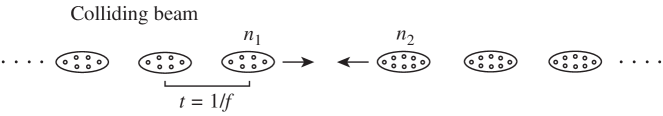
Another important parameter for a collider is the instantaneous luminosity, the number of particles passing each other per unit time through unit transverse area at the interaction point. In reality, the particle beams usually come in bunches, as roughly illustrated in Figure 1. If there are $n_{1}$ particles in each bunch in beam 1 and $n_{2}$ in each bunch in beam 2, then the collider luminosity scales as

$${\cal{L}}\propto fn_{1}n_{2}/a,$$ (8)

where $f$ is beam crossing frequency and $a$ the transverse profile of the beams. The instantaneous luminosity is usually given in units of cm^-2 s^-1.

Figure 1: Colliding beams with a bunch crossing frequency $f$.

The reaction rate, that is the number of scattering events per unit time, is directly proportional to the luminosity and is given by

$$R(s)=\sigma(s)\cal{L},$$ (9)

where $\sigma(s)$ is defined to be the total scattering cross section. Though the units of cross sections are conventionally taken as cm², these units are much too big to use for sub-atomic particle scattering, and thus more suitable units, called a barn, are introduced

$$1\ {\rm cm}^{2}=10^{24}\ {\rm barn}=10^{27}\ {\rm mb}=10^{30}\ \mu{\rm b}=10^{33}\ {\rm nb}=10^{36}\ {\rm pb}=10^{39}\ {\rm fb}=10^{42}\ {\rm ab.}$$

It may also be convenient to use these units for the luminosity accordingly like

$$1\ {\rm cm}^{-2}\ {\rm s}^{-1}=10^{-33}\ {\rm nb}^{-1}\ {\rm s}^{-1}.$$

In fact, it is often quite relevant to ask a year long accumulation of the luminosity, or an integrated luminosity over time. It is therefore useful to remember a collider’s luminosity in the units

$$10^{33}\ {\rm cm}^{-2}\ {\rm s}^{-1}=1\ {\rm nb}^{-1}\ {\rm s}^{-1}\approx 10\ {\rm fb}^{-1}/{\rm year.}$$

In practice, the instantaneous luminosity has some spread around the peak energy $\sqrt{s}$, written as $dL/d\tau$ with $\tau=\hat{s}/s$ where $\hat{s}$ is the c.m. energy squared with which the reaction actually occurs. The more general form for Eq. (9) is

$$R(s)={\cal L}\int d\tau{dL\over d\tau}\ \sigma(\hat{s}).$$ (10)

With the normalization $\int dL/d\tau\ d\tau=1$, then ${\cal L}$ is the peak instantaneous luminosity. The energy spectrum of the luminosity often can be parameterized by a Gaussian distribution with an energy spread as given by $\delta E$ ($\sim\sqrt{s}-\sqrt{\hat{s}}$) in Tables 1 and 2. For most of the purposes, the energy spread is much smaller than other energy scales of interest, so that the luminosity spectrum is well approximated by $\delta(1-\tau)$. Thus, Eq. (9) is valid after the proper convolution. The only exception would be for resonant production with a physical width narrower than the energy spread. We will discuss this case briefly in the next $e^{+}e^{-}$ collider section.

While the luminosity is a machine characteristics, the cross section is determined by the fundamental interaction properties of the particles in the initial and final states. Determining the reaction cross section and studying the scattering properties as a function of energy, momentum, and angular variables will be of ultimate importance to uncover new dynamics at higher energy thresholds.

The electrons and protons are good candidates for serving as the colliding beams. They are electrically charged so that they can be accelerated by electric field, and are stable so that they can be put in a storage ring for reuse to increase luminosity. In Table 1, we list the important machine parameters for some $e^{+}e^{-}$ colliders as well as some future machines. In Table 2, we list the important machine parameters for some colliders. Electron and proton colliders are complementary in many aspects for physics exploration, as we will discuss below.

II.2 $e^{+}e^{-}$ Colliders

The collisions between electrons and positrons have some major advantages. For instance,

• The $e^{+}e^{-}$ interaction is well understood within the standard model electroweak theory. The SM processes are predictable without large uncertainties, and the total event rates and shapes are easily manageable in the collider environments.

• The system of an electron and a positron has zero charge, zero lepton number etc., so that it is suitable to create new particles after $e^{+}e^{-}$ annihilation.

• With symmetric beams between the electrons and positrons, the laboratory frame is the same as the c.m. frame, so that the total c.m. energy is fully exploited to reach the highest possible physics threshold.

• With well-understood beam properties, the scattering kinematics is well-constrained.

• It is possible to achieve high degrees of beam polarizations, so that chiral couplings and other asymmetries can be effectively explored.

One disadvantage is the limiting factor due to the large synchrotron radiation as given in Eq. (7). The rather light mass of the electrons limits the available c.m. energy for an $e^{+}e^{-}$ collider. Also, a multi-hundred GeV $e^{+}e^{-}$ collider will have to be made a linear accelerator ILC . This in turn becomes a major challenge for achieving a high luminosity when a storage ring is not utilized. When performing realistic simulations for high energy $e^{+}e^{-},\ e^{-}e^{-}$ reactions at high luminosities, the beamstrahlung effects on the luminosity and the c.m. energy become substantial and should not be overlooked.

Another disadvantage for $e^{+}e^{-}$ collisions is that they predominantly couple to a vector (spin 1) state in $s$-channel, so that the resonant production of a spin-0 state (Higgs-like) is highly suppressed. For a higher spin state, such as spin-2, the resonant production will have to go through a higher partial wave.

Figure 2: Scattering cross sections versus c.m. energy for the SM processes in $e^{+}e^{-}$ collisioins. The Higgs boson mass has been taken as 120 GeV.

II.2.1 Production cross sections for standard model processes

For the production of two-particle $a,b$ and for unpolarized beams so that the azimuthal angle can be trivially integrated out (see Appendix A.3), the differential cross section as a function of the scattering polar angle in the c.m. frame is given by

$${d\sigma(e^{+}e^{-}\to ab)\over d\cos\theta}=\frac{\beta}{32\pi s}\overline{\sum}|{\cal M}|^{2},$$ (11)

where $\beta=\lambda^{1/2}(1,m_{a}^{2}/s,m_{b}^{2}/s)$ is the speed factor for the out-going particles, $\overline{\sum}|{\cal M}|^{2}$ is the scattering matrix element squared, summed and averaged over unobserved quantum numbers like color and spins.

It is quite common that one needs to consider a fermion pair production $e^{-}e^{+}\to f\bar{f}$. For most of the situations, the scattering matrix element can be casted into a $V\pm A$ chiral structure of the form (sometimes with the help of Fierz transformations)

$${\cal M}={e^{2}\over s}Q_{\alpha\beta}\ [\bar{v}_{e^{+}}(p_{2})\gamma^{\mu}P_{\alpha}u_{e^{-}}(p_{1})]\ [\bar{\psi}_{f}(q_{1})\gamma_{\mu}P_{\beta}\psi^{\prime}_{\bar{f}}(q_{2})],$$ (12)

where $\alpha,\beta=L,R$ are the chiral indices, $P_{L,R}=(1\mp\gamma_{5})/2$, and $Q_{\alpha\beta}$ are the chiral bilinear couplings governed by the underlying physics of the interactions with the intermediate propagating fields. With this structure, the scattering matrix element squared can be conveniently expressed as

$$\overline{\sum}|{\cal M}|^{2} = {e^{4}\over s^{2}}\left[(|Q_{LL}|^{2}+|Q_{RR}|^{2})\ u_{i}u_{j}+(|Q_{LR}|^{2}+|Q_{RL}|^{2})\ t_{i}t_{j}\right.$$ (13)

$$+ \left.2Re(Q_{LL}^{*}Q_{LR}+Q_{RR}^{*}Q_{RL})m_{f}m_{\bar{f}}s\right],$$

where $t_{i}=t-m_{i}^{2}=(p_{1}-q_{1})^{2}-m_{i}^{2}$ and $u_{i}=u-m_{i}^{2}=(p_{1}-q_{2})^{2}-m_{i}^{2}$.

Exercise: Derive Eq. (13) by explicit calculations from Eq. (12).

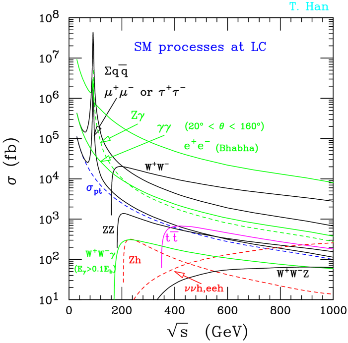
Figure 2 shows the cross sections for various SM processes in $e^{+}e^{-}$ collisions versus the c.m. energies. The simplest reaction is the QED process $e^{+}e^{-}\to\gamma^{*}\to\mu^{+}\mu^{-}$ and its cross section is given by

$${\sigma(e^{+}e^{-}\to\gamma^{*}\to\mu^{+}\mu^{-})\equiv\sigma_{pt}=\frac{4\pi\alpha^{2}}{3s}}.$$ (14)

In fact, $\sigma_{pt}\approx 100$ fb$/(\sqrt{s}/{\rm TeV})^{2}$ has become standard units to measure the size of cross sections in $e^{+}e^{-}$ collisions. However, at energies near the EW scale, the SM $Z$ boson resonant production dominates the cross section, seen as the sharp peek slightly below 100 GeV. Above the resonance, cross sections scale asymptotically as $1/s$, like the $s$-channel processes typically do. This is even true for scattering with $t,u$-channel diagrams at finite scattering angles. The only exceptions are the processes induced by collinear radiations of gauge bosons off fermions, where the total cross section receives a logarithmic enhancement over the fermion energy. For a massive gauge boson fusion process,

$$\sigma\sim{1\over M^{2}_{V}}\ln^{2}{s\over M_{V}^{2}}.$$ (15)

To have a quantitative feeling, we should know the sizes of typical cross sections at a 500 GeV ILC

$$\sigma(W^{+}W^{-})\approx 20\sigma_{pt}\approx 8\ {\rm pb};$$

$$\sigma(ZZ)\approx\sigma(t\bar{t})\approx\sigma_{pt}\approx 400\ {\rm fb};$$

$$\sigma(ZH)\approx\sigma(WW\to H)\approx\sigma_{pt}/4\approx 100\ {\rm fb};$$

$$\sigma(WWZ)\approx 0.1\ \sigma_{pt}\approx 40\ {\rm fb}.$$

Now let us treat these two important cases in more details.

II.2.2 Resonant production

The resonant production for a single particle of mass $M_{V}$, total width $\Gamma_{V}$, and spin $j$ at c.m. energy $\sqrt{s}$ is

$$\sigma(e^{+}e^{-}\to V\to X)=\frac{4\pi(2j+1)\Gamma(V\to e^{+}e^{-})\Gamma(V\to X)}{(s-M^{2}_{V})^{2}+\Gamma_{V}^{2}M_{V}^{2}}\ {s\over M_{V}^{2}},$$ (16)

where $\Gamma(V\to e^{+}e^{-})$ and $\Gamma(V\to X)$ are the partial decay widths for $V$ to decay to the initial and final sates, respectively. This is the Breit-Wigner resonance to be discussed in Eq. (100) of Appendix B. For an ideal monochromatic luminosity spectrum, or the energy spread of the machine much smaller than the physical width $\Gamma_{V}$, the above equation is valid. This is how the $Z$ resonant production cross section was calculated in Fig. 2 as a function of the c.m. energy $\sqrt{s}$, and how the $Z$ line-shape was measured by the energy-scan in the LEP I and SLC experiments.

Exercise: Verify Eq. (16) by assuming a generic vector production and decay.

It can occur that the energy spectrum of the luminosity is broader than the narrow resonant width. One could take the narrow-width approximation as given in Eq. (100) and thus the cross section is

$$\sigma(e^{+}e^{-}\to V\to X)=\frac{4\pi^{2}(2j+1)\Gamma(V\to e^{+}e^{-})BF(V\to X)}{M_{V}^{3}}\ {dL\over d\tau}|_{s=M_{V}^{2}},$$ (17)

where $dL/d\tau|_{s=M_{V}^{2}}$ presents the contribution of the luminosity at the resonant mass region . In other complicated cases when neither approximation applies between $\delta E$ and $\Gamma_{V}$, the more general convolution as in Eq. (10) may be needed. For a discussion, see e.g. the reference muon .

Exercise: Derive Eq. (17) by applying Eq. (10) with the narrow width approximation as in Eq. (100).

The resonant production is related to the $s$-channel singularity in the $S$-matrix for an on-shell particle propagation. It is the most important mechanism for discovering new particles in high energy collider experiments. We will explore in great detail the kinematical features in Sec. IV.

II.2.3 Effective photon approximation

A qualitatively different process is initiated from gauge boson radiation, typically off fermions. The simplest case is the photon radiation off an electron. For an electron of energy $E$, the probability of finding a collinear photon of energy $xE$ is given by

$$P_{\gamma/e}(x)=\frac{\alpha}{2\pi}{1+(1-x)^{2}\over x}\ln{E^{2}\over m^{2}_{e}},$$ (18)

which is known as the Weizsäcker-Williams spectrum. We see that the electron mass enters the log to regularize the collinear singularity and $1/x$ leads to the infrared behavior of the photon. These dominant features are a result of a $t$-channel singularity for the photon. This distribution can be obtained by calculating the splitting process as depicted in Fig. 3, for $e^{-}a\to e^{-}X$. The dominant contribution is induced by the collinear photon and thus can be expressed as

$$\sigma(e^{-}a\to e^{-}X)\approx\int dx\ P_{\gamma/e}(x)\ \sigma(\gamma a\to X).$$ (19)

This is also called the effective photon approximation.

This picture of the photon probability distribution in Eq. (19) essentially treats the photons as initial state to induce the reaction. It is also valid for other photon spectrum. It has been proposed recently to produce much harder photon spectrum based on the back-scattering laser techniques gamma to construct a “photon collider”. There have been dedicated workshops to study the physics opportunities for $e^{+}e^{-}$ linear colliders operating in such a photon collider mode, but we will not discuss the details further here.

Figure 3: Illustrative Feynman diagram for effective photon approximation.

A similar picture may be envisioned for the radiation of massive gauge bosons off the energetic fermions, for example the electroweak gauge bosons $V=W^{\pm},Z$. This is often called the Effective $W$-Approximation sally ; gordy . Although the collinear radiation would not be a good approximation until reaching very high energies $\sqrt{s}\gg M_{V}$, it is instructive to consider the qualitative features, which we will defer to Sec. IV.3 for detailed discussions.

II.2.4 Beam polarization

One of the merits for an $e^{+}e^{-}$ linear collider is the possible high polarization for both beams, as indicated in Table 1. Consider first the longitudinal polarization along the beam line direction. Denote the average $e^{\pm}$ beam polarization by $P^{L}_{\pm}$, with $P^{L}_{\pm}=-1$ purely left-handed and $+1$ purely right-handed. Then the polarized squared matrix element can be constructed polar based on the helicity amplitudes ${\cal M}_{\sigma_{e-}\sigma_{e+}}$

$$\overline{\sum}|{\cal M}|^{2}={1\over 4}[(1-P^{L}_{-})(1-P^{L}_{+})|{\cal M}_{--}|^{2}+(1-P^{L}_{-})(1+P^{L}_{+})|{\cal M}_{-+}|^{2}$$

$$+(1+P^{L}_{-}(1-P^{L}_{+})|{\cal M}_{+-}|^{2}+(1+P^{L}_{-})(1+P^{L}_{+})|{\cal M}_{++}|^{2}].$$ (20)

Since the electroweak interactions of the SM and beyond are chiral, it is important to notice that contributions from certain helicity amplitudes can be suppressed or enhanced by properly choosing the beam polarizations. Furthermore, it is even possible to produce transversely polarized beams with the help of a spin-rotator. If the beams present average polarizations with respect to a specific direction perpendicular to the beam line direction, $-1<P_{\pm}^{T}<1$, then there will be one additional term in Eq. (20) (in the limit $m_{e}\to 0$),

$${1\over 4}\ 2\ P^{T}_{-}P^{T}_{+}\ {\rm Re}({\cal M}_{-+}{\cal M}_{+-}^{*}).$$

The transverse polarization is particularly important when the interactions under consideration produce an asymmetry in azimuthal angle, such as the effect of CP violation.

For a comprehensive count on physics potential for the beam polarization, see a recent study in Ref. epolar .

Figure 4: An illustrative event in hadronic collisions.

II.3 Hadron Colliders

Protons are composite particles, made of “partons” of quark and gluons. The quarks and gluons are the fundamental degrees of freedom to participate in strong reactions at high energies according to QCD george . The proton is much heavier than the electron. These lead to important differences between a hadron collider and an $e^{+}e^{-}$ collider.

• Due to the heavier mass of the proton, hadron colliders can provide much higher c.m. energies in head-on collisions.

• Higher luminosity can be achieved also, by making use of the storage ring for recycle of protons and antiprotons.

• Protons participate in strong interactions and thus hadronic reactions yield large cross sections. The total cross section for a proton-proton scattering can be estimated by dimensional analysis to be about 100 mb, with weak energy-dependence.

• At higher energies, there are many possible channels open up resonant productions for different charge and spin states, induced by the initial parton combinations such as $q\bar{q}$, $qg$, and $gg$. As discussed in the last section for gauge boson radiation, there are also contributions like initial state $WW,ZZ$ and $WZ$ fusion.

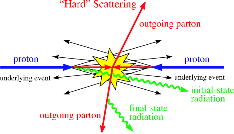
The compositeness and the strong interactions of the protons on the other hand can be disadvantageous in certain aspect, as we will see soon. An interesting event for a high-energy hadronic scattering may be illustrated by Fig. 4.

II.3.1 Hard scattering of partons

Thanks to the QCD factorization theorem, which states that the cross sections for high energy hadronic reactions with a large momentum transfer can be factorized into a parton-level “hard scattering” convoluted with the parton “distribution functions”. For scattering of two hadrons $A$ and $B$ to produce a final state $F$ of our interest, the cross section can be formally written as a sum over the sub-process cross sections from the contributing partons

$$\sigma(AB\to F\ X)=\sum_{a,b}\int dx_{1}dx_{2}\ P_{a/A}(x_{1},Q^{2})P_{b/B}(x_{2},Q^{2})\ \hat{\sigma}(ab\to F),$$ (21)

where $X$ is the inclusive scattering remnant, and $Q^{2}$ is the factorization scale (or the typical momentum transfer) in the hard scattering process, much larger than $\Lambda_{QCD}^{2}\approx(200\ {\rm MeV})^{2}$. The parton-level hard scattering cross section can be calculated perturbatively in QCD, while the parton distribution functions parameterize the non-perturbative aspect and can be only obtained by some ansatz and by ffitting the data. For more discussions, the readers are referred to George Sterman’s lectures george on QCD, or the excellent text esw on thesse topics.

Figure 5: Parton momentum distributions versus their energy fraction $x$ at two different factorization scales, from CTEQ-5.

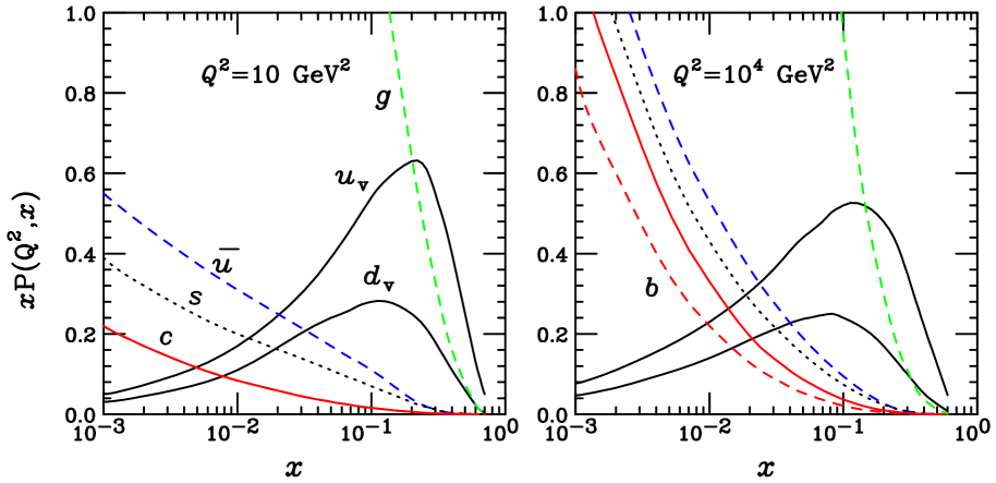
Since the QCD parton model plays a pivotal role in understanding hadron collisions and uncovering new phenomena at high energies, we plot in Fig. 5 the parton momentum distributions versus the energy fractions $x$, taking CTEQ-5 as a representative cteq5 . For comparison, we have chosen the QCD factorization scale to be $Q^{2}$=10 ${\rm GeV}^{2}$ and $10^{4}\ {\rm GeV}^{2}$ in these two panels, respectively. Several general features are important to note for future discussions. The valence quarks $u_{v},\ d_{v}$, as well as the gluons carry a large momentum fraction, typically $x\sim 0.08-0.3$. The “sea quarks” ($\bar{u}=u_{sea},\bar{d}=d_{sea},s,c,b$) have small $x$, and are significantly enhanced at higher $Q^{2}$. Both of these features lead to important collider consequences. First of all, heavy objects near the energy threshold are more likely produced via valence quarks. Second, higher energy processes (comparing to the mass scale of the parton-level subprocess) are more dominantly mediated via sea quarks and gluons.

Figure 6: Scattering cross sections versus c.m. energy for the SM processes in $pp$ collisioins. The Higgs boson mass has been taken as 120 GeV.

II.3.2 Production cross sections for standard model processes

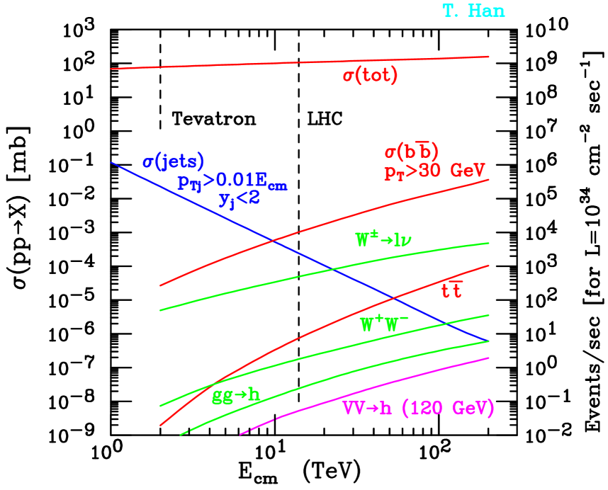
In Figure 6, we show the integrated cross sections for various typical processes in the SM versus c.m. energy of a $pp$ hadron collider in units of mb. The scale on the right-hand side gives the event rate for an instantaneous luminosity $10^{34}\ {\rm cm}^{-2}\ {\rm s}^{-1}$, a canonical value for the LHC. We have indicated the energies at the Tevatron and the LHC by the vertical dashed lines. First of all, we have plotted the $pp$ total cross section as the line on the top. It is known that the cross section increases with the c.m. energy ttwu . Unitarity argument implies that it can only increase as a power of $\ln s$. An empirical scaling relation $s^{0.09}$ gives a good fit to the measurements upto date, and has been used here.

All integrated cross sections in hadronic collisions increase with the c.m. energy due to the larger parton densities at higher energies. The jet-inclusive cross section $\sigma$(jets) is given by the blue line. The reason the cross section falls is due to our choice of an energy-dependent cut on the jet’s transverse momuntum. The $b\bar{b}$ pair production is also sensitively dependent upon the transverse momentum cutoff since the mass $m_{b}$ is vanishingly small comparing to the collider energies and thus the integrated cross section presents the familiar collinear singularity in the forward scattering region. The production at the leading order is dominantly via the gluon-initiated process $gg\to b\bar{b}$, and is of the order of 1 $\mu$b at the LHC energy (with a cutoff $p_{T}>30$ GeV). The top-quark production is again dominated by the gluon fusion, leading to about $90\%$ of the total events. The rate of the leading order prediction is about 700 pb or about 7 Hz with a canonical luminosity, and higher order QCD corrections are known to be substantial top . It is thus justifiable to call the LHC a “top-quark factory”. We also see that the leading Higgs boson production mechanism is also via the gluon fusion, yielding about 30 pb. QCD corrections again are very large, increasing the LO cross section by a significant factor ggh . Another interesting production channel is the gauge-boson fusion $VV\to h$, that is about factor of 5 smaller than the inclusive $gg\to h$ in rate, and the QCD correction is very modest vvh .

Most of the particles produced in high-energy collisions are unstable. One would need very sophisticated modern detector complex and electronic system to record the events for further analyses. We now briefly discuss the basic components for collider detectors.

III Collider Detectors: Our Electronic Eyes

Accelerators and colliders are our powerful tools to produce scattering events at high energies. Detectors are our “e-eyes” to record and identify the useful events to reveal the nature of fundamental interactions.

III.1 Particle Detector at Colliders

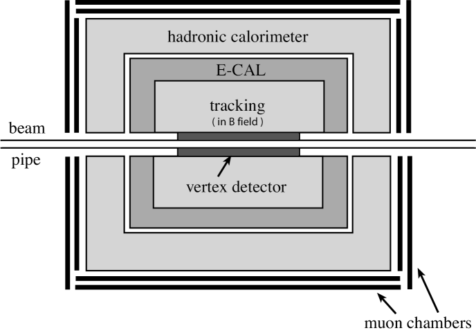
The particle detection is based on its interactions with matter of which the detectors are made. A modern particle detector is an electronic complex beyond the traditional particle detection techniques, which typically consists of a secondary displaced vertex detector/charge-tracking system, electromagnetic calorimetry, hadronic calorimetry and a muon chamber, etc.

A simplified layout is shown in Fig. 7.

Figure 7: Modern multi-purpose detector at colliders.

III.2 What Do Particles Look Like in a Detector

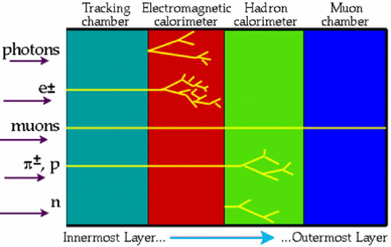
As theorists, we mostly deal with the fundamental degrees of freedom in our SM Lagrangian, namely the quarks, leptons, gauge bosons etc. in our calculations. The truth is that most of them are not the particles directly “seen” in the detectors. Heavy particles like $Z,\ W,\ t$ will promptly decay to leptons and quarks, with a lifetime $1/\Gamma\sim 1/(2\ {\rm GeV})\approx 3.3\times 10^{-25}$ s. Other quarks will fragment into color-singlet hadrons due to QCD confinement at a time scale of $t_{h}\sim 1/\Lambda_{QCD}\approx 1/(200\ {\rm MeV})\approx 3.3\times 10^{-24}$ s. The individual hadrons from fragmentation may even behave rather differently in the detector, depending on their interactions with matter and their life times. Stable paricles such as $p,\ \bar{p},\ e^{\pm},\ \gamma$ will show up in the detector as energy deposit in hadronic and electromagnetic calorimeters or charge tracks in the tracking system. In Fig. 8, we indicate what particles may leave what signatures in certain components of the detector.

Figure 8: Particle signatures left in the detector components.

In order to have better understanding for the particle observation, let us recall the decay length of an unstable particle

$$d=(\beta\ c\tau)\gamma\approx(300\ \mu m)({\tau\over 10^{-12}\ s})\ \gamma,$$ (22)

where $\tau$ is the particle’s proper lifetime and $\gamma=E/m$ is the relativistic factor. We now can comment on how particles may show up in a detector.

• Quasi-stable: fast-moving particles of a life-time $\tau>10^{-10}$ s will still interact in the detector in a similar way. Those include the weak-decay particles like the neutral hadrons $n,\Lambda,K^{0}_{L},\ ...$ and charged particles $\mu^{\pm},\ \pi^{\pm},K^{\pm},\ ...$

• Short-lived resonances: particles undergoing a decay of typical electromagnetic or strong strength, such as $\pi^{0},\ \rho^{0,\pm}$… and very massive particles like $Z,W^{\pm},t,(H...)$, will decay “instantaneously”. They can be only “seen” from their decay products and hopefully via a reconstructed resonance.

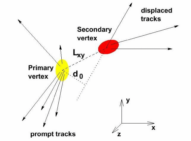
• displaced vertex: particles of a life-time $\tau\sim 10^{-12}$ s, such as $B^{0,\pm},\ D^{0,\pm},\ \tau^{\pm},$ may travel a distinguishable distance ($c\tau\sim 100\ \mu$m.) before decaying into charged tracks, and thus result in a displaced secondary vertex, as shown in Fig. 9, where the decay length between the two vertices is denoted by $L$. As an interesting and important case, $K_{S}^{0}$ with $c\tau\sim 2.7$ cm also often results in a secondary vertex via its decay to $\pi^{+}\pi^{-}$.

• Things not “seen”: those that do not participate in electromagnetic nor strong interactions, but long-lived as least like the quasi-stable particles, will escape from detection by the detector, such as the neutrinos $\nu$ and neutralinos $\tilde{\chi}^{0}$ in SUSY theories, etc.

Figure 9: An illustrative event leading to a displaced secondary vertex.

Now coming back to the elementary particles in the SM, we illustrate their behavior in Table 3. A check indicates an appearance in that component, a cross means no, a check-cross is partially yes. Other symbols are self-explained.

Leptons	Vetexing	Tracking	ECAL	HCAL	Muon Cham.
$e^{\pm}$	$\times$	$\vec{p}$	$E$	$\times$	$\times$
$\mu^{\pm}$	$\times$	$\vec{p}$	$\surd$	$\surd$	$\vec{p}$
$\tau^{\pm}$	$\surd\times$	$\surd$	$e^{\pm}$	$h^{\pm};\ 3h^{\pm}$	$\mu^{\pm}$
$\nu_{e},\nu_{\mu},\nu_{\tau}$	$\times$	$\times$	$\times$	$\times$	$\times$
Quarks
$u,d,s$	$\times$	$\surd$	$\surd$	$\surd$	$\times$
$c\to D$	$\surd$	$\surd$	$e^{\pm}$	$h$’s	$\mu^{\pm}$
$b\to B$	$\surd$	$\surd$	$e^{\pm}$	$h$’s	$\mu^{\pm}$
$t\to bW^{\pm}$	$b$	$\surd$	$e^{\pm}$	$b+2$ jets	$\mu^{\pm}$
Gauge bosons
$\gamma$	$\times$	$\times$	$E$	$\times$	$\times$
$g$	$\times$	$\surd$	$\surd$	$\surd$	$\times$
$W^{\pm}\to\ell^{\pm}\nu$	$\times$	$\vec{p}$	$e^{\pm}$	$\times$	$\mu^{\pm}$
$\quad~{}\to q\bar{q}^{\prime}$	$\times$	$\surd$	$\surd$	2 jets	$\times$
$Z^{0}\to\ell^{+}\ell^{-}$	$\times$	$\vec{p}$	$e^{\pm}$	$\times$	$\mu^{\pm}$
$\to q\bar{q}$	$(b\bar{b})$	$\surd$	$\surd$	2 jets	$\times$

Table 3: What the elementary particles in the SM look like in detectors.

III.3 More on Measurements

It is informative to discuss in a bit more detail a few main components for the particle detection. We hope to indicate how and how well the energy, momentum, and other properties of particles can be measured. When needed, we will freely take either the ATLAS or the CMS detector as an example for the purpose of illustration.

Vertexing: Normally, at least two charged tracks are needed to reconstruct a secondary decay vertex, as illustrated in Fig. 9. Note that if the decaying particle moves too fast, then the decay products will be collimated, with a typical angle $\theta\approx\gamma^{-1}=m/E$. The impact parameter $d_{0}$ as in Fig. 9 can be approximated as $d_{0}\approx L_{xy}\theta$. The impact parameter is crucial to determine the displaced vertex. For instance, the ATLAS detector ATLAS has the resolution parameterized by

$${\Delta d_{0}}=11\oplus{73\over(p_{T}/{\rm GeV})\ \sqrt{\sin\theta}}\ (\mu m),$$ (23)

where the notation $\oplus$ implies a sum in quadrature.

It is possible to resolve a secondary vertex along the longitudinal direction alone, which is particularly important if there will be only one charged track observed. In this case, the resolution is typically worse and it can be approximated ATLAS as

$${\Delta z_{0}}=87\oplus{115\over(p_{T}/{\rm GeV})\ \sqrt{\sin^{3}\theta}}\ (\mu m).$$ (24)

Tracking: Tracking chamber determines the trajectories of traversing charged particles as well as their electromagnetic energy loss $dE/dx$. The rapidity coverage is

$$|\eta_{\mu}|\approx 2.5,$$ (25)

for both ATLAS and CMS.

When combined with a magnetic field (2 T for ATLAS and 4 T for CMS), the system can be used to measure a charged particle momentum. The curvature of the trajectory is inversely proportional to the particle momentum

$$\kappa\equiv{1\over\rho}\propto{QB\over p},$$ (26)

where $Q$ is the particle’s electric charge and $B$ the external magnetic field. Therefore, knowing $B$ and assmuing a (unity) charge, the momentum $p$ can be determined.

The energy-loss measurement $dE/dx$ for heavy charged particles may be used for particle identification. For instance, the Bethe-Bloch formula for the energy loss by excitation and ionization gives a scaling quadratically with the particle charge and inversely with the speed

$${dE\over dx}\propto\left({Q\over\beta}\right)^{2},$$ (27)

independent of the charged particle mass. The mass can thus be deduced from $p$ and $\beta$. However, if we allow a most general case for a particle of arbitrary $m,Q$, then an additional measurement (such as $\beta$ from a Cerenkov counter or time-of-flight measurements) would be needed to fully determine the particle identiy.

From the relation Eq. (26), the momentum resolution based on a curvature measurement can be generically expressed as

$${\Delta p_{T}\over p_{T}}={ap_{T}}\oplus{b},$$ (28)

For instance, the ATLAS ATLAS (CMS CMS ) detector has the resolution parameterized by $a=36\%\ {\rm TeV}^{-1}\ \ (15\%\ {\rm TeV}^{-1}),\ b=1.3\%/\sqrt{\sin\theta}\ \ (0.5\%)$. In particular, the momentum resolution for very high energy muons about $p_{T}\approx 1$ TeV in the central region can reach $10\%\ (6\%)$ for ATLAS (CMS). Good curvature resolution for highly energetic particle’s tracks is important for the charge determination.

ECAL: High-energy electrons and photons often lead to dramatic cascade electromagnetic showers due to bremsstrahlung and pair production. The number of particles created increase exponentially with the depth of the medium. Since the incident energy to be measured by the electromagnetic calorimetry (ECAL) is proportional to the maximum number of particles created, the energy resolution is characterized by $1/\sqrt{N}$, often parameterized by

$${\Delta E\over E}={a\over\sqrt{E/{\rm GeV}}}\oplus{b},$$ (29)

where $a$ is determined by the Gaussian error and $b$ the response for cracks. For ATLAS (CMS), $a=10\%\ \ (5\%),\ \ b=0.4\%\ \ (0.55\%)$.

The coverage in the rapidity range can reach

$$|\eta_{e,\gamma}|\approx 3$$ (30)

or slightly over for both ATLAS and CMS.

HCAL: Similar to the ECAL, showers of subsequent hadrons can be developed from the high-energy incident hadrons. An HCAL is to measure the hadronic energy, and the Gaussian error again is parameterized as

$${\Delta E\over E}={a\over\sqrt{E}}\oplus{b}.$$ (31)

For ATLAS (CMS), $a=80\%\ \ (100\%),\ \ b=15\%\ \ (5\%)$.

The rapidity coverage by the forward hadronic calorimeter can reach

$$|\eta_{h}|\approx 5$$ (32)

for both ATLAS and CMS.

III.4 Triggering

So far, we have ignored one very important issue: data acquisition and triggering. Consider $pp$ collisions at the LHC energies, the hadronic total cross section is of the order about 100 mb, and the event rate at the designed luminosity ($10^{34}$ cm^-2 s^-1) will be about 1 GHz (compare with the clock speed of your fast computer processor). A typical even will take about one Mega bytes of space. It is therefore impossible for the detector electronic system to record the complex events of such a high frequency. Furthermore, the physical processes of our interest occur at a rate of $10^{-6}$ lower or more. Thus, one will have to be very selective in recording events of our interest. In contrast, there will be no such problems at $e^{+}e^{-}$ colliders due to the much lower reaction rate.

Trigger is the decision-making process using a desired temporal and spatial correlation in the detector signals. It is provided by examining the properties of the physical process as appeared in the detector. Modern detectors for hadron colliders such as CDF, D0 at the Tevatron and ATLAS, CMS at the LHC typically adopt three levels of triggering. At the LHC experiments, Level-1 triggering brings the event rate down to the order of $10^{5}$ Hz; Level-2 to about $10^{3}$ Hz; and Level-3 finally to about 100 Hz to tape.

There are many means to design a trigger, such as particle identification, multiplicity, kinematics, and event topology etc. Modern detectors at colliders usually can trigger on muons by a muon chamber, electrons/photons as electromagnetic objects, $\tau$/hadrons and jets as hadronic objects, global energy sum and missing transverse energy, and some combinations of the above.

	ATLAS
Objects	$\eta$	$p_{T}$ (GeV)
$\mu$ inclusive	2.4	6 (20)
$e$/photon inclusive	2.5	17 (26)
Two $e$’s or two photons	2.5	12 (15)
1-jet inclusive	3.2	180 (290)
3 jets	3.2	75 (130)
4 jets	3.2	55 (90)
$\tau$/hadrons	2.5	43 (65)
$\hbox to0.0pt{\hbox to7.95831pt{\hfil/\hfil}\hss}E_{T}$	4.9	100
Jets$+\hbox to0.0pt{\hbox to7.95831pt{\hfil/\hfil}\hss}E_{T}$	3.2, 4.9	50,50 (100,100)

Table 4: Level-1 trigger thresholds in $\eta$-$p_{T}$ coverage for the ATLAS ATLAS detector. Entries are for a luminosity of $10^{33}$ cm^-2 s^-1 ($10^{34}$ cm^-2 s^-1 in parentheses).

Relevant to collider phenomenology is to know what particles may be detected in what kinematical region usually in $p_{T}$-$\eta$ coverage, as the detector’s acceptance for triggering purposes. Table 4 summarizes Level-1 trigger thresholds for ATLAS for the commonly observed objects and some useful combinations.

Inversely, if we find some trigger designs inadequate for certain physics needs, such as a well-motivated new physics signal with exotic characteristics or unusual kinematics, it is the responsibility of our phenomenologists to communicate with our experimental colleagues to propose new trigger designs.

IV Uncover New Dynamics at Colliders

Instead of summarizing which new physics scenario can be covered by which collider to what extent, I would like to discussion a few examples for observing signals to illustrate the basic techniques and the use of kinematics. The guiding principles are simple: maximally and optimally make use of the experimentally accessible observables to uncover new particles and to probe their interactions. In designing the observables, one will need to concern their theoretical properties, like under Lorentz transformation, charge and $C,P,T$ discrete symmetries etc., as well as their experimental feasibility, like particle identification, detector acceptance and resolutions etc. I hope that this serves the purpose to stimulate reader’s creativity to cleverly exploit kinematics to reveal new dynamics in collider experiments.

IV.1 Kinematics at Hadron Colliders

In performing parton model calculations for hadronic collisions like in Eq. (21), the partonic c.m. frame is not the same as the hadronic c.m. frame, e. g. the lab frame for the collider. Consider a collision between two hadrons of $A$ and $B$ of four-momenta $P_{A}=(E_{A},0,0,p_{A})$ and $P_{B}=(E_{A},0,0,-p_{A})$ in the lab frame. The two partons participating the subprocess have momenta $p_{1}=x_{1}P_{A}$ and $p_{2}=x_{2}P_{B}$. The parton system thus moves in the lab frame with a four-momentum

$$P_{cm}=[(x_{1}+x_{2})E_{A},\ 0,\ 0,\ (x_{1}-x_{2})p_{A}]\quad(E_{A}\approx p_{A}),$$ (33)

or with a speed $\beta_{cm}=(x_{1}-x_{2})/(x_{1}+x_{2})$, or with a rapidity

$$y_{cm}={1\over 2}\ln{x_{1}\over x_{2}}.$$ (34)

Denote the total hadronic c.m. energy by $S=4E_{A}^{2}$ and the partonic c.m. energy by $s$, we have

$$s\equiv\tau S,\quad\tau=x_{1}x_{2}={s\over S}.$$ (35)

The parton energy fractions are thus given by

$$x_{1,2}=\sqrt{\tau}\ e^{\pm y_{cm}}.$$ (36)

One always encounters the integration over the energy fractions as in Eq. (21). With this variable change, one has

$$\int_{\tau_{0}}^{1}dx_{1}\int_{\tau_{0}/x_{1}}^{1}dx_{2}=\int_{\tau_{0}}^{1}d\tau\int_{{1\over 2}\ln\tau}^{-{1\over 2}\ln\tau}dy_{cm}.$$ (37)

The variable $\tau$ characterizes the (invariant) mass of the reaction, with $\tau_{0}=m^{2}_{res}/S$ and $m_{res}$ is the threshold for the parton level final state (sum over the masses in the final state); while $y_{cm}$ specifies the longitudinal boost of the partonic c.m. frame with respect to the lab frame. It turns out that the $\tau-y_{cm}$ variables are better for numerical evaluations, in particular with a resonance as we will see in a later section.

Consider a final state particle of momentum $p^{\mu}=(E,\vec{p})$ in the lab frame. Since the c.m. frame of the two colliding partons is a priori undetermined with respect to the lab frame, the scattering polar angle $\theta$ in these two frames is not a good observable to describe theory and the experiment. It would be thus more desirable to seek for kinematical variables that are invariant under unknown longitudinal boosts.

Transverse momentum and the azimuthal angle:  Since the ambiguous motion between the parton c.m. frame and the hadron lab frame is along the longitudinal beam direction ($\vec{z}$), variables involving only the transverse components are invaraint under longitudinal boosts. It is thus convenient, in contrast to Eqs. (86) and (89) of Appendix A in the spherical coordinate, to write the phase space element in the cylindrical coordinate as

$${d^{3}\vec{p}\over E}=dp_{x}dp_{y}{dp_{z}\over E}=p_{T}dp_{T}d\phi\ {dp_{z}\over E},$$ (38)

where $\phi$ is the azimuthal angle about the $\vec{z}$ axis, and

$$p_{T}=\sqrt{p_{x}^{2}+p_{y}^{2}}=p\sin\theta$$ (39)

is the transverse momentum. It is obvious that both $p_{T}$ and $\phi$ are boost-invariant, so is $dp_{z}/E$.

Exercise: Prove that $dp_{z}/E$ is longitudinally boost-invariant.

Rapidity and pseudo-rapidity:  The rapidity of a particle of momentum $p^{\mu}$ is defined to be

$$y={1\over 2}\ln{E+p_{z}\over E-p_{z}}.$$ (40)

Exercise: With the introduction of rapidity $y$, show that a particle four-momentum can be rewritten as

$$p^{\mu}=(E_{T}\cosh y,p_{T}\sin\phi,p_{T}\cos\phi,E_{T}\sinh y),\quad E_{T}=\sqrt{p_{T}^{2}+m^{2}}.$$ (41)

The phase space element then can be expressed as

$${d^{3}\vec{p}\over E}=p_{T}dp_{T}d\phi\ dy=E_{T}dE_{T}d\phi\ dy.$$ (42)

Consider the rapidity in a boosted frame (say the parton c.m. frame), and perform the Lorentz transformation as in Eq. (84) of Appendix A,

$$y^{\prime}={1\over 2}\ln{E^{\prime}+p^{\prime}_{z}\over E^{\prime}-p^{\prime}_{z}}={1\over 2}\ln{(1-\beta_{0})(E+p_{z})\over(1+\beta_{0})(E-p_{z})}=y-y_{0}.$$ (43)

In the massless limit, $E\approx|{\vec{p}}|$, so that

$$y\to{1\over 2}\ln{1+\cos\theta\over 1-\cos\theta}=\ln{\cot{\theta\over 2}}\equiv\eta,$$ (44)

where $\eta$ is the pseudo-rapidity, which has one-to-one correspondence with the scattering polar angle $\pi\geq\theta\geq 0$ for $-\infty<\eta<\infty$.

Since $y$ as well as $\eta$ is additive under longitudinal boosts as seen in Eq. (43), the rapidity difference $\Delta y=y_{2}-y_{1}=y^{\prime}_{2}-y^{\prime}_{1}$ is invariant in the two frames. Thus the shape of rapidity distributions $d\sigma/dy$ in the two frames would remain the same if the boost is by a constant velocity. In realistic hadronic collisions, the boost of course varies on an event-by-event basis according to Eq. (34) and the distribution is generally smeared.

Figure 10: A CDF di-jet event on a lego plot in the $\eta-\phi$ plane. The height presents the transverse energy scale, and the two colors (blue and pink) indicate the energy deposit in the two calorimeters (ECAL and HCAL).

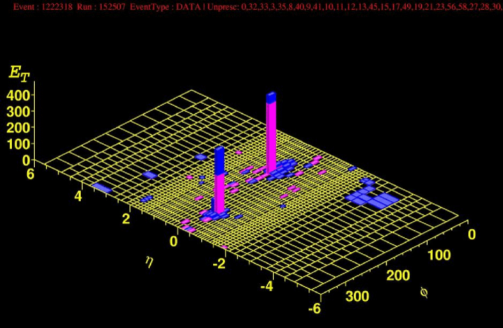
The lego plot: It should be clear by now that it is desirable to use the kinematical variables $(p_{T},\eta,\phi)$ to describe events in hadronic collisions. In collider experiments, most often, electromagnet and hadronic calorimeters provide the energy measurements for (essentially) massless particles, such as $e^{\pm},\ \gamma,$ and light quark or gluon jets. Thus

$$E_{T}=p_{T}=E\cos\theta=E\cosh^{-1}\eta.$$ (45)

A commonly adopted presentation for an electromagnetic or hadronic event is on an $\eta-\phi$ plane with the height to indicate the transverse energy deposit $E_{T}$, called the Lego plot. We show one typical di-jet event from CDF by a lego plot in Fig. 10. Of particular importance for a lego plot is that the separation between to objects on the plot is invariant under longitudinal boosts. This is seen from the definition of separation

$$\Delta R=\sqrt{\Delta\eta^{2}+\Delta\phi^{2}}.$$ (46)

As a quantitative illustration, for two objects back-to-back in the central region, typically $\Delta\eta<\Delta\phi$ and $\Delta R\approx\Delta\phi\sim\pi$.

Another important consequence for the introduction of separation is that it provides a practical definition of a hadronic jet, and $\Delta R$ specifies the cone size of a jet formed by multiple hadrons within $\Delta R$.

IV.2 $s$-channel Singularity: Resonance Signals

IV.2.1 The invariant mass variable

Searching for a resonant signal in the $s$-channel has been the most effective way of discovering new particles. Consider an unstable particle $V$ produced by $a+b$ and decaying to $1+2+...+n$. For a weakly coupled particle $\Gamma_{V}\ll M_{V}$, according to the Breit-Wigner resonance Eq. (100), the amplitude develops a kinematical peak near the pole mass value at

$$(p_{a}+p_{b})^{2}=(\ \sum_{i}^{n}p_{i}\ )^{2}\approx M_{V}^{2}.$$ (47)

This is called the invariant mass, and is the most effective observable for discovering a resonance if either the initial momenta or the final momenta can be fully reconstructed.

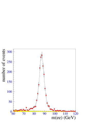
As a simple example of a two-body decay, consider $Z\to e^{+}e^{-}$,

$$m_{ee}^{2}=(p_{e^{+}}+p_{e^{-}})^{2}\approx 2p_{e^{+}}\cdot p_{e^{-}}\approx 2E_{e^{+}}E_{e^{-}}(1-\cos\theta_{e^{+}e^{-}})\approx M_{Z}^{2},$$ (48)

which is invariant in any Lorentz frame, and leads to $E_{e}\approx M_{Z}/2$ in the $Z$-rest frame. Figure 11 shows the peak in the $e^{+}e^{-}$ invariant mass spectrum at $M_{Z}$, indicating the resonant $Z$ production observed by the D0 collaboration d0 at the Tevatron collider.

Now let us examine the transverse momentum variable of a daughter particle $p_{eT}=p_{e}\sin\theta^{*}$, where $\theta^{*}$ is the polar angle in the partonic c.m. frame. For a two-body final state kinematics, we thus have

$${d\hat{\sigma}\over dp_{eT}}={4p_{eT}\over s\sqrt{1-4p_{eT}^{2}/s}}\ {d\hat{\sigma}\over d\cos\theta^{*}}.$$ (49)

The integrand is singular at $p_{eT}^{2}=s/4$, but it is integrable. Exercise: Verify this equation for Drell-Yan production of $e^{+}e^{-}$. Combining with the Breit-Wigner resonance, we obtain

$${d\hat{\sigma}\over dm_{ee}^{2}\ dp_{eT}^{2}}\propto\frac{\Gamma_{Z}M_{Z}}{(m^{2}_{ee}-M^{2}_{Z})^{2}+\Gamma_{Z}^{2}M_{Z}^{2}}\ {1\over m_{ee}^{2}\sqrt{1-4p_{eT}^{2}/m_{ee}^{2}}}\ {d\hat{\sigma}\over d\cos\theta^{*}}.$$ (50)

We see that the mass peak of the resonance leads to an enhanced distribution near $p_{eT}=M_{Z}/2$. This is called the Jacobian peak. This feature is present for any two-body kinematics with a fixed subprocess c.m. energy.

Figure 11: The resonant signal for a $Z$ boson via $Z\to e^{+}e^{-}$ at the D0 detector.

Exercise: While the invariant mass distribution $d\sigma/dm_{e^{+}e^{-}}$ is unaffected by the motion of the produced $Z$ boson, show that the $d\sigma/dp_{eT}$ distribution for a moving $Z$ with a momentum $\vec{p}_{Z}$ is changed with respect to a $Z$ at rest at the leading order of $\vec{\beta}_{Z}=\vec{p}_{Z}/E_{Z}$.

It is straightforward to generalize the invariant mass variable to multi-body system. Consider a slightly more complicated signal of a Higgs decay

$$H\to Z_{1}Z_{2}\to e^{+}e^{-}\ \mu^{+}\mu^{-}.$$ (51)

Obviously, besides the two $Z$ resonant decays, the four charged leptons should reconstruct the mass of the parent Higgs boson

$$m_{H}^{2} = (\ \sum_{i}^{4}p_{i}\ )^{2}=2(M_{Z}^{2}+p_{Z_{1}}\cdot p_{Z_{2}})$$ (52)

$$= (E_{e^{+}}+E_{e^{-}}+E_{\mu^{+}}+E_{\mu^{-}})^{2}-(\vec{p}_{e^{+}}+\vec{p}_{e^{-}}+\vec{p}_{\mu^{+}}+\vec{p}_{\mu^{-}})^{2}.$$ (53)

IV.2.2 The transverse mass variable

As another example of a two-body decay, consider $W\to e\nu$. The invariant mass of the leptonic system is

$$m_{e\nu}^{2}=(E_{e}+E_{\nu})^{2}-(\vec{p}_{eT}+\vec{p}_{\nu T})^{2}-(p_{ez}+p_{\nu z})^{2}.$$ (54)

The neutrino cannot be directly observed by the detector and only its transverse momentum can be inferred by the imbalancing of the observed momenta,

$$\vec{\hbox to0.0pt{\hbox to5.03125pt{\hfil/\hfil}\hss}p_{T}}=-\sum\vec{p_{T}}(observed),$$ (55)

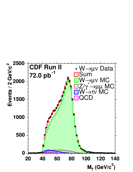
called missing transverse momentum, identified as $\hbox to0.0pt{\hbox to5.03125pt{\hfil/\hfil}\hss}p_{T}=p_{\nu T}$. Missing transverse energy is similarly defined, and $\hbox to0.0pt{\hbox to7.95831pt{\hfil/\hfil}\hss}E_{T}=E_{\nu}$. The invariant mass variable thus cannot be generally reconstructed. We would get the correct value of $m_{e\nu}$ if we could evaluate it in a frame in which the missing neutrino has no longitudinal motion $p_{\nu z}=0$; but this is impractical. Instead, one may consider to ignore the (unkown) longitudinal motion of the leptonic system (or the $W$ boson) all together, and define a transverse mass of the system MT

$$m_{e\nu T}^{2} = (E_{eT}+E_{\nu T})^{2}-(\vec{p}_{eT}+\vec{p}_{\nu T})^{2}$$

$$\approx 2\vec{p}_{eT}\cdot\vec{p}_{\nu T}\approx 2E_{eT}\hbox to0.0pt{\hbox to7.95831pt{\hfil/\hfil}\hss}E_{T}\ (1-\cos\phi_{e\nu}),$$

where $\phi_{e\nu}$ is the opening angle between the electron and the neutrino in the transverse plane. When a $W$ boson is produced with no transverse motion, $E_{eT}=\hbox to0.0pt{\hbox to7.95831pt{\hfil/\hfil}\hss}E_{T}=m_{e\nu T}/2.$ It is easy to see that the transverse mass variable is invariant under longitudinal boosts, and it reaches the maximum $m_{e\nu T}=m_{e\nu}$, for $p_{ez}=p_{\nu z}$, so that there is no longitudinal motion for the electron and the neutrino when boosting to the $W$-rest frame. In general,

$$0\leq m_{e\nu T}\leq m_{e\nu}.$$ (57)

The Breit-Wigner resonance at $m_{e\nu}=M_{W}$ naturally leads to a kinematical peak near $m_{e\nu T}\approx M_{W}$ again due to the Jacobian factor

$${d\hat{\sigma}\over dm_{e\nu}^{2}\ dm^{2}_{e\nu,T}}\propto\frac{\Gamma_{W}M_{W}}{(m^{2}_{e\nu}-M^{2}_{W})^{2}+\Gamma_{W}^{2}M_{W}^{2}}\ {1\over m_{e\nu}\sqrt{m_{e\nu}^{2}-m_{e\nu,T}^{2}}}.$$ (58)

In the narrow width approximation, $m_{e\nu T}$ is cut off sharply at $M_{W}$. In practice, the distribution extends beyond $M_{W}$ because of the finite width $\Gamma_{W}$. This is shown in Fig. 12 as observed by the CDF collaboration cdf in the channel $W\to\mu\nu$.

Figure 12: The transverse mass peak for a $W\to\mu\nu$ signal observed at CDF.

Exercise: While the invariant mass distribution $d\sigma/dm_{e\nu}$ is unaffected by the motion of the produced $W$ boson, show that the $d\sigma/dm_{e\nu T}$ distribution for a moving $W$ with a momentum $\vec{p}_{W}$ is changed with respect to a $W$ at rest at the next-to-leading order of $\vec{\beta}_{W}=\vec{p}_{W}/E_{W}$. Compare this conclusion with that obtained for $d\sigma/dp_{eT}$.

IV.2.3 The cluster transverse mass variable

A transverse mass variable with more than two-body final state is less trivial to generalize than the invariant mass variable as given in Eq. (53). This is mainly due to the fact that for a system with more than one missing neutrino, even their transverse momenta $p_{\nu_{i}T}$ cannot be individually reconstructed in general, rather, only one value $\hbox to0.0pt{\hbox to5.03125pt{\hfil/\hfil}\hss}p_{T}$ is experimentally determined, which is identified as the vector sum of all missing neutrino momenta. Thus the choice of the transverse mass variable depends on our knowledge about the rest of the kinematics, on how to cluster the other momenta, in particular realizing the intermediate resonant particles.

$H\to W_{1}W_{2}\to q_{1}\bar{q}_{2}\ e\nu$:

As the first example of the transverse mass variable with multi-body final state, let us consider a possible Higgs decay mode to $WW$ with one $W$ subsequently decaying to $q_{1}\bar{q}_{2}$ and the other to $e\nu$. Since there is only one missing neutrino, one may construct the transverse mass variable in a straightforward manner according to the kinematics for the two on-shell $W$ bosons

$$M_{T,WW}^{2} = (E_{T,W_{1}}+E_{T,W_{2}})^{2}-(\vec{p}_{T,W_{1}}+\vec{p}_{T,W_{2}})^{2}$$

$$= \left(\sqrt{p_{T,jj}^{2}+M_{W}^{2}}+\sqrt{p_{T,e\nu}^{2}+M_{W}^{2}}\right)^{2}-(\vec{p}_{T,jje}+\vec{\hbox to0.0pt{\hbox to5.03125pt{\hfil/\hfil}\hss}p_{T}})^{2}.$$

Note that if the decaying Higgs boson has no transverse motion (like being produced via $gg$ fusion), then the last term vanishes $\vec{\hbox to0.0pt{\hbox to5.03125pt{\hfil/\hfil}\hss}p_{T}}=-\vec{p}_{T,jje}.$

However, this simple construction would not be suitable for a light Higgs boson when one of the $W$ bosons (or both) is far-off shell. The above expression can thus be revised as

$$M_{T,WW}^{\prime 2}=\left(\sqrt{p_{T,jj}^{2}+m_{jj}^{2}}+\sqrt{p_{T,e\nu}^{2}+m_{e\nu T}^{2}}\right)^{2}-(\vec{p}_{T,jje}+\vec{\hbox to0.0pt{\hbox to5.03125pt{\hfil/\hfil}\hss}p_{T}})^{2}.$$

Alternatively, one can consider to combine the observed two jets and a lepton together into a cluster, and treat the missing neutrino separately. One has

$$M_{T,WW}^{\prime\prime 2}=\left(\sqrt{p_{T,jje}^{2}+M_{jje}^{2}}+\hbox to0.0pt{\hbox to5.03125pt{\hfil/\hfil}\hss}p_{T}\right)^{2}-(\vec{p}_{T,jje}+\vec{\hbox to0.0pt{\hbox to5.03125pt{\hfil/\hfil}\hss}p_{T}})^{2}.$$

Which one of those $M_{T}$ variables is the most suitable choice for the signal depends on which leads to the best Higgs mass reconstruction and a better signal-to-background ratio after simulations.

$H\to Z_{1}Z_{2}\to e^{+}e^{-}\ \nu\bar{\nu}$:

In searching for this signal, we define the cluster transverse mass based on our knowledge about the $Z$ resonances MTH ,

$$M_{T,ZZ}^{2} = (E_{T,Z_{1}}+E_{T,Z_{2}})^{2}-(\vec{p}_{T,Z_{1}}+\vec{p}_{T,Z_{2}})^{2}$$

$$= \left(\sqrt{p_{T,e^{+}e^{-}}^{2}+M_{Z}^{2}}+\sqrt{{\hbox to0.0pt{\hbox to5.03125pt{\hfil/\hfil}\hss}p_{T}}^{2}+M_{Z}^{2}}\right)^{2}-(\vec{p}_{T,e^{+}e^{-}}+\vec{\hbox to0.0pt{\hbox to5.03125pt{\hfil/\hfil}\hss}p_{T}})^{2}.$$

If the parent particle ($H$) is produced with no transverse motion, then $M_{T,ZZ}\approx 2\sqrt{p_{T,e^{+}e^{-}}^{2}+M_{Z}^{2}}.$

Exercise: Consider how to revise the above $M_{T,ZZ}$ construction if $m_{H}<2M_{Z}$ in order to better reflect the Higgs resonance.

$H\to W_{1}W_{2}\to\ell_{1}\nu_{1}\ \ell_{2}\nu_{2}$:

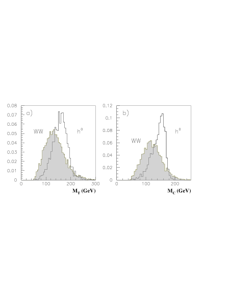
As the last example, we consider a complicated case in which the two neutrinos come from two different decays. The two missing neutrinos do not present a clear structure, and thus one simple choice may be to cluster the two charged leptons together CMT

$$M_{C,WW}^{2}=\left(\sqrt{p_{T,\ell\ell}^{2}+M_{\ell\ell}^{2}}+\hbox to0.0pt{\hbox to5.03125pt{\hfil/\hfil}\hss}p_{T}\right)^{2}-(\vec{p}_{T,\ell\ell}+\vec{\hbox to0.0pt{\hbox to5.03125pt{\hfil/\hfil}\hss}p_{T}})^{2}.$$ (59)

It was argued that since $\vec{\hbox to0.0pt{\hbox to5.03125pt{\hfil/\hfil}\hss}p_{T}}\approx-\vec{p}_{T,\ell\ell}$, thus one should have, on average, $E_{T,\nu\nu}\approx E_{T,\ell\ell}$. This leads to a different construction Herbi

$$M_{T,WW}\approx 2\sqrt{p_{T,\ell\ell}^{2}+M_{\ell\ell}^{2}}.$$ (60)

These two choices are shown in Fig. 13, for $m_{H}=170$ GeV at the Tevatron, along with the SM $WW$ background HanZhang .

Figure 13: Normalized distributions ${1\over\sigma}{d\sigma\over dM}$ for $m_{H}=170$ GeV (histogram) and the leading $WW$ background (shaded) at the Tevatron for (a) $M_{T}$ in Eq. (60) and (b) $M_{C}$ in Eq. (59).

IV.3 $t$-channel Enhancement: Vector Boson Fusion

A qualitatively different process is initiated from gauge boson radiation, typically off energetic fermions, as introduced in Sec. II.2.3. Consider a fermion $f$ of energy $E$, the probability of finding a (nearly) collinear gauge boson $V$ of energy $xE$ and transverse momentum $p_{T}$ (with respect to $\vec{p}_{f}$) is approximated by sally ; gordy

$$P^{T}_{V/f}(x,p_{T}^{2}) = \frac{g_{V}^{2}+g_{A}^{2}}{8\pi^{2}}\ {1+(1-x)^{2}\over x}\ {p_{T}^{2}\over(p_{T}^{2}+(1-x)M_{V}^{2})^{2}},$$ (61)

$$P^{L}_{V/f}(x,p_{T}^{2}) = \frac{g_{V}^{2}+g_{A}^{2}}{4\pi^{2}}\ {1-x\over x}\ {(1-x)M_{V}^{2}\over(p_{T}^{2}+(1-x)M_{V}^{2})^{2}},$$ (62)

which $T\ (L)$ denotes the transverse (longitudinal) polarization of the massive gauge boson. In the massless limit of the gauge boson, Eq. (61) reporduces the Weizsäcker-Williams spectrum as in Eq. (18), after integration of $p_{T}^{2}$ resulting in the logarithmic enhancement over the fermion beam energy. In fact, the kernel of this distribution is the same as the quark splitting function $q\to qg^{*}$ esw ; george .

The scattering cross section can thus be formally expressed as

$$\sigma(fa\to f^{\prime}X)\approx\int dx\ dp_{T}^{2}\ P_{V/f}(x,p_{T}^{2})\ \sigma(Va\to X).$$ (63)

This is also called the Effective $W$ Approximation. Although this may not be a good approximation until the parton energy reaches $E\gg M_{V}$, it is quite important to explore the general features of the $t$-channel behavior.

First of all, due to the non-zero mass of the gauge boson, there is no more collinear singularity. The typical value of the transverse momentum (gauge boson or jet) is $p_{T}\sim\sqrt{1-x}\ M_{V}\mathrel{\raise 1.29167pt\hbox{$<$\kern-7.5pt\lower 4.30554pt\hbox{$\sim$}}}M_{W}$. Since $x$ prefers to be low reflecting the infrared behavior, the jet energy $(1-x)E$ tends to be high. These observations provide the arguments for “forward jet-tagging” for massive gauge boson radiation processes: a highly energetic companion jet with $p_{T}\mathrel{\raise 1.29167pt\hbox{$<$\kern-7.5pt\lower 4.30554pt\hbox{$\sim$}}}M_{W}/2$ and a scatteirng polar angle of a few degrees jettag . Furthermore, it is very interesting to note the qualitative difference between $P^{T}$ and $P^{L}$ for the $p_{T}$ dependence (or equivalently the angular dependence) of the outgoing fermion. For $p_{T}\ll M_{W}$, $P^{T}$ is further suppressed with respect to $P^{L}$; while for $p_{T}>M_{W}$, $P^{T}$ is enhanced instead in the central scattering region. This was the original design for a forward jet-tagging and a “central jet-vetoing” tagveto to enhance the longitudinal gauge boson fusion with respect to the transverse gauge boson fusion in the search for strong $WW$ scattering signals baggeretal . It has been further realized that the $t$-channel electroweak gauge boson mediations undergo color singlet exchanges, and thus do not involve significant QCD radiation. Consequently, there will be little hadronic activities connecting the two parton currents. This further justifies the central jet-vetoing, and is developed into a “mini-jet vetoing” to further separate the gauge boson fusion processes from the large SM backgrounds in particular those with QCD radiation in the central region dieter .

IV.4 Forward-Backward Asymmetry

The precision test of universal chiral couplings of the gauge bosons $Z^{0},\ W^{\pm}$ to SM fermions is among the most crucial experimental confirmation for the validity of the SM. Similar probe would be needed to comprehend any new vector bosons once they are discovered in future collider experiments. The forward-backward asymmetry, actually the Parity-violation along the beam direction, is very sensitive to the chiral structure of the vector boson to fermion couplings.

Consider a parton-level process for a vector boson production and decay

$$i\bar{i}\to V\to f\bar{f},$$ (64)

where the initial state $i\bar{i}=e^{-}e^{+},\ q\bar{q}$. Let us now parameterize the coupling vertex of a vector boson $V_{\mu}$ to an arbitrary fermion pair $f$ by

$$i\sum_{\tau}^{L,R}g_{\tau}^{f}\ \gamma^{\mu}\ P_{\tau}.$$ (65)

Then the parton-level forward-backward asymmetry is defined as

$$A^{i,f}_{FB}\equiv\frac{N_{F}-N_{B}}{N_{F}+N_{B}}=\frac{3}{4}\mathcal{A}_{i}\mathcal{A}_{f},$$ (66)

where $N_{F}$ ($N_{B}$) is the number of events with the final-state fermion momentum $\vec{p}_{f}$ in the forward (backward) direction defined in the parton c.m. frame relative to the initial-state fermion $\vec{p}_{i}$. The asymmetry $\mathcal{A}_{f}$ is given in terms of the chiral couplings as

$$\mathcal{A}_{f}=\frac{(g_{L}^{f})^{2}-(g_{R}^{f})^{2}}{(g_{L}^{f})^{2}+(g_{R}^{f})^{2}}.$$ (67)

The formulation so far is perfectly feasible in $e^{+}e^{-}$ collisions. However, it becomes more involved when applied to hadron colliders $AB\to VX\to f\bar{f}X.$ The first problem is the mismatch between the parton c.m. frame (where the scattering angle is defined to calculate the asymmetry) and the lab frame (where the final-state fermion momentum is actually measured). This can be resolved if we are able to fully determine the final state momenta $p_{f},\ p_{\bar{f}}$. We thus construct the vector boson momentum

$$p_{V}=p_{f}+p_{\bar{f}},$$ (68)

and then boost $\vec{p}_{f}$ back to the $V$-rest frame, presumably the parton c.m. frame. The second problem is the ambiguity of the $\vec{p}_{i}$ direction: both a quark and an anti-quark as initial beams can come from either hadrons $A$ or $B$, making the determination of $\vec{p}_{i}$ impossible in general. Fortunately, one can resolve this ambiguity to a good approximation. This has something to do with our understanding for quark parton distributions in hadrons. We first recognize that for a heavy vector boson production, the parton energy fraction is relatively large $x\sim M_{V}/\sqrt{s}$, and thus the contributions from valance quarks dominate, recall Fig. 5. Consider the case at the Tevatron for $p\bar{p}$ collisions, we can thus safely choose the beam direction of the protons (with more quarks) as $\vec{p}_{i}$. As for the LHC with $pp$ collisions, this discrimination of $p$ versus $\bar{p}$ is lost. However, we note that for $u\bar{u},\ d\bar{d}$ annihilations, valance quarks ($u,\ d$) carry much larger an $x$ fraction than the anti-quark in a proton. We thus take the quark momentum direction $\vec{p}_{i}$ along with the boosted direction as reconstructed in Eq. (68), recall the boost relation Eq. (34). With those clarifications, we can now define the hadronic level asymmetry at the LHC Rosner

$$A_{FB}^{\rm LHC}=\frac{\int dx_{1}\sum_{q=u,d}A_{FB}^{q,f}\left(P_{q}(x_{1})P_{\bar{q}}(x_{2})-P_{\bar{q}}(x_{1})P_{q}(x_{2})\right){\rm sign}(x_{1}-x_{2})}{\int dx_{1}\sum_{q=u,d,s,c}\left(P_{q}(x_{1})P_{\bar{q}}(x_{2})+P_{\bar{q}}(x_{1})P_{q}(x_{2})\right)},$$ (69)

where $P_{q}(x_{1})$ is the parton distribution function for quark $q$ in the proton with momentum fraction $x_{1}$, evaluated at $Q^{2}=M_{V}^{2}$. The momentum fraction $x_{2}$ is related to $x_{1}$ by the condition $x_{1}x_{2}=M_{V}^{2}/s$ in the narrow-width approximation. Only $u$ and $d$ quarks contribute to the numerator since we explicitly take the quark and antiquark PDFs to be identical for the sea quarks; all flavors contribute to the denominator. Some recent explorations on the hadronic level asymmetry for various theoretical models have been presented in smoking .

IV.5 Be Prepared for More Involved Inclusive Signatures

The previous sections presented some basic techniques and general considerations for seeking for new particles and interactions. They are applicable to many new physics searches. Prominent examples include:

• Drell-Yan type of new particle production in $s$-channel zprime ; LH2 ; LH1 ; smoking ; TC ; RS ; herbi2 :

  $$Z^{\prime}\to\ell^{+}\ell^{-},\ W^{+}W^{-};\quad W^{\prime}\to\ell\nu,\ W^{\pm}Z;$$

  $$Z_{H}\to ZH;\quad W_{H}\to W^{\pm}H;$$

  $$\rho^{0,\pm}_{TC}\to t\bar{t},\ W^{+}W^{-};\quad t\bar{b},\ W^{\pm}Z;$$

  $${\rm heavy\ KK\ gravitons}\to\ell^{+}\ell^{-},\ \gamma\gamma,...;$$

  $${\rm single}\ \tilde{q},\ \tilde{\ell}\ {\rm via\ R\ parity\ violation}.$$

• $t$-channel gauge boson fusion processes WWSUSY ; dicus ; LH1 ; Mike ; smoking :

  $$W^{+}W^{-},\ ZZ,\ W^{\pm}Z\to H,\ \rho^{0,\pm}_{TC},\ {\rm light\ SUSY\ partners};$$

  $$W^{+}W^{+}\to H^{++};$$

  $$W^{+}b\to T.$$

However, Nature may be trickier to us. Certain class of experimental signals for new physics at hadron collider environments may be way more complex than the simple examples illustrated above. The following possible scenarios may make the new physics identification difficult:

• A new heavy particle may undergo a complicated cascade decay, so that it is impossible to reconstruct its mass, charge etc. For example, think about a typical gluino decay cascade in SUSY theories

  $$\tilde{g}\to\bar{q}\ \tilde{q}\to\bar{q}\ q^{\prime}\tilde{\chi}^{+}\to\bar{q}\ q^{\prime}\ \tilde{\chi}^{0}W^{+}\to\bar{q}\ q^{\prime}\ \tilde{\chi}^{0}\ e^{+}\nu.$$

• New particles involving electroweak interactions often yield weakly coupled particles in the final state, resulting in missing transverse momentum or energy, making it difficult for reconstructing the kinematics. Examples of resulting in missing energies include neutrinos in the SM, neutralino LSP in SUSY theories HaberKane , light Kaluza-Klein gravitons in large extra dimension models GRW-HLZ , and the lightest stable particles in other theories like in universal extra dimensions (UED) UED and little Higgs (LH) model with a T-parity T-P etc.

• Many new particles may be produced only in pair due to a conserved quantum number, such as the R-parity in SUSY, KK-parity in UED, and T-parity in LH, leading to a smaller production rate due to phase space suppression and more involved kinematics. For the same reason, their decays will most commonly yield a final state with missing energy. The signal production and the decay products are lack of characteristics.

On the other hand, one may consider to take the advantage of those less common situations when identifying new physics signatures beyond the standard model. Possible considerations include:

• Substantial missing transverse energy is an important hint for new physics beyond the SM, since $\hbox to0.0pt{\hbox to7.95831pt{\hfil/\hfil}\hss}E_{T}$ in the SM mainly comes from the limited and predictable sources of $W,Z,t$ decays, along with potential poor measurements of jets.

• High multiplicity of isolated high $p_{T}$ particles, such as multiple charged leptons and jets, may indicate the production and decay of new heavy particles, rather than from higher order SM processes.

• Heavy flavor enrichment is again another important feature for new physics, since many classes of new physics have enhanced couplings with heavy flavor fermions, such as $H\to,b\bar{b},\tau^{+}\tau^{-}$; $H^{+}\to t\bar{b},\tau^{+}\nu$; $\tilde{H}\to\tilde{\chi}H$; $\tilde{t}\to\tilde{\chi}^{+}b,\tilde{\chi}^{0}t$; $\rho_{TC},\eta_{t}\to t\bar{t}$ etc.

Clever kinematical variables may still be utilized, such as the lepton momentum and invariant mass endpoints as a result of certain unique kinematics in SUSY decays endpoint . We are always encouraged to invent more effective observables for new signal searches and measurements of the model parameters.

When searching for these difficult signals in hadron collider environments, it is likely that we have to mainly deal with event-counting above the SM expectation, without “smoking gun” signatures. Thus it is of foremost importance to fully understand the SM background processes, both for total production rates and for the shapes of kinematical distributions. This should be recognized as a serious challenge to theorists working on collider phenomenology, in order to be in a good position for discovering new physics in hadron collider experiments.

To conclude these lectures, I would like to say that it is highly anticipated that the next generation of collider experiments at the LHC and ILC will reveal exciting new physics beyond the currently successful standard model. Young physicists should be well prepared for understanding the rich but complex data from the experiments in connection to our theoretical expectation and imagination, and thus contributing to the major discovery.

Appendix A Relativistic Kinematics and Phase Space

A.1 Relativistic Kinematics

Consider a particle of rest mass $m$ and momenta ${\vec{p}}$ moving in a frame ${\cal O}$. We denote its four-momentum $p\equiv p^{\mu}=(E,{\vec{p}})$. The Lorentz invariant $m^{2}$ defines the on-mass-shell condition

$$p^{\mu}p_{\mu}=E^{2}-\vec{p}\cdot\vec{p}=m^{2}.$$ (70)

Its velocity in units of $c$ is

$$\vec{\beta}\equiv{\vec{v}\over c}={\vec{p}\over E}\quad(-1\leq\beta\leq 1);\quad{\rm and}\quad\gamma\equiv(1-\beta^{2})^{-{1\over 2}}={E\over m}.$$ (71)

Consider another frame ${\cal O}^{\prime}$ that is moving with respect to ${\cal O}$ along the $\vec{z}$ direction (without losing generality). It is sufficient to specify the Lorentz transformation between the two frames by either the relative velocity ($\beta_{0}$) of the moving ${\cal O}^{\prime}$ or its rapidity

$$y_{0}={1\over 2}\ln{1+\beta_{0}\over 1-\beta_{0}}\quad(-\infty<y_{0}<\infty).$$ (72)

For instance, for the four-momentum vector

$$\left(\begin{array}[]{l}E^{\prime}\\ p^{\prime}_{z}\end{array}\right) = \left(\begin{array}[]{ll}\gamma_{0}&-\gamma_{0}\beta_{0}\\ -\gamma_{0}\beta_{0}&\gamma_{0}\end{array}\right)\left(\begin{array}[]{l}E\\ p_{z}\end{array}\right)$$ (79)

$$= \left(\begin{array}[]{ll}\cosh y_{0}&-\sinh y_{0}\\ -\sinh y_{0}&\cosh y_{0}\end{array}\right)\left(\begin{array}[]{l}E\\ p_{z}\end{array}\right),$$ (84)

These transformations are particularly useful when we need to boost the momentum of a decay product from the parent rest frame (${\cal O}^{\prime}$) to the parent moving frame (${\cal O}$). In this case, the relative velocity is given by the velocity of the decaying particle $\vec{\beta}={\vec{p}}^{parent}/E^{parent}$.

The Lorentz-invariant phase space element for an $n$-particle final state can be written as

$$dPS_{n}\equiv(2\pi)^{4}\ \delta^{4}\left(P-\sum_{i=1}^{n}p_{i}\right)\Pi_{i=1}^{n}{1\over(2\pi)^{3}}{d^{3}\vec{p}_{i}\over 2E_{i}}.$$ (85)

The $\delta^{4}$ imposes the constraint on the phase space by the four-momentum conservation of the initial state total momentum $P$. Each final state particle satisfies an on-shell condition $p_{i}^{2}=m_{i}^{2}$, and the total c.m. energy squared is $s=P^{2}=\left(\sum_{i=1}^{n}p_{i}\right)^{2}.$

A.2 One-particle Final State

Most straightforwardly, we have the phase space element for one-particle final state

$$dPS_{1}\equiv(2\pi)\ {d^{3}\vec{p}_{1}\over 2E_{1}}\delta^{4}(P-p_{1})\doteq\pi|\vec{p}_{1}|d\Omega_{1}\delta^{3}(\vec{P}-\vec{p}_{1}),$$ (86)

here and henceforth, we adopt a notation $``\doteq"$ to indicate that certain less-concerned variables have been integrated out at this stage. For instance, the variable $E_{1}$ has been integrated out in the last step of Eq. (86), which leads to a trivial (but important) relation $E^{cm}_{1}=\sqrt{s}$ in the c.m. frame.

Making use of the identity

$${d^{3}\vec{p}\over 2E}=\int d^{4}p\ \delta(p^{2}-m^{2}),$$ (87)

we can rewrite the phase space element as

$$dPS_{1}\doteq 2\pi\ \delta(s-m_{1}^{2})={\pi\over s}\ \delta(1-{m_{1}\over\sqrt{s}}).$$ (88)

We will call the coefficient of the phase-space element “phase-space volume”, after integrating out all the variables. Here it is $2\pi$ for one-particle final state in our convention.

A.3 Two-body Kinematics

For a two-particle final state with the momenta ${\vec{p}}_{1},\ {\vec{p}}_{2}$ respectively, the Lorentz-invariant phase space element is given by

$$dPS_{2} \equiv {1\over(2\pi)^{2}}\ \delta^{4}\left(P-p_{1}-p_{2}\right){d^{3}\vec{p}_{1}\over 2E_{1}}{d^{3}\vec{p}_{2}\over 2E_{2}}$$ (89)

$$\doteq {1\over(4\pi)^{2}}\ {|{\vec{p}}_{1}^{cm}|\over\sqrt{s}}\ d\Omega_{1}={1\over(4\pi)^{2}}\ {|{\vec{p}}_{1}^{cm}|\over\sqrt{s}}\ d\cos\theta_{1}d\phi_{1}.$$

Two-body phase space element is dimensionless, and thus no dimensionful variables unfixed. That is to say that the two-body phase space weight is constant and the magnitudes of the energy-momentum of the two particles are fully determined by the four-momentum conservation. It is important to note that the particle energy spectrum is monochromatic. Specifically, in the c.m. frame

$$|{\vec{p}}_{1}^{cm}|=|{\vec{p}}_{2}^{cm}|={\lambda^{1/2}(s,m_{1}^{2},m_{2}^{2})\over 2\sqrt{s}},\ E_{1}^{cm}={s+m_{1}^{2}-m_{2}^{2}\over 2\sqrt{s}},\ E_{2}^{cm}={s+m_{2}^{2}-m_{1}^{2}\over 2\sqrt{s}},$$

where the “two-body kinematic function” is defined as

$$\lambda(x,y,z)=(x-y-z)^{2}-4yz=x^{2}+y^{2}+z^{2}-2xy-2xz-2yz,$$ (90)

which is symmetric under interchange of any two variables. While the momentum magnitude is the same for the two daughter particles in the parent-rest frame, the more massive the particle is, the larger its energy is.

The only variables are the angles for the momentum orientation. We rescale the integration variables $d\cos\theta_{1}=2dx_{1}$ and $d\phi_{1}=2\pi dx_{2}$ to the range $0\leq x_{1},x_{2}\leq 1$, and thus

$$dPS_{2}={1\over 4\pi}{1\over 2}\ \lambda^{1/2}\left(1,{m_{1}^{2}\over s},{m_{2}^{2}\over s}\right)dx_{1}dx_{2}.$$ (91)

It is convenient to do so in order to see the phase-space volume and to implement Monte Carlo simulations.

The phase-space volume of the two-body is scaled down with respect to that of the one-particle by a factor

$${\ dPS_{2}\over s\ dPS_{1}}\approx{1\over(4\pi)^{2}}.$$ (92)

Roughly speaking, the phase-space volume with each additional final state particle (properly normalized by the dimensonful unit $s$) scales down by this similar factor. It is interesting to note that it is just like the scaling factor with each additional loop integral.

It is quite useful to express the two-body kinematics by a set of Lorentz-invariant variables. Consider a $2\to 2$ scattering process $p_{a}+p_{b}\to p_{1}+p_{2}$, the Mandelstam variables are defined as

$$s = (p_{a}+p_{b})^{2}=(p_{1}+p_{2})^{2}=E^{2}_{cm},$$

$$t = (p_{a}-p_{1})^{2}=(p_{b}-p_{2})^{2}=m_{a}^{2}+m_{1}^{2}-2(E_{a}E_{1}-p_{a}p_{1}\cos\theta_{a1}),$$ (93)

$$u = (p_{a}-p_{2})^{2}=(p_{b}-p_{1})^{2}=m_{a}^{2}+m_{2}^{2}-2(E_{a}E_{2}-p_{a}p_{2}\cos\theta_{a2}).$$

The two-body phase space can be thus written as

$$dPS_{2}={1\over(4\pi)^{2}}\ {dt\ d\phi_{1}\over s\ \lambda^{1/2}\left(1,{m_{a}^{2}/s},{m_{b}^{2}/s}\right)}.$$ (94)

Exercise: Assume that $m_{a}=m_{1}$ and $m_{b}=m_{2}$. Show that

$$t = -2p_{cm}^{2}(1-\cos\theta^{*}_{a1}),$$

$$u = -2p_{cm}^{2}(1+\cos\theta^{*}_{a1})+{(m_{1}^{2}-m_{2}^{2})^{2}\over s},$$

where $p_{cm}=\lambda^{1/2}(s,m_{1}^{2},m_{2}^{2})/2\sqrt{s}$ is the momentum magnitude in the
c.m. frame. This leads to $t\to 0$ in the collinear limit.

Exercise: A particle of mass $M$ decays to two particles isotropically in its rest frame. What does the momentum distribution look like in a frame in which the particle is moving with a speed $\beta_{z}$? Compare the result with your expectation for the shape change for a basket ball.

Figure 14: Three-body phase space weight as a function of $E_{i}\ (i=1,2,3)$ for $\sqrt{s}=100\ {\rm GeV},\ m_{1,2,3}=10,20,30\ {\rm GeV}$, respectively.

A.4 Three-body Kinematics

For a three-particle final state with the momenta ${\vec{p}}_{1},\ {\vec{p}}_{2},\ {\vec{p}}_{3}$ respectively, the Lorentz-invariant phase space element is given by

$$dPS_{3} \equiv {1\over(2\pi)^{5}}\ \delta^{4}\left(P-p_{1}-p_{2}-p_{3}\right){d^{3}\vec{p}_{1}\over 2E_{1}}{d^{3}\vec{p}_{2}\over 2E_{2}}{d^{3}\vec{p}_{3}\over 2E_{3}}$$ (95)

$$\doteq {|{\vec{p}}_{1}|^{2}\ d|{\vec{p}}_{1}|\ d\Omega_{1}\over(2\pi)^{3}\ 2E_{1}}\ {1\over(4\pi)^{2}}\ {|{\vec{p}}_{2}^{(23)}|\over m_{23}}\ d\Omega_{2}$$

$$= {1\over(4\pi)^{3}}\ \lambda^{1/2}\left(1,{m_{2}^{2}\over m^{2}_{23}},{m_{3}^{2}\over m^{2}_{23}}\right)\ {2|{\vec{p}}_{1}|}\ dE_{1}\ dx_{2}dx_{3}dx_{4}dx_{5}.$$ (96)

The angular scaling variables are $d\cos\theta_{1,2}=2dx_{2,4},$ and $d\phi_{1,2}=2\pi dx_{3,5}$ in the range $0\leq x_{2,3,4,5}\leq 1$. Unlike the two-body phase space, the particle energy spectrum is not monochromatic. The maximum value (the end-point) for particle 1 in the c.m. frame is

$$E_{1}^{max}={s+m_{1}^{2}-(m_{2}+m_{3})^{2}\over 2\sqrt{s}},\ \ {\rm or}\ \ |{\vec{p}}_{1}^{max}|={\lambda^{1/2}(s,m_{1}^{2},(m_{2}+m_{3})^{2})\over 2\sqrt{s}}.$$ (97)

It is in fact more intuitive to work out the end-point for the kinetic energy instead – recall that this is how a direct neutrino mass bound is obtained by examining $\beta$-decay processes PDG ,

$$K_{1}^{max}=E_{1}^{max}-m_{1}={(\sqrt{s}-m_{1}-m_{2}-m_{3})(\sqrt{s}-m_{1}+m_{2}+m_{3})\over 2\sqrt{s}}.$$ (98)

Practically in Monte Carlo simulations, once $E_{1}^{cm}$ is generated between $m_{1}$ to $E_{1}^{max}$, then all the other variables are determined

$$|{\vec{p}}_{1}^{cm}|^{2}=|{\vec{p}}_{2}^{cm}+{\vec{p}}_{3}^{cm}|^{2}=(E_{1}^{cm})^{2}-m_{1}^{2},$$

$$m_{23}^{2}=s-2\sqrt{s}E_{1}^{cm}+m_{1}^{2},\quad|{\vec{p}}_{2}^{23}|=|{\vec{p}}_{3}^{23}|={\lambda^{1/2}(m_{23}^{2},m_{2}^{2},m_{3}^{2})\over 2m_{23}},$$

along with the four randomly generated angular variables.

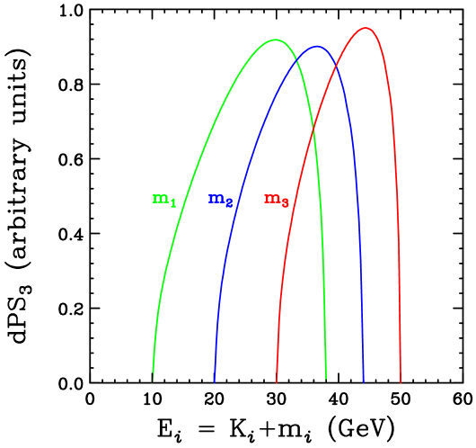
To see the non-monochromaticity of the energies in three-body kinematics, in Fig. 14, we plot the three-body phase space weight $dPS3$ as a function of $E_{i}\ (i=1,2,3)$. For definiteness, we choose $\sqrt{s}=100$ GeV and $m_{1,2,3}=10,\ 20,\ 30$ GeV, respectively. It is in arbitrary units, but scaled to dimensionless by dividing $E_{i}^{max}\sqrt{s}$. We see broad spectra for energy distributions. Naturally, the more massive a particle is, the more energetic (energy and momentum) it is, but narrower for the energy spread. However, its kinetic energy $K_{i}=E_{i}-m_{i}$ is smaller for larger $m_{i}$.

A.5 Recursion Relation for the Phase Space Element

$$dPS_{n}(P;p_{1},...,p_{n}) = dPS_{n-1}(P;p_{1},...,p_{n-1,n})$$ (99)

$$dPS_{2}(p_{n-1,n};p_{n-1},p_{n}){dm^{2}_{n-1,n}\over 2\pi}.$$

This recursion relation is particularly useful when we can write the intermediate mass integral for a resonant state.

Figure 15: Illustration for the recursion relation for an $n$-body kinematics.

Appendix B Breit-Wigner Resonance and the Narrow Width Approximation

The propagator contribution of an unstable particle of mass $M$ and total width $\Gamma_{V}$ is written as

$$R(s)=\frac{1}{(s-M^{2}_{V})^{2}+\Gamma_{V}^{2}M_{V}^{2}},$$ (100)

This is the Breit-Wigner Resonance.

Consider a very general case of a virtual particle $V^{*}$ in an intermediate state,

$$a\to bV^{*}\to b\ p_{1}p_{2}.$$ (101)

An integral over the virtual mass can be obtained by the reduction formula in the last section. Together with kinematical considerations, the resonant integral reads

$$\int_{(m^{min}_{*})^{2}=(m_{1}+m_{2})^{2}}^{(m^{max}_{*})^{2}=(m_{a}-m_{b})^{2}}{dm_{*}^{2}}.$$ (102)

The integral is rather singular near the resonance. Thus a variable change is effective for the practical purpose,

$$\tan\theta={{m_{*}^{2}-M_{V}^{2}}\over{\Gamma_{V}M_{V}}},$$ (103)

resulting in a flat integrand over $\theta$

$$\int_{(m^{min}_{*})^{2}}^{(m^{max}_{*})^{2}}\frac{dm_{*}^{2}}{(m^{2}_{*}-M^{2}_{V})^{2}+\Gamma_{V}^{2}M_{V}^{2}}=\int_{\theta^{min}}^{\theta^{max}}\frac{d\theta}{\Gamma_{V}M_{V}},$$ (104)

where $\theta=\tan^{-1}(m_{*}^{2}-M_{V}^{2})/\Gamma_{V}M_{V}$. In the limit

$$(m_{1}+m_{2})+\Gamma_{V}\ll M_{V}\ll m_{a}-\Gamma_{V},$$ (105)

then $\theta^{min}\to-\pi,\ \theta^{max}\to 0$. This is the condition for the narrow-width approximation:

$$\frac{1}{(m^{2}_{*}-M^{2}_{V})^{2}+\Gamma_{V}^{2}M_{V}^{2}}\approx\frac{\pi}{\Gamma_{V}M_{V}}\ \delta(m^{2}_{*}-M^{2}_{V}).$$ (106)

Exercise: Consider a three-body decay of a top quark, $t\to bW^{*}\to b\ e\nu.$ Making use of the phase space recursion relation and the narrow width approximation for the intermediate $W$ boson, show that the partial decay width of the top quark can be expressed as

$$\Gamma(t\to bW^{*}\to b\ e\nu)\approx\Gamma(t\to bW)\cdot BR(W\to e\nu).$$ (107)

References

- (1) S. Willenbrock, Symmetries of the Standard Model, these TASI lectures, arXiv:hep-ph/0410370, and references therein.
- (2) C. Quigg, Gauge Theories of the Strong, Weak, and Electromagnetic Interactions, Addison-Wesley Publishing Company, Inc. (1983); T.-P. Cheng and L.-F. Li, Gauge Theory of Elementary Particle Physics, Oxford University press (1984); J. Donoghue, E. Golowich, B.R. Holstein, Dynamics of the Standard Model, Cambridge University Press (1992).
- (3) H. Haber, Practical Supersymmetry, these TASI lectures. Also see his review in Reference PDG .
- (4) Particle Data Group, Review of Particle Physics, Phys. Lett. B592, 1 (2004).
- (5) M. Drees, R. M. Godbole, and Theory and Phenomenology of Sparticles, World Scientific Publisher (2004).
- (6) R. Sundrum, Introduction to Extra Dimensions, these TASI lectures.
- (7) C. Csaki, Higgsless Electroweak Symmetry Breaking, these TASI lectures. Also, see his previous TASI lectures, arXiv:hep-ph/0404096.
- (8) H. Schellman, these TASI lectures.
- (9) V.D. Barger and R.J.N. Phillips, Collider Physics, Addision-Wesley Publishing Company (1987).
- (10) R.K. Ellis, W.J. Stirling, and B.R. Webber, QCD and Collider Physics, Cambridge University Press (1996).
- (11) R. Fernow, Introduction to Experimental Particle Physics, Cambridge University Press (1990).
- (12) ATLAS Technical Design Report, CERN-LHCC-94-43.
- (13) CMS Technical Design Report, CERN-LHCC-94-38.
- (14) J.A. Aguilar-Saavedra et al., ECFA/DESY LC Physics Working Group Collaboration, DESY 2001-011 and arXiv:hep-ph/0106315; T. Abe et al., American LC Working Group Collaboration, arXiv:hep-ex/0106055; K. Abe et al., ACFA LC Working Group Collaboration, arXiv:hep-ex/0109166.
- (15) CLIC Working Group, Physics at the CLIC Multi-TeV Linear Collider, arXiv:hep-ph/0412251.
- (16) M. Blaskiewicz et al.. VLHC Accelerator Physics, FERMILAB-TM-2158.
- (17) V.D. Barger, M.S. Berger, J.F. Gunion, and T. Han, Phys. Rept. 286, 1 (1997).
- (18) I.F. Ginzburg, G.L. Kotkin, S.L. Panfil, V.G. Serbo, and V.I. Telnov, Nucl. Instr. and Methods in Phys. Res. 219, 5 (1984).
- (19) S. Dawson, Nucl. Phys. B249, 42 (1985); M. Chanowitz and M.K. Gailard, Phys. Lett. B142, 85 (1984).
- (20) G. Kane, W.W. Repko, and W.B. Rolnick, Phys. Lett. B148, 367 (1984).
- (21) K. Hagawara and D. Zeppenfeld, Nucl. Phys. B313, 560 (1989).
- (22) G. Moortgat-Pick et al.. arXiv:hep-ph/0507011.
- (23) G. Sterman, QCD and Jets, these TASI lectures. arxive:hep-ph/0412013.
- (24) H. L. Lai et al. [CTEQ Collaboration], Eur. Phys. J. C12, 375 (2000).
- (25) H. Cheng and T.T. Wu, Phys. Rev. Lett. 24, 1456 (1970).
- (26) E. Laenen, J. Smith, and W.L. van Neerven, Phys. Lett. B321, 254 (1994); E.L. Berger and H. Contopanagos, Phys. Lett. B361, 115 (1995); S. Catani, M.L. Mangano, P. Nason, and L. Trentadue, Phys. Lett. B378, 329 (1996).
- (27) R.V. Harlander and W.B. Kilgore, Phys. Rev. Lett. 88, 201801 (2002); C. Anastasiou and K. Melnikov, Nucl. Phys. B646, 220 (2002).
- (28) T. Han, G. Valencia, and S. Willenbrock, Phys. Rev. Lett. 69, 3274 (1992); T. Figy, C. Oleari, and D. Zeppenfeld, Phys. Rev. D68, 073005 (2003); E.L. Berger and J. Campbell, Phys. Rev. D70, 073011 (2004).
- (29) K.T. Pitts for the CDF and D0 Collaborations, arXiv:hep-ex/0102010.
- (30) V. Barger, A.D. Martin, and R.J.N. Phillips, Z. Phys. C21, 99 (1983).
- (31) D. Acosta et al., CDF II Collaboration, Phys. Rev. Lett. 94, 091803 (2005).
- (32) V. Barger, T. Han, and R.J. Phillips, Phys. Rev. D36, 295 (1987); ibid., D37, 2005 (1988).
- (33) V. Barger, T. Han, and J. Ohnemus, Phys. Rev. D37, 1174 (1988).
- (34) M. Dittmar and H. K. Dreiner, Phys. Rev. D55, 167 (1997).
- (35) T. Han and R.-J. Zhang, Phys. Rev. Lett. 82, 25 (1999); T. Han, A. S. Turcot, and R.-J. Zhang, Phys. Rev. D59, 093001 (1999).
- (36) R.N. Cahn,, S.D. Ellis, R. Kleiss, and W.James Stirling, Phys.Rev. D35, 1626 (1987); V.D. Barger, T. Han, and R.J.N. Phillips, Phys. Rev. D37, 2005 (1988); R. Kleiss and W.James Stirling, Phys.Lett. B200, 193 (1988).
- (37) V. Barger, K. Cheung, T. Han, and R.J. Phillips, Phys. Rev. D42, 3052 (1990).
- (38) J. Bagger, V. Barger, K. Cheung, J. Gunion, T. Han, G. Ladinsky, R. Rosenfeld, and C.-P. Yuan, Phys. Rev. D49, 1246 (1994); ibid, D52, 3878 (1995).
- (39) V. Barger, R.J.N. Phillips, and D. Zeppenfeld, Phys. Lett. B346, 106 (1995); D. Rainwater, D. Zeppenfeld, and K. Hagiwara, Phys. Rev. D59, 014037 (1999).
- (40) P. Langacker, R. W. Robinett and J. L. Rosner, Phys. Rev. D30, 1470 (1984); V. D. Barger, N. G. Deshpande, J. L. Rosner and K. Whisnant, Phys. Rev. D35, 2893 (1987); J. L. Rosner, Phys. Rev. D54, 1078 (1996).
- (41) T. Han, H.E. Logan, and L.-T. Wang, arXiv:hep-ph/0506313.
- (42) J. L. Hewett and T. G. Rizzo, Phys. Rept. 183, 193 (1989); M. Cvetic and P. Langacker, Phys. Rev. D42, 1797 (1990).
- (43) G. Burdman, M. Perelstein and A. Pierce, Phys. Rev. Lett. 90, 241802 (2003) [Erratum-ibid. 92, 049903 (2004)].
- (44) T. Han, H. E. Logan, B. McElrath and L. T. Wang, Phys. Rev. D67, 095004 (2003).
- (45) E. Eichten, K. D. Lane and J. Womersley, Phys. Lett. B405, 305 (1997).
- (46) H. Davoudiasl, J. L. Hewett and T. G. Rizzo, Phys. Rev. D63, 075004 (2001); B. C. Allanach, K. Odagiri, M. J. Palmer, M. A. Parker, A. Sabetfakhri and B. R. Webber, JHEP 0212, 039 (2002).
- (47) H. K. Dreiner and G. G. Ross, Nucl. Phys. B365, 597 (1991); E. L. Berger, B. W. Harris and Z. Sullivan, Phys. Rev. Lett. 83, 4472 (1999); T. Plehn, Phys. Lett. B488, 359 (2000).
- (48) D. Choudhury, A. Datta, K. Huitu, P. Konar, S. Moretti and B. Mukhopadhyaya, Phys. Rev. D68, 075007 (2003); P. Konar and B. Mukhopadhyaya, Phys. Rev. D70, 115011 (2004).
- (49) R. Vega and D. A. Dicus, Nucl. Phys. B329, 533 (1990).
- (50) M. Perelstein, M. E. Peskin and A. Pierce, Phys. Rev. D69, 075002 (2004).
- (51) H. Baer, X. Tata, and J. Woodside, Phys. Rev. Lett. 63, 352 (1989).
- (52) H.E. Haber and G.L. Kane, Phys. Rept. 117, 75 (1985).
- (53) G. F. Giudice, R. Rattazzi and J. D. Wells, Nucl. Phys. B544, 3 (1999); T. Han, J. D. Lykken and R. J. Zhang, Phys. Rev. D59, 105006 (1999); E. A. Mirabelli, M. Perelstein and M. E. Peskin, Phys. Rev. Lett. 82, 2236 (1999).
- (54) T. Appelquist, H. C. Cheng and B. A. Dobrescu, Phys. Rev. D64, 035002 (2001); H. C. Cheng, K. T. Matchev and M. Schmaltz, Phys. Rev. D66, 056006 (2002).
- (55) H. C. Cheng and I. Low, JHEP 0309, 051 (2003); J. Hubisz and P. Meade, Phys. Rev. D71, 035016 (2005).
- (56) I. Hinchliffe and F. E. Paige, Phys. Rev. D60, 095002 (1999); H. Bachacou, I. Hinchliffe and F. E. Paige, Phys. Rev. D62, 015009 (2000); K. Kawagoe, M. M. Nojiri and G. Polesello, Phys. Rev. D71, 035008 (2005).