Factorization in exclusive semileptonic radiative $B$ decays

Abstract

We derive a new factorization relation for the semileptonic radiative decay $B\to\pi\ell\nu\gamma$ in the kinematical region of a slow pion $|\vec{p}_{\pi}\,|\sim\Lambda$ and an energetic photon $E_{\gamma}\gg\Lambda$, working at leading order in $\Lambda/m_{b}$. In the limit of a soft pion, the nonperturbative matrix element appearing in this relation can be computed using chiral perturbation theory. We present a phenomenological study of this decay, which may be important for a precise determination of the exclusive nonradiative decay.

I Introduction

Experiments at the B factories are reaching an accuracy level that requires a good understanding of radiative effects in weak B decays. In particular, real photon emission distorts the spectra of other decay products, therefore directly affecting the distribution of kinematic quantities used to select and count signal events RadCorr ; CGatti . As a consequence, real photon emission indirectly affects branching fraction measurements, leading to systematic shifts of the order of a few percent. While radiative effects are well studied in semileptonic and nonleptonic kaon decays, where chiral perturbation theory is applicable over the entire kinematical range (see Refs. kl31 ; kl32 ; D'Ambrosio:1994ae ), the situation is less satisfactory in B decays. Here the large energy release generally prohibits the application of chiral perturbation theory methods over large parts of the phase space, and one has to resort to different theoretical tools.

We study here one of the simplest radiative processes, the semileptonic radiative B decays $B\to\pi\ell\nu\gamma$. The corresponding nonradiative process, the semileptonic decay $B\to\pi\ell\nu$, is well studied in connection with the determination of the CKM matrix element $|V_{ub}|$. The measured branching fractions of this mode are exp

$${\cal B}(B^{0}\to\pi^{-}\ell^{+}\nu)=$$ (1)

$$\left\{\begin{array}[]{cc}(1.33\pm 0.18\pm 0.13)\times 10^{-4}&\mbox{(CLEO)}\\ (1.38\pm 0.10\pm 0.18)\times 10^{-4}&\mbox{(BABAR)}\\ (1.48\pm 0.20\pm 0.16)\times 10^{-4}&\mbox{(BELLE)}\\ \end{array}\right.$$ (5)

which contribute to the world average $B(B^{0}\to\pi^{-}\ell^{+}\nu)=(1.35\pm 0.08\pm 0.08)\times 10^{-4}$ hfag .

The hadronic dynamics of the radiative semileptonic decays is complicated by the presence of many energy scales. However, in certain kinematical regions a model independent treatment is possible. In the limit of a soft photon, Low’s theorem Low fixes the terms of order $O(q^{-1})$ and $O(q^{0})$ in the expansion of the decay amplitude in powers of the photon momentum $q$. These contributions have been computed in fearing in kaon semileptonic radiative decays $K_{\ell 3}$. Higher order terms in $q$ have been more recently obtained using chiral perturbation theory kl31 ; kl32 . A similar approach is possible in B decays with the help of the heavy hadron chiral perturbation theory wise ; BuDo ; TM ; review , as long as the pion and photon are sufficiently soft. This is the case in a limited corner of the phase space, corresponding to a large dilepton invariant mass $W^{2}=(p_{e}+p_{\nu})^{2}\sim m_{b}^{2}$.

The radiative semileptonic decay $B\to\gamma\pi\ell\bar{\nu}_{\ell}$ at low $W^{2}$ produces in general either an energetic pion or an energetic photon (see Fig. 1). In this paper we use soft-collinear effective theory (SCET) scet0 ; bfps ; scet2 ; scet3 -scet3.5 ; scet4 methods to prove a factorization relation for the decay amplitude in the kinematical region with an energetic photon and a soft pion. This can be written schematically as

$$A(B\to\pi\ell\nu\gamma)=H\otimes J\otimes S(B\to\pi)+O(\Lambda/Q)$$ (6)

with $\Lambda\sim\Lambda_{QCD}$ and $Q\sim\{E_{\gamma},m_{b}\}$. Here $H$ and $J$ are hard and jet functions, calculable in perturbation theory. $S(B\to\pi)$ is related to the matrix element of a nonlocal soft operator which describes the $B\to\pi$ transition. This factorization relation generalizes to any process $B\to\gamma M\ell\nu$ ($M=\rho,\omega,\cdots$ a light soft meson) with the appropriate soft function $S(B\to M)$ replacing $S(B\to\pi)$. In this work we use heavy hadron chiral perturbation theory to compute the soft matrix element $S(B\to\pi)$, and express it in terms of one of the B meson light-cone wave functions $\phi_{+}^{B}(k_{+})$ GPchiral . The convolution of this function with the jet function $J$ in Eq. (6) is similar to the one appearing in a factorization relation for the radiative leptonic decay $B\to\gamma\ell\nu$ radlept0 ; radlept1 ; radlept2 ; radlept3 .

The paper is organized as follows: after fixing the notation in Section II, we describe the main results of the paper (factorization formula for hadronic form factors) in Section III. We give a proof of the factorization formula in Section IV. In Section V we explore the phenomenological consequences of our results, computing the radiative branching fractions with appropriate cuts on the photon and pion energy, as well as various differential decay distributions. The factorization results are compared with the ones obtained by extrapolating Low’s amplitude to the region of an energetic photon. We collect our conclusions in Section VI. An appendix contains the expression of the radiative amplitude in Low’s limit of a soft photon.

II Amplitude definitions

We consider in this paper the radiative semileptonic B decays

$$\bar{B}(p)\to\pi(p^{\prime})\,e^{-}(p_{e})\,\bar{\nu}(p_{\nu})\,\gamma(q,\varepsilon)\ ,$$ (7)

mediated by the combined semileptonic weak Hamiltonian

$${\cal H}_{W}=\frac{4G_{F}}{\sqrt{2}}V_{ub}[\bar{u}\gamma_{\mu}P_{L}b][\bar{e}\gamma^{\mu}P_{L}\nu]$$ (8)

and the electromagnetic coupling of quarks and charged leptons.

The full amplitude for $\bar{B}(p)\to\pi(p^{\prime})e^{-}(p_{e})\bar{\nu}(p_{\nu})\gamma(q,\varepsilon)$ contains two terms, describing the photon coupling to the hadronic system and to the charged lepton, respectively

$$A = \frac{eG_{F}}{\sqrt{2}}V_{ub}\varepsilon^{\mu}(q)^{*}\Big{[}\left(T_{\mu\nu}^{V}-T_{\mu\nu}^{A}\right)\,\bar{u}(p_{e})\gamma^{\nu}(1-\gamma_{5})v(p_{\nu})$$

$$+ \frac{F^{\nu}(p,p^{\prime})}{2\,q\cdot p_{e}}\,\bar{u}(p_{e})\gamma_{\mu}(m_{e}+p_{e}/+q/)\gamma_{\nu}(1-\gamma_{5})v(p_{\nu})\Big{]}\ .$$

We denoted here

$$F_{\nu}(p,p^{\prime})=\langle\pi(p^{\prime})|\bar{u}\gamma_{\nu}b|\bar{B}(p)\rangle\ ,$$ (10)

and the hadronic tensors $T_{\mu\nu}^{V,A}$ are defined as

$$T^{J}_{\mu\nu}=i\int d^{4}xe^{iq\cdot x}\langle\pi(p^{\prime})|\mbox{T}\left\{j_{\mu}^{\rm em}(x)\,,J_{\nu}(0)\right\}|\bar{B}(p)\rangle$$ (11)

with $j_{\mu}^{\rm em}=\sum_{q}e_{q}\bar{q}\gamma_{\mu}q$ the quarks’ electromagnetic current and:

$$T^{V}_{\mu\nu}\,:\qquad J_{\nu}=V_{\nu}=\bar{u}\gamma_{\nu}b$$ (12)

$$T^{A}_{\mu\nu}\,:\qquad J_{\nu}=A_{\nu}=\bar{u}\gamma_{\nu}\gamma_{5}b\,.$$ (13)

The hadronic tensors satisfy the Ward identities

$$q^{\mu}T^{V}_{\mu\nu}=-F_{\nu}(p,p^{\prime})$$ (14)

$$q^{\mu}T^{A}_{\mu\nu}=0\ .$$ (15)

The most general form for the vector amplitude compatible with the Ward identity can be written in terms of 4 invariants $V_{1-4}$. After multiplication with the photon polarization, this is written as ($W=p_{e}+p_{\nu}$)

$$\varepsilon^{*\mu}T^{V}_{\mu\nu}=V_{1}(\varepsilon_{\nu}^{*}-\frac{\varepsilon^{*}\cdot W}{q\cdot W}q_{\nu})$$ (16)

$$+(p^{\prime}\cdot\varepsilon^{*}-\frac{(p^{\prime}\cdot q)(\varepsilon^{*}\cdot W)}{q\cdot W})(V_{2}q_{\nu}+V_{3}W_{\nu}+V_{4}p^{\prime}_{\nu})$$

$$\qquad-\frac{\varepsilon^{*}\cdot W}{q\cdot W}F_{\nu}(p,p^{\prime})\,.$$

The axial amplitude $T^{A}_{\mu\nu}$ can be written in terms of another four invariants $A_{1-4}$. They can be chosen as

$$\varepsilon^{*\mu}T^{A}_{\mu\nu} = i\epsilon_{\mu\nu\rho\sigma}\varepsilon^{*\mu}(A_{1}p^{\prime}_{\rho}q_{\sigma}+A_{2}q_{\rho}W_{\sigma})$$

$$+ i\epsilon_{\mu\lambda\rho\sigma}\varepsilon^{*\mu}p^{\prime}_{\lambda}q_{\rho}W_{\sigma}(A_{3}W_{\nu}+A_{4}p^{\prime}_{\nu})$$

The invariant form factors $V_{1-4}$ and $A_{1-4}$ depend on 3 independent kinematical variables, which can be chosen as $W^{2},E_{\pi},E_{\gamma}$ with $E_{\pi}$ and $E_{\gamma}$ defined as the pion and photon energy in the rest frame of the B meson. For given $W^{2}$, the possible final states in the decay can be represented as points in the Dalitz plot for $(E_{\gamma},E_{\pi})$. We show in Fig. 1 the Dalitz plot for $W^{2}=4$ GeV². The dilepton invariant mass $W^{2}$ can take values $W^{2}=[0,(m_{B}-m_{\pi})^{2}]=[0,26.5]$ GeV².

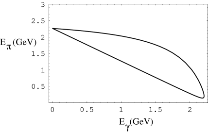
Figure 1: The Dalitz plot for $B\to\gamma\pi\ell\bar{\nu}$ at $W^{2}=4$ GeV². Our computation of the form factors is applicable in the lower right corner of the Dalitz plot, with an energetic photon and a soft pion.

The form factors in $B$ (quark content $\bar{b}q$) and $\bar{B}$ ($b\bar{q}$ quark content) are related by charge conjugation. The transformations of the currents under charge conjugation are

$${\cal C}\bar{q}\gamma_{\nu}b{\cal C}^{\dagger}=-\bar{b}\gamma_{\nu}q\,,\quad{\cal C}\bar{q}\gamma_{\nu}\gamma_{5}b{\cal C}^{\dagger}=\bar{b}\gamma_{\nu}\gamma_{5}q$$ (18)

We adopt everywhere in this paper the following phase conventions for the meson states

$$(\pi^{+}\,,\pi^{0}\,,\pi^{-})=(u\bar{d},\frac{1}{\sqrt{2}}(u\bar{u}-d\bar{d}),d\bar{u})$$ (19)

$$(B^{-},\bar{B}^{0})=(b\bar{u},b\bar{d})\,,\quad(B^{0},B^{+})=(\bar{b}d,\bar{b}u)\,.$$ (20)

With this convention the states transform as ${\cal C}\pi^{+}=\pi^{-}\,,{\cal C}\bar{B}^{0}=B^{0}\,,{\cal C}B^{-}=B^{+}$. In addition, the $\pi^{0}$ is C-even and the photon is C-odd. The semileptonic radiative $B\to\pi$ form factors transform as follows under charge conjugation, independent of the flavor of the spectator quark

$$V_{1-4}(\bar{B}\to\pi\gamma\ell^{-}\bar{\nu}_{\ell})=V_{1-4}(B\to\pi\gamma\ell^{+}\nu_{\ell})$$ (22)

$$A_{1-4}(\bar{B}\to\pi\gamma\ell^{-}\bar{\nu}_{\ell})=-A_{1-4}(B\to\pi\gamma\ell^{+}\nu_{\ell})$$

The vector form factor $F_{\nu}(p,p^{\prime})$ is C-odd. Finally, the form factors depend also on the flavor of the light spectator in the B meson. For simplicity of notation, we chose to omit this dependence, but it will be specified explicitly whenever required.

III Results

We describe here the main results of this paper. In the kinematical region $E_{\gamma}\gg\Lambda$ and $E_{\pi}\sim\Lambda$ (hard photon and soft pion), the form factors for $B\to\pi\ell\nu\gamma$ are given by a factorization theorem. At leading order in $\Lambda/Q$ with $Q\sim\{m_{b},E_{\gamma}\}$, these factorization relations are the same for both $B^{-},\bar{B}^{0}$, up to an isospin factor. The predictions for the vector form factors in $\bar{B}^{0}\to\pi^{+}\ell^{-}\bar{\nu}\gamma$ are

$$V_{1}=2e_{u}C_{1}^{(v)}(E_{\gamma})\int dk_{+}J(k_{+})S_{1}(k_{+},t^{2},\zeta)$$ (23)

$$V_{2}=\frac{e_{u}}{E_{\gamma}}\Big{(}2C_{1}^{(v)}(E_{\gamma})+C_{2}^{(v)}(E_{\gamma})+2C_{3}^{(v)}(E_{\gamma})\Big{)}$$

$$\qquad\qquad\times\int dk_{+}J(k_{+})S_{2}(k_{+},t^{2},\zeta)$$ (24)

$$V_{3}=\frac{2e_{u}}{n\cdot W}C_{2}^{(v)}(E_{\gamma})\int dk_{+}J(k_{+})S_{2}(k_{+},t^{2},\zeta)$$ (25)

$$V_{4}/V_{1}\sim O(\frac{1}{\Lambda Q})$$ (26)

and the corresponding relations for the axial form factors are

$$A_{1}=\frac{e_{u}}{E_{\gamma}}\Big{(}2C_{1}^{(v)}(E_{\gamma})+C_{2}^{(v)}(E_{\gamma})+2C_{3}^{(v)}(E_{\gamma})\Big{)}$$

$$\qquad\qquad\times\int dk_{+}J(k_{+})S_{2}(k_{+},t^{2},\zeta)$$ (27)

$$A_{2}=\frac{2e_{u}}{q\cdot W}C_{1}^{(v)}(E_{\gamma})\int dk_{+}J(k_{+})S_{1}(k_{+},t^{2},\zeta)$$ (28)

$$A_{3}=\frac{2e_{u}}{q\cdot Wn\cdot W}C_{2}^{(v)}(E_{\gamma})$$ (29)

$$\qquad\qquad\times\int dk_{+}J(k_{+})S_{2}(k_{+},t^{2},\zeta)$$

$$A_{4}/A_{2}\sim O(\frac{1}{\Lambda Q})\,.$$ (30)

After multiplication by the appropriate tensor structures, $V_{4}$ and $A_{4}$ give subleading contributions in $\Lambda/Q$ to the hadronic tensor. The corresponding form factors for $B^{-}\to\gamma\pi^{0}\ell^{-}\bar{\nu}$ are multiplied by a factor $1/\sqrt{2}$. In these formulas $n_{\mu}=q_{\mu}/E_{\gamma}$ is a light-cone unit vector along the photon momentum.

The hard functions $C_{1-3}^{(v)}(E_{\gamma})$ are Wilson coefficients in the SCET, and are calculable in perturbation theory in an expansion in $\alpha_{s}(Q)$ as $C_{1}^{(v)}=1+O(\alpha_{s}(m_{b}))\,,C_{2,3}^{(v)}=O(\alpha_{s}(m_{b}))$. Their one-loop expressions can be found in Ref. bfps . The jet function $J(k_{+})$ is calculable in an expansion of $\alpha_{s}(\sqrt{Q\Lambda})$ and its one-loop expression is given below in Eq. (40). Finally, $S_{1,2}(k_{+},t^{2},\zeta)$ are nonperturbative soft matrix elements, defined below in Eqs. (42), (43).

The results (23)-(30) show that, at leading order in $\Lambda/Q$, the eight form factors parameterizing $B\to\gamma\pi e\nu$ are given by only two nonperturbative parameters and thus satisfy symmetry relations.

The soft functions $S_{1,2}$ depend in general on $k_{+}$, $t^{2}=(p-p^{\prime})^{2}$, $\zeta=n\cdot p^{\prime}/n\cdot p$, and are calculable at leading order in chiral perturbation theory. In the soft pion limit they can be expressed in terms of one of the $B$ meson light-cone wave function and are given by

$$S_{1}(k_{+},t^{2},\zeta) = -\frac{f_{B}m_{B}}{4f_{\pi}}\phi_{+}^{B}(k_{+})\left(1+g\frac{e_{3}\cdot p^{\prime}}{v\cdot p^{\prime}+\Delta}\right)\ \ \ \$$ (31)

$$S_{2}(k_{+},t^{2},\zeta) = \frac{gf_{B}m_{B}}{4f_{\pi}}\phi_{+}^{B}(k_{+})\frac{1}{v\cdot p^{\prime}+\Delta}$$ (32)

where $v=p/m_{B}$, $\Delta=m_{B^{*}}-m_{B}=50$ MeV, $e_{3}=n-v$, and $g$ is the axial effective coupling defined in Eq. (52). To this order, the dependence on nonperturbative dynamics of the B meson enters only through one quantity, the convolution of the light-cone B wave function $\phi_{+}^{B}(k_{+})$ with the jet function $J(k_{+})$:

$$V_{i}\,,\,A_{i}\ \propto\int dk_{+}J(k_{+})\phi_{B}^{+}(k_{+},\mu)\ .$$ (33)

A similar convolution appears in the factorization relation for the radiative leptonic $B$ decay $B\to\gamma e\bar{\nu}$, the only difference being that in this case the argument of the jet function is time-like ($+2E_{\gamma}k_{+}$) as opposed to spacelike in the radiative leptonic case. As a consequence the form factors $V_{i}$ and $A_{i}$ are in general complex, receiving strong phases of $\sim\alpha_{s}(\sqrt{2E_{\gamma}\Lambda})$ via the loop corrections to the jet function $J$.

IV Factorization proof

The proof of the relations Eqs. (23)-(30) makes use of the soft collinear effective theory (SCET) scet0 ; bfps ; scet2 ; scet3 ; scet3.5 ; scet4 . The basic idea will be to match the correlator of currents in Eq. (11) onto soft SCET operators, and then in a second step to construct the chiral representation of the resulting soft operators. The $B\to\pi$ matrix element of the correlator in Eq. (11) will be computed in the low energy chiral perturbation theory.

We start by setting up the kinematics of the process. We introduce two light cone unit vectors $n,\bar{n}$ with $n^{2}=\bar{n}^{2}=0\,,n\cdot\bar{n}=2$. The dilepton momentum $W$ is chosen along $\bar{n}$ with light cone coordinates $W=(n\cdot W,\bar{n}\cdot W,W_{\perp})$ (such that $n\cdot W\gg\bar{n}\cdot W,W_{\perp}$). The photon is emitted along $n_{\mu}$, such that its light-cone coordinates are $q=(0,\bar{n}\cdot q,0)$, and the pion momentum is soft, with components $p_{\pi}\sim\Lambda$.

We are interested in the correlator of the weak semileptonic current with the electromagnetic current

$$T_{\mu\nu}(q)=i\int d^{4}xe^{iq.x}T\{(\bar{q}\gamma_{\nu}P_{L}b)(0)\,,j_{\mu}^{\rm e.m.}(x)\}$$ (34)

The matrix elements of this correlator define the hadronic tensors in the decays of interest Eqs. (11). The flavor dependence of the form factors follows from the transformation properties of this correlator under flavor SU(3). This is given by $\overline{\mathbf{3}}\otimes{\mathbf{8}}=\overline{\mathbf{3}}+{\mathbf{6}}+\overline{\mathbf{1}5}$, so that the $\bar{B}\to\pi$ transitions are in general described by three unknown reduced matrix elements. However, at leading order in $\Lambda/E_{\gamma}$, only one amplitude contributes. To see this, consider the two types of contributions to the correlator $T_{\mu\nu}(q)$, corresponding to the photon attaching either to the current quarks ($u$ and $b$), or the spectator quark. At leading order in $\Lambda/E_{\gamma}$, only the first amplitude contributes, while the spectator effect is power suppressed (see below). The dominant amplitudes transform as a $\overline{\mathbf{3}}$ under flavor SU(3), so they are independent of the flavor of the spectator quark.

The semileptonic $b\to u$ current is first matched onto SCET_I, an effective theory containing ultrasoft quarks and gluons with momenta $p_{s}\sim\Lambda$, and collinear modes with virtuality $p_{c}^{2}\sim Q\Lambda$ moving along $q_{\mu}\sim n_{\mu}$ bfps . Neglecting light quark masses, the $V-A$ current is matched at leading order in $\lambda\equiv\Lambda/Q$ only onto structures containing one left-handed light quark field bfps

$$\bar{q}\gamma_{\mu}P_{L}b=C_{1}^{(v)}(\omega)\bar{q}_{n,\omega}\gamma_{\mu}P_{L}b_{v}$$ (35)

$$+(C_{2}^{(v)}(\omega)v_{\mu}+C_{3}^{(v)}(\omega)\frac{n_{\mu}}{n\cdot v})\bar{q}_{n,\omega}P_{R}b_{v}+O(\lambda)$$

where $C_{i}^{(v)}(\omega)$ are Wilson coefficients calculable in perturbation theory as an expansion in $\alpha_{s}(Q)$.

We match first the correlator Eq. (34) onto SCET_I operators. The weak current is matched as shown above in Eq. (35). The light quark e.m. current coupling $\bar{q}{\cal A}_{n}\xi_{n}$ of an energetic ($n-$collinear) photon to a ultrasoft quark is more complicated, and it contains both a local and a nonlocal term radlept2

$$\varepsilon^{*\mu}j_{\mu}^{\rm e.m.}=e_{q}\,\bar{q}\varepsilon/^{*}q_{n,\omega}+T\{J^{\xi\xi}\,,\int d^{4}xi{\cal L}_{q\xi}^{(1)}(x)\}$$ (36)

where $J^{\xi\xi}$ describes the coupling of a $n-$collinear photon to $n-$collinear quarks. This scales like $O(\lambda^{-1})$ and it appears in time-ordered products with a subleading ultrasoft-collinear Lagrangian. It is given by

$$J^{\xi\xi} = e_{q}\,\bar{q}_{n,\omega_{1}}\varepsilon/^{*}\frac{1}{\bar{n}\cdot i\partial}\big{[}W^{\dagger}iD/_{c\perp}\frac{\bar{n}\!\!\!/}{2}\xi_{n}\big{]}_{\omega_{2}}$$

$$+e_{q}\,\big{[}\bar{\xi}_{n}iD/_{c\perp}W\big{]}_{\omega_{1}}\frac{1}{\bar{n}\cdot i\partial}\varepsilon/^{*}\frac{\bar{n}\!\!\!/}{2}q_{n,\omega_{2}}$$

Finally, we match the SCET_I expression of the correlator (34) onto SCET_II. After soft-collinear factorization scet3 , the collinear quarks and gluons with virtuality $p_{c}^{2}\sim E_{\gamma}\Lambda$ decouple from the soft modes. This leads to the final form of the time-ordered product in Eq. (34) in the effective theory

$$\varepsilon^{*\mu}T_{\mu\nu}(q)\to-C_{1}^{(v)}\,e_{u}\,\int dk_{+}J(k_{+})O_{1\nu}(k_{+})$$

$$\!-\![C_{2}^{(v)}v_{\nu}+(C_{1}^{(v)}\!+C_{3}^{(v)})\frac{n_{\nu}}{n\cdot v}]e_{u}\!\!\int\!dk_{+}J(k_{+})O_{2}(k_{+})\ ,$$

with the two soft operators given by nonlocal quark bilinears

$$O_{1\mu}(k_{+}) = \int\frac{d\lambda}{4\pi}e^{-\frac{i}{2}\lambda k_{+}}\,\bar{q}(\lambda\frac{n}{2})Y_{n}(\lambda\frac{n}{2},0)\varepsilon/^{*}_{\perp}\frac{n\!\!\!/}{2}\gamma_{\mu}^{\perp}P_{L}b_{v}(0)$$

$$O_{2}(k_{+}) = \int\frac{d\lambda}{4\pi}e^{-\frac{i}{2}\lambda k_{+}}\,\bar{q}(\lambda\frac{n}{2})Y_{n}(\lambda\frac{n}{2},0)\varepsilon/^{*}_{\perp}\frac{n\!\!\!/}{2}P_{R}b_{v}(0)\ .$$

Here $Y_{n}(x,y)=P\exp(ig\int_{y_{-}}^{x_{-}}d\alpha\,n\cdot A(\alpha n))$ is a Wilson line along $n_{\mu}$.

The jet function $J$ describes the effects of the collinear quarks and gluons with virtualities $p_{c}^{2}\sim E_{\gamma}\Lambda$. It can be written as a vacuum expectation value of SCET_I collinear fields radlept2 , and as such it is calculable in perturbation theory in an expansion in $\alpha_{s}(\sqrt{Q\Lambda})$. The explicit result to subleading order in $\alpha_{s}$ is (with $L=\log[(-2E_{\gamma}k_{+}-i\varepsilon)/\mu^{2})$)

$$J(k_{+})=\frac{1}{k_{+}+i\varepsilon}\left(1+\frac{\alpha_{s}C_{F}}{4\pi}(L^{2}-1-\frac{\pi^{2}}{6})\right)$$ (40)

Finally, the nonperturbative physics is contained in the matrix elements of the soft operators $O_{1\mu}(k_{+})$ and $O_{2}(k_{+})$ in Eq. (LABEL:O12).

An alternative derivation is possible, wherein one matches directly from QCD onto SCET_II. In this approach radlept3 ; qcd2scet2 , the jet function $J$ together with the hard coefficients $C_{i}^{(v)}$ are obtained as the Wilson coefficient in the QCD $\to$ SCET_II matching. We will use here the 2-step approach, which has the advantage of allowing a transparent connection between the SCET_I Wilson coefficients in (35) and the Wilson coefficient of the SCET_II operator.

The discussion above parallels closely the proof of factorization in $B\to\gamma\ell\bar{\nu}$ decays in Ref. radlept2 , except that we were careful to keep it independent on the final hadronic state, which is only assumed to be soft. For example, we included also the operators in the second term of Eq. (IV) which do not contribute to leptonic radiative B decays.

To complete the proof of factorization one has to show that no other operators can appear at leading order in Eq. (IV). Since soft-collinear factorization in SCET_I preserves the form of the soft operators, it is clear that the T-products of the operators contributing to the weak current Eq. (35), and to the e.m. current Eq. (36), will always reduce to combinations of $O_{1\mu}$ and $O_{2}$. Photon couplings to the spectator quarks require at least 2 insertions of the soft-collinear Lagrangian ${\cal L}_{q\xi}^{(1)}$, so they are power suppressed. Finally, no operators containing additional soft quarks and gluons appear at leading order; the proof is similar to that for $B\to\gamma e\nu$, to which such operators would also contribute. For a recent study of these subleading contributions in the radiative leptonic decay, see Ref. subl .

Taking the $B\to$ vacuum matrix element of the SCET_II operators in Eq. (IV) gives directly the hadronic tensor relevant for the radiative leptonic $B\to\gamma\ell\nu$. This can be evaluated explicitly using the $B\to 0$ matrix element of the soft operator $O_{1\mu}(k_{+})$. The latter is parameterized in terms of the B meson light-cone wave functions, defined as radlept3

$$\int\frac{d\lambda}{4\pi}e^{-\frac{i}{2}k_{+}\lambda}\langle 0|\bar{q}_{i}(\lambda\frac{n}{2})Y_{n}(\lambda,0)b_{v}^{j}(0)|\bar{B}(v)\rangle=$$

$$-\frac{i}{4}f_{B}m_{B}\left\{\frac{1+v/}{2}[\bar{n}\!\!\!/n\cdot v\phi_{+}(k_{+})+n\!\!\!/\bar{n}\cdot v\phi_{-}(k_{+})]\gamma_{5}\right\}_{ji}$$

With this definition, the wave functions are normalized as $\int dk_{+}\phi_{\pm}(k_{+})=1$. Using the soft matrix element Eq. (IV) into Eq. (IV) reproduces the leading order factorization relation for the radiative leptonic decay form factors radlept0 ; radlept1 ; radlept2 ; radlept3 .

Proceeding in a similar way, by taking the matrix element of the operator identity Eq. (IV) for the $B\to\pi$ transition (with $\pi$ a soft pion) gives a factorization relation for the semileptonic radiative decay $B\to\pi\gamma e\bar{\nu}$. This requires the introduction of the soft functions $S_{1,2}(k_{+},t^{2},\zeta)$ defined by (with $t=p-p^{\prime}$ and $\zeta=(n\cdot p^{\prime})/(n\cdot v)$)

$$\langle\pi(p^{\prime})|O_{1\mu}(k_{+})|\bar{B}^{0}(v)\rangle$$ (42)

$$\hskip 56.9055pt=-(g_{\mu\nu}^{\perp}+i\varepsilon_{\mu\nu}^{\perp})\varepsilon^{*}_{\nu}S_{1}(k_{+},t^{2},\zeta)$$

$$\langle\pi(p^{\prime})|O_{2}(k_{+})|\bar{B}^{0}(v)\rangle$$ (43)

$$\hskip 56.9055pt=-(g_{\mu\nu}^{\perp}+i\varepsilon_{\mu\nu}^{\perp})\varepsilon^{*}_{\nu}p^{\prime}_{\mu}S_{2}(k_{+},t^{2},\zeta)\,,$$

Similar nonperturbative functions appear in the theory of off-diagonal hard-scattering exclusive processes GPD , and are known as GPDs (generalized parton distributions). See Refs. GPDreviews for recent reviews. In the context of $b\to u$ decays, they were considered previously in Ref. skewb , and $S_{1}$ is directly related to the function $\tilde{\cal F}_{\zeta}^{(1)}(x,q^{2})$ introduced in that paper.

The soft functions $S_{1,2}$ satisfy several model-independent constraints. T invariance and complex conjugation constrains them to be real. Their zeroth moments over $k_{+}$ are related to the usual $B\to\pi$ form factors (see the Appendix for the definitions of the form factors)

$$\int_{0}^{\infty}\mbox{d}k_{+}S_{1}(k_{+},t^{2},\zeta)=-\frac{1}{2}n\cdot pf_{+}(t^{2})+\frac{1}{4}f_{2}(t^{2})n\cdot t$$

$$\int_{0}^{\infty}\mbox{d}k_{+}S_{2}(k_{+},t^{2},\zeta)=\frac{1}{4}n\cdot pf_{T}(t^{2})\,.$$ (44)

while higher moments are related to the corresponding form factors of higher-dimensional operators

$$\int_{0}^{\infty}\mbox{d}k_{+}(k_{+})^{N}S_{1}(k_{+},t^{2},\zeta)$$ (45)

$$\qquad=-\langle\pi(p^{\prime})|\bar{q}(-n\cdot i{\overleftarrow{D}})^{N}\frac{n\!\!\!/}{2}P_{L}b_{v}|\bar{B}(p)\rangle$$

$$p^{\prime\perp}_{\nu}\int_{0}^{\infty}\mbox{d}k_{+}(k_{+})^{N}S_{2}(k_{+},t^{2},\zeta)$$ (46)

$$\qquad=-\frac{1}{2}\langle\pi(p^{\prime})|\bar{q}(-n\cdot i{\overleftarrow{D}})^{N}\frac{n\!\!\!/}{2}\gamma_{\nu}^{\perp}b_{v}|\bar{B}(p)\rangle$$

Inserting the definitions of the soft functions Eqs. (42), (43) into the operator expression for the hadronic tensor $T_{\mu\nu}$ Eq. (IV), one finds the leading order factorization relations listed in Eqs. (23)-(III).

Similar relations can be given for other semileptonic radiative B decays, such as $B\to\rho\gamma e\bar{\nu}$ and $B\to K\gamma e^{+}e^{-}$, in terms of appropriately defined soft functions. In order to make detailed predictions, some information is required about the soft functions $S_{1,2}$. In the next section we show that in the limit of a soft pion, chiral symmetry fixes the functions $S_{1,2}(k_{+},t,\zeta)$ in terms of the B meson light-cone wave function defined in Eq. (IV).

IV.1 Soft pion matrix elements of $O_{1\mu},O_{2}$

The $B\to\pi$ matrix elements of the soft operators $O_{1\mu}(k_{+})$ and $O_{2}(k_{+})$ are constrained by chiral symmetry and heavy quark symmetry. The appropriate theory tool to derive these constraints is heavy hadron chiral perturbation theory wise ; BuDo ; TM ; review . This effective theory describes the interaction of Goldstone bosons with themselves and with heavy hadrons. The Goldstone bosons are contained in the nonlinear field $\xi=e^{iM/f}$ ($\Sigma=\xi^{2}$), where $f$ is the pion decay constant $f\simeq 131$ MeV, and $M$ is the usual SU(3) matrix

$$M=\left(\begin{array}[]{ccc}{1\over\sqrt{2}}\pi^{0}+{1\over\sqrt{6}}\eta&\pi^{+}&K^{+}\\ \pi^{-}&-{1\over\sqrt{2}}\pi^{0}+{1\over\sqrt{6}}\eta&K^{0}\\ K^{-}&\bar{K}^{0}&-{2\over\sqrt{6}}\eta\\ \end{array}\right)$$ (50)

The velocity-dependent heavy meson fields $(B_{v},B_{v}^{*})$ are grouped into the superfield

$$H^{a}=\frac{1+v/}{2}\left[B^{*\mu}_{a}\gamma_{\mu}-B_{a}\gamma_{5}\right].$$ (51)

where $a$ is a SU(3) flavor index labelling the flavor of the spectator quark in the $B^{(*)}$.

Figure 2: Chiral perturbation theory graphs contributing to the $B\to\pi$ matrix element of the soft operators $O_{1\mu}(k_{+})$ and $O_{2}(k_{+})$ (represented by filled circles) appearing in the factorization relation for $B\to\gamma\pi\ell\bar{\nu}$. The photon is not shown.

The interactions of these fields are described by the effective Lagrangian wise ; BuDo ; TM ; review

$${\cal L} = \frac{f^{2}}{8}\mbox{Tr }\left(\partial^{\mu}\Sigma\partial_{\mu}\Sigma^{\dagger}\right)-i\mbox{Tr }\bar{H}^{a}v_{\mu}\partial^{\mu}H_{a}$$ (52)

$$+ \frac{i}{2}\mbox{Tr }\bar{H}^{a}H_{b}v^{\mu}\left[\xi^{\dagger}\partial_{\mu}\xi+\xi\partial_{\mu}\xi^{\dagger}\right]_{ba}$$

$$+ \frac{ig}{2}\mbox{Tr }\bar{H}^{a}H_{b}\gamma_{\nu}\gamma_{5}\left[\xi^{\dagger}\partial^{\nu}\xi-\xi\partial^{\nu}\xi^{\dagger}\right]_{ba}+\cdots$$

The symmetries of the theory constrain also the form of operators such as currents. For example, the left handed current $L^{\nu}_{a}=\bar{q}_{a}\gamma^{\nu}P_{L}Q$ in QCD can be written in the low energy chiral theory as wise ; BuDo ; TM

$$L^{\nu}_{a}=\frac{i\alpha}{2}\mbox{Tr}[\gamma^{\nu}P_{L}H_{b}\xi^{\dagger}_{ba}]+...,$$ (53)

where the ellipsis denote higher dimension operators in the chiral and heavy quark expansions. The parameter $\alpha$ is obtained by taking the vacuum to B matrix element of the current, which gives $\alpha=f_{B}\sqrt{m_{B}}$ (we use a nonrelativistic normalization for the $|B^{(*)}\rangle$ states as in review ).

The chiral realization of the nonlocal soft operators appearing in (IV) is constructed in a similar way GPchiral . Both operators $O_{1,2}(k_{+})$ contain only the left chiral light quark field, so they transform as $(\mathbf{\overline{3}}_{L},\mathbf{1}_{R})$ under the chiral group. Making the flavor index explicit, they are both of the form (see Eq. (LABEL:O12))

$$O_{\Gamma}^{a}(k_{+})=[(\bar{q}^{a}Y)_{k_{+}}P_{R}\Gamma(Y^{\dagger}b_{v})]\ .$$ (54)

In analogy with the local current (53) we write for $O_{\Gamma}^{a}(k_{+})$ in the chiral theory

$$O^{a}_{\Gamma}(k_{+})=\frac{i}{4}\mbox{Tr}[\hat{\alpha}_{L}(k_{+})P_{R}\Gamma H_{b}\xi^{\dagger}_{ba}],$$ (55)

where the most general form for $\hat{\alpha}_{L}(k_{+})$ depends on four unknown functions $a_{i}(k_{+})$

$$\hat{\alpha}_{L}(k_{+})=a_{1}+a_{2}n\!\!\!/+a_{3}v/+\frac{1}{2}a_{4}[n\!\!\!/,v/]$$ (56)

The heavy quark symmetry constraint $Hv/=-H$ reduces the number of these functions to two. Taking the vacuum to B meson matrix element fixes the remaining functions as

$$\hat{\alpha}_{L}(k_{+})=-f_{B}\sqrt{m_{B}}[\bar{n}\!\!\!/\phi_{+}(k_{+})+n\!\!\!/\phi_{-}(k_{+})]$$ (57)

where $\phi_{\pm}(k_{+})$ are the usual light-cone wave functions of a B meson, defined in Eq. (IV).

We are now in a position to compute the $B\to\pi$ matrix element of the soft operators in Eq. (IV). There are two chiral perturbation theory contributions shown in Fig. 2. Considering the example of the operator $O_{1\mu}$, the two diagrams are given by

$$I_{a}=\frac{1}{4f_{\pi}}f_{B}m_{B}\phi_{+}(k_{+})(g^{\perp}_{\mu\nu}+i\varepsilon^{\perp}_{\mu\nu})\varepsilon^{*\nu}_{\perp}$$ (58)

$$I_{b}=i\frac{i}{4}f_{B}m_{B}\phi_{+}(k_{+})(g^{\perp}_{\mu\nu}+i\varepsilon^{\perp}_{\mu\nu})\varepsilon^{*\nu}_{\perp}$$ (59)

$$\qquad\times\frac{-i(\bar{n}_{\alpha}-v_{\alpha}\bar{n}\cdot v)}{2(-v\cdot p^{\prime}-\Delta)}(-)\frac{2g}{f_{\pi}}ip^{\prime\alpha}$$

Adding them together and performing a similar calculation for $O_{2}(k_{+})$ gives the final result for $B\to\pi$ matrix elements to leading order in the chiral expansion:

$$\langle\pi(p^{\prime})|O_{1\mu}(k_{+})|\bar{B}(p)\rangle=\frac{1}{4f_{\pi}}f_{B}m_{B}\phi_{+}(k_{+})$$ (60)

$$\quad\times(g_{\mu\nu}^{\perp}+i\varepsilon_{\mu\nu}^{\perp})\varepsilon^{*\nu}\left(1+g\frac{e_{3}\cdot p^{\prime}}{v\cdot p^{\prime}+\Delta}\right)$$

$$\langle\pi(p^{\prime})|O_{2}(k_{+})|\bar{B}(p)\rangle=-\frac{1}{4f_{\pi}}f_{B}m_{B}\phi_{+}(k_{+})$$ (61)

$$\quad\times p^{\prime\alpha}\varepsilon^{*\beta}(g_{\alpha\beta}^{\perp}+i\varepsilon_{\alpha\beta}^{\perp})\frac{g}{v\cdot p^{\prime}+\Delta}\ ,$$

where the unit vector $e_{3}$ is defined as $e_{3}=\frac{1}{2}(n-\bar{n})$. Confronting these expressions with Eqs. (42)-(43) one obtains the results for $S_{1,2}$ reported in Eqs. (31)-(32).

V Phenomenology and numerical study

In this section we present some phenomenological applications of our factorization formula, with a twofold intent: (i) give predictions for quantities such as photon spectrum and the integrated rate with appropriate cuts; (ii) compare our effective-theory based results with simplified approaches to $\bar{B}\to\pi e\bar{\nu}\gamma$, which are usually implemented in the Monte Carlo (MC) simulations used in the experimental analysis. All numerical results reported here refer to the neutral B decay $\bar{B}^{0}\to\pi^{+}e^{-}\bar{\nu}_{e}\gamma$.

V.1 Factorization results

We present here results for the photon energy spectrum, the distribution in the electron-photon angle, and integrated rate with various kinematical cuts, forced upon us by the theoretical tools used:

1. An upper cut on the pion energy in the B rest frame $E_{\pi}<E_{\pi}^{\rm max}$. This restriction is required by the applicability of the chiral perturbation theory computation of the soft matrix elements of $O_{1\mu,2}$.

2. A lower cut on the charged lepton-photon angle in the rest frame of the $B$ meson, $\theta_{e\gamma}>\theta^{\rm min}_{e\gamma}$. This is required in order to regulate the collinear singularity introduced by photon radiation off the charged lepton leg in the massless lepton limit.

3. Finally, to ensure the validity of the factorization theorem, we require the photon to be sufficiently energetic (in the $B$ rest frame) $E_{\gamma}^{\rm min}\gg\Lambda_{QCD}$. We choose $E_{\gamma}^{\rm min}=1$ GeV.

In our evaluation we use the transition matrix element in Eq. (II), with the factorization expressions for the hadronic amplitudes $T_{\mu\nu}^{V,A}$. Working to leading order in $\alpha_{s}$, the only surviving form factors are $V_{1,2}$ and $A_{1,2}$ and the nonperturbative input needed is the first inverse moment of the light-cone B wave functions $\phi_{+}^{B}(k_{+})$:

$$\lambda_{B}^{-1}=\int dk_{+}\ \frac{\phi_{B}^{+}(k_{+},\mu)}{k_{+}}\ .$$ (62)

Moreover, the $\bar{B}^{0}\to\pi^{+}\ell^{-}\bar{\nu}$ transition matrix element $F_{\nu}(p,p^{\prime})$ is parameterized as

$$F_{\nu}(p,p^{\prime})=f_{+}(E_{\pi})(p+p^{\prime})_{\nu}+f_{-}(E_{\pi})(p-p^{\prime})_{\nu}$$ (63)

We adopt for this matrix element the leading order $HH\chi PT$ result wise ; BuDo ; TM ; review

$$f_{+}(E_{\pi})=-f_{-}(E_{\pi})=g\frac{f_{B}m_{B}}{2f_{\pi}}\frac{1}{E_{\pi}+\Delta}$$ (64)

The corresponding result for $B^{-}\to\pi^{0}\ell^{-}\bar{\nu}$ is multiplied by a factor $1/\sqrt{2}$. We summarize in Table 1 the numerical ranges used for the various input parameters parameters ; parameters2 .

The phase space integration with the cuts described above was performed using the Monte Carlo event generator RAMBO RAMBO . The factorization results for the photon energy spectrum and the distribution in $\cos\theta_{e\gamma}$ are shown in Fig. 3 (solid lines), using the central and extreme values for the input parameters as reported in Table 1. The shaded bands reflect the uncertainty in our prediction, which is due mostly to the variation of $\lambda_{B}$. For $E_{\gamma}^{\rm min}=1\ {\rm GeV}$, $E_{\pi}^{\rm max}=0.5\ {\rm GeV}$, and $\theta_{e\gamma}^{\rm min}=5^{o}$, the integrated radiative branching fraction predicted by our factorization formula is (up to small perturbative corrections in $\alpha_{s}(m_{b})$ and $\alpha_{s}(\sqrt{m_{b}\Lambda})$)

$${\rm Br}_{\bar{B}\to\pi e\bar{\nu}\gamma}^{\rm cut}({\rm fact}) = \Big{(}1.2\ \pm 0.2(g)\ ^{+2.2}_{-0.6}(\lambda_{B})\Big{)}\times 10^{-6}$$ (65)

$$\times \left(\frac{|V_{ub}|}{0.004}\right)^{2}\times\left(\frac{f_{B}}{200\ {\rm MeV}}\right)^{2}\ .$$

Apart from the overall quadratic dependence on $V_{ub}$ and $f_{B}$, the main uncertainty of this prediction comes from the poorly known nonperturbative parameter $\lambda_{B}$.

The radiative corrections to these predictions are known to one-loop order. Their numerical impact has been computed in the radiative leptonic decay case, including a resummation of large logarithmic terms $\log^{2}(2E_{\gamma}/\mu)$ scet0 ; radlept0 ; radlept1 ; radlept3 and $\log^{2}(2E_{\gamma}k_{+}/\mu^{2})$ radlept3 . Their effect can be significant, and was found to reduce the tree level result by about 30%. We do not include them in our results, in view of the large uncertainty from the input parameters, and leave a study of their effects for future work.

Finally, let us mention that radiative rate, photon spectrum and angular distribution could be used in the future to obtain experimental constraints on $\lambda_{B}$, given their strong sensitivity to it. This requires, however, a reliable estimate of the impact of chiral corrections, $O(\alpha_{s})$ corrections, and the uncertainty in other input parameters.

Table 1: Input parameters used in the numerical computation parameters ; parameters1 ; parameters2 .

$f_{B}$	$(200\pm 30)$ MeV	$f_{\pi}$	$131$ MeV
$\lambda_{B}$	$(350\pm 150)$ MeV	$g$	$0.5\pm 0.1$
$|V_{ub}|$	$0.004$

Table 2: Branching fractions of the cut $\bar{B}\to\pi e\bar{\nu}\gamma$ decay corresponding to the factorization amplitude and the IB1, IB2 cases defined in the text, for central values of the input parameters reported in Table 1.

cuts	$10^{6}$ Br(fact)	$10^{6}$ Br(IB1)	$10^{6}$ Br(IB2)
$E_{\gamma}>1$ GeV
$E_{\pi}<0.5$ GeV	$1.2$	$2.4$	$2.8$
$\theta_{e\gamma}>5^{\circ}$

V.2 Comparison with simplified approaches

Figure 3: Left panel: Differential rate $d\bar{\Gamma}/dE_{\gamma}$, as a function of the photon energy in the $B$-meson rest frame. The normalization is given by $\bar{\Gamma}=10^{6}\,\Gamma_{B^{0}}^{-1}\times\Gamma(\bar{B}\to\pi e\bar{\nu}\gamma)$. Right panel: Differential radiative rate $d\bar{\Gamma}/d(\cos\theta_{e\gamma})$, as a function of the cosine of electron-photon angle in the $B$-meson rest frame. The shaded bands and the superimposed continuous lines represent the uncertainty in the factorization result (FACT) induced by the parameter $\lambda_{B}$, assumed to range between 200 (upper line) and 500 (lower line) MeV, with all other parameters equal to the central values of Table 1. The dark(light)-grey dashed line corresponds to the IB1 (IB2) results (see text for their definition).

In the Monte Carlo simulations used in most experimental analyses of B decays, simplified versions of the radiative hadronic matrix elements are implemented. These rely on universal properties of radiative amplitudes following from gauge invariance, which allow one to derive in a model-independent way the terms of order $q^{-1}$ and $q^{0}$ of the radiative amplitude (see Appendix A for a summary of these results, based on Low’s theorem Low ). These simplified amplitudes do not take into account hadronic strucure effects and their validity is restricted in general to emission of non-energetic photons (whose wavelength does not resolve the structure of hadrons involved in the process, $E_{\gamma}\ll\Lambda$). They are nonetheless used over the entire kinematical range, for lack of better results. Our interest here is to evaluate how these methods fare in the region of soft pion and hard photon (certainly beyond their regime of validity), where we can use the QCD-based factorization results as benchmark.

We use two simplified versions of the $\bar{B}\to\pi e\bar{\nu}\gamma$ matrix element, which we denote IB1 and IB2 (Internal Bremsstrahlung 1 and 2). They arise as special cases of Low’s amplitude that we report in Appendix A:

• This is the $O(q^{-1})$ component of Low’s amplitude (first two term in the first line of Eq. (66)), given by the product of the non-radiative amplitude with an appropriate radiative term. The PHOTOS Monte Carlo photos implements this form of the radiative amplitude.

• This corresponds to using Low’s amplitude of Eq. (66) and setting to zero the derivatives of non-radiative form factors (i.e. just keep the first line in Eq. (66)). This type of amplitude has been used in a series of papers on $K_{\ell 3\gamma}$ by Ginsberg Ginsberg . It is often used in B-physics applications by simply rescaling the appropriate meson masses.

In both cases the only input needed to perform the computation is $f_{+}(E_{\pi})$ (see Eq. (64)).

The results for the photon energy spectrum and the distribution in $\cos\theta_{e\gamma}$ are shown in Figs. 3 (IB1: dark-grey dashed lines, IB2: light-grey dashed lines). The integrated branching fractions are listed in Table 2 (together with the factorization prediction) for central values of the input parameters given in Table 1. The IB1 and IB2 branching fractions scale very simply with the input parameters, being proportional to $(|V_{ub}|\,g\,f_{B})^{2}$.

As can be seen from the comparison of differential distributions and BRs, the two cases IB1 and IB2 lead to almost identical predictions, not surprisingly (and in agreement with previous claims that PHOTOS-type distributions are in agreements with Ginsberg’s ones  RadCorr ; photos ). Both IB1 and IB2 amplitudes, however, produce results quite different from the factorization ones, as can be seen from Fig. 3 and Table 2. For central values of the input parameters reported in Table 1 the IB1 and IB2 predict a radiative BR roughly a factor of two larger than the factorization result. Moreover, the shape of the distributions in $E_{\gamma}$ and $\cos\theta_{e\gamma}$ are quite different, as can be seen from Fig. 3.

There is only one corner of parameter space where the integrated rate from factorization gets close to the IB1-IB2 result, namely for $\lambda_{B}\sim 200$ MeV. Even in this case, however, the distributions in photon energy and electron-photon angle clearly distinguish the two scenarios. This is explicitly shown in Fig. 3, where the uncertainty in the factorization result induced by $\lambda_{B}$ is explicitly displayed through the shaded region.

We conclude that, in the kinematical region of soft pions and hard photons, the QCD-based factorization predictions for the radiative decay are quite different from the ones based on the simplified amplitudes IB1 and IB2 (PHOTOS-type and Ginsberg-type). We hope that our results can help construct more reliable MCs for the simulation of $\bar{B}\to\pi e\bar{\nu}\gamma$ decays, or at least address the systematic uncertainty to be assigned to the present MC results. The codes used to generate the distributions given in this section are available from the authors upon request.

VI Conclusions

We derived in this paper a new factorization relation for the exclusive semileptonic radiative $B\to\gamma\pi\ell\nu$ decays, valid in the kinematical region with a soft pion and an energetic photon. In this region, the form factors satisfy the factorization relation written in schematic form in Eq. (6). The factorization relation is easily generalized to any process $B\to\gamma M\ell\nu$, with $M=\rho,\omega,\cdots$ a light soft meson.

In all cases, this relation contains as input parameters the nonperturbative matrix elements of two soft operators for the $B\to M$ transition. These matrix elements are the B physics analog of the generalized parton distribution functions encountered in the factorization relation for the off-diagonal $\gamma^{*}N\to N^{\prime}\gamma$ transition, or ’deeply virtual Compton scattering’ (DVCS) GPDreviews .

For sufficiently slow pions, the $B\to\pi$ soft function can be computed using chiral perturbation theory methods. Previous applications of chiral symmetry to constrain GPDs for light quark systems have been given in DVCSchiral . At leading order in $\Lambda/m_{b}$ and in the chiral expansion, the only nonperturbative quantity required is the B meson light-cone wave function.

We have presented phenomenological applications of our factorization formula, with two main goals in mind. On one hand, we have given factorization predictions for radiative observables (such as photon spectrum and integrated rate) that can be tested as increasing statistics becomes available at the B factories. Such a test would provide an important validation of the theoretical tools used here. On the other hand, we have compared our results with simplified approaches to radiative hadronic decays, relying on universal properties of radiative amplitudes following from gauge invariance, not taking into account hadronic strucure effects. These simplified amplitudes are currently implemented in the MC simulations used in experimental analysis. In the kinematical region accessible to our theoretical tools (energetic photon and soft pion in the $B$ rest frame), we find a large discrepancy between our factorization results and PHOTOS-type or Ginsberg-type results. We hope our work will provide a theoretical basis to construct improved MCs for the simulation of $\bar{B}\to\pi e\bar{\nu}\gamma$, which is a crucial ingredient in a high precision measurement of the semileptonic mode $\bar{B}\to\pi e\bar{\nu}$.

Appendix A Low’s amplitude

In this Appendix we report the result for $A(\bar{B}(p)\to\pi(p^{\prime})e^{-}(p_{e})\bar{\nu}(p_{\nu})\gamma(q,\varepsilon))$ predicted at small $q$ by Low’s theorem Low . This serves as basis of simplified treatments of the radiative process photos ; Ginsberg , and is used in the text for a comparison with the results of our paper following from the factorization relation.

Assuming $E_{\gamma}\ll\Delta=m_{B^{*}}-m_{B}$, one finds for the neutral mode decay:

$$A^{\bar{B}^{0}\pi^{+}}_{\rm Low} = \frac{eG_{F}}{\sqrt{2}}V_{ub}\,\bar{u}(p_{e})\Big{[}\Big{(}-\frac{\varepsilon^{*}\cdot p^{\prime}}{q\cdot p^{\prime}}+\frac{\varepsilon^{*}\cdot p_{e}}{q\cdot p_{e}}+\frac{\varepsilon/^{*}q/}{2q\cdot p_{e}}\Big{)}T^{0}(p,p^{\prime})\Big{]}v(p_{\nu})$$ (66)

$$+ \frac{eG_{F}}{\sqrt{2}}V_{ub}\,\bar{u}(p_{e})\Big{[}2p\cdot D(p^{\prime})\Big{(}2p/\frac{\partial f_{+}}{\partial t^{2}}-m_{e}\frac{\partial f_{2}}{\partial t^{2}}\Big{)}(1-\gamma_{5})\Big{]}v(p_{\nu})\ ,$$

where the form factors $f_{\pm}(t^{2})$ appear in the parameterization of the matrix element $F_{\mu}(p,p^{\prime})$ given in Eq. (10) and are defined as

$$F_{\mu}(p,p^{\prime})=f_{+}(t^{2})(p+p^{\prime})_{\mu}+f_{-}(t^{2})(p-p^{\prime})_{\mu}$$ (67)

with $t=p-p^{\prime}$. We define also $f_{1,2}(t^{2})=f_{+}(t^{2})\pm f_{-}(t^{2})$, and

$$T^{0}(p,p^{\prime}) = [2p/f_{+}(t^{2})-m_{e}f_{2}(t^{2})](1-\gamma_{5})\ ,$$ (68)

$$D(v) = \frac{\varepsilon^{*}\cdot v}{q\cdot v}q-\varepsilon^{*}\ .$$ (69)

For reference, we quote here also the definition of the $B\to\pi$ tensor form factor, used in Sec. IV

$$\langle\pi(p^{\prime})|\bar{q}i\sigma_{\mu\nu}b|\bar{B}(p)\rangle=f_{T}(t^{2})(p_{\mu}p^{\prime}_{\nu}-p_{\nu}p^{\prime}_{\mu})$$ (70)

In the limit $m_{e}\to 0$ Low’s amplitude leads to the following expressions for the invariant form factors appearing in Eq. (II):

$$V_{1} = f_{2}(t^{2})$$

$$V_{2,3,4} = -\frac{2f_{+}(t^{2})}{q\cdot p^{\prime}}\,\left[1-2\,q\cdot W\frac{1}{f_{+}(t^{2})}\frac{\partial f_{+}}{\partial t^{2}}\right]$$

$$A_{1,2,3,4} = 0$$ (71)

Similarly, for the charged mode decay we find:

$$A^{B^{-}\pi^{0}}_{\rm Low} = \frac{eG_{F}}{\sqrt{2}}V_{ub}\,\bar{u}(p_{e})\Big{[}\Big{(}-\frac{\varepsilon^{*}\cdot p}{q\cdot p}+\frac{\varepsilon^{*}\cdot p_{e}}{q\cdot p_{e}}+\frac{\varepsilon/^{*}q/}{2q\cdot p_{e}}\Big{)}T^{-}(p,p^{\prime})\Big{]}v(p_{\nu})$$ (72)

$$+ \frac{eG_{F}}{\sqrt{2}}V_{ub}\,\bar{u}(p_{e})\Big{[}2p^{\prime}\cdot D(p)\Big{(}2p/^{\prime}\frac{\partial f_{+}}{\partial t^{2}}+m_{e}\frac{\partial f_{1}}{\partial t^{2}}\Big{)}(1-\gamma_{5})\Big{]}v(p_{\nu})\ ,$$

where

$$T^{-}(p,p^{\prime})=[2p/^{\prime}f_{+}(t^{2})+m_{e}f_{1}(t^{2})](1-\gamma_{5})\ .$$ (73)

References

-
(1)
See website of Workshop on Radiative Corrections in B, D, and K
Meson Decays, UCSD (La Jolla, CA), March 14 2005,
www.slac.stanford.edu/BFROOT/www/Public/
Organization/2005/workshops/radcorr2005/intex.html. - (2) C. Gatti, arXiv:hep-ph/0507280; E. Baracchini, G. Isidori, arXiv:hep-ph/0508071.
- (3) J. Bijnens, G. Ecker and J. Gasser, Nucl. Phys. B 396, 81 (1993).
- (4) J. Gasser, B. Kubis, N. Paver and M. Verbeni, Eur. Phys. J. C 40, 205 (2005).
- (5) G. D’Ambrosio, G. Ecker, G. Isidori and H. Neufeld, arXiv:hep-ph/9411439.
-
(6)
S. B. Athar et al. [CLEO Collaboration],
Phys. Rev. D 68, 072003 (2003);
B. Aubert [BABAR Collaboration],
arXiv:hep-ex/0507003;
T. Hokuue [BELLE Collaboration], presented at HEP2005, International Europhysics Conference on High Energy Physics (July 21st-27th 2005) in Lisboa, Portugal. -
(7)
Heavy Flavor Averaging Group,
http://www.slac.stanford.edu/xorg/hfag/. - (8) F. E. Low, Phys. Rev. 110, 974 (1958).
- (9) H. W. Fearing, E. Fischbach and J. Smith, Phys. Rev. D 2, 542 (1970).
- (10) M. B. Wise, Phys. Rev. D 45, 2188 (1992).
- (11) G. Burdman and J. F. Donoghue, Phys. Lett. B 280, 287 (1992).
- (12) T. M. Yan et al., Phys. Rev. D 46, 1148 (1992) [Erratum-ibid. D 55, 5851 (1997)].
- (13) M. B. Wise, arXiv:hep-ph/9306277.
- (14) C. W. Bauer, S. Fleming and M. E. Luke, Phys. Rev. D 63, 014006 (2001).
- (15) C. W. Bauer, S. Fleming, D. Pirjol and I. W. Stewart, Phys. Rev. D 63, 114020 (2001).
- (16) C. W. Bauer and I. W. Stewart, Phys. Lett. B 516, 134 (2001)
- (17) C. W. Bauer, D. Pirjol and I. W. Stewart, Phys. Rev. D 65, 054022 (2002).
- (18) J. Chay and C. Kim, Phys. Rev. D 65, 114016 (2002).
- (19) M. Beneke, A. P. Chapovsky, M. Diehl and T. Feldmann, Nucl. Phys. B 643, 431 (2002).
- (20) B. Grinstein and D. Pirjol, Phys. Lett. B 615, 213 (2005).
- (21) G. P. Korchemsky, D. Pirjol and T. M. Yan, Phys. Rev. D 61, 114510 (2000).
- (22) S. Descotes-Genon and C. T. Sachrajda, Nucl. Phys. B 650, 356 (2003).
- (23) E. Lunghi, D. Pirjol and D. Wyler, Nucl. Phys. B 649, 349 (2003).
- (24) S. W. Bosch, R. J. Hill, B. O. Lange and M. Neubert, Phys. Rev. D 67, 094014 (2003).
- (25) R. J. Hill and M. Neubert, Nucl. Phys. B 657, 229 (2003).
- (26) Y. Y. Charng and H. n. Li, Phys. Rev. D 72, 014003 (2005).
- (27) X. D. Ji, Phys. Rev. D 55, 7114 (1997); A. V. Radyushkin, Phys. Rev. D 56, 5524 (1997).
- (28) M. Diehl, Phys. Rept. 388, 41 (2003); A. V. Belitsky and A. V. Radyushkin, arXiv:hep-ph/0504030.
- (29) T. Feldmann and P. Kroll, Eur. Phys. J. C 12, 99 (2000).
- (30) V. M. Braun, D. Y. Ivanov and G. P. Korchemsky, Phys. Rev. D 69, 034014 (2004); A. Khodjamirian, T. Mannel and N. Offen, Phys. Lett. B 620, 52 (2005).
- (31) C. W. Bernard, Nucl. Phys. Proc. Suppl. 94, 159 (2001) [arXiv:hep-lat/0011064].
- (32) M. C. Arnesen, B. Grinstein, I. Z. Rothstein and I. W. Stewart, arXiv:hep-ph/0504209; S. Hashimoto and T. Onogi, Ann. Rev. Nucl. Part. Sci. 54, 451 (2004).
- (33) R. Kleiss, W. J. Stirling and S. D. Ellis, Comput. Phys. Commun. 40, 359 (1986).
- (34) E. Barberio and Z. Was, Comput. Phys. Commun. 79, 291 (1994).
- (35) E. S. Ginsberg, Phys. Rev. D 1, 229 (1970). Phys. Rev. 171, 1675 (1968) [Erratum-ibid. 174, 2169 (1968)].
- (36) P. A. M. Guichon, L. Mosse and M. Vanderhaeghen, Phys. Rev. D 68, 034018 (2003); J. W. Chen and M. J. Savage, Nucl. Phys. A 735, 441 (2004); M. Diehl, A. Manashov and A. Schafer, arXiv:hep-ph/0505269.