Abstract

Top-quark physics plays an important rôle at hadron colliders such as the Tevatron at Fermilab or the LHC at CERN. Given the planned precision at these colliders, precise theoretical predictions are required. In this paper we present the complete electroweak corrections to QCD-induced top-quark pair production in quark–antiquark annihilation. In particular we provide compact analytic expressions for the differential partonic cross section, which will be useful for further theoretical investigations.

I Introduction

At ongoing and upcoming collider experiments, top-quark physics will play a central rôle. Although the top-quark was discovered already 10 years ago, direct measurements of its properties are still rather limited. In particular most of the quantum numbers are only constrained from indirect measurements such as the electroweak precision observables. In the near future the hadron colliders Tevatron at Fermilab and LHC at CERN will provide unique possibilities for detailed measurements in the top sector. A necessary requirement for these analyses is the precise theoretical understanding of reactions involving top-quarks. At hadron colliders both single top-quark production as well as top-quark pair production have been studied extensively in the past. The differential cross section for top-quark pair production is known to next-to-leading order (NLO) accuracy in quantum chromodynamics (QCD) [1, 2, 3, 4, 5]. In addition, the resummation of logarithmic enhanced contributions has been studied in detail in Refs. [6, 7, 8, 9, 10, 11]. Recently also the spin correlations between top-quark and antitop-quark were calculated at NLO in QCD [5, 12]. In Refs. [13, 14] the electroweak corrections were investigated. However, for the quark–antiquark annihilation process, only the electroweak vertex corrections were considered — the contributions from box diagrams were ignored. It is well known that in the high energy region $s\gg m_{W,Z}$ the weak corrections can be enhanced by the presence of large logarithms (see e.g. Refs. [15, 16] and references therein) which justifies a detailed study of all contributions. More recently the electroweak corrections for $b$-quark production were re-analysed in Refs. [17, 18]. In particular, it was again confirmed that the weak corrections can lead to sizable corrections for specific observables. For a more detailed theoretical investigation of these effects, it is useful to have short analytic expressions available. The aim of this work is to recalculate the weak corrections to top-quark pair production — including the contribtution from box diagrams — and give compact analytic results. Note that we do not consider here the pure photonic corrections, which form a separate gauge-invariant subset.

The outline of the paper is as follows. In section 2 we present the calculation of the virtual electroweak corrections to top-quark pair production in quark–antiquark annihilation. The contributions involving box diagrams are infrared-divergent. The singularities cancel when the virtual corrections are combined with the corresponding real corrections, which we calculate in section 3. In section 4 we discuss some checks we performed and give numerical results for the total cross section.

II Virtual corrections

In this section we present the calculation of the electroweak corrections. We work in the ’t Hooft gauge ($R_{\xi}$-gauge) with the gauge parameters $\xi^{i}$ set to 1. In this gauge, apart from the physical fields, also unphysical fields contribute. In particular we have to consider the contribution from the fields denoted by $\chi$, $\phi$, which are related to the longitudinal degrees of freedom of the gauge bosons. In principle in the $R_{\xi}$-gauge also ghosts need to be considered to cancel unphysical degrees of freedom. To the order where we are working, the ghosts do not contribute. In addition, given that we neglect the masses of the $u,d,c,s$ quarks the unphysical fields $\phi$ and $\chi$ only contribute in the vertex corrections to the final gluon–top–antitop vertex. The renormalization is done in renormalized perturbation theory. That is the bare Lagrangian $\cal L$ is rewritten in terms of renormalized fields and couplings:

$${\cal L}(\Psi_{0},A_{0},m_{0},g_{0}) = {\cal L}(Z^{1/2}_{\Psi}\Psi_{R},Z^{1/2}_{A}A_{R},Z_{m}m_{R},Z_{g}g_{R})$$ (II.1)

$$= {\cal L}(\Psi_{R},A_{R},m_{R},g_{R})+{\cal L}_{ct}(\Psi_{R},A_{R},m_{R},g_{R}).$$

The contribution ${\cal L}(\Psi_{R},A_{R},m_{R},g_{R})$ gives just the ordinary Feynman rules, but with the bare couplings replaced by the renormalized ones. Some sample diagrams are shown in Fig. II.1.

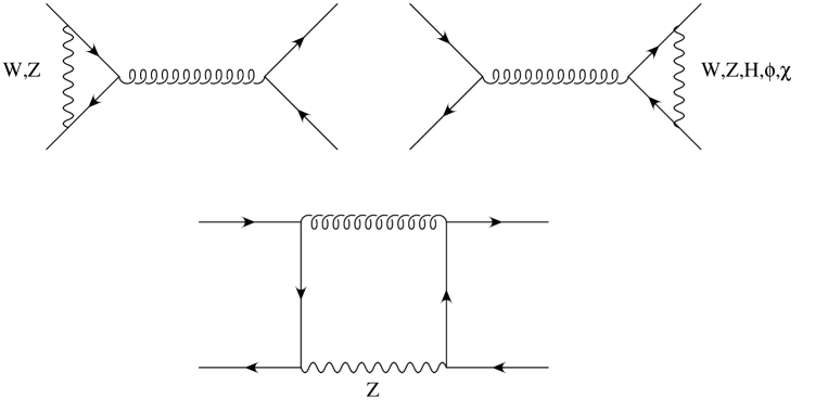
Figure II.1: Sample diagrams for the virtual corrections.

The complete list of Feynman rules can be found for example in Ref. [19]. The second contribution in Eq. (II.1) ${\cal L}_{ct}(\Psi_{R},A_{R},m_{R},g_{R})$ yields the counterterms, which render the calculation ultraviolet (UV)-finite. The diagrams needed here are shown in Fig. II.2. Note that although the electroweak corrections appear here in one-loop approximation, they are the leading-order electroweak contribution.

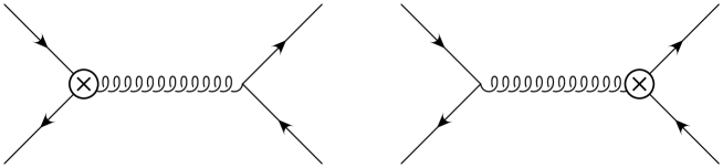
Figure II.2: Counterterm diagrams.

The interference term of the amplitude ${\cal M}(q\bar{q}\to\gamma,Z\to t\bar{t})$ with the corresponding QCD amplitude vanishes as a consequence of the specific colour structure. Terms of order $\alpha_{s}\alpha$ are therefore absent. Thus no renormalization of the coupling constants is required at the order under consideration here. This is different from an electroweak correction to an electroweak amplitude, which would not be UV-finite without coupling-constant renormalization. The whole contribution from the renormalization is given by:

$$\delta|{\cal M}|^{2}=2(\delta Z_{q}+\delta Z_{t})|{\cal M}_{q\bar{q}\to t\bar{t}}|^{2},$$ (II.2)

where $Z_{q}$, $Z_{t}$ denote the wave-function renormalization constants of the incoming light quark and the outgoing top-quark ($Z_{i}=1+\delta Z_{i}$). The squared leading-order QCD amplitude $|{\cal M}_{q\bar{q}\to t\bar{t}}|^{2}$ in $d$ dimensions is given by:

$$|{\cal M}_{q\bar{q}\to t\bar{t}}|^{2}=16\pi^{2}{\alpha_{s}}^{2}(N^{2}-1)(2-\beta^{2}(1-z^{2})-2\varepsilon),$$ (II.3)

where $N$ is the number of colours, ${\alpha_{s}}$ the strong coupling constant and $\beta$ the velocity of the top-quark in the partonic centre-of-mass system:

$$\beta=\sqrt{1-4{{m_{t}}^{2}\over s}}$$ (II.4)

($s$ denotes the partonic centre-of-mass energy squared). The cosine of the scattering angle is denoted by $z$. The parameter of dimensional regularization $\varepsilon$ is defined by

$$d=4-2\varepsilon.$$ (II.5)

For the renormalization of the quark fields we use the on-shell scheme. The renormalization constants in this scheme in terms of self-energy integrals and derivatives thereof can be found for example in Ref. [19]. Before presenting the results, let us add a few technical remarks. We used the Passarino –Veltman reduction scheme [20] to reduce the tensor integrals to scalar one-loop integrals. For the scalar integrals we use the following convention:

$$X_{0}={1\over i\pi^{2}}\int d^{d}\ell{(2\pi\mu)^{2\varepsilon}\over(\ell^{2}-m_{1}^{2}+i\epsilon)\cdots}.$$ (II.6)

For the UV-divergent integrals we define the finite part for the one-point integrals $A_{0}$ and the two-point integrals $B_{0}$ through

$$A_{0}(m^{2}) = m^{2}\Delta+\overline{A}_{0}(m^{2}),$$

$$B_{0}(p^{2},m_{1}^{2},m_{2}^{2}) = \Delta+\overline{B}_{0}(p^{2},m_{1}^{2},m_{2}^{2}),$$ (II.7)

with

$$\Delta=(4\*\pi)^{\varepsilon}\*\Gamma(1+\varepsilon)\*{1\over\varepsilon}={1\over\varepsilon}-\gamma+\ln(4\pi)+O(\varepsilon).$$ (II.8)

The vertex corrections do not contain infrared or mass singularities (IR singularities). They contain only UV singularities, which are removed by the aforementioned renormalization. On the other hand the contribution involving box diagrams are UV-finite but contain IR singularities. In order to regularize the IR singularities, we use dimensional regularization. To simplify their determination, we express the $d$-dimensional four-point scalar integrals $D_{0}^{d}$ in terms of the $(d+2)$-dimensional four-point integrals $D_{0}^{d+2}$ and a combination of three-point integrals in $d$ dimensions. This can be done by the following relation

$$D_{0}^{d+2}=-2\pi D^{d}_{27}$$ (II.9)

where the box integral in 6 dimensions is defined by

$$D^{d=6}(p_{1}^{2},p_{2}^{2},p_{3}^{2},p_{1}\cdot p_{2},p_{2}\cdot p_{3},p_{1}\cdot p_{3},{m_{1}}^{2},{m_{2}}^{2},{m_{3}}^{2},{m_{4}}^{2})[1,\ell_{\mu},\ell_{\mu}\ell_{\nu},\ldots]=$$

$${1\over i\pi^{2}}\int d^{6}\ell\bigg{\{}{[1,\ell_{\mu},\ell_{\mu}\ell_{\nu},\ldots]\over(\ell^{2}-{m_{1}}^{2}+i\varepsilon)((\ell+p_{1})^{2}-{m_{2}}^{2}+i\varepsilon)}$$

$$\times{1\over((\ell+p_{1}+p_{2})^{2}-{m_{3}}^{2}+i\varepsilon)((\ell+p_{1}+p_{2}+p_{3})^{2}-{m_{4}}^{2}+i\varepsilon)}\bigg{\}}$$ (II.10)

and $D^{d}_{27}$ is the coefficient of the metric tensor $g_{\mu\nu}$ appearing in the Passarino –Veltman decomposition [20] of the tensor integral

$$D^{d=6}[\ell_{\mu}\ell_{\nu}]$$ (II.11)

(see Eq. (F.3) in Ref. [20]), which in turn can be expressed as a linear combination of the scalar box integral $D^{d}_{0}$ and scalar triangle integrals $C^{d}_{0}$ in $d$ dimensions. Owing to the finiteness of the box integrals in 6 dimensions the infrared singularities appear only in the three-point integrals.

For the presentation of the results it is convenient to use the leading-order QCD cross section which is given by:

$${d\sigma^{\rm Born}\over dz}={\sigma_{0}}(2-\beta^{2}+\beta^{2}z^{2})$$ (II.12)

with

$${\sigma_{0}}={1\over 8}\pi\alpha_{s}^{2}{N^{2}-1\over N^{2}}{\beta\over s}.$$ (II.13)

A factor $1/(4N^{2})$ from averaging over the incoming spins and colour is included. In a first step we present the corrections to the cross section from the contribution of $Z$ boson and $W$ boson exchange to the light quark–gluon–vertex. The form of this vertex remains unchanged, its normalization is shifted by a factor $(1+\delta F_{D}^{\rm In,W+Z})$, which leads to a shift by

$${d\sigma^{\rm In.,W+Z}\over dz}={d\sigma^{\rm Born}\over dz}2{\rm Re}\delta F_{D}^{\rm In,W+Z}$$ (II.14)

with

$$\delta F_{D}^{\rm In,W+Z}=-{1\over 8}{\alpha\over\pi}\bigg{(}({g_{v}^{q}}^{2}+{g_{a}^{q}}^{2})\*f_{1}(\rho_{z})+2{g_{W}}^{2}\*f_{1}(\rho_{w})\bigg{)}$$ (II.15)

and

$$f_{1}(x)=1+2\*\Big{[}\big{(}1+\ln(x)\big{)}\*\big{(}2\*x+3\big{)}-2\*\big{(}1+x\big{)}^{2}\Big{(}\mbox{Li}_{2}\left(1+{1\over x}\right)-{\pi^{2}\over 6}\Big{)}\Big{]},$$ (II.16)

where we used the definition

$$\rho_{i}={m_{i}^{2}\over s}.$$ (II.17)

In Eq. (II.15), $\alpha={e^{2}\over 4\pi}$ denotes the electromagnetic coupling.
The Cabibbo –Kobayashi–Maskawa mixing matrix has been set to 1. The vector and axial vector couplings of neutral and charged currents are given by

$${g_{v}^{q}} = {1\over 2{s_{W}}{c_{W}}}(T_{3}^{q}-2{s_{W}}^{2}Q_{q}),$$ (II.18)

$${g_{a}^{q}} = {1\over 2{s_{W}}{c_{W}}}T_{3}^{q},$$ (II.19)

$${g_{W}} = {1\over 2\sqrt{2}{s_{W}}},$$ (II.20)

where $Q_{q}$ describes the electric charge in units of the elementary charge $e$, ${s_{W}}$ is the sine of the Weinberg angle (${s_{W}}=\sin({\vartheta_{W}})$ , ${c_{W}}=\cos({\vartheta_{W}})$), and $T_{3}^{q}$ denotes the weak isospin. For the vertex corrections to the final vertex we split the result into the contribution from $Z$ boson exchange, $W$ boson exchange, Higgs exchange and the contributions from the would-be Goldstone bosons including the respective counter terms:

$$d\sigma^{\rm Fin.}=d\sigma^{{\rm Fin.},Z}+d\sigma^{{\rm Fin.},W}+d\sigma^{{\rm Fin.},H}+d\sigma^{{\rm Fin.},\chi}+d\sigma^{{\rm Fin.},\phi}.$$ (II.21)

Note that only the sum has a physically meaningful interpretation. For the individual contributions we obtain

$${d\sigma^{{\rm Fin.},Z}\over dz}={\sigma_{0}}\*{\alpha\over 4\pi}\*\Bigg{\{}-2\*({g_{v}^{t}}^{2}+{g_{a}^{t}}^{2})\*(1+z^{2})$$ (II.22)

$$+ 8\*{1+z^{2}\over(1-\beta^{2})\*s}\*({g_{v}^{t}}^{2}+{g_{a}^{t}}^{2})\*({\overline{A}}_{0}({m_{Z}}^{2})-{\overline{A}}_{0}({m_{t}}^{2}))$$

$$- 4\*\Bigg{[}{1\over(1-\beta^{2})\*\beta^{2}}\*\Big{(}1-\beta^{2}+2\*\beta^{4}\*(1-z^{2})+7\*\beta^{2}\*z^{2}-3\*z^{2}\Big{)}\*\rho_{z}\*({g_{a}^{t}}^{2}+{g_{v}^{t}}^{2})$$

$$+\Big{(}1-5\*z^{2}-3\*\beta^{2}\*(1-z^{2})\Big{)}\*{g_{a}^{t}}^{2}-\Big{(}3+z^{2}-\beta^{2}\*(1-z^{2})\Big{)}\*{g_{v}^{t}}^{2}\Bigg{]}\*{\overline{B}}_{0}^{1}(3,4)$$

$$+ 2\*\Bigg{[}{2\over\beta^{2}}\*f_{2}(z,\beta)\*\rho_{z}\*({g_{a}^{t}}^{2}+{g_{v}^{t}}^{2})-f_{2}(z,\beta)\*({g_{v}^{t}}^{2}-3\*{g_{a}^{t}}^{2})-4\*(1+z^{2})\*{g_{v}^{t}}^{2}\Bigg{]}\*{\overline{B}}_{0}^{3}(1,3)$$

$$+ 2\*s\*\Bigg{[}4\*\Big{(}f_{2}(z,\beta)\*{g_{a}^{t}}^{2}-\Big{(}1+z^{2}\Big{)}\*{g_{v}^{t}}^{2}\Big{)}\*\rho_{z}+{2\over\beta^{2}}\*f_{2}(z,\beta)\*\rho_{z}^{2}\*({g_{v}^{t}}^{2}+{g_{a}^{t}}^{2})$$

$$- (1+\beta^{2})\*(2-\beta^{2}\*(1-z^{2}))\*{g_{v}^{t}}^{2}-\Big{(}2-3\*\beta^{2}+5\*\beta^{2}\*z^{2}+3\*\beta^{4}\*(1-z^{2})\Big{)}\*{g_{a}^{t}}^{2}\Bigg{]}\*C_{0}^{3}$$

$$+ 2\*s\*\Big{[}2\*\rho_{z}\*({g_{v}^{t}}^{2}+{g_{a}^{t}}^{2})+(1-\beta^{2})\*\left({g_{v}^{t}}^{2}-3\*{g_{a}^{t}}^{2}\right)\Big{]}$$

$$\times \*\Big{(}2-\beta^{2}\*(1-z^{2})\Big{)}\*{d\over dp^{2}}\left.B_{0}^{1}(3,4)\right|_{p^{2}={m_{t}}^{2}}\Bigg{\}},$$

with

$$f_{2}(z,\beta)=1-3\*z^{2}-2\*\beta^{2}\*(1-z^{2}).$$ (II.23)

The integrals are defined in the appendix. For the contribution from the $W$ boson we obtain:

$${d\sigma^{{\rm Fin.},W}\over dz}={\sigma_{0}}{\alpha\over 2\pi}\*{g_{W}}^{2}\Bigg{\{}-2\*(1+z^{2})+8\*{1+z^{2}\over(1-\beta^{2})\*s}\*({\overline{A}}_{0}({m_{W}}^{2})-{\overline{A}}_{0}({m_{b}}^{2}))$$ (II.24)

$$- {1\over\beta^{2}}\*\Big{[}{4\over(1-\beta^{2})}\*\Big{(}1-3\*z^{2}-\beta^{2}+7\*\beta^{2}\*z^{2}+2\*\beta^{4}\*(1-z^{2})\Big{)}\*(\rho_{w}-\rho_{b})$$

$$+1-3\*z^{2}-5\*\beta^{2}\*(1+z^{2})-2\*\beta^{4}\*(1-z^{2})\Big{]}\*{\overline{B}}_{0}^{4}(1,2)$$

$$+ {1\over\beta^{2}}\*\Big{[}4\*f_{2}(z,\beta)\*(\rho_{w}-\rho_{b})+1-3\*z^{2}-5\*\beta^{2}\*(1+z^{2})-2\*\beta^{4}\*(1-z^{2})\Big{]}\*{\overline{B}}_{0}^{4}(1,3)$$

$$+ {s\over 4\*\beta^{2}}\*\Big{[}8\*f_{2}(z,\beta)\*(2\*(\rho_{w}-\rho_{b})^{2}-(1+\beta^{2})\*\rho_{b})+1-3\*z^{2}-16\*\beta^{2}-4\*\beta^{2}\*z^{2}+\beta^{4}$$

$$- 11\*\beta^{4}\*z^{2}-2\*\beta^{6}\*(1-z^{2})+8\*\Big{(}1-3\*z^{2}-2\*\beta^{4}\*(1-z^{2})-3\*\beta^{2}\*(1+z^{2})\Big{)}\*\rho_{w}\Big{]}\*C_{0}^{4}$$

$$+ s\*\Big{(}2-\beta^{2}\*(1-z^{2})\Big{)}\*\Big{[}4\*(\rho_{w}-\rho_{b})-(1-\beta^{2})\Big{]}\*{d\over dp^{2}}\left.B_{0}^{4}(1,2)\right|_{p^{2}={m_{t}}^{2}}\Bigg{\}}.$$

The contribution from the Higgs boson is given by

$${d\sigma^{{\rm Fin.},H}\over dz}={\sigma_{0}}{\alpha\over 2\pi}\*{g_{W}}^{2}\*{{m_{t}}^{2}\over{m_{W}}^{2}}\*\Bigg{\{}-(1+z^{2})$$ (II.25)

$$+ 4\*{1+z^{2}\over(1-\beta^{2})\*s}\*({\overline{A}}_{0}({m_{H}}^{2})-{\overline{A}}_{0}({m_{t}}^{2}))$$

$$- 2\*\Big{[}{1\over(1-\beta^{2})\*\beta^{2}}\*\Big{(}1-\beta^{2}+2\*\beta^{4}\*(1-z^{2})+7\*\beta^{2}\*z^{2}-3\*z^{2}\Big{)}\*\rho_{H}$$

$$+ 2\*(1-z^{2})\*(1-\beta^{2})\Big{]}\*{\overline{B}}_{0}^{5}(1,2)$$

$$+ {1\over\beta^{2}}\*\Big{[}2\*f_{2}(z,\beta)\*\rho_{H}+\beta^{2}\*\Big{(}5-3\*z^{2}-4\*\beta^{2}\*(1-z^{2})\Big{)}\Big{]}\*{\overline{B}}_{0}^{3}(1,3)$$

$$+ {2\*s\over\beta^{2}}\*\Big{[}f_{2}(z,\beta)\*\rho_{H}^{2}+3\*\beta^{2}\*(1-z^{2})\*(1-\beta^{2})\*\rho_{H}-\beta^{2}\*(1-\beta^{2})\*\Big{(}2-\beta^{2}\*(1-z^{2})\Big{)}\Big{]}\*C_{0}^{5}$$

$$+ 2\*s\*\Big{(}2-\beta^{2}\*(1-z^{2})\Big{)}\*\Big{[}\rho_{H}-(1-\beta^{2})\Big{]}\*{d\over dp^{2}}\left.B_{0}^{5}(1,2)\right|_{p^{2}={m_{t}}^{2}}\Bigg{\}}.$$

For the unphysical fields $\chi$ and $\phi$ we find

$${d\sigma^{\rm Fin.,\chi}\over dz}={\sigma_{0}}{\alpha\over 2\pi}\*{g_{a}^{t}}^{2}{{m_{t}}^{2}\over{m_{Z}}^{2}}\*\Bigg{\{}-2\*(1+z^{2})-8\*{1+z^{2}\over(1-\beta^{2})\*s}\*({\overline{A}}_{0}({m_{t}}^{2})-{\overline{A}}_{0}({m_{Z}}^{2}))$$ (II.26)

$$+ {2\over\beta^{2}}\*\Big{[}2\*f_{2}(z,\beta)\*\rho_{z}+\beta^{2}\*(1+z^{2})\Big{]}\*{\overline{B}}_{0}^{3}(1,3)$$

$$- {4\over\beta^{2}\*(1-\beta^{2})}\*\Big{[}1-\beta^{2}+2\*\beta^{4}\*(1-z^{2})+7\*\beta^{2}\*z^{2}-3\*z^{2}\Big{]}\*\rho_{z}\*{\overline{B}}_{0}^{1}(3,4)$$

$$+ {4\*s\over\beta^{2}}\*\Big{[}f_{2}(z,\beta)\*\rho_{z}^{2}+\beta^{2}\*(1-z^{2})\*(1-\beta^{2})\*\rho_{z}\Big{]}\*C_{0}^{3}$$

$$+ 4\*s\*\Big{(}2-\beta^{2}\*(1-z^{2})\Big{)}\*\rho_{z}\*{d\over dp^{2}}\left.B_{0}^{1}(3,4)\right|_{p^{2}={m_{t}}^{2}}\Bigg{\}},$$

$$d\sigma^{\rm Fin.,\phi}={\sigma_{0}}\*{\alpha\over 2\pi}\*{g_{W}}^{2}\Bigg{\{}-{1\over 4\*\rho_{w}}\*y_{s}\*(1+z^{2})+{(1+z^{2})\over(1-\beta^{2})\*{m_{W}}^{2}}\*y_{s}\*({\overline{A}}_{0}({m_{W}}^{2})-{\overline{A}}_{0}({m_{b}}^{2}))$$ (II.27)

$$- {1\over 8\*\beta^{2}\*(1-\beta^{2})}\*\Big{[}4\*\Big{(}1-3\*z^{2}-\beta^{2}+7\*\beta^{2}\*z^{2}+2\*\beta^{4}\*(1-z^{2})\Big{)}\*y_{s}$$

$$- 16\*\Big{(}1-3\*z^{2}-\beta^{2}+7\*\beta^{2}\*z^{2}+2\*\beta^{4}\*(1-z^{2})\Big{)}\*\rho_{b}\*y_{\phi}-16\*\beta^{2}\*(1-\beta^{2})^{2}\*(1-z^{2})\*y_{\phi}$$

$$+ (1-\beta^{2})^{2}\*\Big{(}1-3\*z^{2}+3\*\beta^{2}\*(1+z^{2})-2\*\beta^{4}\*(1-z^{2})\Big{)}\*\rho_{w}^{-1}\Big{]}\*{\overline{B}}_{0}^{4}(1,2)$$

$$+ {1\over 8\*\beta^{2}}\*\Big{[}4\*f_{2}(z,\beta)\*(y_{s}-4y_{\phi}\*\rho_{b}-2\*\beta^{2}\*y_{\phi})$$

$$+ (1-\beta^{2})\*\Big{(}1-3\*z^{2}+3\*\beta^{2}\*(1+z^{2})-2\*\beta^{4}\*(1-z^{2})\Big{)}\*\rho_{w}^{-1}\Big{]}\*{\overline{B}}_{0}^{4}(1,3)$$

$$+ {s\over 32\*\beta^{2}}\*\bigg{[}16\*f_{2}(z,\beta)\*(y_{s}\*\rho_{w}+4\*\rho_{b}^{2}\*y_{\phi}-8\*\rho_{b}^{2})+8\*(1-\beta^{2})^{2}\*\Big{(}1-3\*z^{2}+2\*\beta^{2}\*(1-z^{2})\Big{)}$$

$$- 16\*\Big{(}1-3\*z^{2}+\beta^{2}+9\*\beta^{2}\*z^{2}+2\*\beta^{4}\*(1-z^{2})\Big{)}\*\rho_{b}\*y_{\phi}$$

$$- 4\*(1-\beta^{2})\*\Big{(}1-3\*z^{2}-11\*\beta^{2}-3\*\beta^{2}\*z^{2}+2\*\beta^{4}\*(1-z^{2})\Big{)}\*y_{\phi}$$

$$+ (1-\beta^{2})^{2}\*\Big{(}1-3\*z^{2}-7\*\beta^{2}+\beta^{2}\*z^{2}+2\*\beta^{4}\*(1-z^{2})\Big{)}\*\rho_{w}^{-1}\bigg{]}\*C_{0}^{4}$$

$$+ {s\over 8}\*\Big{[}4\*y_{s}-16\*\rho_{b}\*y_{\phi}+8\*(1-\beta^{2})\*y_{\phi}-{(1-\beta^{2})^{2}\over\rho_{w}}\Big{]}$$

$$\times\Big{(}2-\beta^{2}\*(1-z^{2})\Big{)}\*{d\over dp^{2}}\left.B_{0}^{4}(1,2)\right|_{p^{2}={m_{t}}^{2}}\Bigg{\}},$$

where we used the abbreviations:

$$y_{s}=1-\beta^{2}+4\rho_{b},$$ (II.28)

$$y_{\phi}={{m_{b}}^{2}\over{m_{W}}^{2}}.$$ (II.29)

Again only terms proportional to ${g_{v}^{t}}^{2},{g_{a}^{t}}^{2}$ or ${g_{W}}^{2}$ are present. Let us now discuss the contribution from the box diagrams. To the order $\alpha{\alpha_{s}}^{2}$ considered here, we can distinguish two different contributions:

1. The (box-type) electroweak correction to the QCD Born amplitude, interfering with the QCD Born amplitude.

2. The QCD box diagram interfering with the electroweak Born amplitude.

In the following we will call the first the electroweak-box (EW-box), and the second the QCD-box contribution. For the EW-box we obtain

$${d\sigma^{\rm EW-box}\over dz}={\sigma_{0}}\*{\alpha\over\pi}\*\Bigg{\{}-{2\*(1-\beta^{2})\over\beta\*(1-\beta^{2}\*z^{2})}\*\Bigg{[}z\*\bigg{(}1+2\*\beta^{2}-\beta^{2}\*z^{2}\bigg{)}\*{g_{v}^{q}}\*{g_{v}^{t}}+2\*\beta\*{g_{a}^{q}}\*{g_{a}^{t}}\Bigg{]}\*{\overline{B}}_{0}^{1}(1,4)$$ (II.30)

$$+ {2\*(1-2\*\beta^{2}+\beta^{2}\*z^{2})\over 1-\beta\*z}\*\Bigg{[}{g_{v}^{q}}\*{g_{v}^{t}}+{g_{a}^{q}}\*{g_{a}^{t}}\bigg{]}\*{\overline{B}}_{0}^{1}(2,4)+{4\over\beta}\*\Bigg{[}{g_{v}^{q}}\*{g_{v}^{t}}\*z+{g_{a}^{q}}\*{g_{a}^{t}}\*\beta\Bigg{]}\*{\overline{B}}_{0}^{1}(1,3)$$

$$- {2\*(1-\beta^{2})\over\beta\*(1-\beta^{2}\*z^{2})}\*\Bigg{[}z\*\bigg{(}1+2\*\beta^{2}-\beta^{2}\*z^{2}\bigg{)}\*{g_{v}^{q}}\*{g_{v}^{t}}+2\*{g_{a}^{q}}\*{g_{a}^{t}}\*\beta\Bigg{]}\*{\overline{B}}_{0}^{1}(3,4)$$

$$- {2\over 1+\beta\*z}\*(1-2\*\beta^{2}+\beta^{2}\*z^{2})\*\Bigg{[}{g_{v}^{q}}\*{g_{v}^{t}}-{g_{a}^{q}}\*{g_{a}^{t}}\Bigg{]}\*{\overline{B}}_{0}^{2}(2,4)$$

$$+ s\*{2\*(1-\beta^{2})\over\beta\*(1-\beta^{2}\*z^{2})\*(1-\rho_{z})}\*\Bigg{[}z\*\bigg{(}1+\beta^{4}\*z^{2}-\beta^{2}\*z^{2}-\beta^{4}+2\*\beta^{2}$$

$$+ (\beta^{4}\*z^{2}+2\*\beta^{2}\*z^{2}-2-\beta^{4})\*\rho_{z}-(-2\*\beta^{2}-1+\beta^{2}\*z^{2})\*\rho_{z}^{2}\bigg{)}\*{g_{v}^{q}}\*{g_{v}^{t}}$$

$$+ 2\*\beta\*\bigg{(}\beta^{2}\*z^{2}-(1-\beta^{2}\*z^{2})\*\rho_{z}+\rho_{z}^{2}\bigg{)}\*{g_{a}^{q}}\*{g_{a}^{t}}\Bigg{]}\*C_{0}(1,3,4)$$

$$+ s\*{1\over(1-\beta\*z)\*(1-\rho_{z})^{2}}\*\Bigg{[}\bigg{(}2\*(\beta^{2}\*z^{2}-2\*\beta^{2}+1)\*\rho_{z}^{3}$$

$$- (4-5\*\beta^{2}+2\*\beta^{3}\*z+\beta^{2}\*z^{2}-2\*\beta^{3}\*z^{3}-\beta^{4}+\beta^{4}\*z^{2})\*\rho_{z}^{2}$$

$$+ \beta\*(\beta^{3}\*z^{4}+4\*z-2\*\beta^{3}\*z^{2}-4\*\beta+\beta^{3})\*\rho_{z}+3\*\beta^{2}\*z^{2}-2\*\beta^{3}\*z^{3}$$

$$+ 2-4\*\beta\*z-\beta^{2}-\beta^{4}\*z^{2}+\beta^{4}\*z^{4}+2\*\beta^{3}\*z\bigg{)}\*{g_{v}^{q}}\*{g_{v}^{t}}$$

$$+ 2\*\bigg{(}(\beta^{2}\*z^{2}-2\*\beta^{2}+1)\*\rho_{z}^{3}+(-3+4\*\beta^{2}-2\*\beta^{3}\*z+\beta^{3}\*z^{3}-\beta^{2}\*z^{2}+\beta\*z)\*\rho_{z}^{2}$$

$$+ (3-3\*\beta\*z+\beta^{3}\*z-3\*\beta^{2}+2\*\beta^{2}\*z^{2})\*\rho_{z}-2\*\beta^{2}\*z^{2}+\beta^{2}-\beta^{3}\*z+\beta^{3}\*z^{3}$$

$$+ 2\*\beta\*z-1\bigg{)}\*{g_{a}^{q}}\*{g_{a}^{t}}\bigg{]}\*C_{0}^{1}(2,3,4)$$

$$- s\*{1\over(1+\beta\*z)\*(1-\rho_{z})^{2}}\*\Bigg{[}\bigg{(}3\*\beta^{2}\*z^{2}+2\*\beta^{3}\*z^{3}+2+4\*\beta\*z-\beta^{2}-\beta^{4}\*z^{2}$$

$$+ \beta^{4}\*z^{4}-2\*\beta^{3}\*z+\beta\*(\beta^{3}\*z^{4}-4\*z-2\*\beta^{3}\*z^{2}-4\*\beta+\beta^{3})\*\rho_{z}$$

$$- (4-5\*\beta^{2}-2\*\beta^{3}\*z+\beta^{2}\*z^{2}+2\*\beta^{3}\*z^{3}-\beta^{4}+\beta^{4}\*z^{2})\*\rho_{z}^{2}$$

$$+ 2\*(\beta^{2}\*z^{2}-2\*\beta^{2}+1)\*\rho_{z}^{3}\bigg{)}\*{g_{v}^{q}}\*{g_{v}^{t}}+2\*\bigg{(}+2\*\beta^{2}\*z^{2}-\beta^{2}-\beta^{3}\*z+\beta^{3}\*z^{3}+2\*\beta\*z+1$$

$$+ (-3-3\*\beta\*z+\beta^{3}\*z+3\*\beta^{2}-2\*\beta^{2}\*z^{2})\*\rho_{z}$$

$$+ (3-4\*\beta^{2}-2\*\beta^{3}\*z+\beta^{3}\*z^{3}+\beta^{2}\*z^{2}+\beta\*z)\*\rho_{z}^{2}$$

$$- (\beta^{2}\*z^{2}-2\*\beta^{2}+1)\*\rho_{z}^{3}\bigg{)}\*{g_{a}^{q}}\*{g_{a}^{t}}\Bigg{]}\*C_{0}^{2}(2,3,4)$$

$$+ {2\*\beta^{2}\*(1-z^{2})\over(1-\beta\*z)\*(1-\rho_{z})^{2}}\*\Bigg{[}\bigg{(}3-\beta^{2}-2\*\beta\*z\*(1-\beta\*z)-(1-2\*\beta\*z+\beta^{2})\*\rho_{z}+2\*\rho_{z}^{2}\bigg{)}\*{g_{v}^{q}}\*{g_{v}^{t}}$$

$$+ 2\*\big{(}\beta\*z-(1-\beta\*z)\*\rho_{z}+\rho_{z}^{2}\big{)}\*{g_{a}^{q}}\*{g_{a}^{t}}\Bigg{]}\*s\*{D^{d=6,EW1}_{0}}$$

$$- {2\*\beta^{2}\*(1-z^{2})\over(1+\beta\*z)\*(1-\rho_{z})^{2}}\*\Bigg{[}\bigg{(}3-\beta^{2}+2\*\beta\*z\*(1+\beta\*z)-(1+\beta^{2}+2\*\beta\*z)\*\rho_{z}+2\*\rho_{z}^{2}\bigg{)}\*{g_{v}^{q}}\*{g_{v}^{t}}$$

$$+ 2\*\bigg{(}\beta\*z+(1+\beta\*z)\*\rho_{z}-\rho_{z}^{2}\bigg{)}\*{g_{a}^{q}}\*{g_{a}^{t}}\Bigg{]}\*s\*{D^{d=6,EW2}_{0}}\Bigg{\}}$$

$$- {1\over 64\*\pi}\*{\alpha_{s}}\*{1\over N^{2}}\*\beta\*B\*\bigg{[}(1-\beta\*z)\*C_{0}^{1}(1,2,4)-(1+\beta\*z)\*C_{0}^{2}(1,2,4)\bigg{]}+{\cal O}(\varepsilon),$$

with

$$B=-8\*\pi\*\alpha\*{\alpha_{s}}\*(N^{2}-1)\*{s\over s-{m_{Z}}^{2}}\*\bigg{(}(d-2-\beta^{2}\*(1-z^{2}))\*{g_{v}^{q}}\*{g_{v}^{t}}+\beta\*z\*(d-2)\*(d-3)\*{g_{a}^{q}}\*{g_{a}^{t}}\bigg{)}.$$ (II.31)

Note that the contribution $d\sigma^{\rm EW-box}$ is UV-finite, as already mentioned. This can be easily checked by replacing the ${\overline{B}}_{0}$ integrals by $\Delta$ and verifying that this contribution indeed vanishes. Since we are using box integrals in $d=6$ dimensions, the IR singularities appear only in the three-point integrals. In particular, in the above result, only the last line in Eq. (II.30) is singular. As a consequence only this term needs to be evaluated in $d$ dimensions. Note that owing to the structure of the IR-singularities in QCD we will not pick up finite terms of the form $\varepsilon/\varepsilon$. They will cancel with the corresponding terms in the real corrections, as we will show in the next section, where the real corrections are discussed.

For the QCD-box we find

$${d\sigma^{\rm QCD}\over dz} = {\sigma_{0}}{\alpha\over\pi}\*{1\over(1-\rho_{z})}\Bigg{\{}+{2\over\beta}\*\Bigg{[}\beta\*{g_{a}^{q}}\*{g_{a}^{t}}+z\*{g_{v}^{q}}\*{g_{v}^{t}}\Bigg{]}\*{\overline{B}}_{0}^{6}(1,3)$$ (II.32)

$$+ 2\*{1-\beta^{2}\over\beta\*(1-\beta^{2}\*z^{2})}\*\Bigg{[}z\*\bigg{(}-1-2\*\beta^{2}+\beta^{2}\*z^{2}\bigg{)}\*{g_{v}^{q}}\*{g_{v}^{t}}-\beta\*\bigg{(}1+\beta^{2}\*z^{2}\bigg{)}\*{g_{a}^{q}}\*{g_{a}^{t}}\Bigg{]}\*{\overline{B}}_{0}^{1}(1,4)$$

$$+ {1\over 1-\beta\*z}\*\Bigg{[}\bigg{(}1-2\*\beta^{2}+\beta^{2}\*z^{2}\bigg{)}\*{g_{v}^{q}}\*{g_{v}^{t}}-\beta\*(\beta-z)\*(1+\beta\*z)\*{g_{a}^{q}}\*{g_{a}^{t}}\Bigg{]}\*{\overline{B}}_{0}^{1}(2,4)$$

$$- {1\over 1+\beta\*z}\*\Bigg{[}\bigg{(}1-2\*\beta^{2}+\beta^{2}\*z^{2}\bigg{)}\*{g_{v}^{q}}\*{g_{v}^{t}}+\beta\*(\beta+z)\*(1-\beta\*z)\*{g_{a}^{q}}\*{g_{a}^{t}}\Bigg{]}\*{\overline{B}}_{0}^{2}(2,4)$$

$$+ {1-\beta^{2}\over\beta\*(1-\beta^{2}\*z^{2})}\*\Bigg{[}z\*\bigg{(}1+\beta^{2}+\beta^{2}\*(1-\beta^{2})\*(1-z^{2})\bigg{)}\*{g_{v}^{q}}\*{g_{v}^{t}}$$

$$+ \beta\*\bigg{(}1+\beta^{2}\*z^{2}\bigg{)}\*{g_{a}^{q}}\*{g_{a}^{t}}\Bigg{]}\*s\*{C_{0}^{\rm QCD1}(1,3,4)}$$

$$- {\beta^{2}\*(1-z^{2})\over 1+\beta\*z}\*\Bigg{[}\bigg{(}3+2\*\beta\*z\*(1+\beta\*z)-\beta^{2}\bigg{)}\*{g_{v}^{q}}\*{g_{v}^{t}}+2\*\beta\*z\*{g_{a}^{q}}\*{g_{a}^{t}}\Bigg{]}\*s\*{D^{d=6,2}_{0}}$$

$$+ {\beta^{2}\*(1-z^{2})\over 1-\beta\*z}\*\Bigg{[}\bigg{(}3-2\*\beta\*z\*(1-\beta\*z)-\beta^{2}\bigg{)}\*{g_{v}^{q}}\*{g_{v}^{t}}+2\*\beta\*z\*{g_{a}^{q}}\*{g_{a}^{t}}\Bigg{]}\*s\*{D^{d=6,1}_{0}}\Bigg{\}}$$

$$- {1\over 64\*\pi}\*{\alpha_{s}}\*{1\over N^{2}}\*\beta\*B\*\bigg{[}(1-\beta\*z)\*C_{0}^{1}(1,2,4)-(1+\beta\*z)\*C_{0}^{2}(1,2,4)\bigg{]}+{\cal O}(\varepsilon).$$

Combining the two results in Eqs. (II.30) and (II.32), the IR-divergent part is thus given by

$$- {{\alpha_{s}}\over 32\*\pi}\*{1\over N^{2}}\*\beta\*B\*\bigg{[}(1-\beta\*z)\*C_{0}^{1}(1,2,4)-(1+\beta\*z)\*C_{0}^{2}(1,2,4)\bigg{]}$$ (II.33)

$$= -{{\alpha_{s}}\over 16\*\pi}\*{1\over N^{2}}\*{\beta\over s}\*B\*\bigg{[}{s_{qt}}\*C_{0}^{1}(1,2,4)-{s_{q{\bar{t}}}}\*C_{0}^{2}(1,2,4)\bigg{]}$$

In particular, we obtain

$$-{{\alpha_{s}}\over 16\*\pi}\*{1\over N^{2}}\*{\beta\over s}\*B\*\bigg{[}{s_{qt}}\*C_{0}^{1}(1,2,4)-{s_{q{\bar{t}}}}\*C_{0}^{2}(1,2,4)\bigg{]}$$ (II.34)

$$= {{\alpha_{s}}\over 32\*\pi}\*{1\over N^{2}}\*{\beta\over s}\*\*B\*(4\pi)^{\varepsilon}\Gamma(1+\varepsilon)\bigg{[}{2\over\varepsilon}\ln\left({{s_{q{\bar{t}}}}\over{s_{qt}}}\right)+g({s_{qt}})-g({s_{q{\bar{t}}}})\bigg{]},$$

with $s_{ij}=2k_{i}\cdot k_{j}$, where we have used

$$C_{0}^{1}(1,2,4)={1\over i\pi^{2}}\int d^{d}\ell{1\over\ell^{2}(\ell+k_{q})^{2}((\ell+k_{t})^{2}-{m_{t}}^{2})}$$

$$=-{1\over 2}(4\pi)^{\varepsilon}\Gamma(1+\varepsilon){1\over{s_{qt}}}\bigg{(}{1\over\varepsilon^{2}}+{1\over\varepsilon}\ln\left({{m_{t}}^{2}\mu^{2}\over{s_{qt}}^{2}}\right)+g({s_{qt}})\bigg{)}+{\cal O}(\varepsilon),$$ (II.35)

with

$$g({s_{qt}})=-\ln\left({{s_{qt}}\over\mu^{2}}\right)\*\ln\left({{m_{t}}^{2}\over{s_{qt}}}\right)+{1\over 2}\*\ln\left({{s_{qt}}\over\mu^{2}}\right)^{2}-2\*\mbox{Li}_{2}\left({{s_{qt}}-{m_{t}}^{2}\over{s_{qt}}}\right)-{1\over 2}\*\ln\left({{m_{t}}^{2}\over{s_{qt}}}\right)^{2}.$$ (II.36)

We note that the divergent three-point integral

$${1\over i\pi^{2}}\int{1\over\ell^{2}(\ell+k_{q})^{2}((\ell+k_{q}+k_{{\bar{q}}})^{2}-{m_{Z}}^{2})},$$ (II.37)

which could in principle also appear, cancels in the calculation.

III Real corrections

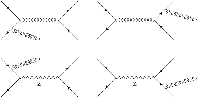
Figure III.1: Sample diagrams for the real corrections.

As mentioned in the previous section the contribution from the box diagrams is IR-divergent. To render the corrections to the total cross section finite we need to include the real corrections at the same order. A few sample diagrams are shown in Fig. III.1. The diagram containing the triple gluon vertex (see Fig. III.2) does not contribute because of the colour structure. The calculation of the real corrections is straightforward. The phase-space integration over the regions where the emitted gluon is soft will produce the IR singular contribution needed to cancel the corresponding singularities in the virtual corrections. Note that owing to the colour structure no collinear singularities appear, because the interference between the two diagrams, where the gluon is emitted from the initial state, vanishes. As a consequence no factorization of initial-state singularities is required. To extract the IR divergences, we use the so-called subtraction method [21, 22, 23]. The basic idea of the subtraction method is to add and subtract a term in such a way that the singularities appearing in the real corrections are matched point-wise and that the term is simple enough to be integrated analytically in $d$ dimensions over the full phase space. Given that the same term is added and subtracted, this procedure does not change the result. The analytically integrated term is combined with the virtual corrections, while the unintegrated term is combined with the real corrections.

Figure III.2: Amplitude containing the triple gluon vertex. The diagram does not contribute here because of the colour structure.

Given that the term combined with the real corrections match point-wise the singularities of the squared matrix element, the integration can be done numerically in 4 dimensions. Because of the universal structure of soft and mass singularities in QCD, the subtraction terms can be constructed in a very general way. For further details on the subtraction method, we refer to Refs. [21, 23]. Here we just reproduce the necessary equations required for the case at hand.

Using the subtraction method the NLO contribution to the cross section can be symbolically written as [21, 23]

$$\sigma_{\rm NLO}(k_{q},k_{{\bar{q}}})=\sigma_{\rm V}(k_{q},k_{{\bar{q}}})+\sigma_{\rm R}(k_{q},k_{{\bar{q}}})=$$ (III.1)

$$\int_{3}\Bigg{\{}\left[d\sigma_{\rm R}(k_{q},k_{{\bar{q}}},k_{t},k_{{\bar{t}}},k_{g})\right]_{\varepsilon=0}-\left[\sum_{\rm dipoles}\left(d\sigma_{\rm LO}\otimes dV_{\rm dipole}\right)(k_{q},k_{{\bar{q}}},k_{t},k_{{\bar{t}}},k_{g})\right]_{\varepsilon=0}\Bigg{\}}$$

$$+ \int_{2}\left[d\sigma_{\rm V}(k_{q},k_{{\bar{q}}},k_{t},k_{{\bar{t}}})+d\sigma_{\rm LO}(k_{q},k_{{\bar{q}}},k_{t},k_{{\bar{t}}})\otimes({\bf I}_{q}+{\bf I}_{\bar{q}})\right]_{\varepsilon=0}$$

$$+ \int dx\int_{2}d\sigma_{\rm LO}(xk_{q},k_{{\bar{q}}},k_{t},k_{{\bar{t}}})\otimes({\bf K}_{q}+{\bf P}_{q})$$

$$+ \int dx\int_{2}d\sigma_{\rm LO}(k_{q},xk_{{\bar{q}}},k_{t},k_{{\bar{t}}})\otimes({\bf K}_{\bar{q}}+{\bf P}_{\bar{q}}).$$

Here $d\sigma_{\rm R}$, $d\sigma_{\rm V}$ denote the real and virtual corrections to the cross section. In particular we have

$$d\sigma_{\rm V}=d\sigma^{\rm In.}+d\sigma^{\rm Fin.}+d\sigma^{\rm EW-box}+d\sigma^{\rm QCD-box}.$$ (III.2)

In Eq. (III.1) we label the integral symbols with an index 2 or 3 to indicate that the phase-space integral runs over a 2- or 3-particle final state. The terms of the form

$$d\sigma_{\rm LO}\otimes{\bf F}$$ (III.3)

with ${\bf F}={\bf P},{\bf K},dV_{\rm dipole}$ deserve some explanation. In general the symbol ‘$\otimes$’ introduces spin as well as colour correlation between the operator $F$ and the leading-order amplitude, which is a vector in colour space. Note that for the case studied here, where the gluon is always emitted from a quark line, no spin correlation appears. For the contribution from the integrated dipoles we obtain

$$d\sigma_{\rm LO}(k_{q},k_{{\bar{q}}},k_{t},k_{{\bar{t}}})\otimes{\cal I}={1\over 32\pi}{1\over 4N^{2}}{\beta\over s}\left\langle q{\bar{q}}\to t{\bar{t}}\left|{\bf I}_{q}+{\bf I}_{\bar{q}}\right|q{\bar{q}}\to t{\bar{t}}\,\right\rangle_{\alpha{\alpha_{s}}}$$ (III.4)

$$= -{{\alpha_{s}}\over 32\pi^{2}}{1\over 4N^{2}}{\beta\over s}{(4\pi)^{\varepsilon}\over\Gamma(1-\varepsilon)}\bigg{\{}{2\over\varepsilon}\ln\left({{s_{q{\bar{t}}}}\over{s_{qt}}}\right)+H({s_{qt}})-H({s_{q{\bar{t}}}})\bigg{\}}$$

$$\times \left\langle q{\bar{q}}\to t{\bar{t}}\left|T_{q}T_{t}\right|q{\bar{q}}\to t{\bar{t}}\,\right\rangle,$$

with

$$H({s_{qt}}) = -{1\over 2}\*\ln\left({{m_{t}}^{2}\over{s_{qt}}}\right)^{2}-\ln\left({{m_{t}}^{2}\over{s_{qt}}}\right)\*\ln\left({{s_{qt}}\over Q^{2}({s_{qt}},{m_{t}})}\right)$$ (III.5)

$$- \ln\left({{m_{t}}^{2}\over Q^{2}({s_{qt}},{m_{t}})}\right)\*\ln\left({{s_{qt}}\over Q^{2}({s_{qt}},{m_{t}})}\right)$$

$$+ \ln\left({\mu^{2}\over{s_{qt}}}\right)\*\ln\left({{m_{t}}^{2}\over{s_{qt}}}\right)+{1\over 2}\*\ln\left({\mu^{2}\over{s_{qt}}}\right)^{2}+{6\over 2}\*\ln\left({\mu^{2}\over{s_{qt}}}\right)$$

$$+ \ln\left({{s_{qt}}\over Q^{2}({s_{qt}},{m_{t}})}\right)-2\mbox{Li}_{2}\left({{s_{qt}}\over Q^{2}({s_{qt}},{m_{t}})}\right)-{{m_{t}}^{2}\over{s_{qt}}}\*\ln\left({{m_{t}}^{2}\over Q^{2}({s_{qt}},{m_{t}})}\right)$$

$$- 3\ln\left({Q({s_{qt}},{m_{t}})-{m_{t}}\over Q({s_{qt}},{m_{t}})}\right)-{3{m_{t}}\over Q({s_{qt}},{m_{t}})+{m_{t}}}+{\pi^{2}\over 6}.$$

Following Ref. [21] we used the bra-ket notation to represent the leading-order amplitude as vector in colour space:

$$\left|q{\bar{q}}\to t{\bar{t}}\,\right\rangle.$$

In the derivation we used the following result for ${\bf I}$

$${\bf I}_{q}(\varepsilon,\mu^{2};\{\},p_{a})=-{{\alpha_{s}}\over 2\pi}{(4\pi)^{\varepsilon}\over\Gamma(1-\varepsilon)}\Bigg{\{}{1\over{C_{F}}}T_{t}T_{q}\Bigg{[}{C_{F}}\left({{\mu^{2}}\over{s_{qt}}}\right)^{\varepsilon}\left({\cal V}_{Q}({s_{qt}},{m_{t}},0;\varepsilon,\kappa)-{\pi^{2}\over 3}\right)$$ (III.6)

$$+ \Gamma_{Q}(\mu,{m_{t}};\varepsilon)+\gamma_{q}\*\ln\left({{\mu^{2}}\over{s_{qt}}}\right)+\gamma_{q}+K_{q}\Bigg{]}$$

$$+ {1\over{C_{F}}}T_{t}T_{q}\Bigg{[}{C_{F}}\left({{\mu^{2}}\over{s_{qt}}}\right)^{\varepsilon}\left({\cal V}_{q}({s_{qt}},0,{m_{t}};\varepsilon,2/3)-{\pi^{2}\over 3}\right)+{\gamma_{q}\over\varepsilon}+\gamma_{q}\*\ln\left({{\mu^{2}}\over{s_{qt}}}\right)+\gamma_{q}+K_{q}\Bigg{]}$$

$$+ (t\leftrightarrow{\bar{t}})\Bigg{\}},$$

which can be easily obtained from Ref. [23]. The definitions of ${\cal V}_{Q},{\cal V}_{q},\Gamma_{Q},\gamma_{q},K_{q}$ can be found in Ref. [23]. The result for ${\bf I}_{\bar{q}}$ can be obtained from the above result by the replacement $(q\leftrightarrow{\bar{q}})$. The $T_{t},T_{q}$ appearing in the above equation are colour-charge operators, which act on the leading-order amplitudes that are vectors in colour space. The calculation of this specific contribution was further simplified by noting that, because of the simple colour structure of the process at hand, the following relation holds:

$$\left\langle q{\bar{q}}\to t{\bar{t}}\left|T_{q}T_{t}\right|q{\bar{q}}\to t{\bar{t}}\,\right\rangle=-\left\langle q{\bar{q}}\to t{\bar{t}}\left|T_{q}T_{\bar{t}}\right|q{\bar{q}}\to t{\bar{t}}\,\right\rangle$$

$$=-\left\langle q{\bar{q}}\to t{\bar{t}}\left|T_{\bar{q}}T_{t}\right|q{\bar{q}}\to t{\bar{t}}\,\right\rangle=\left\langle q{\bar{q}}\to t{\bar{t}}\left|T_{\bar{q}}T_{\bar{t}}\right|q{\bar{q}}\to t{\bar{t}}\,\right\rangle.$$ (III.7)

The square of the colour-correlated tree amplitudes is given by

$$\left\langle q{\bar{q}}\to t{\bar{t}}\left|T_{q}T_{t}\right|q{\bar{q}}\to t{\bar{t}}\,\right\rangle$$ (III.8)

$$= -32\pi^{2}\alpha{\alpha_{s}}(N^{2}-1)\*{s\over s-{m_{Z}}^{2}}\bigg{(}(d-2-\beta^{2}(1-z^{2}))\*{g_{v}^{q}}\*{g_{v}^{t}}+\beta\*z\*(d-2)\*(d-3)\*{g_{a}^{q}}\*{g_{a}^{t}}\bigg{)}$$

$$= 4\pi B,$$

with $B$ as defined in Eq. (II.31). Comparing Eq. (II.34) with Eqs. (III.4), (III.8), it is easy to see that when combining the real and virtual corrections the IR singularities indeed cancel. In addition, as promised already in the previous section, we see that indeed no $\varepsilon/\varepsilon$ terms appear, which must be due to the ‘$d$-dimensional’ factorization of the infrared singularities. The ${\bf K}$ and ${\bf P}$ operators can be calculated along the same lines as described above for the ${\bf I}$ operator. In particular we obtain

$${\bf K}_{q}=-{{\alpha_{s}}\over 2\pi}T_{t}T_{q}\bigg{\{}K(x,{s_{qt}},{m_{t}})-K(x,{s_{q{\bar{t}}}},{m_{t}})\bigg{\}},$$ (III.9)

with

$$K(x,{s_{qt}},{m_{t}})=\bigg{[}J_{gQ}\left(x,{{m_{t}}^{2}\over{s_{qt}}}\right)\bigg{]}_{+}+2\bigg{[}{1\over 1-x}\bigg{]}_{+}\ln\left({(2-x){s_{qt}}\over(2-x){s_{qt}}+{m_{t}}^{2}}\right)$$

$$+ \delta(1-x)\Bigg{[}{{m_{t}}^{2}\over{s_{qt}}}\ln\left({m_{t}}^{2}\over{s_{qt}}+{m_{t}}^{2}\right)+{1\over 2}\*{{m_{t}}^{2}\over{s_{qt}}+{m_{t}}^{2}}+{3\over 2}{2{m_{t}}\over\sqrt{{s_{qt}}+{m_{t}}^{2}}+{m_{t}}}$$

$$+ {3\over 2}\ln\left({{s_{qt}}-2{m_{t}}\sqrt{{s_{qt}}+{m_{t}}^{2}}+2{m_{t}}^{2}\over{s_{qt}}}\right)\Bigg{]}+P^{qq}_{\rm reg}(x)\ln\left({(1-x){s_{qt}}\over(1-x){s_{qt}}+{m_{t}}^{2}}\right),$$

where the regular part $P^{qq}_{\rm reg}$ of the evolution kernel $P^{qq}(x)$ is given by

$$P^{qq}_{\rm reg}(x)=-(1+x),$$ (III.11)

and the Plus prescription defines distributions in the usual way, through

$$\left[{F(z)}\right]_{+}=\lim_{\eta\rightarrow 0}\left\{\Theta(1-z-\eta)F(z)-\delta(1-z-\eta)\int_{0}^{1-\eta}F(y)dy\right\}.$$ (III.12)

The function $\left[{J_{gQ}}\right]_{+}$ is given in Eq. (5.58) of Ref. [23], and we reproduce it here explicitly:

$$\left[{J_{gQ}(x,y^{2})}\right]_{+} = \left[{{1-x\over 2(1-x+y^{2})^{2}}-{2\over 1-x}\left(1+\ln(1-x+y^{2})\right)}\right]_{+}$$ (III.13)

$$+ \left[{{2\over 2-x}}\right]_{+}\ln(2+y^{2}-x).$$

For the ${\bf P}$ operator we find

$${\bf P}_{q}={{\alpha_{s}}\over 2\pi}P^{qq}(x)T_{t}T_{q}\ln\left({{s_{q{\bar{t}}}}\over{s_{qt}}}\right),$$ (III.14)

with

$$P^{qq}(x)=P^{qq}_{\rm reg}(x)+\left[{2\over 1-x}\right]_{+}+{3\over 2}\delta(1-x).$$ (III.15)

Note that in deriving the above relations we used again relation Eq. (III.7) to simplify the colour charge algebra. The corresponding results for the antiquark give the same contribution for the ${\bf K}$ and ${\bf P}$ operators. Note that when calculating

$$\int dx\int_{2}d\sigma_{\rm LO}(xk_{q},k_{{\bar{q}}},k_{t},k_{{\bar{t}}})\otimes({\bf K}_{q}+{\bf P}_{q}),$$ (III.16)

one has to replace $k_{q}$ by $xk_{q}$ in the calculation of the colour-correlated matrix element Eq. (III.8) as well as in the phase-space measure. For details concerning the evaluation of the Plus prescriptions we refer to Ref. [23]. A remark might be in order concerning the appearance of the ${\bf K}$ and ${\bf P}$ operators. To the order we are working here, there is no contribution from the factorization of initial-state singularities. At first sight the fact that the evolution kernel $P^{qq}$ appears might thus look a bit strange. The reason is just that a corresponding term is included in the dipole contribution, which is combined with the real corrections. If we apply the subtraction method as it is described in Ref. [23], we thus have to consider the contributions from the ${\bf K}$ and ${\bf P}$ operators as shown above. In principle one could think of changing slightly the form of the subtraction terms; but in that case the analytic integration over the subtraction terms would also need to be redone. Let us close this section with some remarks about the subtraction term

$$\left(d\sigma_{\rm LO}\otimes dV_{\rm dipole}\right)(k_{q},k_{{\bar{q}}},k_{t},k_{{\bar{t}}},k_{g})$$ (III.17)

in Eq. (III.1), which is combined with the real corrections. This contribution is obtained as a sum over individual ‘dipoles’ ${\cal D}^{a}_{ij}$, ${\cal D}^{ij}_{a}$:

$$\left(d\sigma_{\rm LO}\otimes dV_{\rm dipole}\right) = {1\over 2s}{1\over 4N^{2}}\int dR_{3}(k_{t},k_{{\bar{t}}},k_{g})\bigg{(}{\cal D}^{q}_{tg}+{\cal D}^{\bar{q}}_{tg}+{\cal D}^{q}_{{\bar{t}}g}+{\cal D}^{\bar{q}}_{{\bar{t}}g}$$ (III.18)

$$+ {\cal D}^{qg}_{t}+{\cal D}^{{\bar{q}}g}_{t}+{\cal D}^{qg}_{\bar{t}}+{\cal D}^{{\bar{q}}g}_{\bar{t}}\bigg{)}.$$

Here $i$ and $j$ are the unresolved partons, while $a$ plays the rôle of a spectator. The explicit expressions for the 8 dipoles can be easily obtained from Ref. [23]. For example, we get

$${\cal D}^{q}_{tg} = -{1\over(k_{t}+k_{g})^{2}-{m_{t}}^{2}}{1\over x_{tg,q}}V_{tg}^{q}$$ (III.19)

$$\times \left\langle q(\tilde{k}_{q}){\bar{q}}(k_{{\bar{q}}})\to t(\tilde{k}_{t}){\bar{t}}(k_{t})\bigg{|}T_{q}\cdot T_{t}\bigg{|}q(\tilde{k}_{q}){\bar{q}}(k_{{\bar{q}}})\to t(\tilde{k}_{t}){\bar{t}}(k_{t})\right\rangle$$

$$= -{1\over(k_{t}+k_{g})^{2}-{m_{t}}^{2}}{1\over x_{tg,q}}V_{tg}^{q}\,\,B\bigg{|}_{k_{q}=\tilde{k}_{q},k_{t}=\tilde{k}_{t}},$$

where

$$x_{tg,q}={k_{q}\cdot k_{t}+k_{q}\cdot k_{g}-k_{t}\cdot k_{g}\over k_{q}\cdot k_{t}+k_{q}\cdot k_{g}},$$ (III.20)

$$\tilde{k}_{q}^{\mu}=x_{tg,q}k_{q}^{\mu},\quad\tilde{k}_{t}^{\mu}=k_{t}^{\mu}+k_{g}^{\mu}-(1-x_{tg,q})k_{q}^{\mu},$$ (III.21)

and

$$V_{tg}^{q}=8\pi{\alpha_{s}}\bigg{\{}{2\over 2-x_{tg,q}-\tilde{z}_{t}}-1-\tilde{z}_{t}-{{m_{t}}^{2}\over k_{t}\cdot k_{g}}\bigg{\}}.$$ (III.22)

The four-momentum of parton $i$ is denoted by $k_{i}$. The momentum fraction $\tilde{z}_{t}$ is defined by

$$\tilde{z}_{t}={k_{q}\cdot k_{t}\over k_{q}\cdot k_{t}+k_{q}\cdot k_{g}}.$$ (III.23)

For the remaining dipoles the obtained results are similar.

The numerical implementation of the subtractions terms shown above is straightforward. So far we have only discussed the calculation of the total cross section. In principle also more exclusive quantities can be calculated without any significant change. In the next section we will discuss our numerical results for the cross section. More exclusive quantities will be discussed elsewhere.

IV Numerical results

$\raisebox{-35.56593pt}{\includegraphics{exgluonini}}\,\times\,\left(\,\,\raisebox{-35.56593pt}{\includegraphics{Zexgluonfin}}\right)^{\mbox{\Large$\ast$}}$

a)

$\raisebox{-35.56593pt}{\includegraphics{Zexgluonini}}\,\times\,\left(\,\,\raisebox{-35.56593pt}{\includegraphics{exgluonfin}}\right)^{\mbox{\Large$\ast$}}$

b)

Figure IV.1: Schematic representation of real corrections to the QCD-box contribution (a) and the EW-box contribution (b).

In the following we will discuss numerical results for the weak corrections to the total cross section. If not stated otherwise, we used the following values for the masses

$${m_{Z}}=91.1876\mbox{ GeV},\quad{m_{W}}=80.425\mbox{ GeV},\quad{m_{H}}=120\mbox{ GeV},\,$$

$${m_{b}}=4.82\mbox{ GeV},\quad{m_{t}}=178.0\mbox{ GeV},$$

and

$$\alpha(2{m_{t}})={1\over 126.3},\quad{\alpha_{s}}=0.1,\quad{s_{W}}^{2}=0.231$$

for the couplings. Using ${m_{Z}}$ and ${m_{W}}$ as input parameters, the weak mixing angle can be in principle calculated within the theory. However, since our calculation is leading order in the electroweak coupling, we expect that the numerical choice for ${s_{W}}$ as given within the $\overline{\mbox{MS}}$-scheme, will give results closer to the actual values.

Figure IV.2: Comparison with results available in the literature [24].

Before showing our final results for the cross section, let us first discuss several checks we performed. The analytic expressions for the vertex corrections to the initial vertex can be found in the literature. We compared with the results given in Refs. [25, 26] and found complete agreement. For the corrections to the final vertex, no such compact expressions can be found in the literature. Using the same input parameters as in Ref. [13] we compared with plots shown in Ref. [13] and found agreement. Furthermore a precise numerical comparison with Bernreuther, Fücker and Si [29] who also recently finished an independent calculation of the weak corrections, lead to complete agreement. For the case of the box diagrams it is possible to compare the contribution of the QCD boxes with an analytic result available in the literature [24].

Figure IV.3: Different contributions to the electroweak corrections for incoming up-quarks: Initial vertices (long-dashed), final vertices (dotted), EW-box (dash-dotted), QCD-box (dashed). The sum is shown as a full line.

In Ref. [24] the corrections to the total cross section were calculated using the optical theorem. In our calculation we just need to split the real corrections into the contribution belonging to the EW-box and that belonging to the QCD box. As far as the matrix elements for the real corrections are concerned, the contribution where the momentum flow in the $Z$-propagator is the total centre-of-mass energy belongs to the QCD box. On the other hand, the contribution where the momentum of the gluon propagator is equal to the total centre-of-mass energy belongs to the EW-box contribution. Sample diagrams for both contributions are shown Fig. IV.1. For the subtraction terms there is no such difference, they have to be distributed equally. This splitting might sound somewhat artificial, but it allows a direct comparison with Ref. [24]. In Fig. IV.2 we show the analytic result from Ref. [24] as a line. The crosses are obtained from the numerical integration of our results for the QCD box over the full phase space. We find complete agreement taking the numerical uncertainties of the phase-space integration into account. This is a highly non-trivial test, because the entire contribution from the subtraction method is checked. In addition we compared again with the results by Bernreuther, Fücker and Si and found perfect agreement [29].

Note that for the box contributions only the axial-vector part (proportional to ${g_{a}^{t}}{g_{a}^{q}}$) contributes to the total cross section thanks to the Furry theorem. We included the vector part (proportional to ${g_{v}^{t}}{g_{v}^{q}}$) in our calculation as well, because our aim is to allow also the calculation of differential quantities (with or without cuts) where these terms might contribute. We checked that for the total cross section the vector part indeed cancels in the numerical evaluation of the phase-space integrals — providing a further check of our numerical implementation. Terms proportional to ${g_{v}^{t}}{g_{a}^{q}}$ or ${g_{a}^{t}}{g_{v}^{q}}$ contribute to parity violating observables only. They are relevant for spin dependent quantities and have not been included in the present analyses. An important consequence of the Furry theorem is that the result for incoming down-type quarks can be obtained directly from the one for up-type quarks as far as the boxes are concerned. There is just a relative sign between the two contributions, because of the sign difference in the weak isospin. At the hadron level the contribution of the box diagrams is thus directly proportional to the difference of the parton distribution functions between up- and down-type quarks. This leads to a suppression of the contribution of the box diagrams.

Let us now discuss the numerical results for the cross section. In Fig. IV.3 we show the separate contributions as well as the sum for the partonic cross section for incoming up-quarks as a function of

$$\eta={s\over 4{m_{t}}^{2}}-1.$$ (IV.1)

For a Higgs mass of ${m_{H}}=120\mbox{ GeV}$ used in Fig. IV.3 the dominant contribution is given by the vertex corrections. It can also be seen that the contribution from EW-boxes is much larger than the contribution from the QCD-boxes. We have checked that the purely weak contributions, of order $\alpha^{2}$ are completely negligible. At hadron colliders the parton subenergies may reach the order of TeV and beyond. In this region the suppression of the cross section by large Sudakov logarithms starts to become important, similiarly to the situation for purely electroweak processes (see e.g. Refs. [15, 16]). In this region the weak corrections are of the order of 10% and more.

Figure IV.4: Relative change of the cross section from corrections to the final vertex for different Higgs masses ${m_{H}}=120\mbox{ GeV}$ (full line), ${m_{H}}=180\mbox{ GeV}$ (dashed), ${m_{H}}=240\mbox{ GeV}$ (dotted), ${m_{H}}=1000\mbox{ GeV}$ (dashed-dotted).

Furthermore, the vertex corrections depend strongly on the Higgs mass as shown in Fig. IV.4, and this dependence is particularly pronounced in the threshold region. (For a related discussion see Ref. [27].) In particular for small ${m_{H}}$ and small velocity $\beta$ one is still sensitive to the attractive Yukawa force. For large ${m_{H}}$ and small $\beta$, on the other hand, the Higgs contribution vanishes.

Figure IV.5: Dependence of the $q\bar{q}$ induced hadronic cross section on the top mass ${m_{t}}$ (LHC) for 3 different Higgs masses (${m_{H}}=120$ solid line, ${m_{H}}=200$ dashed line, ${m_{H}}=1000$ dashed-dotted line).

Figure IV.6: Dependence of the $q\bar{q}$ induced hadronic cross section on the top mass ${m_{t}}$ (Tevatron) for 3 different Higgs masses (${m_{H}}=120$ solid line, ${m_{H}}=200$ dashed line, ${m_{H}}=1000$ dashed-dotted line).

In Figs. IV.5 and IV.6 the total contribution of the weak corrections to the quark–antiquark induced part of the hadronic cross section is shown, which should be compared to the QCD corrected total cross section of 5.75 pb [11] and 833 pb [28] for 1.96 TeV and 14 TeV respectivly. As far as the total cross section is concerned, the effects are evidently very small. Electroweak corrections are, however, important for differential distributions, which are enhanced in the region of large parton subenergies [30].

V Conclusion

In this article we have evaluated the complete electroweak corrections to top-quark pair production in quark–antiquark annihilation including terms from the interference between QCD and electroweak amplitudes. In particular we present short analytical results, which will be useful for further investigations. As a first application we have studied the impact of the weak corrections on the total cross section. We confirm the findings of Ref. [13] that the correction to the total cross section is negligible.

Acknowledgments: We would like to thank W.Bernreuther, M. Fücker and Z.-G. Si for useful discussions and for a detailed comparison of results prior to publication.

Appendix A List of used integrals

Using the definitions

$$B_{0}(p_{1}^{2},{m_{1}}^{2},{m_{2}}^{2})={1\over i\pi^{2}}\int d^{d}\ell{(2\pi\mu)^{2\varepsilon}\over(\ell^{2}-{m_{1}}^{2}+i\varepsilon)((\ell+p_{1})^{2}-{m_{2}}^{2}+i\varepsilon)}$$

$$C_{0}(p_{1}^{2},p_{2}^{2},p_{1}\cdot p_{2},{m_{1}}^{2},{m_{2}}^{2},{m_{3}}^{2})=$$

$${1\over i\pi^{2}}\int d^{d}\ell{(2\pi\mu)^{2\varepsilon}\over(\ell^{2}-{m_{1}}^{2}+i\varepsilon)((\ell+p_{1})^{2}-{m_{2}}^{2}+i\varepsilon)((\ell+p_{1}+p_{2})^{2}-{m_{3}}^{2}+i\varepsilon)}$$

the integrals used in section II are

$$B_{0}^{1}(1,3) = B_{0}(s,0,{m_{Z}}^{2})$$ (A.1)

$$B_{0}^{1}(1,4) = B_{0}({m_{t}}^{2},0,{m_{t}}^{2})$$ (A.2)

$$B_{0}^{1}(3,4) = B_{0}({m_{t}}^{2},{m_{Z}}^{2},{m_{t}}^{2})$$ (A.3)

$$B_{0}^{1}(2,4) = B_{0}(-{s\over 2}\*(1-\beta\*z)+{m_{t}}^{2},0,{m_{t}}^{2})$$ (A.4)

$$B_{0}^{2}(2,4) = B_{0}(-{s\over 2}\*(1+\beta\*z)+{m_{t}}^{2},0,{m_{t}}^{2})$$ (A.5)

$$B_{0}^{3}(1,3) = B_{0}(s,{m_{t}}^{2},{m_{t}}^{2})$$ (A.6)

$$B_{0}^{4}(1,2) = B_{0}({m_{t}}^{2},{m_{b}}^{2},{m_{W}}^{2})$$ (A.7)

$$B_{0}^{4}(1,3) = B_{0}(s,{m_{b}}^{2},{m_{b}}^{2})$$ (A.8)

$$B_{0}^{5}(1,2) = B_{0}({m_{t}}^{2},{m_{t}}^{2},{m_{H}}^{2})$$ (A.9)

$$B_{0}^{6}(1,3) = B_{0}(s,0,0)$$ (A.10)

$$C_{0}(1,3,4) = C_{0}(s,{m_{t}}^{2},-{s\over 2},0,{m_{Z}}^{2},{m_{t}}^{2})$$ (A.11)

$$C_{0}^{1}(1,2,4) = C_{0}(0,-{s\over 2}\*(1-\beta\*z)+{m_{t}}^{2},{s\over 4}\*(1-\beta\*z),0,0,{m_{t}}^{2})$$ (A.12)

$$C_{0}^{2}(1,2,4) = C_{0}(0,-{s\over 2}\*(1+\beta\*z)+{m_{t}}^{2},{s\over 4}\*(1+\beta\*z),0,0,{m_{t}}^{2})$$ (A.13)

$$C_{0}^{1}(2,3,4) = C_{0}(0,{m_{t}}^{2},-{s\over 4}\*(1-\beta\*z),0,{m_{Z}}^{2},{m_{t}}^{2})$$ (A.14)

$$C_{0}^{2}(2,3,4) = C_{0}(0,{m_{t}}^{2},-{s\over 4}\*(1+\beta\*z),0,{m_{Z}}^{2},{m_{t}}^{2})$$ (A.15)

$$C_{0}^{\rm QCD1}(1,3,4) = C_{0}(s,{m_{t}}^{2},-{s\over 2},0,0,{m_{t}}^{2})$$ (A.16)

$$C_{0}^{3} = C_{0}({m_{t}}^{2},{m_{t}}^{2},{s\over 2}-{m_{t}}^{2},{m_{t}}^{2},{m_{Z}}^{2},{m_{t}}^{2})$$ (A.17)

$$C_{0}^{4} = C_{0}({m_{t}}^{2},{m_{t}}^{2},{s\over 2}-{m_{t}}^{2},{m_{b}}^{2},{m_{W}}^{2},{m_{b}}^{2})$$ (A.18)

$$C_{0}^{5} = C_{0}({m_{t}}^{2},{m_{t}}^{2},{s\over 2}-{m_{t}}^{2},{m_{t}}^{2},{m_{H}}^{2},{m_{t}}^{2})$$ (A.19)

$${D^{d=6,EW1}_{0}} = D_{0}^{6}(0,0,{m_{t}}^{2},{s\over 2},-{s\over 4}\*(1-\beta\*z),-{s\over 4}\*(1+\beta\*z),0,0,{m_{Z}}^{2},{m_{t}}^{2})$$ (A.20)

$${D^{d=6,EW2}_{0}} = D_{0}^{6}(0,0,{m_{t}}^{2},{s\over 2},-{s\over 4}\*(1+\beta\*z),-{s\over 4}\*(1-\beta\*z),0,0,{m_{Z}}^{2},{m_{t}}^{2})$$ (A.21)

$${D^{d=6,1}_{0}} = D_{0}^{6}(0,0,{m_{t}}^{2},{s\over 2},-{s\over 4}\*(1-\beta\*z),-{s\over 4}\*(1+\beta\*z),0,0,0,{m_{t}}^{2})$$ (A.22)

$${D^{d=6,2}_{0}} = D_{0}^{6}(0,0,{m_{t}}^{2},{s\over 2},-{s\over 4}\*(1+\beta\*z),-{s\over 4}\*(1-\beta\*z),0,0,0,{m_{t}}^{2})$$ (A.23)

References

- [1] P. Nason, S. Dawson and R.K. Ellis, Nucl. Phys. B303 (1988) 607,
- [2] P. Nason, S. Dawson and R.K. Ellis, Nucl. Phys. B327 (1989) 49,
- [3] W. Beenakker et al., Phys. Rev. D40 (1989) 54,
- [4] W. Beenakker et al., Nucl. Phys. B351 (1991) 507,
- [5] W. Bernreuther et al., Phys. Rev. Lett. 87 (2001) 242002, hep-ph/0107086,
- [6] E. Laenen, J. Smith and W.L. van Neerven, Nucl. Phys. B369 (1992) 543,
- [7] N. Kidonakis and J. Smith, Phys. Rev. D51 (1995) 6092, hep-ph/9502341,
-
[8]
E.L. Berger and H. Contopanagos,
Phys. Rev. D54 (1996) 3085,
hep-ph/9603326, - [9] S. Catani et al., Nucl. Phys. B478 (1996) 273, hep-ph/9604351,
-
[10]
E.L. Berger and H. Contopanagos,
Phys. Rev. D57 (1998) 253,
hep-ph/9706206, - [11] M. Cacciari et al., JHEP 04 (2004) 068, hep-ph/0303085,
- [12] W. Bernreuther et al., Nucl. Phys. B690 (2004) 81, hep-ph/0403035,
- [13] W. Beenakker et al., Nucl. Phys. B411 (1994) 343,
- [14] C. Kao and D. Wackeroth, Phys. Rev. D61 (2000) 055009, hep-ph/9902202,
- [15] J.H. Kühn, A.A. Penin and V.A. Smirnov, Eur. Phys. J. C17 (2000) 97, hep-ph/9912503,
- [16] J.H. Kühn et al., Nucl. Phys. B616 (2001) 286, hep-ph/0106298,
- [17] E. Maina et al., Phys. Lett. B570 (2003) 205, hep-ph/0307021,
- [18] E. Maina et al., (2004), hep-ph/0407150,
- [19] A. Denner, Fortschr. Phys. 41 (1993) 307,
- [20] G. Passarino and M. Veltman, Nucl. Phys. B160 (1979) 151,
- [21] S. Catani and M.H. Seymour, Nucl. Phys. B485 (1997) 291, hep-ph/9605323,
- [22] L. Phaf and S. Weinzierl, JHEP 04 (2001) 006, hep-ph/0102207,
- [23] S. Catani et al., Nucl. Phys. B627 (2002) 189, hep-ph/0201036,
- [24] B.A. Kniehl and J.H. Kühn, Nucl. Phys. B329 (1990) 547,
- [25] B. Grzadkowski et al., Nucl. Phys. B281 (1987) 18,
- [26] M. Bohm, H. Spiesberger and W. Hollik, Fortsch. Phys. 34 (1986) 687,
- [27] M. Jezabek and J.H. Kühn, Prepared for Workshop on e+ e- Collisions, Hamburg, Germany, 2-3 Apr 1993,
- [28] R. Bonciani et al., Nucl. Phys. B529 (1998) 424, hep-ph/9801375,
- [29] W.Bernreuther, M.Fücker, Z.-G. Si, hep-ph/0508091
- [30] J.H. Kühn, A. Scharf, P. Uwer, work in preparation.