A formula for the sensitivity to $\sin^{2}{2\theta_{13}}$ in reactor experiments with a spectral analysis

Abstract

Using an analytical approach, the sensitivity to $\sin^{2}{2\theta_{13}}$ with infinite statistics in a spectral analysis is investigated in reactor neutrino oscillation experiments with one reactor and two identical detectors. We derive an useful formula for the sensitivity which depends only two parameters $\sigma_{\text{db}}/\sqrt{n}$ (the uncorrelated bin-to-bin systematic error over the square-root of the number of bins) and $\sigma_{\text{dB}}$ (the bin-to-bin correlated detector specific systematic error).

I Introduction

A mixing angle $\theta_{13}$ in the lepton sector has not been measured yet, and we have only an upper bound obtained by the CHOOZ reactor experiment CHOOZ . Recently reactor experiments have attracted much attention again as a possibility to measure $\theta_{13}$ Kozlov:2001jv ; Minakata:2002jv ; Huber:2003pm ; kaska ; Ardellier:2004ui ; DiabloCanyon ; Braidwood ; Daya ; Angra ; Anderson:2004pk . One of the advantages of the reactor measurement of $\theta_{13}$ is possible resolution of the $\theta_{23}$ ambiguity Fogli:1996pv ; Barenboim:2002nv ; Minakata:2002jv . For the reactor measurement to resolve the $\theta_{23}$ ambiguity, however, the error in the reactor measurement of $\theta_{13}$ has to be relatively small. The error in the measurement of $\sin^{2}2\theta_{13}$ is almost independent of the central value of $\sin^{2}2\theta_{13}$ Minakata:2002jv , so it is basically the same as the sensitivity to $\sin^{2}2\theta_{13}$. To resolve the $\theta_{23}$ ambiguity by the reactor measurement, therefore, the sensitivity to $\sin^{2}2\theta_{13}$ has to be reasonably small. Thus estimation of the sensitivity to $\sin^{2}2\theta_{13}$ in the reactor measurement is important, and for the purpose of designing reactor experiments in the future where the statistical error becomes negligibly small due to large volume of the detectors, it is useful to know what gives “the systematic limit”, i.e. the sensitivity to $\sin^{2}2\theta_{13}$ in the limit of infinite statistics.

Refs. Kozlov:2001jv ; Minakata:2002jv ; Huber:2003pm discussed the idea of the near-far detector complex which improves the sensitivity to $\sin^{2}2\theta_{13}$, and Ref. Sugiyama:2004bv discussed analytically what gives the dominant contribution to the systematic limit on $\sin^{2}2\theta_{13}$ by a rate analysis. In this paper we discuss the systematic limit using an analytical approach which was described in detail in Sugiyama:2004bv . The advantage of the analytical treatment is that we can easily see which systematic error gives dominant contribution to the systematic limit on $\sin^{2}2\theta_{13}$ in the rate as well as spectrum analysis.

Throughout this paper we discuss the case with a single reactor and two detectors for simplicity in the limit of infinite statistics. Also for simplicity, we assume in this paper that the near and far detectors are identical and have the same sizes of systematic errors. In Sect. 2 we review the results of a rate analysis to this system and show that the dominant contribution to the sensitivity to $\sin^{2}2\theta_{13}$ comes from the uncorrelated error $\sigma_{\text{u}}$ between the detector. We also derive lower bound on the sensitivity, which is basically proportional to $\sigma_{\text{u}}$. In Sect. 3 we perform a spectrum analysis on the same reactor system and show the dependence of the contribution from each systematic error on the sensitivity. In the appendices we give some details on how to derive the analytic results used in the main text.

II Systematic limit of $\sin^{2}{2\theta_{13}}$ by a rate analysis and its lower bound Sugiyama:2004bv ; Yasuda:2004dd

Let us first review the sensitivity by a rate analysis in the limit of infinite statistics. Let $m^{\text{N}}$ and $m^{\text{F}}$ be the number of events measured at the near and far detectors, $t^{\text{N}}$ and $t^{\text{F}}$ be the theoretical predictions. We must consider the correlation of errors between the detectors. $\sigma_{\text{c}}$ and $\sigma_{\text{u}}$ indicate the correlated and uncorrelated systematic errors in the number of events, respectively. Then $\chi^{2}$ is given by Sugiyama:2004bv

$$\displaystyle\chi^{2}=\frac{\left[\left(m^{\text{N}}/t^{\text{N}}-1\right)+\left(m^{\text{F}}/t^{\text{F}}-1\right)\right]^{2}}{4\sigma^{2}_{\text{c}}+2\sigma_{\text{u}}^{2}}+\frac{\left[\left(m^{\text{N}}/t^{\text{N}}-1\right)-\left(m^{\text{F}}/t^{\text{F}}-1\right)\right]^{2}}{2\sigma^{2}_{\text{u}}}.$$ (1)

It is straightforward to show that Eq. (1) can be rewritten as

$$\chi^{2}=\sin^{4}2\theta_{13}\left\{\frac{\left[D(L_{\text{F}})+D(L_{\text{N}})\right]^{2}}{4\sigma^{2}_{\text{c}}+2\sigma_{\text{u}}^{2}}+\frac{\left[D(L_{\text{F}})-D(L_{\text{N}})\right]^{2}}{2\sigma^{2}_{\text{u}}}\right\}$$ (2)

with

$$\displaystyle D(L)\equiv\left\langle\sin^{2}\left(\frac{\Delta m^{2}_{13}L}{4E}\right)\right\rangle\equiv{\displaystyle\int dE~{}\epsilon(E)Y(E)\sigma(E)\sin^{2}\left({\Delta m^{2}_{13}L\over 4E}\right)\over\displaystyle\int dE~{}\epsilon(E)Y(E)\sigma(E)},$$

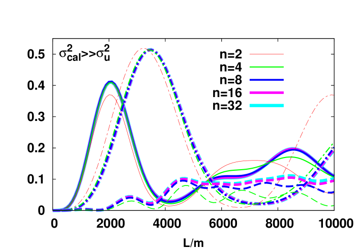
where $\epsilon(E)$, $Y(E)$, $\sigma(E)$ stand for the detection efficiency, the neutrino yield at the reactor, and the cross section, respectively. The numerical value of $D(L)$ is plotted in Fig. 1 as a function of $L$, where the reference value for $|\Delta m^{2}_{13}|$ is 2.2$\times 10^{-3}$eV² which was obtained by a combined analysis Maltoni:2004ei of the data of the atmospheric neutrino and K2K experiments. Here we assume $\sigma_{\text{u}}={\cal O}(0.1)\%$ and $\sigma_{\text{c}}={\cal O}(1)\%$.  $(4\sigma_{\text{c}}^{2}+2\sigma_{\text{u}}^{2})^{-1}$ is much smaller than $(2\sigma_{\text{u}}^{2})^{-1}$ while $D(L_{\text{F}})+D(L_{\text{N}})$ and $D(L_{\text{F}})-D(L_{\text{N}})$ are generally comparable in magnitude, so the first term in Eq. (2) can be ignored. Hence $\chi^{2}$ is given approximately by

$$\chi^{2}\simeq\sin^{4}2\theta_{13}\frac{\left[D(L_{\text{F}})-D(L_{\text{N}})\right]^{2}}{2\sigma^{2}_{\text{u}}}.$$ (3)

The hypothesis of no oscillation is excluded at the 90%CL if $\chi^{2}$ is larger than 2.7, which corresponds to the value at the 90%CL for one degree of freedom. This implies that the systematic limit on $\sin^{2}2\theta_{13}$ at the 90%CL, or the sensitivity in the limit of infinite statistics, is given by

$$\left(\sin^{2}2\theta_{13}\right)_{\text{limit}}^{\text{sys~{}only}}\simeq\sqrt{2.7}\frac{\sqrt{2}\sigma_{\text{u}}}{D(L_{\text{F}})-D(L_{\text{N}})}.$$ (4)

To optimize $\left(\sin^{2}2\theta_{13}\right)_{\text{limit}}^{\text{sys~{}only}}$, therefore, we have to minimize $D(L_{\text{N}})\equiv\langle\sin^{2}\left({\Delta m^{2}_{13}L_{\text{N}}/4E}\right)\rangle$ and maximize $D(L_{\text{F}})\equiv\langle\sin^{2}\left({\Delta m^{2}_{13}L_{\text{F}}/4E}\right)\rangle$. Since the possible maximum value of $D(L_{\text{F}})-D(L_{\text{N}})$ is 0.82, which is obtained with $L_{\text{F}}=2.0$km and $L_{\text{F}}=0$ for $|\Delta m^{2}_{13}|=2.2\times 10^{-3}\text{eV}^{2}$, the lower bound of $\left(\sin^{2}2\theta_{13}\right)_{\text{limit}}^{\text{sys~{}only}}$ in this case is estimated as:

$$\mbox{\rm lower bound of }\left(\sin^{2}2\theta_{13}\right)_{\text{limit}}^{\text{sys~{}only}}\simeq\frac{\sqrt{2.7}\sqrt{2}\sigma_{\text{u}}}{0.82}=2.8\,\sigma_{\text{u}}.$$ (5)

Eq. (5) indicates that the sensitivity is at best $\sin^{2}2\theta_{13}\simeq 0.016$ if we adopt the reference value $\sigma_{\text{u}}=0.6\%$ assumed in Ref. Minakata:2002jv . To reach this limit of the sensitivity, we have to set $L_{\text{F}}$ as close to 2.0km as possible, set $L_{\text{N}}$ as close to 0 as possible. For the case with finite statistical errors, $L_{\text{F}}$ which is slightly smaller than 2km is appropriate because it gives smaller statistical errors.

III Systematic limit of $\sin^{2}{2\theta_{13}}$ by a spectral analysis

In the previous section we have seen that the sensitivity to $\sin^{2}{2\theta_{13}}$ is governed by the uncorrelated systematic error of the detectors in the rate analysis. In this section we will examine what happens if we use spectral information also.

We introduce the systematic errors in almost the same way as in Huber:2003pm . $\chi^{2}$ is given by

$$\displaystyle\chi^{2} = \min_{\alpha^{\prime}s}\Bigg{\{}\displaystyle\sum_{A=N,F}\sum_{i=1}^{n}\frac{1}{(t^{A}_{i}\sigma^{A}_{i})^{2}}\left[m^{A}_{i}-t^{A}_{i}(1+\alpha+\alpha^{A}+\alpha_{i})-\alpha_{\text{cal}}^{A}t^{A}_{i}v^{A}_{i}\right]^{2}$$ (6)

$$+ \displaystyle\sum_{A=N,F}\left[\left(\frac{\alpha^{A}}{\sigma_{\text{dB}}}\right)^{2}+\left(\frac{\alpha_{\text{cal}}^{A}}{\sigma_{\text{cal}}}\right)^{2}\right]+\displaystyle\sum_{i=1}^{n}\left(\frac{\alpha_{i}}{\sigma_{\text{Db}}}\right)^{2}+\left(\frac{\alpha}{\sigma_{\text{DB}}}\right)^{2}\Bigg{\}}.$$

Here, $m^{A}_{i}$ is the number of events to be measured at the near ($A=N$) and far ($A=F$) for the $i$-th energy bin with the neutrino oscillation, and $t^{A}_{i}$ is the theoretical prediction without the oscillation. $(\sigma^{A}_{i})^{2}$ is the uncorrelated error which consists of the statistical plus uncorrelated bin-to-bin systematic error:

$$(t^{A}_{i}\sigma^{A}_{i})^{2}=t^{A}_{i}+\left(t^{A}_{i}\sigma^{A}_{\text{db}}\right)^{2},$$

where $\sigma^{A}_{\text{db}}$ is the uncorrelated bin-to-bin systematic error. For simplicity we assume that sizes of the bin-to-bin uncorrelated systematic errors of the detectors and of the flux are independent of the energy. This may not be the case in practical situations, but our analytic discussions will be illuminative to see how each systematic error affects the sensitivity. $\alpha$ is a variable which corresponds to a common overall normalization error $\sigma_{\text{DB}}$ for the number of events. $\alpha^{A}~{}(A=N,F)$ is a variable which introduces the detector-specific uncertainties $\sigma_{\text{dB}}$ of the near and far detectors. $\alpha_{i}~{}(i=1,\cdots,n)$ is a variable for an uncertainty $\sigma_{\text{Db}}$ of the theoretical prediction for each energy bin which is uncorrelated between different energy bins. $\alpha_{\text{cal}}^{A}~{}(A=N,F)$ is a variable which introduces an energy calibration uncertainty $\sigma_{\text{cal}}$ and comes in the theoretical prediction in the form of $(1+\alpha_{\text{cal}}^{A})E$ instead of the observed energy $E$. Thus, the deviation $v^{A}_{i}$ (divided by the expected number of events) from the theoretical prediction $t^{A}_{i}$ due to this uncertainty can be written as

$$v^{A}_{i}=\lim_{\alpha_{\text{cal}}^{A}\rightarrow 0}\frac{1}{\alpha_{\text{cal}}^{A}t^{A}_{i}}\left[\frac{N_{p}T}{4\pi L_{A}^{2}}\int_{(1+\alpha_{\text{cal}}^{A})E_{i}}^{(1+\alpha_{\text{cal}}^{A})E_{i+1}}dE\epsilon(E)Y(E)\sigma(E)-t^{A}_{i}\right],$$ (7)

where $N_{p}$ is the number of target protons in the detector, $T$ denotes the exposure time, and $L_{A}$ is the baseline for the detector $A$. We have used the definition

$$t^{A}_{i}\equiv\frac{N_{p}T}{4\pi L_{A}^{2}}\int_{E_{i}}^{E_{i+1}}dE\epsilon(E)Y(E)\sigma(E).$$ (8)

Our strategy is to assume no oscillation in the theoretical prediction $t^{A}_{i}$, to plug the number of events with oscillation in $m^{A}_{i}$, and to see the sensitivity by looking at the value of $\chi^{2}$. Since $\chi^{2}$ is quadratical in the variables $\alpha$, $\alpha^{A}$, $\alpha_{i}$, $\alpha_{\text{cal}}^{A}$, we can minimize with respect to these variables in Eq. (6) exactly. Hereafter, we take the limit of infinite statistics, i.e., $1/t^{A}_{i}\rightarrow 0$ in order to see how systematic errors affect the sensitivity to $\sin^{2}2\theta_{13}$; We refer to the sensitivity in this limit as “the systematic limit”. Since we assume no oscillation for the theoretical prediction $t^{A}_{i}$, the quantity $v^{A}_{i}$ in Eq. (7) is independent of $A(=N,F)$:

$$v^{N}_{i}=v^{F}_{i}=v_{i}.$$ (9)

After some calculations (see Appendix A for details), (6) is rewritten as

$$\chi^{2} = \frac{\sin^{4}2\theta_{13}}{2}\left\{\frac{1}{\sigma^{2}_{\text{db}}/n}\,\cdot\,\frac{1}{n}\sum_{j=1}^{n-2}\left[\vec{u}^{{}^{(-)}}_{j}\cdot(\vec{D}^{F}-\vec{D}^{N})\right]^{2}\right.$$ (10)

$$+\frac{1}{(\sigma^{2}_{\text{db}}+\Lambda^{{}^{(-)}}_{-})/n}\,\cdot\,\frac{1}{n}\left[\vec{u}^{{}^{(-)}}_{n-1}\cdot(\vec{D}^{F}-\vec{D}^{N})\right]^{2}$$

$$+\frac{1}{(\sigma^{2}_{\text{db}}+\Lambda^{{}^{(-)}}_{+})/n}\,\cdot\,\frac{1}{n}\left[\vec{u}^{{}^{(-)}}_{n}\cdot(\vec{D}^{F}-\vec{D}^{N})\right]^{2}$$

$$+\frac{1}{(\sigma^{2}_{\text{db}}+2\sigma^{2}_{\text{Db}})/n}\,\cdot\,\frac{1}{n}\sum_{j=1}^{n-2}\left[\vec{u}^{{}^{(+)}}_{j}\cdot(\vec{D}^{F}+\vec{D}^{N})\right]^{2}$$

$$+\frac{1}{(\sigma^{2}_{\text{db}}+2\sigma^{2}_{\text{Db}}+\Lambda^{{}^{(+)}}_{-})/n}\,\cdot\,\frac{1}{n}\left[\vec{u}^{{}^{(+)}}_{n-1}\cdot(\vec{D}^{F}+\vec{D}^{N})\right]^{2}$$

$$\left.+\frac{1}{(\sigma^{2}_{\text{db}}+2\sigma^{2}_{\text{Db}}+\Lambda^{{}^{(+)}}_{+})/n}\,\cdot\,\frac{1}{n}\left[\vec{u}^{{}^{(+)}}_{n}\cdot(\vec{D}^{F}+\vec{D}^{N})\right]^{2}\right\},$$

where we have introduced the variables

$$D^{A}_{i} \equiv -\frac{1}{\sin^{2}2\theta_{13}}\frac{m^{A}_{i}-t^{A}_{i}}{t^{A}_{i}}={\displaystyle\int_{E_{i}}^{E_{i+1}}dE~{}\epsilon(E)Y(E)\sigma(E)\sin^{2}\left({\Delta m^{2}_{13}L_{A}\over 4E}\right)\over\displaystyle\int_{E_{i}}^{E_{i+1}}dE~{}\epsilon(E)Y(E)\sigma(E)},$$ (11)

and $\vec{u}^{{}^{(\pm)}}_{j}$ are the orthonormal eigenvectors of some $n\times n$ unitary matrices (see Appendix A). $\Lambda^{{}^{(-)}}$ is defined by $b^{(-)}\equiv\sigma_{\text{dB}}^{2}$ and $\sigma_{\text{cal}}$ while $\Lambda^{{}^{(+)}}$ is defined by $b^{(+)}\equiv\sigma_{\text{dB}}^{2}+\sigma_{\text{DB}}^{2}$ and $\sigma_{\text{cal}}$; $\Lambda^{{}^{(-)}}$ ($\Lambda^{{}^{(+)}}$) vanishes for $b^{(-)}=0$ ($b^{(+)}=0$) or $\sigma_{\text{cal}}=0$, and then the second (fifth) term in Eq. (10) degenerate to the first (fourth) term. The first three terms in Eq. (10) correspond to the comparisons of the numbers of events at the two detectors because these terms does not include $\vec{D}^{F}+\vec{D}^{N}$ and the correlated errors between the detectors ($\sigma_{\text{Db}}$ and $\sigma_{\text{DB}}$). We see that the first and fourth terms in Eq. (10) correspond to the “pure” spectral analysis because these terms are free from $\sigma_{\text{cal}}$ and correlated errors among bins ($\sigma_{\text{dB}}$ and $\sigma_{\text{DB}}$); Other four terms include the effect of the rate analysis.

Here we will take the following assumptions for the systematic errors:

$$\sigma_{\text{db}} \lesssim \sigma_{\text{u}}={\cal O}(0.1)\%,$$

$$\sigma_{\text{dB}} \simeq \sigma_{\text{u}}={\cal O}(0.1)\%,$$

$$\sigma_{\text{Db}} \lesssim \sigma_{\text{c}}={\cal O}(1)\%,$$

$$\sigma_{\text{DB}} \simeq \sigma_{\text{c}}={\cal O}(1)\%,$$

$$\sigma_{\text{cal}} = {\cal O}(0.1)\%.$$ (12)

Roughly speaking, the errors must satisfy the relations $\sigma_{\text{u}}^{2}\simeq\sigma_{\text{dB}}^{2}+\sigma_{\text{db}}^{2}/n$ and $\sigma_{\text{c}}^{2}\simeq\sigma_{\text{DB}}^{2}+\sigma_{\text{Db}}^{2}/n$, where $\sigma_{\text{u}}$ and $\sigma_{\text{c}}$ are the errors appear in the rate analysis (2). Among the reactor experiments in the past, Bugey Declais:1994su seems to be the only experiment in which the energy spectrum analysis was performed with the identical detectors. We have learned Stutz that $\sigma_{\text{db}}$ in the Bugey experiment was of order of 0.5%. 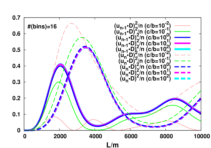We have checked numerically that each factor $\displaystyle\frac{1}{n}\sum_{j=1}^{n-2}\left[\vec{u}^{{}^{(\pm)}}_{j}\cdot(\vec{D}^{F}\pm\vec{D}^{N})\right]^{2}$, $\displaystyle\frac{1}{n}\left[\vec{u}^{{}^{(\pm)}}_{n-1}\cdot(\vec{D}^{F}\pm\vec{D}^{N})\right]^{2}$, $\displaystyle\frac{1}{n}\left[\vec{u}^{{}^{(\pm)}}_{n}\cdot(\vec{D}^{F}\pm\vec{D}^{N})\right]^{2}$ is approximately independent of the number $n$ of bins for $n\gtrsim 8$, and the maximum value of these factors range from 0.4 to 2 (See Table 1). In most of the analyses in the present paper we take the number $n$ of bins $n=16$ and the energy interval 2.8MeV$\leq E_{\nu}\leq$7.8MeV. The optimized baselines $L_{F}$ and $L_{N}$ do depend on the energy interval of the analysis because different energy interval gives different average of the neutrino energy. We adopt the energy interval 2.8MeV$\leq E_{\nu}\leq$7.8MeV because (i) the same energy interval was used in the analysis of the Bugey experiment, and (ii) the value of $\Lambda^{{}^{(-)}}_{-}/n$ becomes approximately independent of the number $n$ of bins. (ii) is not necessarily the case, for example, if we take the energy interval 1.8MeV$\leq E_{\nu}\leq$7.8MeV because in this case the value of $|\vec{v}|$ becomes so large near the threshold energy $E_{\nu}\sim 1.8$MeV that $\Lambda^{{}^{(-)}}_{-}/n$ would depend on $n$. In fact, we can neglect such an energy region near the threshold because the region has only small number of events and does not affect the value of $\chi^{2}$ so much.

From the assumed values in Eq. (12) it follows that the last three terms in Eq. (10) are negligible because the coefficients in front of these three factors are much smaller than those in front of the first three and because numerical values of the factors $\displaystyle\frac{1}{n}\sum_{j=1}^{n-2}\left[\vec{u}^{{}^{(\pm)}}_{j}\cdot(\vec{D}^{F}\pm\vec{D}^{N})\right]^{2}$, $\displaystyle\frac{1}{n}\left[\vec{u}^{{}^{(\pm)}}_{n-1}\cdot(\vec{D}^{F}\pm\vec{D}^{N})\right]^{2}$ and $\displaystyle\frac{1}{n}\left[\vec{u}^{{}^{(\pm)}}_{n}\cdot(\vec{D}^{F}\pm\vec{D}^{N})\right]^{2}$ are all comparable, as can be seen from Table 1. Furthermore, it turns out that the third term in Eq. (10) is negligible compared to the second term. This is because

$$\Lambda^{{}^{(-)}}_{-}/n\simeq 0.46\sigma^{2}_{\text{dB}}\ll\Lambda^{{}^{(-)}}_{+}/n\simeq 24\sigma^{2}_{\text{cal}}$$

are satisfied for our reference values (See Appendix C) and because the values of $\displaystyle\frac{1}{n}\left[\vec{u}^{{}^{(-)}}_{n-1}\cdot(\vec{D}^{F}-\vec{D}^{N})\right]^{2}$ and $\displaystyle\frac{1}{n}\left[\vec{u}^{{}^{(-)}}_{n}\cdot(\vec{D}^{F}-\vec{D}^{N})\right]^{2}$ are comparable. Thus we obtain

$$\chi^{2} \simeq \frac{\sin^{4}2\theta_{13}}{2}\left\{\frac{1}{\sigma^{2}_{\text{db}}/n}\,\cdot\,\frac{1}{n}\sum_{j=1}^{n-2}\left[\vec{u}^{{}^{(-)}}_{j}\cdot(\vec{D}^{F}-\vec{D}^{N})\right]^{2}\right.$$ (13)

$$\qquad\qquad+\left.\frac{1}{\sigma^{2}_{\text{db}}/n+0.46\sigma^{2}_{\text{dB}}}\,\cdot\,\frac{1}{n}\left[\vec{u}^{{}^{(-)}}_{n-1}\cdot(\vec{D}^{F}-\vec{D}^{N})\right]^{2}\right\}.$$

This is the main result of this paper and is to be compared with the result (3) by the rate analysis. Once the baselines $L_{F}$ and $L_{N}$ are given, then (13) contains only $\sigma^{2}_{\text{db}}/\sqrt{n}$ and $\sigma^{2}_{\text{dB}}$ as the parameters because the coefficients $\displaystyle\frac{1}{n}\sum_{j=1}^{n-2}\left[\vec{u}^{{}^{(-)}}_{j}\cdot(\vec{D}^{F}-\vec{D}^{N})\right]^{2}$ and $\displaystyle\frac{1}{n}\left[\vec{u}^{{}^{(-)}}_{n-1}\cdot(\vec{D}^{F}-\vec{D}^{N})\right]^{2}$ are almost independent of $n$. These coefficients seem to give good measures for the potential of an experiment in spectral analysis almost independently of $n$ and the sizes of errors; The larger values of these measures means the better setup in principle.

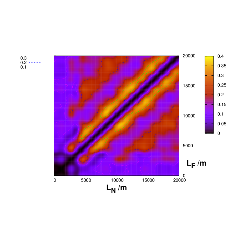
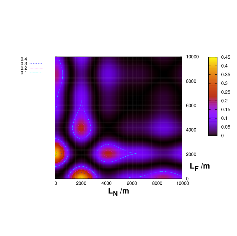
From numerical calculations we find that the dependence of the first term in Eq. (13) on $L_{F}$ and $L_{N}$ is quite different from that of the second term and the values of $\displaystyle\frac{1}{n}\sum_{j=1}^{n-2}\left[\vec{u}^{{}^{(-)}}_{j}\cdot(\vec{D}^{F}-\vec{D}^{N})\right]^{2}$ and $\displaystyle\frac{1}{n}\left[\vec{u}^{{}^{(-)}}_{n-1}\cdot(\vec{D}^{F}-\vec{D}^{N})\right]^{2}$ are plotted as functions of $L_{F}$ and $L_{N}$ in Figs. 4 and 5. $\displaystyle\frac{1}{n}\sum_{j=1}^{n-2}\left[\vec{u}^{{}^{(-)}}_{j}\cdot(\vec{D}^{F}-\vec{D}^{N})\right]^{2}$ of the first term in Eq. (13) has the maximum value 0.37 at $L_{F}=$10.6km and $L_{N}$=8.4km, while $\displaystyle\frac{1}{n}\left[\vec{u}^{{}^{(-)}}_{n-1}\cdot(\vec{D}^{F}-\vec{D}^{N})\right]^{2}$ of the second is extremely small for these baselines. Theoretically, therefore, the first term is optimized for $L_{F}=$10.6km and $L_{N}$=8.4km. In this case the sensitivity to $\sin^{2}2\theta_{13}$ in the limit of infinite statistics is given by

$$\left(\sin^{2}2\theta_{13}\right)_{\text{limit}}^{\text{sys~{}only}} \simeq \sqrt{\frac{\left.\chi^{2}\right|_{\text{90\%CL}}\times 2}{0.37}}\,\frac{\sigma_{\text{db}}}{\sqrt{n}}=\sqrt{\frac{2.7\times 2}{0.37}}\,\frac{\sigma_{\text{db}}}{\sqrt{n}}=3.8\frac{\sigma_{\text{db}}}{\sqrt{n}}$$

$$\mbox{\rm for}~{}L_{F}=10.6\mbox{\rm km~{}and~{}}L_{N}=8.4\mbox{\rm km}.$$

If $\sigma_{\text{db}}/\sqrt{n}$ is smaller than $\sigma_{\text{u}}$, the sensitivity (III) of the spectral analysis is better than (5) of the rate analysis. It should be noted, however, that this sensitivity is attained only if the statistical error in each bin becomes negligible compared to the systematic errors which are already assumed to be smaller than ${\cal O}(0.1)\%$. In order for this to happen at $L_{F}=$10km, we would need at least 100 kton$\cdot$yr even at the Kashiwazaki-Kariwa nuclear power plant, so the optimization of the first term in (13), namely the optimization of the spectral analysis, is not realistic for the investigation of the oscillation of $|\Delta m^{2}_{13}|={\cal O}(10^{-3})\text{eV}^{2}$.

Next, we consider to optimize the the second term in Eq. (13), i.e. the term which roughly corresponds to the rate analysis. This is achieved at $L_{F}=$2.1km and $L_{N}$=0km. For these values of the baselines, Eq. (13) becomes numerically

$$\chi^{2} \simeq \frac{\sin^{4}2\theta_{13}}{2}\left(\frac{3.7\times 10^{-3}}{\sigma^{2}_{\text{db}}/n}+\frac{4.1\times 10^{-1}}{\sigma^{2}_{\text{db}}/n+0.46\sigma^{2}_{\text{dB}}}\right)$$

$$\mbox{\rm for}~{}L_{F}=2.1\mbox{\rm km~{}and~{}}L_{N}=0\mbox{\rm km}.$$

If $\sigma^{2}_{\text{db}}/n\gg(1/100)\sigma^{2}_{\text{dB}}$ then the second term on the right-hand side in Eq. (III) is dominant. In this case, the sensitivity is not so much different from that in rate analysis because the second term is understood as a rate-like one. On the other hand, if $\sigma^{2}_{\text{db}}/n\ll(1/100)\sigma^{2}_{\text{dB}}$ then the first term in Eq. (III) dominates the sensitivity, and it is given by

$$\left(\sin^{2}2\theta_{13}\right)_{\text{limit}}^{\text{sys~{}only}} \sim \sqrt{\frac{2.7\times 2}{3.7\times 10^{-3}}}\,\frac{\sigma_{\text{db}}}{\sqrt{n}}=37\frac{\sigma_{\text{db}}}{\sqrt{n}}$$

$$\mbox{\rm if}~{}\frac{\sigma^{2}_{\text{db}}}{n}\ll\frac{1}{100}\sigma^{2}_{\text{dB}}\simeq\frac{1}{100}\sigma_{\text{u}}^{2}\simeq{\cal O}\left((0.01\%)^{2}\right).$$

Since the coefficient $4.1\times 10^{-1}$ of the second term in (III) is much larger than the coefficient $3.7\times 10^{-3}$ of the first term, $\sigma_{\text{db}}/\sqrt{n}$ must be much smaller than $\sigma_{\text{u}}$ in order to use (III) and to improve the sensitivity significantly beyond the one in the rate analysis . If the setup is optimized for the rate analysis, therefore, it is not easy for the spectral analysis to give us much better sensitivity than what the rate analysis does. On the other hand, since the difference between the coefficients of the first and second terms in (III) can be smaller for the setup which deviates from the optimal one for the rate analysis, the spectral analysis could compensate the loss of the sensitivity due to the deviation.

To illustrate the usefulness of the formula (13), let us see if it reproduces the result in Huber:2003pm , where the number $n$ of the energy bins was assumed to be 62, the energy interval was 1.8MeV$\leq E_{\nu}\leq$8.0MeV, $L_{F}$=1.7km, $L_{N}$=0.17km, and the reference values are $|\Delta m^{2}_{31}|=3.0\times 10^{-3}$eV², $\sigma_{\text{dB}}$=0.6%, and $\sigma_{\text{db}}$=0.1% (the most optimistic case in Huber:2003pm ). We found from numerical calculations that if we perform the spectrum analysis with the energy interval 1.8MeV$\leq E_{\nu}\leq$8.0MeV, the number $n$=62 of bins, the baselines $L_{F}$=1.7km and $L_{N}$=0.17km, then Eq. (13) is modified for $|\Delta m^{2}_{31}|=3.0\times 10^{-3}$eV² as

$$\chi^{2} \simeq \frac{\sin^{4}2\theta_{13}}{2}\left(\frac{6.8\times 10^{-2}}{\sigma^{2}_{\text{db}}/62}+\frac{3.3\times 10^{-1}}{\sigma^{2}_{\text{db}}/62+0.95\sigma^{2}_{\text{dB}}}\right)$$

$$\mbox{\rm for}~{}L_{F}=1.7\mbox{\rm km~{}and~{}}L_{N}=0.17\mbox{\rm km},$$

where we have used the fact $\vec{v}^{2}/n=1.2\times 10^{3}$ and $\vec{v}\cdot\vec{h}/n=-7.7$ for 1.8MeV$\leq E_{\nu}\leq$8.0MeV and $n$=62 to derive the factor 0.95. Note that the ratio of the coefficient 0.068 of the first term to that 0.33 of the second term is bigger than that in Eq. (III) because $L_{F}$=1.7km is longer than the optimized baseline $L\simeq$1.4km for the rate analysis in the case of $|\Delta m^{2}_{31}|=3.0\times 10^{-3}$eV². This can be seen from Fig. 2, where the value of $\displaystyle\frac{1}{n}\sum_{j=1}^{n-2}\left[\vec{u}^{{}^{(-)}}_{j}\cdot(\vec{D}^{F}-\vec{D}^{N})\right]^{2}$ increases for $L$ larger than the optimized baseline ($\simeq$2km) for the rate analysis, i.e. the baseline which optimizes $\displaystyle\frac{1}{n}\left[\vec{u}^{{}^{(-)}}_{n-1}\cdot(\vec{D}^{F}-\vec{D}^{N})\right]^{2}$, in the case of $|\Delta m^{2}_{31}|=2.2\times 10^{-3}$eV². Substituting the reference values $\sigma_{\text{dB}}$=0.6%, $\sigma_{\text{db}}$=0.1% in Eq. (III) and the value 2.7 of $\chi^{2}$ at the 90%CL for one degree of freedom, we have

$$2.7 \simeq \frac{\left(\sin^{2}2\theta_{13}\right)_{\text{limit}}^{\text{sys~{}only}}}{2}\left(\frac{6.8\times 10^{-2}\times 62}{10^{-6}}+\frac{0.33}{0.95\times(6\times 10^{-3})^{2}}\right)$$

$$\simeq 4.2\times 10^{6}\times\frac{\left(\sin^{2}2\theta_{13}\right)_{\text{limit}}^{\text{sys~{}only}}}{2}$$

which gives

$$\left(\sin^{2}2\theta_{13}\right)_{\text{limit}}^{\text{sys~{}only}}\simeq\sqrt{\frac{5.4}{4.2}}\times 10^{-3}\sim 1\times 10^{-3}.$$

This is almost consistent with the result in Huber:2003pm . From this calculation it is obvious that such a good sensitivity was obtained in Huber:2003pm because the uncorrelated bin-to-bin systematic error $\sigma_{\text{db}}$ was assumed to be very small and the number of bins was large.

IV Oscillation experiments for $\Delta m^{2}\sim{\cal O}(1)$eV²

In the previous section, in the case of reactor experiments to measure $\sin^{2}2\theta_{13}$ for $\Delta m^{2}\sim{\cal O}(10^{-3})$eV², we have seen that the optimal baseline lengths for the spectral analysis are very long and it is not a realistic idea to accumulate large number of events at such baselines. If we want to observe neutrino oscillations for $\Delta m^{2}\sim{\cal O}(1)$eV², however, the optimal setup for the spectral analysis becomes realistic. With the standard three flavor scenario, there is little motivation to look for neutrino oscillations for $\Delta m^{2}\sim{\cal O}(1)$eV², but if we consider more general frameworks with sterile neutrinos then oscillations with $\Delta m^{2}\sim{\cal O}(1)$eV² are still possible. In this section we briefly discuss such a possibility for the sake of completeness.

In ref. Sorel:2003hf it was shown that the scheme with two sterile neutrinos is still consistent with all the data, and the best fit values for $\Delta m^{2}_{14}$ and $\sin^{2}2\theta_{14}$ are 0.9eV² and 0.058. $\Delta m^{2}$=0.9eV² is the value for which the hypothesis for neutrino oscillations is excluded only weakly by the Bugey experiment Declais:1994su . If the (3+2)–scheme is realized by Nature, therefore, we should be able to observe neutrino oscillation at $\Delta m^{2}\simeq$0.9eV². By rescaling the baselines used in (III) by $2.2\times 10^{-3}$eV²/0.9eV${}^{2}\simeq 1/410$, we see in the limit of infinite statistics that the optimum set of baselines for $\Delta m^{2}=0.9$eV² is

$$L_{F}=26\text{m},~{}~{}L_{N}=21\text{m}.$$

If we put the two detectors with this set of baselines, then in the limit of infinite statistics, assuming the number of bins $n=25$, the bin-to-bin uncorrelated systematic error $\sigma_{\text{db}}$=0.5% and the mixing angle $\sin^{2}2\theta=0.058$, we could have

$$\chi^{2}\simeq\frac{\sin^{4}2\theta}{2}\cdot\frac{0.37}{(5\times 10^{-3})^{2}/25}\simeq 6\times 10^{2}.$$ (18)

Eq. (18) would imply that neutrino oscillation for $\Delta m^{2}\simeq$0.9eV² can be established with tremendous significance. This result is to be compared to the rate analysis with (3), where the set of optimum baselines for $\Delta m^{2}\simeq$0.9eV² would be

$$L_{F}=5\text{m},~{}~{}L_{N}=0\text{m}.$$ (19)

Assuming that these baselines are technically possible, $\chi^{2}$ at $\sin^{2}2\theta=0.058$ would be

$$\chi^{2}\simeq\frac{\sin^{4}2\theta}{2}\cdot\frac{0.82}{(0.6\times 10^{-2})^{2}}\simeq 4\times 10^{1}.$$ (20)

From practical point of view, however, Eq. (19) would imply that both the detectors be placed inside of the reactor and Eq. (19) is not realistic. The value of $\chi^{2}$ would be smaller than Eq. (20) and much smaller than Eq. (18). Thus, the spectral analysis is much more advantageous than the rate analysis in search of neutrino oscillations for $\Delta m^{2}\sim{\cal O}(1)$eV².

V Discussion and Conclusion

We applied our analytical method to estimate the sensitivity to $\sin^{2}2\theta$ in the limit of infinite statistics, which we refer to as “the systematic limit”, in the spectral analysis at a reactor neutrino oscillation experiment with one reactor and two detectors. In a rate analysis, the systematic limit (4) is set by the the uncorrelated systematic error $\sigma_{\text{u}}$ of the detectors, and is given by 2.8$\sigma_{\text{u}}$ Sugiyama:2004bv . In a spectrum analysis, we derived an analogous formula for $\chi^{2}$ which gives the systematic limit. The formula for $\chi^{2}$ contains two terms which could potentially dominate $\chi^{2}$ (13). One is the contribution from the bin-to-bin correlated detector specific systematic error $\sigma_{\text{dB}}$ and the other is the one from $\sigma_{\text{db}}/\sqrt{n}$ which is the uncorrelated bin-to-bin systematic error divided by the square-root of the number $n$ of bins. The optimal setup for the spectral analysis is found to be unrealistic for $\Delta m^{2}={\cal O}(10^{-3})\text{eV}^{2}$ because the optimal baselines are too long to accumulate large number of events. The optimization can be realistic, however, for $\Delta m^{2}={\cal O}(1)\text{eV}^{2}$ to search for sterile neutrino oscillations. If the baselines are optimized for the rate analysis, the improvement of the sensitivity with the spectral analysis is not significant in most cases. On the other hand, the spectral analysis can be effective for the experiment whose setup deviates from the optimal one for the rate analysis. For example, the spectral analysis could compensate the disadvantage of the rate analysis in the KASKA experiment which has near detectors with relatively long baselines ($\sim$ 300–400m), or that in the DCHOOZ experiment that has a far detector at a distance ($\simeq 1$km) shorter than the optimal one for the rate analysis. In any case, it is very important in the future reactor experiments to estimate $\sigma_{\text{dB}}$ and especially $\sigma_{\text{db}}$.

Appendix A Derivation of the covariance matrix

After taking the limit $1/t^{A}_{i}\rightarrow 0$ of infinite statistics, Eq. (6) becomes

$$\displaystyle\chi^{2} = \min_{\alpha^{\prime}s}\Bigg{\{}\displaystyle\sum_{A=N,F}\sum_{i=1}^{n}\frac{\left(m^{A}_{i}/t^{A}_{i}-1-\alpha-\alpha^{A}-\alpha_{i}-\alpha_{\text{cal}}^{A}v^{A}_{i}\right)^{2}}{(\sigma^{A}_{\text{db}})^{2}}$$

$$+ \displaystyle\sum_{A=N,F}\left[\left(\frac{\alpha^{A}}{\sigma_{\text{dB}}}\right)^{2}+\left(\frac{\alpha_{\text{cal}}^{A}}{\sigma_{\text{cal}}}\right)^{2}\right]+\displaystyle\sum_{i=1}^{n}\left(\frac{\alpha_{i}}{\sigma_{\text{Db}}}\right)^{2}+\left(\frac{\alpha}{\sigma_{\text{DB}}}\right)^{2}\Bigg{\}}$$

$$\equiv \min_{\alpha^{\prime}s}\chi^{2}_{\alpha}.$$

Let us redefine the variables

$$y^{A}_{i} \equiv \frac{m^{A}_{i}-t^{A}_{i}}{t^{A}_{i}}=-\sin^{2}2\theta_{13}D^{A}_{i}$$

and let us introduce a vector notation

$$\vec{y}^{N}\equiv\left(\begin{array}[]{c}y^{N}_{1}\\ \vdots\\ y^{N}_{n}\end{array}\right),\qquad\vec{y}^{F}\equiv\left(\begin{array}[]{c}y^{F}_{1}\\ \vdots\\ y^{F}_{n}\end{array}\right).$$ (27)

Following the discussions in the Appendix A in Sugiyama:2004bv , the matrix element of the covariance matrix can be obtained as the expectation value of $y^{A}_{i}\,y^{B}_{j}$:

$$\left(\rho\right)^{AB}_{ij} = \left\langle y^{A}_{i}y^{B}_{j}\right\rangle$$

$$\equiv {\cal N}\int d\alpha\prod_{A=N,F}\int d\vec{y}^{A}\int d\alpha^{A}\int d\alpha_{\text{cal}}^{A}\prod_{i=1}^{n}\int d\alpha_{i}~{}y^{A}_{i}\,y^{B}_{j}\,\exp\left(-\frac{\chi^{2}_{\alpha}}{2}\right),$$

where the normalization ${\cal N}$ is defined in such a way that $\langle 1\rangle=1$. From a straightforward calculation, we have

$$\left\langle y^{A}_{i}y^{B}_{j}\right\rangle = \delta^{AB}\delta_{ij}\,\sigma_{\text{db}}^{2}+\sigma_{\text{DB}}^{2}+\delta^{AB}\,\sigma_{\text{dB}}^{2}+\delta_{ij}\,\sigma_{\text{Db}}^{2}+\delta^{AB}v^{A}_{i}v^{A}_{j}\,\sigma^{2}_{\text{cal}}.$$

Thus we have

$$\displaystyle\chi^{2}=\left(\begin{array}[]{ll}\vec{y}^{N\ T},&\vec{y}^{F\ T}\end{array}\right)\rho^{-1}\left(\begin{array}[]{l}\vec{y}^{N}\\ \vec{y}^{F}\end{array}\right)=\sin^{4}2\theta_{13}\left(\begin{array}[]{ll}\vec{D}^{N\ T},&\vec{D}^{F\ T}\end{array}\right)\rho^{-1}\left(\begin{array}[]{l}\vec{D}^{N}\\ \vec{D}^{F}\end{array}\right),$$ (34)

where the covariance matrix $\rho$ is defined by

$$\rho=\left(\begin{array}[]{ll}M&N\\ N&M\end{array}\right),$$ (37)

with

$$M \equiv \left(\sigma^{2}_{\text{Db}}+\sigma^{2}_{\text{db}}\right)I_{n}+\left(\sigma^{2}_{\text{DB}}+\sigma^{2}_{\text{dB}}\right)H_{n}+\sigma^{2}_{\text{cal}}G_{n},$$

$$N \equiv \sigma^{2}_{\text{Db}}I_{n}+\sigma^{2}_{\text{DB}}H_{n}.$$ (38)

Here $I_{n}$ is an $n\times n$ unit matrix, $H_{n}$ and $G_{n}$ are $n\times n$ matrices defined by

$$H_{n} \equiv \left(\begin{array}[]{ccc}1&\cdots&1\\ \vdots&&\vdots\\ 1&\cdots&1\end{array}\right),$$ (42)

$$G_{n} \equiv \left(\begin{array}[]{cccc}v_{1}^{2}&v_{1}v_{2}&\cdots&v_{1}v_{n}\\ v_{1}v_{2}&v_{2}^{2}&\cdots&v_{2}v_{n}\\ \vdots&\vdots&&\vdots\\ v_{1}v_{n}&v_{2}v_{n}&\cdots&v_{n}^{2}\end{array}\right),$$ (47)

where $v_{j}~{}(j=1,\cdots,n)$ is defined by Eqs. (7), and (9). Note that the covariance matrix does not include oscillation parameters but only errors. Diagonalization of the covariance matrix is useful to see which errors dominate $\chi^{2}$.

Now (37) can be cast into a block diagonal by

$$\left(\begin{array}[]{ll}M&N\\ N&M\end{array}\right)=\frac{1}{2}\left(\begin{array}[]{rr}I_{n}&-I_{n}\\ I_{n}&I_{n}\end{array}\right)\left(\begin{array}[]{cc}M+N&0\\ 0&M-N\end{array}\right)\left(\begin{array}[]{rr}I_{n}&I_{n}\\ -I_{n}&I_{n}\end{array}\right).$$ (56)

We obtain

$$\chi^{2}=\frac{\sin^{4}2\theta_{13}}{2}\left(\begin{array}[]{ll}\vec{D}^{F\ T}+\vec{D}^{N\ T},&\vec{D}^{F\ T}-\vec{D}^{N\ T}\end{array}\right)\left(\begin{array}[]{cc}M+N&0\\ 0&M-N\end{array}\right)^{-1}\left(\begin{array}[]{l}\vec{D}^{F}+\vec{D}^{N}\\ \vec{D}^{F}-\vec{D}^{N}\end{array}\right).$$ (62)

We can formally diagonalize the symmetric matrices $M+N$ and $M-N$ assuming the existence of $(n-2)$ orthonormal eigenvectors which are orthogonal to $\vec{v}$ and $\vec{h}\equiv\left(1,\cdots,1\right)^{T}$. This is described in Appendix B. Now $M+N$ and $M-N$ are diagonalized by the orthogonal matrices $U^{{}^{(+)}}$ and $U^{{}^{(-)}}$:

$$M+N = U^{{}^{(+)}}{\cal D}^{{}^{(+)}}U^{{}^{(+)}\ T},$$

$$M-N = U^{{}^{(-)}}{\cal D}^{{}^{(-)}}U^{{}^{(-)}\ T},$$ (63)

where

$${\cal D}^{{}^{(\pm)}}\equiv\mbox{\rm diag}\left(\lambda^{{}^{(\pm)}}_{1},\cdots,\lambda^{{}^{(\pm)}}_{n}\right)$$

and $\lambda^{{}^{(\pm)}}_{j}$ are the eigenvalues of $M\pm N$. From (62) and (63) we obtain

$$\chi^{2} = \frac{\sin^{4}2\theta_{13}}{2}\left(\begin{array}[]{ll}(\vec{D}^{F\ T}+\vec{D}^{N\ T})U^{{}^{(+)}},&(\vec{D}^{F\ T}-\vec{D}^{N\ T})U^{{}^{(-)}}\end{array}\right)$$ (65)

$$\times\left(\begin{array}[]{cc}{\cal D}^{{}^{(+)}}&0\\ 0&{\cal D}^{{}^{(-)}}\end{array}\right)^{-1}\left(\begin{array}[]{l}U^{{}^{(+)}\ T}(\vec{D}^{F}+\vec{D}^{N})\\ U^{{}^{(-)}\ T}(\vec{D}^{F}-\vec{D}^{N})\end{array}\right)$$

$$= \frac{\sin^{4}2\theta_{13}}{2}\left\{\sum_{j=1}^{n}\frac{\left[\vec{u}^{{}^{(+)}}_{j}\cdot(\vec{D}^{F}+\vec{D}^{N})\right]^{2}}{\lambda^{{}^{(+)}}_{j}}+\sum_{j=1}^{n}\frac{\left[\vec{u}^{{}^{(-)}}_{j}\cdot(\vec{D}^{F}-\vec{D}^{N})\right]^{2}}{\lambda^{{}^{(-)}}_{j}}\right\},$$

where $\vec{u}^{{}^{(\pm)}}_{j}$ are the orthonormal eigenvectors which appear in $U^{{}^{(\pm)}}$:

$$U^{{}^{(\pm)}}\equiv\left(\vec{u}^{{}^{(\pm)}}_{1},\cdots,\vec{u}^{{}^{(\pm)}}_{n}\right).$$

Putting

$$M\pm N \equiv a^{{}^{(\pm)}}I_{n}+b^{{}^{(\pm)}}H_{n}+cG_{n},$$

we have from (38)

$$a^{{}^{(+)}} = \sigma^{2}_{\text{db}}+2\sigma^{2}_{\text{Db}},$$

$$b^{{}^{(+)}} = \sigma^{2}_{\text{dB}}+2\sigma^{2}_{\text{DB}},$$

$$a^{{}^{(-)}} = \sigma^{2}_{\text{db}},$$

$$b^{{}^{(-)}} = \sigma^{2}_{\text{dB}},$$

$$c = \sigma^{2}_{\text{cal}}.$$

We will see in Appendix B that $\lambda^{{}^{(\pm)}}_{j}$ are given by

$$\lambda^{{}^{(+)}}_{j} = \left\{\begin{array}[]{l}a^{{}^{(+)}}\qquad\qquad\quad(j=1,\cdots,n-2)\\ a^{{}^{(+)}}+\Lambda^{{}^{(+)}}_{-}\qquad(j=n-1)\\ a^{{}^{(+)}}+\Lambda^{{}^{(+)}}_{+}\qquad(j=n)\end{array},\right.$$ (74)

$$\lambda^{{}^{(-)}}_{j} = \left\{\begin{array}[]{l}a^{{}^{(-)}}\qquad\qquad\quad(j=1,\cdots,n-2)\\ a^{{}^{(-)}}+\Lambda^{{}^{(-)}}_{-}\qquad(j=n-1)\\ a^{{}^{(-)}}+\Lambda^{{}^{(-)}}_{+}\qquad(j=n)\end{array},\right.$$ (78)

where $\Lambda^{{}^{(\pm)}}_{\pm}$ are given by

$$\Lambda^{{}^{(+)}}_{\pm}\equiv\frac{b^{{}^{(+)}}n+c\,\vec{v}^{2}}{2}\pm\sqrt{\left(\frac{b^{{}^{(+)}}n-c\,\vec{v}^{2}}{2}\right)^{2}+b^{{}^{(+)}}c\left(\vec{v}\cdot\vec{h}\right)^{2}},$$

$$\Lambda^{{}^{(-)}}_{\pm}\equiv\frac{b^{{}^{(-)}}n+c\,\vec{v}^{2}}{2}\pm\sqrt{\left(\frac{b^{{}^{(-)}}n-c\,\vec{v}^{2}}{2}\right)^{2}+b^{{}^{(-)}}c\left(\vec{v}\cdot\vec{h}\right)^{2}}.$$

Hence we obtain the $\chi^{2}$ (10). In Appendix C we will see that $\Lambda^{{}^{(\pm)}}_{\pm}/n$ are approximately independent of the number $n$ of bins for the energy interval 2.8MeV$\leq E_{\nu}\leq$7.8MeV.

Appendix B Diagonalization of the $n\times n$ matrix

In this appendix we show how we diagonalize the matrix

$$aI_{n}+bH_{n}+cG_{n},$$

where $I_{n}$ is the $n\times n$ unit matrix, and $H_{n}$, $G_{n}$ and $v_{j}$ are given by Eqs. (42), (47) and Eq. (7), respectively. Since $aI_{n}$ only shifts each eigenvalue by $a$, we will discuss the diagonalization of $bH_{n}+cG_{n}$ here. Let us introduce the notation

$$\vec{h}\equiv\left(\begin{array}[]{c}1\\ \vdots\\ 1\end{array}\right).$$ (82)

When $\vec{h}\cdot\vec{v}\neq 0$, which is satisfied in the present case for Eq. (7), we can always find in $n$-dimensional Euclidean space $n-2$ orthonormal eigenvectors $\vec{u}_{j}~{}(j=1,\cdots,n-2)$ which are orthogonal to $\vec{h}$ and $\vec{v}$, i.e.,

$$\vec{h}\cdot\vec{u}_{j}=\vec{v}\cdot\vec{u}_{j}=0\qquad(j=1,\cdots,n-2).$$ (83)

From Eq. (83) we have

$$H_{n}\vec{u}_{j}=\vec{u}_{j}\cdot\vec{h}\left(\begin{array}[]{c}1\\ \vdots\\ 1\end{array}\right)=0,$$ (87)

$$G_{n}\vec{u}_{j}=\vec{u}_{j}\cdot\vec{v}\left(\begin{array}[]{c}v_{1}\\ \vdots\\ v_{n}\end{array}\right)=0.$$ (91)

Eq. (91) indicates that $\vec{u}_{j}~{}(j=1,\cdots,n-2)$ are the $n-2$ eigenvectors of $bH_{n}+cG_{n}$ with the eigenvalue 0:

$$\left(bH_{n}+cG_{n}\right)\vec{u}_{j}=0\qquad(j=1,\cdots,n-2).$$

It turns out that the remaining 2 eigenvectors can be constructed out of $\vec{h}$ and $\vec{v}$. Straightforward calculations show the following:

$$H_{n}\vec{h}=n\vec{h},$$

$$G_{n}\vec{h}=(\vec{v}\cdot\vec{h})\vec{v},$$

$$H_{n}\vec{v}=(\vec{v}\cdot\vec{h})\vec{h},$$

$$G_{n}\vec{v}=(\vec{v}^{2})\vec{v}.$$

Hence we obtain

$$\left(bH_{n}+cG_{n}\right)\left(\begin{array}[]{c}\vec{h}\\ \vec{v}\end{array}\right)=\left(\begin{array}[]{cc}bn&c\,\vec{v}\cdot\vec{h}\\ b\vec{v}\cdot\vec{h}&c\,\vec{v}^{2}\end{array}\right)\left(\begin{array}[]{c}\vec{h}\\ \vec{v}\end{array}\right).$$ (98)

This suggests that multiplication of the vectors $\sqrt{b}\,\vec{h}$ and $\sqrt{c}\,\vec{v}$ by $bH_{n}+cG_{n}$ give the symmetric matrix

$$\left(bH_{n}+cG_{n}\right)\left(\begin{array}[]{c}\sqrt{b}\,\vec{h}\\ \sqrt{c}\,\vec{v}\end{array}\right)=\left(\begin{array}[]{cc}bn&\sqrt{bc}\,\vec{v}\cdot\vec{h}\\ \sqrt{bc}\,\vec{v}\cdot\vec{h}&c\,\vec{v}^{2}\end{array}\right)\left(\begin{array}[]{c}\sqrt{b}\,\vec{h}\\ \sqrt{c}\,\vec{v}\end{array}\right).$$ (105)

The symmetric matrix on the right-hand side can be diagonalized as

$$\left(\begin{array}[]{cc}bn&\sqrt{bc}\,\vec{v}\cdot\vec{h}\\ \sqrt{bc}\,\vec{v}\cdot\vec{h}&c\,\vec{v}^{2}\end{array}\right)=\left(\begin{array}[]{cc}\cos\psi&-\sin\psi\\ \sin\psi&\cos\psi\end{array}\right)\left(\begin{array}[]{cc}\Lambda_{+}&0\\ 0&\Lambda_{-}\end{array}\right)\left(\begin{array}[]{cc}\cos\psi&\sin\psi\\ -\sin\psi&\cos\psi\end{array}\right),$$ (114)

where $\psi$ is given by

$$\tan 2\psi\equiv\frac{\sqrt{bc}\,\vec{v}\cdot\vec{h}}{\left(bn-c\,\vec{v}^{2}\right)/2}$$ (115)

and the eigenvalues $\Lambda_{\pm}$ are

$$\Lambda_{\pm}\equiv\frac{bn+c\,\vec{v}^{2}}{2}\pm\sqrt{\left(\frac{bn-c\,\vec{v}^{2}}{2}\right)^{2}+\left(\sqrt{bc}\,\vec{v}\cdot\vec{h}\right)^{2}}.$$ (116)

Therefore, if we define

$$\left(\begin{array}[]{c}\vec{w}_{1}\\ \vec{w}_{2}\end{array}\right)\equiv\left(\begin{array}[]{cc}\cos\psi&\sin\psi\\ -\sin\psi&\cos\psi\end{array}\right)\left(\begin{array}[]{c}\sqrt{b}\,\vec{h}\\ \sqrt{c}\,\vec{v}\end{array}\right),$$ (123)

then from Eq. (105) we have

$$\left(bH_{n}+cG_{n}\right)\left(\begin{array}[]{c}\vec{w}_{1}\\ \vec{w}_{2}\end{array}\right)=\left(\begin{array}[]{cc}\Lambda_{+}&0\\ 0&\Lambda_{-}\end{array}\right)\left(\begin{array}[]{c}\vec{w}_{1}\\ \vec{w}_{2}\end{array}\right).$$ (130)

It is easy to show that the normalizations of $\vec{w}_{1}$ and $\vec{w}_{2}$ are $\sqrt{\Lambda}_{+}$ and $\sqrt{\Lambda}_{-}$, respectively. We see that the $(n-1)$-th and the $n$-th orthonormal eigenvectors are given by

$$\left(\begin{array}[]{c}\vec{u}_{n-1}\\ \vec{u}_{n}\end{array}\right)\equiv\left(\begin{array}[]{c}\vec{w}_{2}/\sqrt{\Lambda_{-}}\\ \vec{w}_{1}/\sqrt{\Lambda_{+}}\end{array}\right)=\left(\begin{array}[]{c}\displaystyle\frac{1}{\sqrt{\Lambda_{-}}}\left(-\sqrt{b}\,\vec{h}\sin\psi+\sqrt{c}\,\vec{v}\cos\psi\right)\\ \displaystyle\frac{1}{\sqrt{\Lambda_{+}}}\left(\sqrt{b}\,\vec{h}\cos\psi+\sqrt{c}\,\vec{v}\sin\psi\right)\end{array}\right)$$ (137)

with the eigenvalues $\Lambda_{-}$ and $\Lambda_{+}$.

We note in passing that (137) has the correct behaviors in the limit $b\ll c$ or $b\gg c$. In the limit $b\ll c$ we have

$$\left(\begin{array}[]{c}\vec{u}_{n-1}\\ \vec{u}_{n}\end{array}\right)\rightarrow\left(\begin{array}[]{c}\displaystyle-\frac{\vec{h}-(\vec{v}\cdot\vec{h})\vec{v}/\vec{v}^{2}}{\sqrt{n-(\vec{v}\cdot\vec{h})^{2}/\vec{v}^{2}}}\\ \displaystyle\frac{\vec{v}}{\sqrt{\vec{v}^{2}}}\end{array}\right)$$ (142)

with

$$\left(\begin{array}[]{c}\Lambda_{-}\\ \Lambda_{+}\end{array}\right)\rightarrow\left(\begin{array}[]{c}\displaystyle b\left[n-\frac{(\vec{v}\cdot\vec{h})^{2}}{\vec{v}^{2}}\right]\\ \displaystyle c\,\vec{v}^{2}\end{array}\right),$$ (147)

while in the limit $b\gg c$ we obtain

$$\left(\begin{array}[]{c}\vec{u}_{n-1}\\ \vec{u}_{n}\end{array}\right)\rightarrow\left(\begin{array}[]{c}\displaystyle\frac{\vec{v}-(\vec{v}\cdot\vec{h})\vec{h}/n}{\sqrt{\vec{v}^{2}-(\vec{v}\cdot\vec{h})^{2}/n}}\\ \displaystyle\frac{\vec{h}}{\sqrt{n}}\end{array}\right)$$ (152)

with

$$\left(\begin{array}[]{c}\Lambda_{-}\\ \Lambda_{+}\end{array}\right)\rightarrow\left(\begin{array}[]{c}\displaystyle c\left[\vec{v}^{2}-\frac{(\vec{v}\cdot\vec{h})^{2}}{n}\right]\\ \displaystyle bn\end{array}\right).$$ (157)

Putting everything together, we obtain

$$U^{T}\left(bH_{n}+cG_{n}\right)U=\mbox{\rm diag}(0,\cdots,0,\Lambda_{-},\Lambda_{+})$$ (158)

with

$$U=\left(\vec{u}_{1},\cdots,\vec{u}_{n}\right),$$

where $\vec{u}_{1},\cdots,\vec{u}_{n-2}$ are $n-2$ orthonormal vectors which are orthogonal to $\vec{v}$ and $\vec{h}$, $\vec{u}_{n-1}$ and $\vec{u}_{n}$ are given by Eq. (137), $\Lambda_{-}$ and $\Lambda_{+}$ are given by Eq. (116). Adding the unit matrix $aI_{n}$ to Eq. (158), we finally obtain

$$U^{T}\left(aI_{n}+bH_{n}+cG_{n}\right)U=\mbox{\rm diag}(a,\cdots,a,a+\Lambda_{-},a+\Lambda_{+}).$$

Appendix C The properties of $\vec{v}$

From numerical calculations, we find for $n\gtrsim 8$ and for 2.8MeV$\leq E_{\nu}\leq$7.8MeV that

$$\frac{1}{n}\vec{v}\cdot\vec{h} \simeq -3.6=\mbox{\rm independent of}~{}n,$$

$$\frac{1}{n}\vec{v}^{2} \simeq 24=\mbox{\rm independent of}~{}n.$$

If we introduce the rescaled variables

$$\vec{\tilde{v}} \equiv \frac{1}{\sqrt{n}}\vec{v},$$

$$\vec{\tilde{h}} \equiv \frac{1}{\sqrt{n}}\vec{h},$$

then $\vec{\tilde{v}}^{2}$ and $\vec{\tilde{v}}\cdot\vec{\tilde{h}}$ are almost independent of the number $n$ of bins. Furthermore, we rescale other quantities as follows:

$$\tilde{\Lambda}_{\pm} \equiv n\lambda_{\pm},$$

where $\Lambda_{\pm}$ is given by Eq. (116). $\tilde{\Lambda}_{\pm}$ is approximately independent of $n$ because $\vec{\tilde{v}}^{2}$ and $\vec{\tilde{v}}\cdot\vec{\tilde{h}}$ are:

$$\tilde{\Lambda}_{\pm} = \frac{b+c\,\vec{\tilde{v}}^{2}}{2}\pm\sqrt{\left(\frac{b-c\,\vec{\tilde{v}}^{2}}{2}\right)^{2}+bc\left(\vec{\tilde{v}}\cdot\vec{\tilde{h}}\right)^{2}}$$ (159)

$$\simeq \frac{b+24c}{2}\pm\sqrt{\left(\frac{b-24c}{2}\right)^{2}+3.6^{2}bc}.$$

Eq. (159) suggests that we can expand $\tilde{\Lambda}_{\pm}$ in either $b$ or $c$ depending on whether $b\ll c$ or $b\gg c$. In the present case, our reference values for the $(-)$ sector are

$$b \equiv b^{{}^{(-)}}=\sigma^{2}_{\text{dB}}\simeq{\cal O}((0.1\%)^{2}),$$

$$c = \sigma^{2}_{\text{cal}}={\cal O}((0.1\%)^{2}).$$

Fig. 3 shows the values of $\displaystyle\frac{1}{n}\sum_{j=1}^{n-2}\left[\vec{u}^{{}^{(\pm)}}_{j}\cdot(\vec{D}^{F}\pm\vec{D}^{N})\right]^{2}$, $\displaystyle\frac{1}{n}\left[\vec{u}^{{}^{(\pm)}}_{n-1}\cdot(\vec{D}^{F}\pm\vec{D}^{N})\right]^{2}$ and $\displaystyle\frac{1}{n}\left[\vec{u}^{{}^{(\pm)}}_{n}\cdot(\vec{D}^{F}\pm\vec{D}^{N})\right]^{2}$ at $L_{F}=L$, $L_{N}=0$ with different values of $c/b$ for $\sigma_{\text{db}}=0.6\%$, and we observe that the case of $b\simeq c$ is well approximated by the limit $b\ll c$. Therefore, from Eq. (147) we have

$$\left(\begin{array}[]{c}\tilde{\Lambda}_{-}\\ \tilde{\Lambda}_{+}\end{array}\right)\simeq\left(\begin{array}[]{c}\displaystyle b\left[1-\frac{(\vec{\tilde{v}}\cdot\vec{\tilde{h}})^{2}}{\vec{\tilde{v}}^{2}}\right]\\ \displaystyle c\,\vec{\tilde{v}}^{2}\end{array}\right)\simeq\left(\begin{array}[]{c}\displaystyle b\left(1-\frac{3.6^{2}}{24}\right)\\ \displaystyle 24c\end{array}\right)=\left(\begin{array}[]{c}\displaystyle 0.46b\\ \displaystyle 24c\end{array}\right).$$ (168)

With the notations used in the text, we have

$$\Lambda^{{}^{(-)}}_{-}/n \simeq \sigma^{2}_{\text{dB}}\left[1-(\vec{v}\cdot\vec{h})^{2}/n\vec{v}^{2}\right]\simeq 0.46\sigma^{2}_{\text{dB}},$$

$$\Lambda^{{}^{(-)}}_{+}/n \simeq \sigma^{2}_{\text{cal}}\vec{v}^{2}/n\simeq 24\sigma^{2}_{\text{cal}}.$$

	optimized $L_{F}$/km	optimized $L_{N}$/km	optimized value
$\displaystyle\frac{1}{n}\sum_{j=1}^{n-2}\left[\vec{u}^{{}^{(-)}}_{j}\cdot(\vec{D}^{F}-\vec{D}^{N})\right]^{2}$	10.6	8.4	0.37
$\displaystyle\frac{1}{n}\left[\vec{u}^{{}^{(-)}}_{n-1}\cdot(\vec{D}^{F}-\vec{D}^{N})\right]^{2}$	2.1	0	0.41
$\displaystyle\frac{1}{n}\left[\vec{u}^{{}^{(-)}}_{n}\cdot(\vec{D}^{F}-\vec{D}^{N})\right]^{2}$	3.5	0	0.51
$\displaystyle\frac{1}{n}\sum_{j=1}^{n-2}\left[\vec{u}^{{}^{(+)}}_{j}\cdot(\vec{D}^{F}+\vec{D}^{N})\right]^{2}$	11.5	11.5	0.44
$\displaystyle\frac{1}{n}\left[\vec{u}^{{}^{(+)}}_{n-1}\cdot(\vec{D}^{F}+\vec{D}^{N})\right]^{2}$	2.1	2.1	1.6
$\displaystyle\frac{1}{n}\left[\vec{u}^{{}^{(+)}}_{n}\cdot(\vec{D}^{F}+\vec{D}^{N})\right]^{2}$	3.5	3.5	2.1

Table 1: The values of each factor in the $\chi^{2}$ Eq. (10) in the spectrum analysis. The number of bins is taken to be $n=16$ here, but the values of these factors are almost independent of $n$ for $n\gtrsim$8. The energy interval adopted here is 2.8MeV$\leq E_{\nu}\leq$7.8MeV, as in the case of the Bugey experiment.Declais:1994su

Figure 1: $D(L)\equiv\langle\sin^{2}\left(\frac{\Delta m^{2}_{13}L}{4E}\right)\rangle$ as a function of $L$ in the rate analysis. $D(L)$ has its maximum value 0.82 at $L$=2.0km, and approaches to its asymptotic value 0.5 as $L\rightarrow\infty$. $|\Delta m^{2}_{13}|=2.2\times 10^{-3}$eV² is used as the reference value.

Figure 2: The values of $\displaystyle\frac{1}{n}\sum_{j=1}^{n-2}\left(\vec{u}^{{}^{(-)}}_{j}\cdot\vec{D}^{F}\right)^{2}$ (the dash-dotted lines), $\displaystyle\frac{1}{n}\left(\vec{u}^{{}^{(-)}}_{n-1}\cdot\vec{D}^{F}\right)^{2}$ (the thick solid lines) and $\displaystyle\frac{1}{n}\left(\vec{u}^{{}^{(-)}}_{n}\cdot\vec{D}^{F}\right)^{2}$ (the dashed lines) for different numbers $n$ of bins in the limit $\sigma^{2}_{\text{cal}}\gg\sigma^{2}_{\text{u}}$, where $L_{F}=L$, $L_{N}=0$. The latter two are almost saturated for $n\geq 4$, while the first quantity is saturated only for $n\geq 16$. $|\Delta m^{2}_{13}|$ is $2.2\times 10^{-3}$eV².

Figure 3: The values of $\displaystyle\frac{1}{n}\left(\vec{u}^{{}^{(-)}}_{n-1}\cdot\vec{D}^{F}\right)^{2}$ (the solid lines) and $\displaystyle\frac{1}{n}\left(\vec{u}^{{}^{(-)}}_{n}\cdot\vec{D}^{F}\right)^{2}$ (the dashed lines) for different values of $c/b^{{}^{(-)}}$ at $L_{F}=L$, $L_{N}=0$, where $b^{{}^{(-)}}=\sigma^{2}_{\text{dB}}=(0.6\%)^{2}$ and $c=\sigma^{2}_{\text{cal}}$. The reference values in the main text give $c/b^{{}^{(-)}}\gtrsim 1$ and the two quantities in the figure for $c/b^{{}^{(-)}}\gtrsim 1$ are approximated by the limit $c/b^{{}^{(-)}}\gg 1$. The number $n$ of bins is 16 and $|\Delta m^{2}_{13}|=2.2\times 10^{-3}$eV².

Figure 4: The values of $\displaystyle\frac{1}{n}\sum_{j=1}^{n-2}\left[\vec{u}^{{}^{(-)}}_{j}\cdot(\vec{D}^{F}-\vec{D}^{N})\right]^{2}$ as a function of $L_{F}$ and $L_{N}$. It has the maximum value 0.37 at $L_{F}$=10.6km and $L_{N}$=8.4km. The number $n$ of bins is 16 and $|\Delta m^{2}_{13}|=2.2\times 10^{-3}$eV².

Figure 5: The values of $\displaystyle\frac{1}{n}\left[\vec{u}^{{}^{(-)}}_{n-1}\cdot(\vec{D}^{F}-\vec{D}^{N})\right]^{2}$ as a function of $L_{F}$ and $L_{N}$. It has the maximum value 0.41 at $L_{F}$=2.1km and $L_{N}$=0km. The number $n$ of bins is 16 and $|\Delta m^{2}_{13}|=2.2\times 10^{-3}$eV².