Revisiting $B\to\pi\pi,\pi K$ Decays in QCD Factorization Approach

Abstract

Motivated by the recent experimental data, we have revisited the $B\to\pi K,\pi\pi$ decays in the framework of QCD factorization, with inclusion of the important strong penguin corrections of order $\alpha_{s}^{2}$ induced by $b\to Dg^{\ast}g^{\ast}$ ($D=d$ or $s$ and $g^{\ast}$ denotes an off-shell gluon) transitions. We find that these higher order strong penguin contributions can provide $\sim 30\%$ enhancement to the penguin-dominated $B\to\pi K$ decay rates, and such an enhancement can improve the consistency between the theoretical predictions and the experimental data significantly, while for the tree-dominated $B\to\pi\pi$ decays, these higher order contributions play only a minor role. When these strong penguin contributions are summed, only a small strong phase remains and the direct $CP$ asymmetries get small corrections. We also find patterns of the ratios between the $CP$-averaged branching fractions remain nearly unaffected even after including these higher order corrections and the $\pi K$ puzzle still persists. Our results may indicate that to resolve the puzzle one would have to resort to new physics contributions in the electroweak penguin sector as found by Buras et al.

PACS Numbers: 13.25Hw,12.15Mm, 12.38Bx

1 Introduction

The study of exclusive hadronic $B$-meson decays can provide not only an interesting avenue to understand the $CP$ violation and flavor mixing of the quark sector in the Standard Model (SM), but also powerful means to probe different new physics scenarios beyond the SM. With the operation of $B$-factory experiments, large amount of experimental data on hadronic $B$-meson decays are being collected and measurements of previously known observables are becoming more and more precise. Thus, studies of the hadronic $B$-meson decays have entered a precision era.

With respect to the theoretical aspect, several novel methods have also been proposed to study exclusive hadronic $B$ decays, such as the “naive” factorization (NF) [1], the perturbative QCD method (pQCD) [2], the QCD factorization (QCDF) [3, 4], the soft collinear effective theory (SCET) [5], and so on. For quite a long time, the decay amplitudes for exclusive two-body hadronic $B$ decays were estimated in the NF approach, and in many cases, this approach could provide the correct order of the magnitude of the branching fractions. However, it cannot predict the direct $CP$ asymmetries properly due to the assumption of no strong rescattering in the final states. It is therefore no longer adequate to account for the new $B$-factory data. The other methods mentioned above are proposed to supersede this conventional approach. Since we shall use QCDF approach in this paper, we would only focus on this approach below.

The essence of the QCDF approach can be summarized as follows: since the $b$ quark mass is much larger than the strong interaction scale $\Lambda_{QCD}$, in the heavy quark limit $m_{b}\gg\Lambda_{QCD}$, the hadronic matrix elements relevant to two-body hadronic $B$-meson decays can be represented in the factorization form [3]

$$\langle M_{1}(p_{1})M_{2}(p_{2}){\mid}Q_{i}{\mid}B(p)\rangle = \langle M_{1}(p_{1}){\mid}j_{1}{\mid}B(p)\rangle\langle M_{2}(p_{2}){\mid}j_{2}{\mid}0\rangle$$ (1)

$$\cdot\Big{[}1+\sum r_{n}\alpha_{s}^{n}+{\cal O}(\Lambda_{QCD}/m_{b})\Big{]},$$

where $Q_{i}$ is the local four-quark operator in the effective weak Hamiltonian, $j_{1,2}$ are bilinear quark currents, and $M_{1}$ is the meson that picks up the spectator quark from the $B$ meson, while $M_{2}$ is the one that can be factored out from the $(B,M_{1})$ system. This scheme has incorporated elements of the NF approach (as the leading contribution) and the hard-scattering approach (as the sub-leading corrections). It provides a means to compute the hadronic matrix elements systematically. In particular, the final-state strong interaction phases, which are very important for studying $CP$ violation in $B$-meson decays, are calculable from first principles with this formalism. Its accuracy is limited only by higher order power corrections to the heavy-quark limit and the uncertainties of theoretical input parameters such as quark masses, form factors, and the light-cone distribution amplitudes. Details about the conceptual foundations and the arguments of this approach could be found in Ref. [3, 4].

Among the two-body hadronic $B$-meson decays, the charmless $B\to\pi K$ and $B\to\pi\pi$ modes are very interesting, since a significant interference of tree and penguin amplitudes is expected, and hence have been studied most extensively. Experimentally, all the four decay channels for $B\to\pi K$ ($B^{\pm}\to\pi^{\pm}K^{0}$, $B^{\pm}\to\pi^{0}K^{\pm}$, $B^{0}\to\pi^{\pm}K^{\mp}$, and $B^{0}\to K^{0}\pi^{0}$) and the three ones for $B\to\pi\pi$ ($B^{\pm}\to\pi^{\pm}\pi^{0}$, $B^{0}\to\pi^{+}\pi^{-}$, and $B^{0}\to\pi^{0}\pi^{0}$) have been observed with the $CP$-averaged branching ratios measured within a few percent errors by the CLEO [6, 7, 8], BaBar [9], and Belle [10] collaborations. The $CP$ asymmetries in these decay modes have also been measured recently [11, 12, 13, 14, 15, 16, 17, 18, 19]. In particular, measurements of the direct $CP$ asymmetry in $B^{0}\to\pi^{\pm}K^{\mp}$ have been recently achieved at the $5.7\sigma$ level by BaBar [13, 14] and Belle [15, 16, 17, 20]. All these experimental data can therefore provide very useful information for improving the existing model calculations. On the theoretical side, these decay modes have also been analyzed in detail within the QCDF formalism [21, 22, 23, 24]. Due to lack of precise experimental data at that time, no large discrepancies between the theoretical predictions and the experimental data were found. However, the current new $B$-factory data for $B\to\pi K,\pi\pi$ decays indicate some potential inconsistencies with the predictions based on this scheme. For example, new experimental data for $B^{0}\to\pi^{0}K^{0},\pi^{0}\pi^{0}$ decay rates are significantly larger than the theoretical predictions with this scheme. In addition, predictions for the direct $CP$ asymmetries in these modes are also inconsistent with the data, even with the opposite sign for some processes [21, 25]. Moreover, the experimental results of the following ratios between the $CP$-averaged branching fractions for $B\to\pi K,\pi\pi$ decays [26, 27]

$$R_{+-} \equiv 2\left[\frac{\mbox{BR}(B^{+}\to\pi^{+}\pi^{0})+\mbox{BR}(B^{-}\to\pi^{-}\pi^{0})}{\mbox{BR}(B_{d}^{0}\to\pi^{+}\pi^{-})+\mbox{BR}(\bar{B}_{d}^{0}\to\pi^{+}\pi^{-})}\right]\frac{\tau_{B^{0}_{d}}}{\tau_{B^{+}}}=2.20\pm 0.31\,,$$ (2)

$$R_{00} \equiv 2\left[\frac{\mbox{BR}(B_{d}^{0}\to\pi^{0}\pi^{0})+\mbox{BR}(\bar{B}_{d}^{0}\to\pi^{0}\pi^{0})}{\mbox{BR}(B_{d}^{0}\to\pi^{+}\pi^{-})+\mbox{BR}(\bar{B}_{d}^{0}\to\pi^{+}\pi^{-})}\right]=0.67\pm 0.14\,,$$ (3)

$$R \equiv \left[\frac{\mbox{BR}(B_{d}^{0}\to\pi^{-}K^{+})+\mbox{BR}(\bar{B}_{d}^{0}\to\pi^{+}K^{-})}{\mbox{BR}(B^{+}\to\pi^{+}K^{0})+\mbox{BR}(B^{-}\to\pi^{-}\bar{K}^{0})}\right]\frac{\tau_{B^{+}}}{\tau_{B^{0}_{d}}}=0.82\pm 0.06\,,$$ (4)

$$R_{\rm c} \equiv 2\left[\frac{\mbox{BR}(B^{+}\to\pi^{0}K^{+})+\mbox{BR}(B^{-}\to\pi^{0}K^{-})}{\mbox{BR}(B^{+}\to\pi^{+}K^{0})+\mbox{BR}(B^{-}\to\pi^{-}\bar{K}^{0})}\right]=1.00\pm 0.09\,,$$ (5)

$$R_{\rm n} \equiv \frac{1}{2}\left[\frac{\mbox{BR}(B_{d}^{0}\to\pi^{-}K^{+})+\mbox{BR}(\bar{B}_{d}^{0}\to\pi^{+}K^{-})}{\mbox{BR}(B_{d}^{0}\to\pi^{0}K^{0})+\mbox{BR}(\bar{B}_{d}^{0}\to\pi^{0}\bar{K}^{0})}\right]=0.79\pm 0.08\,,$$ (6)

with numerical results compiled by the Heavy Flavor Averaging Group (HFAG) [28], have shown very puzzling patterns [29, 30]. Within the SM, predictions based on the QCDF approach give $R_{c}\approx R_{n}$, while the value for $R$ is quite consistent with the experimental data [25]. The central values for $R_{+-}$ and $R_{00}$ calculated with the QCD factorization [25] give $R_{+-}=1.24$ and $R_{00}=0.07$ as emphasized by Buras $et~{}al.$ [30], which are also inconsistent with the current experimental data. Though none of these exciting results is conclusive at the moment due to large uncertainties both theoretically and experimentally, it is important and interesting to take them seriously and to find out possible origins of these discrepancies. Recently, quite a lot of works have been done to study the implications of these new experimental data [30, 31, 32, 33, 34, 35, 36, 37, 38, 39, 40, 41]. In this paper, we restrict ourselves to the possibility that these deviations result from our insufficient understanding of the hadronic dynamics and investigate the higher order strong penguin effects induced by $b\to Dg^{\ast}g^{\ast}$ transitions, where $D=d$ or $s$, depends on the specific decay modes. The off-shell gluons $g^{\ast}$ are either emitted from the internal quark loops, external quark lines, or splitted off the virtual gluon of the strong penguin.

As shown in literature [42, 43, 44, 45, 46, 47], contributions of the higher order $b\to sgg$ process to the inclusive and semi-inclusive decay rates of $B$-meson decays could be large compared to $b\to sg$ process. For example, in [45], Greub and Liniger have found that the next-to-leading logarithmic result of ${\cal B}^{NLL}(b\to sg)=(5.0\pm 1.0)\times 10^{-5}$ is more than a factor of two larger than the leading logarithmic one ${\cal B}^{LL}(b\to sg)=(2.2\pm 0.8)\times 10^{-5}$. In addition, in [47], we have found the higher order strong penguin could give large corrections to $B\to\phi X_{s}$. We also note that the large higher order chromo-magnetic penguin contributions have also been found by Mishima and Sanda[48] in PQCD factorization framework. Since the $B\to\pi K$ decays are dominated by strong penguin contributions, it is interesting to investigate these higher order $b\to sg^{\ast}g^{\ast}$ strong penguin effects on these penguin-dominated processes. However, for self-consistent, we will also investigate these effects on the tree-dominated $B\to\pi\pi$ decays. After direct calculations, we find that these higher order strong penguin contributions can provide $\sim 30\%$ enhancement to the penguin-dominated $B\to\pi K$ decay rates, and such an enhancement can improve the consistency between the theoretical predictions and the experimental data effectively. For tree-dominated $B\to\pi\pi$ decays, however, their effects are quite small. Since the $b\to Dg^{\ast}g^{\ast}$ strong penguin contributions contain only a relatively small strong phase, their effects on the direct $CP$ asymmetries are also small. In addition, the patterns of the quantities $R$, $R_{c}$, $R_{n}$, $R_{+-}$, and $R_{00}$ defined above remain unaffected even with these new contributions included.

This paper is organized as follows: In Sec.2, using the QCDF approach, we first calculate the $B\to\pi K,\pi\pi$ decay amplitudes at the next-to-leading order in $\alpha_{s}$, and then take into account the $b\to Dg^{\ast}g^{\ast}$ strong penguin contributions to the decay amplitudes. In Sec.3, after presenting the theoretical input parameters relevant to our analysis, we give our numerical results for $B\to\pi K$ and $B\to\pi\pi$ decays. Some discussions on these higher order corrections and the $\gamma$ dependence of the relevant quantities are also presented. Finally, we conclude with a summary in Sec.4. In Appendix A, we present the correction functions at next-to-leading order in $\alpha_{s}$. Explicit form for the quark loop functions are given in Appendix B.

2 Decay amplitudes for $B\to\pi K,\pi\pi$ decays in QCDF approach

2.1 The effective weak Hamiltonian for hadronic $B$ decays

In phenomenological treatment of the hadronic $B$-meson decays, the starting point is the effective weak Hamiltonian at the low energy [49, 50], which is obtained by integrating out the heavy degree of freedom (e.g. the top quark, $W^{\pm}$ and $Z$ bosons in the SM) from the Lagrangian of the full theory. After using the unitarity relation $-\lambda_{t}=\lambda_{u}+\lambda_{c}$, it can be written as

$${\cal H}_{\rm eff}=\frac{G_{F}}{\sqrt{2}}\sum_{p=u,c}\!\lambda_{p}^{(\prime)}\bigg{(}C_{1}\,Q_{1}^{p}+C_{2}\,Q_{2}^{p}+\!\sum_{i=3,\dots,10}\!C_{i}\,Q_{i}+C_{7\gamma}\,Q_{7\gamma}+C_{8g}\,Q_{8g}\bigg{)}+\mbox{h.c.}\,,$$ (7)

where $\lambda_{p}=V_{pb}\,V_{ps}^{*}$ (for $b\to s$ transition) and $\lambda_{p}^{\prime}=V_{pb}\,V_{pd}^{*}$ (for $b\to d$ transition) are products of the CKM matrix elements. The effective operators $Q_{i}$ govern a given decay process and their explicit form can be read as follows.
- Current-current operators:

$$Q_{1}^{p} = (\bar{p}b)_{V-A}(\bar{D}p)_{V-A}\,,\hskip 71.13188ptQ^{p}_{2}=(\bar{p}_{i}b_{j})_{V-A}(\bar{D}_{j}p_{i})_{V-A}\,,$$ (8)

- QCD-penguin operators:

$$Q_{3} = (\bar{D}b)_{V-A}\sum{}_{\!q}\,(\bar{q}q)_{V-A}\,,\hskip 48.36958ptQ_{4}=(\bar{D}_{i}b_{j})_{V-A}\sum{}_{\!q}\,(\bar{q}_{j}q_{i})_{V-A}\,,$$

$$Q_{5} = (\bar{D}b)_{V-A}\sum{}_{\!q}\,(\bar{q}q)_{V+A}\,,\hskip 48.36958ptQ_{6}=(\bar{D}_{i}b_{j})_{V-A}\sum{}_{\!q}\,(\bar{q}_{j}q_{i})_{V+A}\,,$$ (9)

- Electroweak penguin operators:

$$Q_{7} = (\bar{D}b)_{V-A}\sum{}_{\!q}\,{\textstyle\frac{3}{2}}e_{q}(\bar{q}q)_{V+A}\,,\hskip 31.58257ptQ_{8}=(\bar{D}_{i}b_{j})_{V-A}\sum{}_{\!q}\,{\textstyle\frac{3}{2}}e_{q}(\bar{q}_{j}q_{i})_{V+A}\,,$$

$$Q_{9} = (\bar{D}b)_{V-A}\sum{}_{\!q}\,{\textstyle\frac{3}{2}}e_{q}(\bar{q}q)_{V-A}\,,\hskip 27.88358ptQ_{10}=(\bar{D}_{i}b_{j})_{V-A}\sum{}_{\!q}\,{\textstyle\frac{3}{2}}e_{q}(\bar{q}_{j}q_{i})_{V-A}\,,$$ (10)

- Electro- and chromo-magnetic dipole operators:

$$Q_{7\gamma} = \frac{-e}{8\,\pi^{2}}\,m_{b}\,\bar{D}\,\sigma_{\mu\nu}\,(1+\gamma_{5})\,F^{\mu\nu}b\,,\hskip 23.04666ptQ_{8g}=\frac{-g_{s}}{8\,\pi^{2}}\,m_{b}\,\bar{D}\,\sigma_{\mu\nu}\,(1+\gamma_{5})\,G^{\mu\nu}b\,,$$ (11)

where $(\bar{q}_{1}q_{2})_{V\pm A}=\bar{q}_{1}\gamma_{\mu}(1\pm\gamma_{5})q_{2}$, $i,j$ are colour indices, $e_{q}$ are the electric charges of the quarks in units of $|e|$, and a summation over $q=u,d,s,c,b$ is implied. For decay modes induced by the quark level $b\to d$ transition, $D=d$, while for $b\to s$ transition, $D=s$.

The Wilson coefficients $C_{i}(\mu)$ in Eq. (7) represent all the contributions from physics with scale higher than $\mu\sim{\cal O}(m_{b})$ and have been reliably evaluated up to the next-to-leading logarithmic order. Numerical results for these coefficients evaluated at different scales can be found in [49].

2.2 Decay amplitudes at the next-to-leading order in $\alpha_{s}$

Using the weak effective Hamiltonian given by Eq (7), we can now write the decay amplitudes for the general two-body hadronic $B\to M_{1}M_{2}$ decays as

$$\langle M_{1}M_{2}|{\cal H}_{\rm eff}|B\rangle=\frac{G_{F}}{\sqrt{2}}\sum_{p=u,c}\lambda_{p}\,C_{i}\,\langle M_{1}M_{2}|Q_{i}^{p}|B\rangle\,.$$ (12)

Then, the most essential theoretical problem obstructing the calculation of the hadronic $B$-meson decay amplitudes resides in the evaluation of the hadronic matrix elements of the local operators $\langle M_{1}M_{2}|Q_{i}^{p}|B\rangle$. Within the formalism of the QCDF, this quantity could be simplified greatly in the heavy-quark limit. To leading power in $\Lambda_{\rm QCD}/m_{b}$, but to all orders in perturbation theory, it obeys the following factorization formula [21]

$$\langle M_{1}M_{2}|Q_{i}^{p}|B\rangle = F_{j}^{B\to M_{1}}(m_{M_{2}}^{2})\,\times T_{M_{2},ij}^{\rm I}*\Phi_{M_{2}}+F_{j}^{B\to M_{2}}(m_{M_{1}}^{2})\,\times T_{M_{1},ij}^{\rm I}*\Phi_{M_{1}}$$ (13)

$$\mbox{}+T_{i}^{\rm II}*\Phi_{B}*\Phi_{M_{1}}*\Phi_{M_{2}}\,,$$

where $\Phi_{M}$ is the leading-twist light-cone distribution amplitude of the meson $M$, and the $*$ products indicate an integration over the light-cone momentum fractions of the constituent quarks inside the mesons. The quantity $F_{j}^{B\to M}$ denotes the $B\to M$ transition form factor. This formula is illustrated by the graphs shown in Fig. 1.

Figure 1: Graphical representation of the factorization formula. Only one of the two form-factor terms in (13) is shown for simplicity.

In Eq. (13), the hard-scattering kernels $T_{M,ij}^{\rm I}$ and $T_{i}^{\rm II}$ are calculable order by order with the perturbation theory. $T_{M,ij}^{\rm I}$ starts at tree level, and at higher order in $\alpha_{s}$ contains the “non-factorizable” corrections from the hard gluon exchange and the light-quark loops (penguin topologies). The hard “non-factorizable” interactions involving the spectator quark are part of the kernel $T_{i}^{\rm II}$. At the leading order, $T_{M,ij}^{\rm I}=1$, $T_{i}^{\rm II}=0$, and the QCDF formula reproduce the NF results. Nonperturbative effects are either suppressed by $\Lambda_{QCD}/m_{b}$ or parameterized in terms of the meson decay constants, the transition form factors $F_{j}^{B\to M}$, and the light-cone distribution amplitudes $\Phi_{B}$, $\Phi_{M}$. The relevant Feynman diagrams contributing to these kernels at the next-to-leading in $\alpha_{s}$ are shown in Fig. 2.

Figure 2: Order $\alpha_{s}$ corrections to the hard-scattering kernels $T_{M,ij}^{\rm I}$ (coming from the diagrams (a)-(f)) and $T_{i}^{\rm II}$ (from the last two diagrams).

According to the arguments in [3], the weak annihilation contributions to the decay amplitudes are power suppressed compared to the leading spectator interaction in the heavy quark limit, and hence do not appear in the factorization formula (13). Nevertheless, as emphasized in [2, 51, 52], these contributions may be numerically important for realistic $B$-meson decays. In particular, the annihilation contributions with QCD corrections could give potentially large strong phases, hence large $CP$ violation could be expected [2, 51]. It is therefore necessary to take these annihilation contributions into account. At leading order in $\alpha_{s}$, the annihilation kernels arise from the four diagrams shown in Fig. 3. They result in a further contribution to the hard-scattering kernel $T_{i}^{\rm II}$ in the factorization formula.

Figure 3: The annihilation diagrams of order $\alpha_{s}$.

As indicated in the factorization formula (13), the meson light-cone distribution amplitudes (LCDAs) play an important role in the QCDF formalism. For convenience, we list the relevant formula as follows (details can be found in  [53])
- LCDAs for $B$ meson. In the heavy quark limit, the light-cone projector for the $B$ meson in the momentum space can be expressed as [3, 53, 54]

$${\cal M}_{\alpha\beta}^{B}=-\frac{if_{B}\,m_{B}}{4}\,\left[\,(1+\not\!v\,)\,\gamma_{5}\,\left\{\Phi_{1}^{B}(\xi)+\not\!n_{-}\,\Phi_{2}^{B}(\xi)\,\right\}\,\right]_{\beta\alpha}\,,$$ (14)

with the normalization condition

$$\int_{0}^{1}\!{d\xi}\,\Phi_{1}^{B}(\xi)=1,\,\qquad\qquad\int_{0}^{1}\!{d\xi}\,\Phi_{2}^{B}(\xi)=0\,,$$ (15)

where $\xi$ is the momentum fraction of the spectator quark in the $B$ meson. For simplicity, we consider only the leading twist $\Phi_{1}^{B}(\xi)$ contribution in this paper. Since almost all the momentum of the $B$ meson is carried by the heavy $b$ quark, we expect that $\Phi_{1}^{B}(\xi)={\cal O}(m_{b}/\Lambda_{\rm QCD})$ and $\xi={\cal O}(\Lambda_{\rm QCD}/m_{b})$.
- LCDAs for light mesons. For the light-cone projector of light pseudoscalar mesons in momentum space, we use the form given by [55]

$$M_{\alpha\beta}^{P}=\frac{if_{P}}{4}\Bigg{\{}\hbox to0.0pt{\hskip 0.56917pt/\hss}{p}\,\gamma_{5}\,\Phi(x)-\mu_{P}\gamma_{5}\frac{\hbox to0.0pt{\hskip 0.56917pt/\hss}{k}_{2}\,\hbox to0.0pt{\hskip 0.56917pt/\hss}{k}_{1}}{k_{1}\cdot k_{2}}\,\Phi_{p}(x)\Bigg{\}}_{\alpha\beta},$$ (16)

where $f_{P}$ and $p$ are the decay constant and the momentum of the meson. The parameter $\mu_{P}=m_{P}^{2}/(\overline{m}_{1}(\mu)+\overline{m}_{2}(\mu))$, with $\overline{m}_{1,2}(\mu)$ being the current quark mass of the meson constituents, is proportional to the chiral quark condensate. $\Phi(x)$ is the leading-twist distribution amplitude, whereas $\Phi_{p}(x)$ the sub-leading twist (twist-3) one. All of them are normalized to $1$. The quark and anti-quark momenta of meson constituents, $k_{1}$ and $k_{2}$, are defined respectively by

$$k_{1}^{\mu}=xp^{\mu}+k_{\perp}^{\mu}+\frac{\vec{k}_{\perp}^{2}}{2xp\cdot\bar{p}}\,\bar{p}^{\mu}\,,\qquad k_{2}^{\mu}=(1-x)\,p^{\mu}-k_{\perp}^{\mu}+\frac{\vec{k}_{\perp}^{2}}{2\,(1-x)\,p\cdot\bar{p}}\,\bar{p}^{\mu}\,,$$ (17)

where $\bar{p}$ is a light-like vector whose 3-components point into the opposite direction of $\vec{p}$. It is understood that only after the factor $k_{1}\cdot k_{2}$ in the denominator of Eq. (16) cancelled, can we take the collinear approximation, i.e., the momentum $k_{1}$ and $k_{2}$ can be set to $xp$ and $(1-x)\,p$, respectively.

From now on, we denote by $u$ the longitudinal momentum fraction of the constituent quark in the emitted meson $M_{2}$, which can be factored out from the $(B,M_{1})$ system, and by $v$ the momentum fraction of the quark in the recoiled meson $M_{1}$, which picks up the spectator quark from the decaying $B$ meson. For $B$ meson decaying into two light energetic hadronic final states, we define the light-cone distribution amplitudes by choosing the $+$ direction along the decay path of the emission meson $M_{2}$.

Equipped with these necessary preliminaries, the four $B\to\pi K$ and the three $B\to\pi\pi$ decay amplitudes can be expressed as [21, 25]

$${\cal A}(B^{-}\to\pi^{-}\overline{K}^{0}) = \lambda_{p}\left[\left(a_{4}^{p}-\frac{1}{2}\,a_{10}^{p}\right)+r_{\chi}^{K}\left(a_{6}^{p}-\frac{1}{2}\,a_{8}^{p}\right)\right]X^{(B^{-}\pi^{-},\overline{K}^{0})}\,$$

$$\mbox{}+\left[\lambda_{u}\,b_{2}+(\lambda_{u}+\lambda_{c})(b_{3}+b_{3}^{ew})\right]X^{(B^{-},\pi^{-}\overline{K}^{0})}\,,$$

$$\sqrt{2}\,{\cal A}(B^{-}\to\pi^{0}K^{-}) = \left[\lambda_{u}\,a_{1}+\lambda_{p}\,(a_{4}^{p}+a_{10}^{p})+\lambda_{p}\,r_{\chi}^{K}\,(a_{6}^{p}+a_{8}^{p})\right]X^{(B^{-}\pi^{0},K^{-})}$$

$$+\left[\lambda_{u}\,a_{2}+\lambda_{p}\,\frac{3}{2}\,(-a_{7}^{p}+a_{9}^{p})\right]X^{(B^{-}K^{-},\pi^{0})}\,$$

$$+\left[\lambda_{u}\,b_{2}+(\lambda_{u}+\lambda_{c})(b_{3}+b_{3}^{ew})\right]X^{(B^{-},\pi^{0}K^{-})}\,,$$

$${\cal A}(\overline{B}^{0}\to\pi^{+}K^{-}) = \left[\lambda_{u}\,a_{1}+\lambda_{p}\,(a_{4}^{p}+a_{10}^{p})+\lambda_{p}\,r_{\chi}^{K}\,(a_{6}^{p}+a_{8}^{p})\right]X^{(\overline{B}^{0}\pi^{+},K^{-})}\,$$

$$+(\lambda_{u}+\lambda_{c})\left(b_{3}-\frac{1}{2}\,b_{3}^{ew}\right)X^{(\overline{B}^{0},\pi^{+}K^{-})}\,,$$

$$\sqrt{2}\,{\cal A}(\overline{B}^{0}\to\pi^{0}\overline{K}^{0}) = \left[\lambda_{u}\,a_{2}+\lambda_{p}\,\frac{3}{2}\,(-a_{7}^{p}+a_{9}^{p})\right]X^{(\overline{B}^{0}\overline{K}^{0},\pi^{0})}\,$$ (18)

$$-\lambda_{p}\left[\left(a_{4}^{p}-\frac{1}{2}\,a_{10}^{p}\right)+r_{\chi}^{K}\left(a_{6}^{p}-\frac{1}{2}\,a_{8}^{p}\right)\right]X^{(\overline{B}^{0}\pi^{0},\overline{K}^{0})}\,$$

$$-(\lambda_{u}+\lambda_{c})\left(b_{3}-\frac{1}{2}\,b_{3}^{ew}\right)X^{(\overline{B}^{0},\pi^{0}\overline{K}^{0})}\,,$$

$${\cal A}(\overline{B}^{0}\to\pi^{+}\pi^{-}) = \left[\lambda_{u}^{\prime}\,a_{1}+\lambda_{p}^{\prime}\,(a_{4}^{p}+a_{10}^{p})+\lambda_{p}^{\prime}\,r_{\chi}^{\pi}\,(a_{6}^{p}+a_{8}^{p})\right]\,X^{(\overline{B}^{0}\pi^{+},\pi^{-})}\,$$

$$+\left[\lambda_{u}^{\prime}\,b_{1}+(\lambda_{u}^{\prime}+\lambda_{c}^{\prime})\left(b_{3}+2b_{4}-\frac{1}{2}\,b_{3}^{ew}+\frac{1}{2}\,b_{4}^{ew}\right)\right]X^{(\overline{B}^{0},\pi^{+}\pi^{-})}\,,$$

$$\sqrt{2}\,{\cal A}(B^{-}\to\pi^{-}\pi^{0}) = \left[\lambda_{u}^{\prime}(a_{1}+a_{2})+\frac{3}{2}\,\lambda_{p}^{\prime}(-a_{7}^{p}+r_{\chi}^{\pi}\,a_{8}^{p}+a_{9}^{p}+a_{10}^{p})\right]\,X^{(B^{-}\pi^{-},\pi^{0})}\,,$$

$${\cal A}(\bar{B}^{0}\to\pi^{0}\pi^{0}) = \left[-\lambda_{u}^{\prime}\,a_{2}+\lambda_{p}^{\prime}\,(a_{4}^{p}-\frac{1}{2}a_{10}^{p})+\lambda_{p}^{\prime}\,r_{\chi}^{\pi}\,(a_{6}^{p}-\frac{1}{2}a_{8}^{p})\,\right.$$ (19)

$$-\left.\frac{3}{2}\,\lambda_{p}^{\prime}(-a_{7}^{p}+a_{9}^{p})\right]\,X^{(\overline{B}^{0}\pi^{0},\pi^{0})}\,$$

$$+\left[\lambda_{u}^{\prime}\,b_{1}+(\lambda_{u}^{\prime}+\lambda_{c}^{\prime})\left(b_{3}+2b_{4}-\frac{1}{2}\,b_{3}^{ew}+\frac{1}{2}\,b_{4}^{ew}\right)\right]X^{(\overline{B}^{0},\pi^{0}\pi^{0})}\,,$$

where the “chirally-enhanced” factor $r_{\chi}^{M}=r_{\chi}^{M}(\mu)$ associated with the coefficients $a_{6}$ and $a_{8}$ is defined by

$$r_{\chi}^{K}(\mu)=\frac{2\,m_{K}^{2}}{\overline{m}_{b}(\mu)\,(\overline{m}_{u,d}(\mu)+\overline{m}_{s}(\mu))}\,,\qquad r_{\chi}^{\pi}(\mu)=\frac{2m_{\pi}^{2}}{\overline{m}_{b}(\mu)\,(\overline{m}_{u}(\mu)+\overline{m}_{d}(\mu))}\,,$$ (20)

with $\overline{m}_{q}(\mu)$ being the current quark mass and depending on the scale $\mu$. The $CP$-conjugated decay amplitudes are obtained from the above expressions by just replacing $\lambda_{p}^{(\prime)}$ with $\lambda_{p}^{(\prime)*}$.

In Eq. (2.2) and  (19), we have defined $X^{(\bar{B}M_{1},M_{2})}$ as the factorized amplitude with the meson $M_{2}$ being factored out from the $(\bar{B},M_{1})$ system

$$X^{(\bar{B}M_{1},M_{2})}=\langle M_{2}|(\bar{q}_{2}q_{3})_{V-A}|0\rangle\cdot\langle M_{1}|(\bar{q}_{1}b)_{V-A}|\bar{B}\rangle.$$ (21)

In term of the decay constant and the transition form factors defined by [53, 56]

$$\langle M(p)|\bar{q}\gamma_{\mu}\gamma_{5}q^{\prime}|0\rangle = -i\,f_{P}p_{\mu},$$ (22)

$$\langle M(p^{\prime})|\bar{q}\,\gamma^{\mu}b|\bar{B}(p)\rangle = F_{+}^{\bar{B}\to M}(q^{2})\left[p^{\mu}+p^{\prime\,\mu}-\frac{m_{B}^{2}-m_{M}^{2}}{q^{2}}\,q^{\mu}\,\right]\,$$ (23)

$$\mbox{+}F_{0}^{\bar{B}\to M}(q^{2})\,\frac{m_{B}^{2}-m_{M}^{2}}{q^{2}}\,q^{\mu},$$

the factorized amplitude can be written as

$$X^{(\bar{B}M_{1},M_{2})}=i\,\frac{G_{F}}{\sqrt{2}}\,(m_{B}^{2}-m_{M_{1}}^{2})\,F_{0}^{\bar{B}\to M_{1}}(m_{M_{2}}^{2})\,f_{M_{2}}\,,$$ (24)

where we have combined the factor $\frac{G_{F}}{\sqrt{2}}$ in the effective Hamiltonian. The quantity $X^{(\bar{B},M_{1}M_{2})}$ associated with the annihilation coefficient $b_{i}$ and $b_{i}^{ew}$ is given by

$$X^{(\bar{B},M_{1}M_{2})}=i\,\frac{G_{F}}{\sqrt{2}}\,f_{B}\,f_{M_{1}}\,f_{M_{2}}\,.$$ (25)

The parameters $a_{i}\equiv a_{i}(M_{1}M_{2})$ in Eq. (2.2) and (19) encode all the “non-factorizable” corrections up to next-to-leading order in $\alpha_{s}$, and are calculable with perturbative theory. The general form of these coefficients $a_{i}^{p}$ can be written as [25]

$$a_{i}^{p}(M_{1}M_{2}) = \left(C_{i}+\frac{C_{i\pm 1}}{N_{c}}\right)\,$$ (26)

$$+\,\frac{C_{i\pm 1}}{N_{c}}\,\frac{C_{F}\alpha_{s}}{4\pi}\left[V_{i}(M_{2})+\frac{4\pi^{2}}{N_{c}}\,H_{i}(M_{1}M_{2})\right]+P_{i}^{p}(M_{2})\,,$$

where $C_{F}=(N_{C}^{2}-1)/(2N_{C})$, and $N_{C}=3$ is the number of colors. The upper (lower) signs apply when $i$ is odd (even) and the superscript ‘$p$’ should be omitted for $i=1,2$. The first part in Eq. (26) corresponds to the NF results, and the remaining ones to the corrections up to the next-to-leading order in $\alpha_{s}$. The quantities $V_{i}(M_{2})$ account for the one-loop vertex corrections, $H_{i}(M_{1}M_{2})$ for the hard spectator interactions, and $P_{i}^{p}(M_{1}M_{2})$ for the penguin contractions. In general, these quantities can be written as the convolution of the hard-scattering kernels with the meson distribution amplitudes. Explicit form for these quantities are relegated to Appendix A.

The parameters $b_{i}\equiv b_{i}(M_{1}M_{2})$ in Eq. (2.2) and (19) correspond to the weak annihilation contributions and are given as [25]

$$b_{1} = \frac{C_{F}}{N_{c}^{2}}\,C_{1}A_{1}^{i}\,,\qquad b_{3}=\frac{C_{F}}{N_{c}^{2}}\Big{[}C_{3}A_{1}^{i}+C_{5}(A_{3}^{i}+A_{3}^{f})+N_{c}C_{6}A_{3}^{f}\Big{]}\,,$$ (27)

$$b_{2} = \frac{C_{F}}{N_{c}^{2}}\,C_{2}A_{1}^{i}\,,\qquad b_{4}=\frac{C_{F}}{N_{c}^{2}}\,\Big{[}C_{4}A_{1}^{i}+C_{6}A_{2}^{i}\Big{]}\,,$$ (28)

$$b_{3}^{ew} = \frac{C_{F}}{N_{c}^{2}}\Big{[}C_{9}A_{1}^{i}+C_{7}(A_{3}^{i}+A_{3}^{f})+N_{c}C_{8}A_{3}^{f}\Big{]}\,,$$ (29)

$$b_{4}^{ew} = \frac{C_{F}}{N_{c}^{2}}\,\Big{[}C_{10}A_{1}^{i}+C_{8}A_{2}^{i}\Big{]}\,,$$ (30)

where we have omitted the argument “$M_{1}M_{2}$”. These coefficients correspond to the current–current annihilation ($b_{1},b_{2}$), the penguin annihilation ($b_{3},b_{4}$), and the electro-weak penguin annihilation ($b_{3}^{ew},b_{4}^{ew}$), respectively. The explicit form for the building blocks $A_{k}^{i,j}$ can be found in Appendix A.

It should be noted that within the QCDF framework, all the nonfactorizable power suppressed contributions except for the hard spectator and the annihilation contributions are neglected. We have re-derived the above next-to-leading order formulas calculated by Beneke and Neubert [25], for which no deviation has been found.

2.3 The $b\to Dg^{\ast}g^{\ast}$ strong penguin contributions to the $B\to\pi K,\pi\pi$ decays

From the previous subsection, we can see that, up to next-to-leading order in $\alpha_{s}$ and to leading power in $\Lambda_{\rm QCD}/m_{b}$, the strong-interaction phases originate from the imaginary parts of the functions $g(u)$ and $G(s,u)$, as defined in Eq. (70) and Eq. (76), respectively. The presence of strong-interaction phase in the penguin function $G(s,u)$ is well known and commonly referred to the Bander–Silverman–Soni (BSS) mechanism [57]. The reliable calculation of the imaginary part of function $g(u)$ arising from the hard gluon exchanging between the two outgoing mesons is a new product of the QCDF approach. However, recent experimental data indicate that there may exist extra new strong interaction phases in hadronic $B$-meson decays. Since the $b\to sgg$ transitions play an important role in the inclusive and semi-inclusive $B$-meson decays as discussed in literature [42, 43, 44, 45, 46, 47, 48], in this section we shall generalize these results to exclusive two-body hadronic $B$ decays, and investigate these $b\to Dg^{\ast}g^{\ast}$ strong penguin contributions to $B\to\pi K,\pi\pi$ decays.

At the quark level, the $b\to Dg^{\ast}g^{\ast}$ transitions can occur in many different manners as depicted by Figs.4–6. For example, one of the gluons can radiate from the external quark line, while the other one coming from the chromo-magnetic dipole operator $O_{8g}$ as in Figs. 5(b) and 5(c) or from the internal quark loop in the QCD penguin diagrams in Figs. 6(b) and 6(c). On the other hand, the two gluons can also radiate from the internal quark loops in Figs. 6(d) and 6(e) or split off the virtual gluon of the strong penguin processes as shown by Figs. 5(a) and 6(a). Here we do not consider the diagrams of the category in Fig. 4, since their contributions can be absorbed into the definition of the $B\to M_{1}$ transition form factors Figs. 4(a) and 4(b) or further suppressed by $\frac{g_{s}^{2}}{16\pi^{2}}$. It is easy to clarify this point by comparing the strengths of Fig. 4(c) to that of Fig. 5(a).

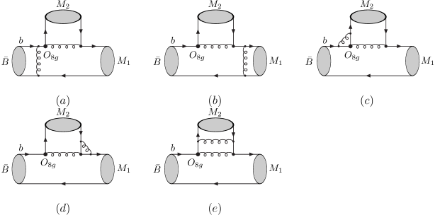
Figure 4: Representative diagrams induced by $b\to Dg^{\ast}g^{\ast}$ transition which are not evaluated. Here we give only the chromo-magnetic dipole operator $Q_{8g}$ contributions. With $\mathcal{O}_{8g}$ replaced by the other operators, the corresponding diagrams for these operators can also be obtained.

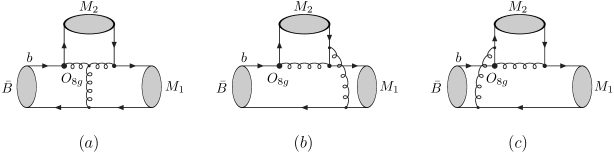
Figure 5: Chromo-magnetic operator $Q_{8g}$ contributions induced by $b\to Dg^{\ast}g^{\ast}$ transition.

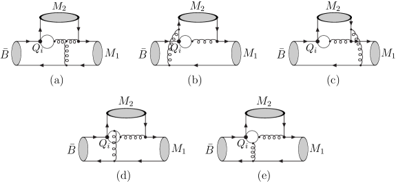
Figure 6: Strong penguin contributions induced by $b\to Dg^{\ast}g^{\ast}$ transition.

As can be seen from Figs. 5 and 6, these penguin diagrams should be the dominant contributions of order $\alpha_{s}^{2}$, since they are not two-loop QCD diagrams and there is no additional $\frac{1}{16\pi^{2}}$ suppression factor compared to the genuine two-loop contributions of order $\alpha_{s}^{2}$. Studies of these contributions could be helpful for understanding the higher order perturbative corrections within the QCDF formalism. In followings, we first discuss these higher order strong penguin contributions to decay modes with two light pseudoscalar mesons in the final states, $B\to M_{1}M_{2}$, and then specialize this general case to the $B\to\pi K,\pi\pi$ decays and investigate the effect of these higher order corrections on the branching ratios and $CP$ asymmetries for these modes.

We start with the calculation of the diagrams in Fig. 5. In this case, the weak decay is induced by the chromo-magnetic dipole operator $O_{8g}$. The calculation is straightforward with the result given by

$${\cal A}_{Q_{8g}} = -i\,\frac{\alpha_{s}^{2}\,f_{B}\,f_{M_{1}}\,f_{M_{2}}}{N_{c}^{3}}\,\lambda_{t}^{(\prime)}\,\int_{0}^{1}\!d{\xi}\,\frac{\Phi_{1}^{B}(\xi)}{\xi}\,$$ (31)

$$\mbox{\,}\times\int_{0}^{1}\!dudv\,\left\{\Phi_{M_{2}}(u)\,\Phi_{M_{1}}(v)\,\left[\frac{1}{6\,\left(1-u\right)\,\left(1-v\right)}+\frac{3\,\left(3-v\right)}{2\,\left(1-u\right)\,\left(1-v\right)\,v}\,\right]\,\right.$$

$$\mbox{\,}+\left.r_{\chi}^{M_{1}}\,\Phi_{M_{2}}(u)\,\Phi_{p}^{M_{1}}(v)\,\left[\frac{2-u}{6\,\left(1-u\right)\,u\,\left(1-v\right)}+\frac{3\,\left(3-u-v+u\,v\right)}{2\,\left(1-u\right)^{2}\,\left(1-v\right)\,v}\,\right]\,\right.$$

$$\mbox{\,}+\left.r_{\chi}^{M_{2}}\,\Phi_{p}^{M_{2}}(u)\,\Phi_{M_{1}}(v)\,\left[\frac{1+u}{6\,\left(1-u\right)\,\left(1-v\right)}+\frac{3\,\left(3-u-v-u\,v\right)}{2\,\left(1-u\right)\,\left(1-v\right)\,v}\,\right]\,\right.$$

$$\mbox{\,}+\left.r_{\chi}^{M_{1}}\,r_{\chi}^{M_{2}}\,\Phi_{p}^{M_{2}}(u)\,\Phi_{p}^{M_{1}}(v)\,\left[\frac{1}{6\,\left(1-u\right)\,\left(1-v\right)}+\frac{3\,\left(3-v\right)}{2\,\left(1-u\right)\,\left(1-v\right)\,v}\,\right]\,\right\},$$

where $\lambda_{t}=V_{tb}V_{ts}^{\ast}$ (for $b\to s$ transition) and $\lambda_{t}^{\prime}=V_{tb}V_{td}^{\ast}$ (for $b\to d$ transition) are products of the CKM matrix elements. As always, $\Phi_{M}$ and $\Phi_{p}^{M}$ denote the leading-twist and twist-3 LCDAs of the pseudoscalar meson $M$ in the final state, respectively.

In calculation of the Feynman diagrams of Fig. 6, we follow the method proposed by Greub and Liniger [45]. First, we calculate the fermion loops in these individual diagrams, and then insert these building blocks into the entire diagrams to obtain the total contributions. In evaluating the internal quark loop diagrams, we shall adopt the naive dimensional regularization (NDR) scheme and the modified minimal subtraction ($\overline{\rm MS}$) scheme. In addition, we shall adopt the ad hoc Feynman gauge throughout this paper. Similar to the calculation of the penguin contractions in Appendix A, we should consider the two distinct contractions in the weak interaction vertex of these penguin diagrams.

As can be seen from Fig. 6, the first three diagrams have the same building block $I_{\mu}^{a}(k)$ (corresponding to the contraction of operators $Q_{1,3}$) or $\tilde{I}_{\mu}^{a}(k)$ (associated with the contractions of the operators $Q_{4,6}$). These building blocks are shown in Fig. 7 and given by

$$I_{\mu}^{a}(k) = \frac{g_{s}}{4\,\pi^{2}}\,\Gamma(\frac{\epsilon}{2})\,(2-\epsilon)\,(4\pi\mu^{2})^{\frac{\epsilon}{2}}\,(k_{\mu}\,\hbox to0.0pt{\hskip 0.56917pt/\hss}{k}-k^{2}\gamma_{\mu})\,(1-\gamma_{5})\,T^{a}\,$$ (32)

$$\mbox{\,}\times\int_{0}^{1}\!dx\,\frac{x\,(1-x)}{\left[m_{q}^{2}-x(1-x)\,k^{2}-i\,\delta\,\right]^{\frac{\epsilon}{2}}}\,,$$

$$\tilde{I}_{\mu}^{a}(k) = \frac{g_{s}}{2\,\pi^{2}}\,\Gamma(\frac{\epsilon}{2})\,(4\pi\mu^{2})^{\frac{\epsilon}{2}}\,(k_{\mu}\,\hbox to0.0pt{\hskip 0.56917pt/\hss}{k}-k^{2}\gamma_{\mu})\,(1-\gamma_{5})\,T^{a}\,$$ (33)

$$\mbox{\,}\times\int_{0}^{1}\!dx\,\frac{x\,(1-x)}{\left[m_{q}^{2}-x(1-x)\,k^{2}-i\,\delta\,\right]^{\frac{\epsilon}{2}}}\,,$$

where $k$ and $T^{a}$ is the momentum and the color generator of the off-shell gluon, $g_{s}$ is the strong coupling constant, and $m_{q}$ the pole mass of the quark propagating in the quark loops. The free indices $\mu$ and $a$ should be contracted with the gluon propagator when inserting these building blocks into the entire diagrams. Here we have used the $d$ dimension space-time as $d=4-\epsilon$. After performing the subtraction with the $\overline{\rm MS}$ scheme, we get

$$I_{\mu}^{a}(k) = \frac{g_{s}}{8\,\pi^{2}}\left[-\frac{2}{3}-\frac{4}{3}\,\ln\frac{m_{b}}{\mu}+G(s_{q},1-u)\,\right](k_{\mu}\,\hbox to0.0pt{\hskip 0.56917pt/\hss}{k}-k^{2}\gamma_{\mu})\,(1-\gamma_{5})\,T^{a}\,,$$ (34)

$$\tilde{I}_{\mu}^{a}(k) = \frac{g_{s}}{8\,\pi^{2}}\left[-\frac{4}{3}\,\ln\frac{m_{b}}{\mu}+G(s_{q},1-u)\,\right](k_{\mu}\,\hbox to0.0pt{\hskip 0.56917pt/\hss}{k}-k^{2}\gamma_{\mu})\,(1-\gamma_{5})\,T^{a}\,,$$ (35)

with the function $G(s,u)$ defined by Eq. (76).

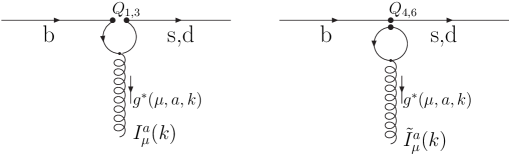
Figure 7: Building blocks $I_{\mu}^{a}(k)$ (associated with the contraction of the operators $Q_{1,3}$) and $\tilde{I}_{\mu}^{a}(k)$ (associated with the contraction of the operators $Q_{4,6}$) for Figs. 6(a)–6(c).

The sum of the fermion loops in the last two diagrams in Fig. 6 are denoted by the building block $J_{\mu\nu}^{ab}(k,p)$ (corresponding to the contraction of operators $Q_{1,3}$) or $\tilde{J}_{\mu\nu}^{ab}(k,p)$ (corresponding to the contraction of operators $Q_{4,6}$), as depicted by Fig. 8. Using the decomposition advocated by [44, 45], these building blocks can be expressed as

$$J^{ab}_{\mu\nu}(k,p) = T^{+}_{\mu\,\nu}(k,p)\,\Big{\{}T^{a},T^{b}\Big{\}}+T^{-}_{\mu\,\nu}(k,p)\Big{[}T^{a},T^{b}\Big{]}\,,$$ (36)

$$\tilde{J}^{ab}_{\mu\nu}(k,p) = \tilde{T}^{+}_{\mu\,\nu}(k,p)\,\Big{\{}T^{a},T^{b}\Big{\}}+\tilde{T}^{-}_{\mu\,\nu}(k,p)\Big{[}T^{a},T^{b}\Big{]}\,,$$ (37)

where the first part is symmetric, while the second one is antisymmetric with respect to the color structures of the two gluons. Here $k(p)$, $a(b)$, and $\mu(\nu)$ are the momentum, color, and polarization of the off-shell gluons. Below, we refer to the gluon with indices $(\nu,b,p)$ as the one connecting with the spectator quark from the $B$ meson.

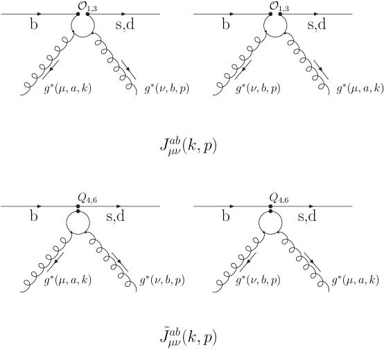
Figure 8: Building blocks $J_{\mu\nu}^{ab}(k,p)$ (associated with operators $Q_{1,3}$) and $\tilde{J}_{\mu\nu}^{ab}(k,p)$ (associated with operators $Q_{4,6}$) for Figs. 6(d) and 6(e).

In the NDR scheme, after integrating over the (shifted) loop momentum, we can present the quantities $T^{\pm}_{\mu\,\nu}(k,p)$ and $\tilde{T}^{\pm}_{\mu\,\nu}(k,p)$ as [44, 45]

$$T^{+}_{\mu\,\nu}(k,p) = \frac{\alpha_{s}}{4\,\pi}\,\biggl{[}E(\mu,\nu,k)\,\Delta i_{5}\,+E(\mu,\nu,p)\,\Delta i_{6}\,\biggr{.}$$ (38)

$$\mbox{\,}\biggl{.}-E(\mu,k,p)\,\frac{k_{\nu}}{k\cdot p}\,\Delta i_{23}-E(\mu,k,p)\,\frac{p_{\nu}}{k\cdot p}\,\Delta i_{24}\biggr{.}$$

$$\mbox{\,}\biggl{.}-E(\nu,k,p)\,\frac{k_{\mu}}{k\cdot p}\,\Delta i_{25}-E(\nu,k,p)\,\frac{p_{\mu}}{k\cdot p}\,\Delta i_{26}\,\biggr{]}\,(1-\gamma_{5})\,,$$

$$T^{-}_{\mu\,\nu}(k,p) = \frac{\alpha_{s}}{4\,\pi}\,\biggl{[}\hbox to0.0pt{\hskip 0.56917pt/\hss}{k}\,g_{\mu\nu}\,\Delta i_{2}+\hbox to0.0pt{\hskip 0.56917pt/\hss}{p}\,g_{\mu\nu}\,\Delta i_{3}\biggr{.}$$ (39)

$$\mbox{\,}\biggl{.}+\gamma_{\mu}\,k_{\nu}\,\Delta i_{8}+\gamma_{\mu}\,p_{\nu}\,\Delta i_{9}+\gamma_{\nu}\,k_{\mu}\,\Delta i_{11}+\gamma_{\nu}\,p_{\mu}\,\Delta i_{12}\biggr{.}$$

$$\mbox{\,}\biggl{.}+\hbox to0.0pt{\hskip 0.56917pt/\hss}{k}\,\frac{k_{\mu}k_{\nu}}{k\cdot p}\,\Delta i_{15}+\hbox to0.0pt{\hskip 0.56917pt/\hss}{k}\,\frac{k_{\mu}p_{\nu}}{k\cdot p}\,\Delta i_{16}+\hbox to0.0pt{\hskip 0.56917pt/\hss}{k}\,\frac{p_{\mu}k_{\nu}}{k\cdot p}\,\Delta i_{17}+\hbox to0.0pt{\hskip 0.56917pt/\hss}{k}\,\frac{p_{\mu}p_{\nu}}{k\cdot p}\,\Delta i_{18}\,\biggr{.}$$

$$\mbox{\,}\biggl{.}+\hbox to0.0pt{\hskip 0.56917pt/\hss}{p}\,\frac{k_{\mu}k_{\nu}}{k\cdot p}\,\Delta i_{19}+\hbox to0.0pt{\hskip 0.56917pt/\hss}{p}\,\frac{k_{\mu}p_{\nu}}{k\cdot p}\,\Delta i_{20}+\hbox to0.0pt{\hskip 0.56917pt/\hss}{p}\,\frac{p_{\mu}k_{\nu}}{k\cdot p}\,\Delta i_{21}+\hbox to0.0pt{\hskip 0.56917pt/\hss}{p}\,\frac{p_{\mu}p_{\nu}}{k\cdot p}\,\Delta i_{22}\,\biggr{]}\,(1-\gamma_{5})\,,$$

$$\tilde{T}^{+}_{\mu\,\nu}(k,p) = a\,T^{+}_{\mu\,\nu}(k,p)\,,$$ (40)

$$\tilde{T}^{-}_{\mu\,\nu}(k,p) = T^{-}_{\mu\,\nu}(k,p)\,+\frac{\alpha_{s}}{4\,\pi}\,\biggl{[}\hbox to0.0pt{\hskip 0.56917pt/\hss}{k}\,g_{\mu\nu}\,\frac{4}{3}\,-\hbox to0.0pt{\hskip 0.56917pt/\hss}{p}\,g_{\mu\nu}\,\frac{4}{3}\,-\gamma_{\mu}\,k_{\nu}\,\frac{8}{3}\,-\gamma_{\mu}\,p_{\nu}\,\frac{4}{3}\,\biggr{.}$$ (41)

$$\mbox{\,}\biggl{.}+\gamma_{\nu}\,k_{\mu}\,\frac{4}{3}\,+\gamma_{\nu}\,p_{\mu}\,\frac{8}{3}\,\biggr{]}\,(1-\gamma_{5})\,,$$

where the matrix $E$ in Eq. (38) is defined by

$$E(\mu,\nu,k) = \gamma_{\mu}\gamma_{\nu}\hbox to0.0pt{\hskip 0.56917pt/\hss}{k}\,-\gamma_{\mu}k_{\nu}\,+\gamma_{\nu}k_{\mu}\,-\hbox to0.0pt{\hskip 0.56917pt/\hss}{k}\,g_{\mu\,\nu}\,$$ (42)

$$= -i\,\epsilon_{\mu\nu\alpha\beta}\,k^{\alpha}\gamma^{\beta}\gamma_{5}\,,$$

with the second line obtained in a four dimension context with the Bjorken-Drell conventions. The parameter $a$ in Eq. (40) denotes the chiral structure of the local four-quark operators in the weak interaction vertex with $a=\pm$ corresponding to $(V-A)\otimes(V\mp A)$, respectively. The dimensionally regularized expressions for the $\Delta i$ functions are collected in Appendix B.

Equipped with the explicit form for these building blocks, we can now evaluate all the Feynman diagrams in Fig. 6. After direct calculations, the final results with the subscript denoting the contraction of the corresponding operator in the weak interaction vertex are

$${\cal A}_{Q_{1}} = i\,\frac{\alpha_{s}^{2}\,f_{B}\,f_{M_{1}}\,f_{M_{2}}}{N_{c}^{3}}\,\lambda_{p}^{(\prime)}\,\int_{0}^{1}\!d{\xi}\,\frac{\Phi_{1}^{B}(\xi)}{\xi}\,\,$$ (43)

$$\mbox{\,}\times\int_{0}^{1}\!dudv\,\left[-\frac{2}{3}-\frac{4}{3}\,\ln{\frac{m_{b}}{\mu}}+G(s_{p},1-u)\,\right]\,f_{1}(u,v)\,$$

$$+ i\,\frac{\alpha_{s}^{2}\,f_{B}\,f_{M_{1}}\,f_{M_{2}}}{N_{c}^{3}}\,\lambda_{p}^{(\prime)}\,\int_{0}^{1}\!d{\xi}\,\frac{\Phi_{1}^{B}(\xi)}{\xi}\,\int_{0}^{1}\!dudv\,f_{2}(u,v,m_{p})\,,$$

$${\cal A}_{Q_{3}} = -i\,\frac{\alpha_{s}^{2}\,f_{B}\,f_{M_{1}}\,f_{M_{2}}}{N_{c}^{3}}\,\lambda_{t}^{(\prime)}\,\int_{0}^{1}\!d{\xi}\,\frac{\Phi_{1}^{B}(\xi)}{\xi}\,$$ (44)

$$\mbox{\,}\times\int_{0}^{1}\!dudv\,\left[-\frac{4}{3}-\frac{8}{3}\,\ln{\frac{m_{b}}{\mu}}+G(0,1-u)+G(1,1-u)\,\right]\,f_{1}(u,v)\,$$

$$- i\,\frac{\alpha_{s}^{2}\,f_{B}\,f_{M_{1}}\,f_{M_{2}}}{N_{c}^{3}}\,\lambda_{t}^{(\prime)}\,\int_{0}^{1}\!d{\xi}\,\frac{\Phi_{1}^{B}(\xi)}{\xi}\,\int_{0}^{1}\!dudv\,\left[f_{2}(u,v,0)+f_{2}(u,v,m_{b})\,\right]\,,$$

$${\cal A}_{Q_{4}} = -i\,\frac{\alpha_{s}^{2}\,f_{B}\,f_{M_{1}}\,f_{M_{2}}}{N_{c}^{3}}\,\lambda_{t}^{(\prime)}\,\int_{0}^{1}\!d{\xi}\,\frac{\Phi_{1}^{B}(\xi)}{\xi}\,\int_{0}^{1}\!dudv\,$$ (45)

$$\mbox{\,}\times\left[-\frac{4\,n_{f}}{3}\,\ln\frac{m_{b}}{\mu}+(n_{f}-2)\,G(0,1-u)\,+G(s_{c},1-u)\,+G(1,1-u)\,\right]\,f_{1}(u,v)\,$$

$$- i\,\frac{\alpha_{s}^{2}\,f_{B}\,f_{M_{1}}\,f_{M_{2}}}{N_{c}^{3}}\,\lambda_{t}^{(\prime)}\,\int_{0}^{1}\!d{\xi}\,\frac{\Phi_{1}^{B}(\xi)}{\xi}\,\int_{0}^{1}\!dudv\,$$

$$\mbox{\,}\times\left[(n_{f}-2)\,f_{3}(u,v,0)\,+f_{3}(u,v,m_{c})+f_{3}(u,v,m_{b})\,\right]\,,$$

$${\cal A}_{Q_{6}} = -i\,\frac{\alpha_{s}^{2}\,f_{B}\,f_{M_{1}}\,f_{M_{2}}}{N_{c}^{3}}\,\lambda_{t}^{(\prime)}\,\int_{0}^{1}\!d{\xi}\,\frac{\Phi_{1}^{B}(\xi)}{\xi}\,\int_{0}^{1}\!dudv\,$$ (46)

$$\mbox{\,}\times\left[-\frac{4\,n_{f}}{3}\,\ln\frac{m_{b}}{\mu}+(n_{f}-2)\,G(0,1-u)\,+G(s_{c},1-u)+G(1,1-u)\right]\,f_{1}(u,v)\,$$

$$- i\,\frac{\alpha_{s}^{2}\,f_{B}\,f_{M_{1}}\,f_{M_{2}}}{N_{c}^{3}}\,\lambda_{t}^{(\prime)}\,\int_{0}^{1}\!d{\xi}\,\frac{\Phi_{1}^{B}(\xi)}{\xi}\,\int_{0}^{1}\!dudv\,$$

$$\mbox{\,}\times\left[(n_{f}-2)\,f_{4}(u,v,0)\,+f_{4}(u,v,m_{c})+f_{4}(u,v,m_{b})\,\right]\,,$$

with

$$f_{1}(u,v) = \Phi_{M_{2}}(u)\,\Phi_{M_{1}}(v)\,\left[\frac{1}{12\,\left(1-u\right)\,\left(1-v\right)}+\frac{3\,\left(3-2\,u-v\right)}{4\,\left(1-u\right)\,\left(1-v\right)\,v}\,\right]\,$$ (47)

$$+ r_{\chi}^{M_{1}}\,\Phi_{M_{2}}(u)\,\Phi_{p}^{M_{1}}(v)\,\left[\frac{3\,\left(3-v\right)}{4\,\left(1-u\right)\,\left(1-v\right)\,v}+\frac{2-u}{12\,\left(1-u\right)\,u\,\left(1-v\right)}\,\right]\,$$

$$- r_{\chi}^{M_{1}}r_{\chi}^{M_{2}}\,\Phi_{p}^{M_{2}}(u)\,\Phi_{p}^{M_{1}}(v)\,\left[\frac{1}{12\,\left(1-u\right)\,\left(1-v\right)}-\frac{3\,\left(3-2\,u-v+2\,u\,v\right)}{4\,\left(1-u\right)\,\left(1-v\right)\,v}\,\right]\,$$

$$+ r_{\chi}^{M_{2}}\,\Phi_{p}^{M_{2}}(u)\,\Phi_{M_{1}}(v)\,\left[\frac{1}{12\,\left(1-v\right)}+\frac{3\,\left(3-v\right)}{4\,\left(1-v\right)\,v}\right]\,,$$

$$f_{2}(u,v,m_{q}) = \Phi_{M_{2}}(u)\,\Phi_{M_{1}}(v)\,\left[\frac{3\,\Delta i_{2}}{8\,\left(1-u\right)\,\left(1-v\right)}+\frac{3\,\Delta i_{3}}{8\,\left(1-u\right)\,v}+\frac{7\,\Delta i_{6}}{24\,\left(1-u\right)\,v}\,\,\right.\,$$ (48)

$$\left.\,+\frac{3\,\Delta i_{8}}{8\,\left(1-v\right)\,v}+\frac{7\,\Delta i_{23}}{24\,\left(1-v\right)\,v}+\frac{7\,\left(1-u+v\right)\,\Delta i_{5}}{24\,\left(1-u\right)\,\left(1-v\right)\,v}\,\right]\,$$

$$- r_{\chi}^{M_{1}}\,\Phi_{M_{2}}(u)\,\Phi_{p}^{M_{1}}(v)\,\left[\frac{3}{8\,\left(1-u\right)\,v}\,\left(\Delta i_{3}+\Delta i_{21}\right)+\frac{3\,\Delta i_{12}}{4\,\left(1-u\right)\,v}\,\right.\,$$

$$\left.+\frac{7}{24\,\left(1-u\right)\,v}\,\left(\Delta i_{6}+\Delta i_{26}\right)+\frac{7\,\Delta i_{5}}{12\,\left(1-u\right)\,\left(1-v\right)}\,\right.\,$$

$$\left.+\frac{3}{8\,\left(1-u\right)\,\left(1-v\right)}\,\left(\Delta i_{2}-\Delta i_{8}+\Delta i_{17}\right)\,\right]\,$$

$$- r_{\chi}^{M_{2}}\,\Phi_{p}^{M_{2}}(u)\,\Phi_{M_{1}}(v)\,\left[\frac{3\,\Delta i_{2}}{8\,\left(1-v\right)\,v}+\frac{7\,\Delta i_{23}}{24\,\left(1-v\right)\,v}+\frac{7\,\Delta i_{5}}{12\,\left(1-v\right)\,v}\,\right.\,$$

$$\left.-\frac{3\,\Delta i_{8}}{8\,\left(1-v\right)}\,\right]\,$$

$$+ r_{\chi}^{M_{1}}r_{\chi}^{M_{2}}\,\Phi_{p}^{M_{2}}(u)\,\Phi_{p}^{M_{1}}(v)\,\left[\frac{7\,\Delta i_{5}}{12\,\left(1-v\right)}-\frac{3\,\Delta i_{12}}{8\,v}-\frac{7\,u\,\Delta i_{23}}{12\,\left(1-u\right)\,\left(1-v\right)}\,\right.\,$$

$$\left.+\frac{3\,u}{8\,\left(1-u\right)\,v}\,\left(\Delta i_{3}+\Delta i_{21}\right)\,+\frac{7}{24\,\left(1-u\right)\,v}\,\left(\Delta i_{6}+\Delta i_{26}\right)\,\right.\,$$

$$\left.+\frac{3}{8}\,\left(\frac{1}{\left(1-u\right)\,\left(1-v\right)}+\frac{1}{v}\right)\,\left(\Delta i_{2}+\Delta i_{8}+\Delta i_{17}\right)\,\right]\,,$$

$$f_{3,(4)}(u,v,m_{q}) = \Phi_{M_{2}}(u)\,\Phi_{M_{1}}(v)\,\left[-\frac{\left(3-2\,u-2\,v\right)}{2\,\left(1-u\right)\,\left(1-v\right)\,v}+\frac{3\,\Delta i_{2}}{8\,\left(1-u\right)\,\left(1-v\right)}+\frac{3\,\Delta i_{3}}{8\,\left(1-u\right)\,v}\,\right.\,$$ (49)

$$\left.\pm\frac{7\,\left(1-u+v\right)\,\Delta i_{5}}{24\,\left(1-u\right)\,\left(1-v\right)\,v}\,\pm\frac{7\,\Delta i_{6}}{24\,\left(1-u\right)\,v}\,+\frac{3\,\Delta i_{8}}{8\,\left(1-v\right)\,v}\pm\frac{7\,\Delta i_{23}}{24\,\left(1-v\right)\,v}\,\right]\,$$

$$- r_{\chi}^{M_{1}}\,\Phi_{M_{2}}(u)\,\Phi_{p}^{M_{1}}(v)\,\left[\frac{3}{2\,\left(1-u\right)\,\left(1-v\right)\,v}+\frac{3}{8\,\left(1-u\right)\,v}\,\left(\Delta i_{3}+\Delta i_{21}\right)\,\right.\,$$

$$\left.\pm\frac{7}{24\,\left(1-u\right)\,v}\,\left(\Delta i_{6}+\Delta i_{26}\right)+\frac{3\,\Delta i_{12}}{4\,\left(1-u\right)\,v}\pm\frac{7\,\Delta i_{5}}{12\,\left(1-u\right)\,\left(1-v\right)}\,\right.\,$$

$$\left.+\frac{3}{8\,\left(1-u\right)\,\left(1-v\right)}\,\left(\Delta i_{2}-\Delta i_{8}+\Delta i_{17}\right)\,\right]\,$$

$$- r_{\chi}^{M_{2}}\,\Phi_{p}^{M_{2}}(u)\,\Phi_{M_{1}}(v)\,\left[\frac{3}{2\,\left(1-v\right)\,v}+\frac{3\,\Delta i_{2}}{8\,\left(1-v\right)\,v}\pm\frac{7\,\Delta i_{23}}{24\,\left(1-v\right)\,v}\,\right.\,$$

$$\left.\pm\frac{7\,\Delta i_{5}}{12\,\left(1-v\right)\,v}\,-\frac{3\,\Delta i_{8}}{8\,\left(1-v\right)}\,\right]\,$$

$$+ r_{\chi}^{M_{1}}r_{\chi}^{M_{2}}\,\Phi_{p}^{M_{2}}(u)\,\Phi_{p}^{M_{1}}(v)\,\left[-\frac{3-2\,u-2\,v+2\,u\,v}{2\,\left(1-u\right)\,\left(1-v\right)\,v}\pm\frac{7\,\Delta i_{5}}{12\,\left(1-v\right)}-\frac{3\,\Delta i_{12}}{8\,v}\,\right.\,$$

$$\left.\mp\frac{7\,u\,\Delta i_{23}}{12\,\left(1-u\right)\,\left(1-v\right)}+\frac{3\,u}{8\,\left(1-u\right)\,v}\,\left(\Delta i_{3}+\Delta i_{21}\right)\,\right.\,$$

$$\left.\,\pm\frac{7}{24\,\left(1-u\right)\,v}\,\left(\Delta i_{6}+\Delta i_{26}\right)\,\right.\,$$

$$\left.+\frac{3}{8}\,\left(\frac{1}{\left(1-u\right)\,\left(1-v\right)}+\frac{1}{v}\right)\,\left(\Delta i_{2}+\Delta i_{8}+\Delta i_{17}\right)\,\right]\,,$$

where the argument $m_{q}$ is the quark mass propagating in the fermion loops. At this stage, the $\Delta_{i}$ functions are the ones that have been performed the Feynman parameter integrals, whose explicit forms can be found in Appendix B.

With the individual operator contributions given above, the total contributions of these higher order $b\to Dg^{\ast}g^{\ast}$ strong penguin diagrams to the decay amplitudes of $B\to M_{1}M_{1}$ modes can be written as

$${\cal A}_{b\to Dg^{\ast}g^{\ast}}=\frac{G_{F}}{\sqrt{2}}\,\left[{C_{8g}^{\rm eff}\,\cal A}_{Q_{8g}}+C_{1}\,{\cal A}_{Q_{1}}+C_{3}\,{\cal A}_{Q_{3}}+C_{4}\,{\cal A}_{Q_{4}}+C_{6}\,{\cal A}_{Q_{6}}\,\right]\,.$$ (50)

In order to specialize these general results to $B\to\pi K,\pi\pi$ decays, we just need to replace $M_{1}$ and $M_{2}$ with the corresponding mesons. Explicitly, the $b\to Dg^{\ast}g^{\ast}$ strong penguin contributions to the decay amplitudes of the four $B\to\pi K$ and the three $B\to\pi\pi$ decay channels are

$${\cal A}^{\prime}(B^{-}\to\pi^{-}\overline{K}^{0}) = {\cal A}^{\prime}(\overline{B}^{0}\to\pi^{+}K^{-})={\cal A}_{b\to sg^{\ast}g^{\ast}}\,(M_{1}\to\pi,M_{2}\to K)\,,$$

$$\sqrt{2}\,{\cal A}^{\prime}(B^{-}\to\pi^{0}K^{-}) = -\sqrt{2}\,{\cal A}^{\prime}(\overline{B}^{0}\to\pi^{0}\overline{K}^{0})={\cal A}_{b\to sg^{\ast}g^{\ast}}\,(M_{1}\to\pi,M_{2}\to K)\,,$$ (51)

$${\cal A}^{\prime}(\overline{B}^{0}\to\pi^{+}\pi^{-}) = {\cal A}^{\prime}(\overline{B}^{0}\to\pi^{0}\pi^{0})={\cal A}_{b\to dg^{\ast}g^{\ast}}\,(M_{1}\to\pi,M_{2}\to\pi)\,,$$

$${\cal A}^{\prime}(B^{-}\to\pi^{-}\pi^{0}) = 0\,,$$ (52)

where the superscript ‘$\prime$’ is indicated there to be distinguished from the next-to-leading order results given by Eqs. (2.2) and (19). The total decay amplitudes are then the sum of these two pieces.

With the total decay amplitudes, the branching ratio for $B\to M_{1}M_{2}$ decays reads

$${\cal B}(B\to M_{1}M_{2})=\frac{\tau_{B}\,p_{c}}{8\,\pi\,m_{B}^{2}}\,\left|{\cal A}(B\to M_{1}M_{2})+{\cal A}^{{}^{\prime}}(B\to M_{1}M_{2})\,\right|^{2}\,\cdot\,S\,,$$ (53)

where $\tau_{B}$ is the lifetime of the $B$ meson, $S=1/2$ if $M_{1}$ and $M_{2}$ are identical, and $S=1$ otherwise. $p_{c}$ is the magnitude of the momentum of the final-state particle $M_{1,2}$ in the $B$ meson rest frame and given by

$$p_{c}=\frac{1}{2m_{B}}\sqrt{\left[m_{B}^{2}-(m_{M_{1}}+m_{M_{2}})^{2}\,\right]\,\left[m_{B}^{2}-(m_{M_{1}}-m_{M_{2}})^{2}\,\right]}\,.$$ (54)

As for the direct $CP$ asymmetries, we use the definition of the difference of the $\bar{B}$-meson minus $B$-meson decay rates divided by their sum. With the branching ratios of the $CP$-conjugated modes denoted by ${\cal B}(\bar{B}\to\bar{f})$, the $CP$-averaged branching ratios and the direct $CP$ asymmetries for $B\to f$ decays can be expressed respectively as

$$\bar{\cal B} = \frac{1}{2}\,\left[{\cal B}(\bar{B}\to\bar{f})+{\cal B}(B\to f)\,\right]\,,$$ (55)

$${\cal A}_{CP} = \frac{{\cal B}(\bar{B}\to\bar{f})-{\cal B}(B\to f)}{{\cal B}(\bar{B}\to\bar{f})+{\cal B}(B\to f)}\,.$$ (56)

3 Numerical calculation and Discussions

3.1 Input parameters

The theoretical predictions with the QCDF approach depend on many input parameters such as the CKM matrix elements, Wilson coefficients, hadronic parameters, and so on. We present all the relevant input parameters as follows.

-Wilson coefficients. The Wilson coefficients $C_{i}(\mu)$ in the effective weak Hamiltonian have been reliably evaluated to the next-to-leading logarithmic order. To proceed, we use the following numerical values at $\mu=m_{b}$ scale, which have been obtained in the NDR scheme [49, 58]

$$\begin{array}[]{llll}C_{1}=1.082,&C_{2}=-0.185,&C_{3}=0.014,&C_{4}=-0.035,\\ C_{5}=0.009,&C_{6}=-0.041,&C_{7}/\alpha=-0.011,&C_{8}/\alpha=0.059,\\ C_{9}/\alpha=-1.241,&C_{10}/\alpha=0.218,&C_{7\gamma}^{\rm eff}=-0.299,&C_{8g}^{\rm eff}=-0.143.\end{array}$$ (57)

-The CKM matrix elements. The widely used parametrization of the CKM matrix elements in analyzing $B$-meson decays is the Wolfenstein parametrization, which emphasizes the hierarchies among its elements and is expanded as a power series in the parameter $\lambda=|V_{us}|$ [59],

$$V_{\rm CKM}=\left(\begin{array}[]{ccc}1-\frac{\lambda^{2}}{2}&\lambda&A\lambda^{3}(\rho-i\eta)\\ -\lambda&1-\frac{\lambda^{2}}{2}&A\lambda^{2}\\ A\lambda^{3}(1-\rho-i\eta)&-A\lambda^{2}&1\\ \end{array}\right)\,+{\cal O}(\lambda^{4})\,.$$ (58)

The values of the four Wolfenstein parameters ($A$, $\lambda$, $\rho$, and $\eta$) could be determined from the best knowledge of the experimental and theoretical inputs. In this paper, we take

$$A=0.8533,\qquad\lambda=0.2200,\qquad\bar{\rho}=0.20,\qquad\bar{\eta}=0.33,$$ (59)

as our default input values [60]. The parameters $\bar{\rho}$ and $\bar{\eta}$ are defined by $\bar{\rho}=\rho\,(1-\frac{\lambda^{2}}{2})\,,\bar{\eta}=\eta\,(1-\frac{\lambda^{2}}{2})$.

-Masses and lifetimes. For the quark mass, there are two different classes appearing in the QCDF approach. One type is the pole quark mass which appears in the evaluation of the penguin loop corrections, and is denoted by $m_{q}$ with $q=u,d,s,c,b$. In this paper, we take

$$m_{u}=m_{d}=m_{s}=0,\qquad m_{c}=1.47\,{\rm GeV},\qquad m_{b}=4.80\,{\rm GeV},$$ (60)

as our default input values.

The other one is the current quark mass which appears in the equations of motion and is used to calculate the matrix elements of the penguin operators as well as the chiral enhancement factors $r_{\chi}^{M}$. This kind of quark mass is scale dependent. To get the corresponding value at the given scale, we should use the renormalization group equation to run them, which can be found, for example, in [49]. Following Ref. [25], we hold $(\overline{m}_{u}+\overline{m}_{d})/\overline{m}_{s}$ fixed and use $\overline{m}_{s}$ as an input parameters. Explicitly, we take

$$\overline{m}_{u}(2\,{\rm GeV}) = \overline{m}_{d}(2\,{\rm GeV})=0.0413\,\overline{m}_{s}(2\,{\rm GeV})\,,$$

$$\overline{m}_{s}(2\,{\rm GeV}) = 90\,{\rm MeV}\,,\qquad\overline{m}_{b}(m_{b})=4.40\,{\rm GeV}\,.$$ (61)

where the difference between the $u$ and $d$ quark is not distinguished.

For meson masses and the lifetimes of the $B$ meson, we adopt the center values given by [60]

$\tau_{B_{u}}=1.671$ ps ,	$\tau_{B_{d}}=1.536$ ps ,	$m_{B_{u}}=5.2794$ GeV ,	$m_{B_{d}}=5.2790$ GeV ,
$m_{K^{\pm}}=493.7$ MeV ,	$m_{K^{0}}=497.6$ MeV ,	$m_{\pi^{\pm}}=139.6$ MeV ,	$m_{\pi^{0}}=135.0$ MeV .

-Light-cone distribution amplitudes of mesons. Since the QCDF approach is based on the heavy quark assumption, to a very good approximation, we can use the asymptotic form of the LCDAs for light mesons [53, 56, 61]

$$\Phi_{M}(x)=6\,x(1-x),\qquad\Phi_{p}^{M}(x)=1.$$ (62)

With respect to the endpoint divergence associated with the momentum fraction integral over the LCDAs appearing in this paper, in analogy to the treatment in Refs. [21, 62], we regulate the integral with an ad-hoc cut-off

$$\int_{0}^{1}\!dv\,\frac{\Phi_{p}^{M}(v)}{1-v}\, \to \int_{0}^{1-\Lambda_{h}/m_{B}}\!dv\,\frac{\Phi_{p}^{M}(v)}{1-v}=\ln\frac{m_{B}}{\Lambda_{h}},$$ (63)

with $\Lambda_{h}=500\,{\rm MeV}$, and do not distinguish whether this divergence comes from the hard spectator rescattering or from the annihilation contributions. The possible complex phase associated with this integral has also been neglected.

As for the $B$ meson wave functions, within our approximation, we need only consider the first inverse moment of the LCDA $\Phi_{1}^{B}(\xi)$ defined by [21]

$$\int_{0}^{1}\frac{d\xi}{\xi}\,\Phi_{1}^{B}(\xi)\equiv\frac{m_{B}}{\lambda_{B}}\,,$$ (64)

where the hadronic parameter $\lambda_{B}$ has been introduced to parameterize this integral. This parameter has been evaluated using different methods [63, 64] recently. In this paper, we take $\lambda_{B}=460\,{\rm MeV}$ as our default input value [63].

-Decay constants and transition form factors. The decay constant and the form factors are nonperturbative parameters and can be determined from experiments and/or theoretical estimations. For the decay constants, we take

$$f_{B}=200\,{\rm MeV}\,\cite[cite]{[\@@bibref{}{bbns3}{}{}]},\qquad f_{K}=160\,{\rm MeV}\,,\qquad f_{\pi}=131\,{\rm MeV}.$$ (65)

For the form factors involving the $B\to K$ and $B\to\pi$ transitions, we take

$$F_{0}^{B\to\pi}(0)=0.258\,,\qquad F_{0}^{B\to K}(0)=0.331\,,$$ (66)

as the default values at the maximum recoil. In addition, we use the formula

$$F_{0}^{B\to M}(q^{2})=\frac{r_{2}^{M}}{1-q^{2}/m_{fit}^{2}(M)}\,,$$ (67)

to parameterize the dependence of the form factor on the momentum-transfer $q^{2}$, with the fit parameters given by

$$r_{2}^{\pi}=0.258\,,\qquad m_{fit}^{2}(\pi)=33.81\,,\qquad r_{2}^{K}=0.330\,,\qquad m_{fit}^{2}(K)=37.46\,.$$ (68)

All of these values are taken from the latest QCD sum rule analysis [65].

3.2 Numerical results and discussions

With the theoretical expressions and the input parameters given above, we can now evaluate the branching ratios and the direct $CP$ asymmetries for $B\to\pi K$ and $B\to\pi\pi$ decays. For each quantity, we first give the predictions at the next-to-leading order in $\alpha_{s}$, and then take into account the $b\to Dg^{\ast}g^{\ast}$ strong penguin corrections, which are of order $\alpha_{s}^{2}$. The combining contributions of the two pieces, denoted by ${\cal O}(\alpha_{s}+\alpha_{s}^{2})$, is then given in the last. For comparison, the NF results are also presented. All the averaged experimental data are taken from HFAG [28].

3.2.1 The $CP$-averaged branching ratios for $B\to\pi K,\pi\pi$ decays

In the SM, the four $B\to\pi K$ decays are dominated by the $b\to s$ strong penguin diagrams, with additional subdominant contributions from the tree and electro-weak penguin diagrams. The three $B\to\pi\pi$ decays, however, are tree-dominated modes. It is therefore expected that these higher order strong penguin diagrams considered in this paper should contribute effectively to $B\to\pi K$ modes, while have only a minor impact on $B\to\pi\pi$ ones. Numerical results of the $CP$-averaged branching ratios for these modes are collected in Table 1.

Table 1: The $CP$-averaged branching ratios (in units of $10^{-6}$) for $B\to\pi K,\pi\pi$ decays with the default input parameters. $\bar{\cal B}^{f}$ and $\bar{\cal B}^{f+a}$ denote the results without and with the annihilation contributions, respectively. The NF results, which are of order ${\cal O}(\alpha_{s}^{0})$, are also shown for comparison. $\bar{\rho}=0.20$ and $\bar{\eta}=0.33$

$\bar{\cal B}^{f}$		$\bar{\cal B}^{f+a}$
Decay Mode	NF	${\cal O}(\alpha_{s})$	${\cal O}(\alpha_{s}+\alpha_{s}^{2})$	${\cal O}(\alpha_{s})$	${\cal O}(\alpha_{s}+\alpha_{s}^{2})$	Exp.
$B^{-}\to\pi^{-}\overline{K}^{0}$	$10.07$	$13.28$	$17.31$	$16.04$	$20.44$	$24.1\pm 1.3$
$B^{-}\to\pi^{0}K^{-}$	$5.69$	$7.30$	$9.37$	$8.72$	$10.97$	$12.1\pm 0.8$
$\overline{B}^{0}\to\pi^{+}K^{-}$	$7.71$	$10.25$	$13.61$	$12.46$	$16.15$	$18.2\pm 0.8$
$\overline{B}^{0}\to\pi^{0}\overline{K}^{0}$	$3.38$	$4.63$	$6.26$	$5.70$	$7.50$	$11.5\pm 1.0$
$\overline{B}^{0}\to\pi^{+}\pi^{-}$	$7.41$	$7.69$	$7.99$	$8.32$	$8.63$	$4.5\pm 0.4$
$B^{-}\to\pi^{-}\pi^{0}$	$5.12$	$5.06$	$5.06$	$-$	$-$	$5.5\pm 0.6$
$\overline{B}^{0}\to\pi^{0}\pi^{0}$	$0.15$	$0.16$	$0.19$	$0.17$	$0.21$	$1.45\pm 0.29$

The dependence of these $CP$-averaged branching ratios on the weak phase $\gamma$ is shown by Fig. 9 (without the annihilation contributions) and Fig. 10 (with the annihilation contributions), where the solid and dashed curves correspond to the theoretical predictions with and without the $b\to Dg^{\ast}g^{\ast}$ strong penguin contributions included, respectively. The horizontal solid lines denote the experimental data as given in Table 1, with the thicker one denoting its center value and the thinner ones its error bars. In these and the following figures, the default values of all inputs parameters except for the CKM angle $\gamma$ are used.

Figure 9: The $\gamma$ dependence of the $CP$-averaged branching ratios for $B\to\pi K,\pi\pi$ decays without the annihilation contributions. The solid and dashed curves correspond to the theoretical predictions with and without the $b\to Dg^{\ast}g^{\ast}$ strong penguin contributions included, respectively. The horizontal solid lines denote the experimental data as given in Table 1, with the thicker ones being its center values and the thinner its error bars.

Figure 10: The $\gamma$ dependence of the $CP$-averaged branching ratios for $B\to\pi K,\pi\pi$ decays with the annihilation contributions included. The meaning of the curves and the horizontal solid lines is the same as in Fig. 9.

From these two figures and the numerical results given by Table 1, we can see that:

• For penguin-dominated $B\to\pi K$ decays, due to the enhancement of the penguin amplitudes, the QCDF scheme prefers larger branching ratios than the NF approximation. With our default input parameters, however, predictions for the branching rations are still smaller than the experimental data even after the inclusion of the annihilation contributions, if we consider only contributions up to the next-to-leading order in $\alpha_{s}$. The effects of these higher order $b\to sg^{\ast}g^{\ast}$ strong penguin corrections are very prominent in these penguin-dominated $B\to\pi K$ decays. With our input parameters, we find that these higher order strong penguin contributions can give $\sim 30\%$ enhancement to the corresponding branching ratios, and such an enhancement can improve the consistency between the theoretical predictions and the experimental data significantly. In addition, we find that the effect of the annihilation contributions on the branching ratios, though not negligible, is not so large as claimed by pQCD method [2, 51].

• For tree-dominated $B\to\pi\pi$ decays, the higher order $b\to dg^{\ast}g^{\ast}$ contributions play only a minor role. To a very good approximation, the $B^{\pm}\to\pi^{\pm}\pi^{0}$ decay can be considered as a pure tree process, and it does not receive annihilation contributions either. The theoretical prediction for the corresponding branching ratio agrees with the data quite well. For the other two $B\to\pi\pi$ modes, however, theoretical predictions with QCDF approach are quite inconsistent with the measured ratios, even with the annihilation and the higher order strong penguin contributions included. With our input parameters, we find that the theoretical prediction for $\bar{B}^{0}\to\pi^{0}\pi^{0}$ mode is about an eighth of the experimental data; for $\bar{B}^{0}\to\pi^{+}\pi^{-}$ mode, on the other hand, a value about two times larger than the data is predicted.

• As for the $\gamma$ dependence of the corresponding branching ratios, we can see that the two decay modes, $B^{\pm}\to\pi^{\pm}\pi^{0}$ and $B^{\pm}\to\pi^{\pm}K^{0}$, are almost independent of this angle, since the corresponding decay amplitudes have to a good approximation only a single weak phase. In addition, the discrepancy between the theoretical prediction and the experimental data for $\overline{B}^{0}\to\pi^{+}\pi^{-}$ can be removed if we use a large angle $\gamma\sim 120^{\circ}$. With the annihilation and the higher order strong penguin contributions included, the four $B\to\pi K$ modes, however, prefer a smaller value for this angle around $\gamma\sim 80^{\circ}$, which is quite consistent with the latest direct experimental measurement $\gamma=81^{\circ}\pm 19^{\circ}(stat.)\pm 13^{\circ}(sys.)\pm 11^{\circ}(model)$ [66].

• The theoretical predictions for the branching ratios are very sensitive to the value of the form factor $F_{0}^{B\to\pi}$. For example, the large measured decay rates for the four $B\to\pi K$ decays can be well accommodated with a larger value of the form factor as shown by Beneke and Neubert [25]. On the other hand, the prediction for $\overline{B}^{0}\to\pi^{+}\pi^{-}$ decays can become consistent with the data only when a smaller value is used. The large measured ratio for $\overline{B}^{0}\to\pi^{0}\pi^{0}$, however, remains unresolved with the varying of these parameters. It is a tough theoretical challenge to accommodate the current experimental data in the SM.

Since the uncertainties in the predictions for branching ratios can be largely eliminated by taking ratios between them, we now discuss the variations of the quantities defined by Eqs. (2)–(6) with the higher order $b\to Dg^{\ast}g^{\ast}$ strong penguin contributions included. It is the known $``\pi K"$ puzzle [29, 30] that the SM predictions are inconsistent with current experiment data. The theoretical predictions and the current experimental data for these ratios are collected in Table 2. For the $\gamma$ dependence of these quantities, we display them in Fig. 11, where the curves and the horizontal solid lines have the same interpretations as in Fig. 9.

Table 2: Ratios between the $CP$-averaged branching fractions for $B\to\pi K,\pi\pi$ modes. The values in the parentheses are the ones without the annihilation contributions.

	NF	${\cal O}(\alpha_{s})$	${\cal O}(\alpha_{s}+\alpha_{s}^{2})$	Exp.
$R_{+-}$	$1.272$	$1.119~{}(1.209)$	$1.077~{}(1.163)$	$2.20\pm 0.31$
$R_{00}$	$0.040$	$0.041~{}(0.042)$	$0.048~{}(0.047)$	$0.67\pm 0.14$
$R$	$0.833$	$0.845~{}(0.840)$	$0.860~{}(0.855)$	$0.82\pm 0.06$
$R_{c}$	$1.130$	$1.087~{}(1.100)$	$1.074~{}(1.083)$	$1.00\pm 0.09$
$R_{n}$	$1.140$	$1.092~{}(1.106)$	$1.077~{}(1.087)$	$0.79\pm 0.08$

Figure 11: Ratios of the $CP$-averaged branching fractions defined by Eqs. (2)–(6) as functions of the weak phase $\gamma$. The meaning of the curves and the horizontal solid lines is the same as in Fig. 9.

From Table 2 and Fig. 11, we can find that the two ratios $R_{c}$ and $R_{n}$ are indeed approximately equal within the SM as claimed in Ref. [30], while the experimental data for the two quantities are quite different with the puzzling pattern $R_{n}<1$. On the other hand, the value of the quantity $R$ predicted by the QCDF approach is well consistent with the experimental data. For the other two ratios $R_{+-}$ and $R_{00}$, the discrepancies between the theoretical predictions and the experimental data are quite large. As the $b\to Dg^{\ast}g^{\ast}$ strong penguin contributions to $B\to\pi K,\pi\pi$ decays are similar in nature, and hence eliminated in the ratios between the corresponding branching fractions, the patterns of the these quantities remain unaffected even with these new strong penguin contributions included. From the $\gamma$ dependence of the ratios between the four $B\to\pi K$ decays, a smaller value for this phase is preferred. On the other hand, a larger value for this phase is favored by $B\to\pi\pi$ decays. These inconsistences may be hints for new physics playing in the electroweak penguin sector as suggested by Buras et al. [30].

3.2.2 The direct $CP$ asymmetries for $B\to\pi K,\pi\pi$ decays

Contrary to the NF approximation, the QCDF scheme can predict the strong interaction phases and hence the direct $CP$ asymmetries in the heavy quark limit. The numerical results and the experimental data for this quantity involving the four $\pi K$ and the three $\pi\pi$ final states are collected in Table 3. The $\gamma$ dependence of the direct $CP$ asymmetries is displayed in Fig. 12 (without the annihilation contributions) and Fig. 13 (with the annihilation contributions), in which the curves and the horizontal solid lines also have the same interpretation as in Fig. 9.

Table 3: The direct $CP$ asymmetries (in units of $10^{-2}$) for $B\to\pi K,\pi\pi$ decays with the default input parameters. $A_{CP}^{f}$ and $A_{CP}^{f+a}$ denote the results without and with the annihilation contributions, respectively.

$A_{CP}^{f}$		$A_{CP}^{f+a}$
Decay Mode	${\cal O}(\alpha_{s})$	${\cal O}(\alpha_{s}+\alpha_{s}^{2})$	${\cal O}(\alpha_{s})$	${\cal O}(\alpha_{s}+\alpha_{s}^{2})$	Exp.
$B^{-}\to\pi^{-}\overline{K}^{0}$	$0.73$	$0.52$	$0.65$	$0.46$	$-2.0\pm 3.4$
$B^{-}\to\pi^{0}K^{-}$	$7.59$	$6.94$	$6.56$	$6.07$	$4\pm 4$
$\overline{B}^{0}\to\pi^{+}K^{-}$	$5.31$	$4.83$	$4.39$	$4.08$	$-10.9\pm 1.9$
$\overline{B}^{0}\to\pi^{0}\overline{K}^{0}$	$-3.08$	$-2.84$	$-2.71$	$-2.54$	$-9\pm 14$
$\overline{B}^{0}\to\pi^{+}\pi^{-}$	$-4.73$	$-5.51$	$-4.54$	$-5.27$	$37\pm 10$
$B^{-}\to\pi^{-}\pi^{0}$	$-0.30$	$-0.31$	$-$	$-$	$-2\pm 7$
$\overline{B}^{0}\to\pi^{0}\pi^{0}$	$55.52$	$58.53$	$55.03$	$55.50$	$28\pm 39$

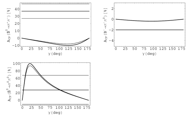
Figure 12: The $\gamma$ dependence of the $CP$ asymmetries without the annihilation contributions. The meaning of the curves and the horizontal solid lines is the same as in Fig. 9.

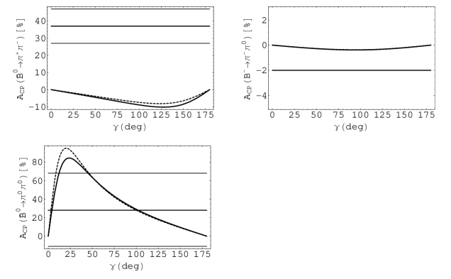
Figure 13: The $\gamma$ dependence of the $CP$ asymmetries with the annihilation contributions included. The meaning of the curves and the horizontal solid lines is the same as in Fig. 9.

From these two figures and the numerical results given in Table 3, we can see that:

• The direct $CP$ asymmetries for $B\to\pi K,\pi\pi$ decays are predicted to be typically small with the QCDF formalism. This could be well understood, since the direct $CP$ asymmetries are proportional to the sines of the strong interaction phases, which are usually suppressed by $\alpha_{s}$ and/or $\Lambda_{QCD}/m_{b}$ within the QCDF formalism. Due to a potentially large relative phase between the QCD penguins and the coefficient $a_{2}$, the $\overline{B}^{0}\to\pi^{0}\pi^{0}$ mode, however, is an exception to this general rule. The direct $CP$ asymmetries for this mode is predicted to be about $55\%$.

• Although the individual Feynman diagram in Fig. 6 carries large strong phase, the combining contributions of these $b\to Dg^{\ast}g^{\ast}$ strong penguin diagrams contain only a relatively small one. Thus, these higher order strong penguin contributions to the direct $CP$ asymmetries are also small.

• The theoretical predictions for $A_{CP}(\overline{B}^{0}\to\pi^{+}\pi^{-})$ and $A_{CP}(\overline{B}^{0}\to\pi^{+}K^{-})$ are quite smaller than the experimental data, particularly with the opposite sign. How to accommodate these discrepancies in the SM is still a challenge.

4 Conclusions

In this paper, we have revisited the $B\to\pi K,\pi\pi$ decays in the framework of QCDF with the $b\to Dg^{\ast}g^{\ast}$ strong penguin contributions included. The main conclusions of this paper are:

1. For penguin-dominated $B\to\pi K$ decays, the higher order strong penguin contributions induced by $b\to sg^{\ast}g^{\ast}$ transitions to the branching ratios are rather large. With our input parameters, we find that these higher order strong penguin contributions can give $\sim 30\%$ enhancement to the corresponding branching ratios, and such an enhancement can improve the consistency between the theoretical predictions and the experimental data significantly .

2. For tree-dominated $B\to\pi\pi$ decays, the higher order $b\to dg^{\ast}g^{\ast}$ contributions to the corresponding branching ratios are quite small.

3. Because of large cancellations among the $b\to Dg^{\ast}g^{\ast}$ strong penguin contributions, only a relatively small strong phase is remained, So that the contributions have small effects on predictions of the direct $CP$ asymmetries.

4. Since corrections of these higher order strong penguin diagrams to the decay amplitudes are similar in nature, and hence cancelled in the ratios between the corresponding branching fractions, the patterns of the quantities $R$, $R_{c}$, $R_{n}$, $R_{+-}$, and $R_{00}$ remain unaffected compared to the next-to-leading order results. So we haven’t found solution to the “$\pi K$” puzzle. Our results indicate that to resolve the puzzle we may have to resort to new physics contributions through the electroweak penguin sector as observed by Buras et al. [30].

5. The theoretical predictions for the branching ratios and the direct $CP$ asymmetries still have large theoretical uncertainties. The dominant errors are induced by the uncertainties of the $F_{0}^{B\to\pi,K}(q^{2})$ form factors, strange quark mass $\overline{m}_{s}(\mu)$, and the CKM angle $\gamma$.

Although the results presented here have still large theoretical uncertainties, the $b\to Dg^{\ast}g^{\ast}$ strong penguin contributions to two-body hadronic $B$-meson decays, particularly to penguin-dominated modes, have been shown to be very important. Further systematic studies on these higher order contributions to charmless $B$ decays are therefore interesting and deserving.

Note added: After this work is finished, we note an interesting study of $\alpha_{s}^{2}$ corrections to $B\to\pi K,\pi\pi$ decays has been carried out by Li, Mishima and Sanda [67] in PQCD formalism. However, the contributions studied here as depicted by the Feynman diagrams in Figs. 5 and 6 are not included in their paper.

Appendix A: Correction functions at next-to-leading order in $\alpha_{s}$

In this appendix, we present the explicit form for the correction functions appearing in the parameters $a_{i}$ and $b_{i}$. Details about the calculation can be found in Refs. [21, 25].

-One-loop vertex corrections. The vertex parameters $V_{i}(M_{2})$ result from the first four diagrams in Fig. 2, given by (with $M_{2}=\pi$, or $K$)

$$V_{i}(M_{2})=\left\{\,\,\begin{array}[]{ll}{\displaystyle\int_{0}^{1}\!du\,\Phi_{M_{2}}(u)\,\Big{[}12\ln\frac{m_{b}}{\mu}-18+g(u)\Big{]}}&\qquad i=\mbox{1--4},9,10,\\[11.38092pt] {\displaystyle\int_{0}^{1}\!du\,\Phi_{M_{2}}(u)\,\Big{[}-12\ln\frac{m_{b}}{\mu}+6-g(1-u)\Big{]}}&\qquad i=5,7,\\[11.38092pt] {\displaystyle\int_{0}^{1}\!du\,\Phi_{p}^{M_{2}}(u)\,[-6\,]}&\qquad i=6,8,\end{array}\right.$$ (69)

with

$$g(u)=3\left[\frac{1-2u}{1-u}\ln u-i\pi\right].$$ (70)

The scheme-dependent constants $-18$, $6$, $-6$ are specific to the NDR scheme for $\gamma_{5}$. $\Phi_{M_{2}}$ and $\Phi_{p}^{M_{2}}$ denote the leading-twist and twist-3 LCDAs of the emitted meson $M_{2}$, respectively.

-Penguin contractions. The QCD and electro-weak penguin parameters $P_{4,6}^{p}$ and $P_{8,10}^{p}$ arise from the diagrams in Figs. 2(e) and 2(f) . Considering the fact that there exist two distinct penguin contractions as shown in Fig. 14, these penguin contributions can be written as

$$P_{4}^{p}(M_{2}) = \frac{C_{F}\alpha_{s}}{4\pi N_{c}}\,\Bigg{\{}C_{1}\!\left[\frac{4}{3}\ln\frac{m_{b}}{\mu}+\frac{2}{3}-G_{M_{2}}(s_{p})\right]\!\Bigg{.}$$ (71)

$$\mbox{}+\Bigg{.}C_{3}\!\left[\frac{8}{3}\ln\frac{m_{b}}{\mu}+\frac{4}{3}-G_{M_{2}}(0)-G_{M_{2}}(1)\right]\!\Bigg{.}$$

$$\mbox{}+\Bigg{.}(C_{4}+C_{6})\!\left[\frac{4n_{f}}{3}\ln\frac{m_{b}}{\mu}-(n_{f}-2)\,G_{M_{2}}(0)-G_{M_{2}}(s_{c})-G_{M_{2}}(1)\right]\!\Bigg{.}$$

$$\mbox{}-\Bigg{.}2C_{8g}^{\rm eff}\int_{0}^{1}\frac{du}{1-u}\,\Phi_{M_{2}}(u)\Bigg{\}}\,,$$

$$P_{6}^{p}(M_{2}) = \frac{C_{F}\alpha_{s}}{4\pi N_{c}}\,\Bigg{\{}C_{1}\!\left[\frac{4}{3}\ln\frac{m_{b}}{\mu}+\frac{2}{3}-\hat{G}_{M_{2}}(s_{p})\right]\!\Bigg{.}$$ (72)

$$\mbox{}+\Bigg{.}C_{3}\!\left[\frac{8}{3}\ln\frac{m_{b}}{\mu}+\frac{4}{3}-\hat{G}_{M_{2}}(0)-\hat{G}_{M_{2}}(1)\right]\!\Bigg{.}$$

$$\mbox{}+\Bigg{.}(C_{4}+C_{6})\!\left[\frac{4n_{f}}{3}\ln\frac{m_{b}}{\mu}-(n_{f}-2)\,\hat{G}_{M_{2}}(0)-\hat{G}_{M_{2}}(s_{c})-\hat{G}_{M_{2}}(1)\right]\!\Bigg{.}$$

$$\mbox{}-\Bigg{.}2C_{8g}^{\rm eff}\Bigg{\}}\,,$$

$$P_{10}^{p}(M_{2}) = \frac{\alpha}{9\pi N_{c}}\,\left\{(C_{1}+N_{c}C_{2})\left[\frac{4}{3}\ln\frac{m_{b}}{\mu}+\frac{2}{3}-G_{M_{2}}(s_{p})\right]\!\right.$$ (73)

$$\mbox{}-\left.3C_{7\gamma}^{\rm eff}\int_{0}^{1}\frac{du}{1-u}\,\Phi_{M_{2}}(u)\right\}\,,$$

$$P_{8}^{p}(M_{2}) = \frac{\alpha}{9\pi N_{c}}\,\left\{(C_{1}+N_{c}C_{2})\left[\frac{4}{3}\ln\frac{m_{b}}{\mu}+\frac{2}{3}-\hat{G}_{M_{2}}(s_{p})\right]\!-3C_{7\gamma}^{\rm eff}\right\}\,,$$ (74)

where $C_{F}=\frac{N_{c}^{2}-1}{2N_{c}}$, and $N_{c}=3$ is the number of colors. $n_{f}=5$ is the number of light quark flavors. The pole quark mass ratios, $s_{u}=0$, $s_{c}=(m_{c}/m_{b})^{2}$, are involved in the evaluation of these penguin diagrams. The function $G_{M_{2}}(s)$ and $\hat{G}_{M_{2}}(s)$ are defined, respectively, by

$$G_{M_{2}}(s) = \int_{0}^{1}\!du\,G(s,1-u)\,\Phi_{M_{2}}(u)\,,$$

$$\hat{G}_{M_{2}}(s) = \int_{0}^{1}\!du\,G(s,1-u)\,\Phi_{p}^{M_{2}}(u)\,,$$ (75)

with

$$G(s,u)=-4\int_{0}^{1}\!dx\,x\,(1-x)\ln[s-x(1-x)u-i\delta\,],$$ (76)

where the term $i\delta$ is the “$\epsilon$-prescription”. The interpretation of $\Phi_{M_{2}}$ and $\Phi_{p}^{M_{2}}$ is the same as in the discussion of vertex corrections.

Figure 14: Two different penguin contractions.

-Hard spectator interactions. The parameters $H_{i}(M_{1}M_{2})$ originate from the hard gluon exchange between the meson $M_{2}$ and the spectator quark (corresponding to the last two diagrams in Fig. 2) with the results given by

$$H_{i}(M_{1}M_{2}) = \frac{f_{B}\,f_{M_{1}}}{(m_{B}^{2}-m_{M_{1}}^{2})\,F_{0}^{B\to M_{1}}(m_{M_{2}}^{2})}\,\int_{0}^{1}\frac{d\xi}{\xi}\,\Phi_{1}^{B}(\xi)\,$$ (77)

$$\mbox{}\times\int_{0}^{1}\!du\int_{0}^{1}\!dv\,\left[\frac{\Phi_{M_{2}}(u)\,\Phi_{M_{1}}(v)}{(1-u)\,(1-v)}\,+r_{\chi}^{M_{1}}\,\frac{\Phi_{M_{2}}(u)\Phi_{p}^{M_{1}}(v)}{u\,(1-v)}\right]\,,$$

for $i=1$–4,9,10,

$$H_{i}(M_{1}M_{2}) = -\frac{f_{B}\,f_{M_{1}}}{(m_{B}^{2}-m_{M_{1}}^{2})\,F_{0}^{B\to M_{1}}(m_{M_{2}}^{2})}\,\int_{0}^{1}\frac{d\xi}{\xi}\,\Phi_{1}^{B}(\xi)\,$$ (78)

$$\mbox{}\times\int_{0}^{1}\!du\int_{0}^{1}\!dv\,\left[\frac{\Phi_{M_{2}}(u)\,\Phi_{M_{1}}(v)}{u\,(1-v)}\,+r_{\chi}^{M_{1}}\,\frac{\Phi_{M_{2}}(u)\Phi_{p}^{M_{1}}(v)}{(1-u)\,(1-v)}\right]\,,$$

for $i=5,7$, and $H_{i}(M_{1}M_{2})=0$ for $i=6,8$. In these results $\Phi_{1}^{B}(\xi)$ is the leading twist LCDAs of the $B$ meson as defined by Eq. (14).

-Weak annihilation contributions. The basic building blocks for annihilation contributions originate from Fig. 3 and given by (omitting the argument $M_{1}M_{2}$ for brevity)

$$A_{1}^{i} = \pi\alpha_{s}\int_{0}^{1}\!dudv\,\left\{\Phi_{M_{2}}(u)\,\Phi_{M_{1}}(v)\left[\frac{1}{v(1-u\bar{v})}+\frac{1}{\bar{u}^{2}v}\right]+r_{\chi}^{M_{1}}r_{\chi}^{M_{2}}\,\Phi_{p}^{M_{2}}(u)\,\Phi_{p}^{M_{1}}(v)\,\frac{2}{\bar{u}v}\right\},$$

$$A_{1}^{f} = 0\,,$$

$$A_{2}^{i} = \pi\alpha_{s}\int_{0}^{1}\!dudv\,\left\{\Phi_{M_{2}}(u)\,\Phi_{M_{1}}(v)\left[\frac{1}{\bar{u}(1-u\bar{v})}+\frac{1}{\bar{u}v^{2}}\right]+r_{\chi}^{M_{1}}r_{\chi}^{M_{2}}\,\Phi_{p}^{M_{2}}(u)\,\Phi_{p}^{M_{1}}(v)\,\frac{2}{\bar{u}v}\right\},$$

$$A_{2}^{f} = 0\,,$$

$$A_{3}^{i} = \pi\alpha_{s}\int_{0}^{1}\!dudv\,\left\{r_{\chi}^{M_{1}}\,\Phi_{M_{2}}(u)\,\Phi_{p}^{M_{1}}(v)\,\frac{2\bar{v}}{\bar{u}v(1-u\bar{v})}-r_{\chi}^{M_{2}}\,\Phi_{M_{1}}(v)\,\Phi_{p}^{M_{2}}(u)\,\frac{2u}{\bar{u}v(1-u\bar{v})}\right\},$$

$$A_{3}^{f} = \pi\alpha_{s}\int_{0}^{1}\!dudv\,\left\{r_{\chi}^{M_{1}}\,\Phi_{M_{2}}(u)\,\Phi_{p}^{M_{1}}(v)\,\frac{2(1+\bar{u})}{\bar{u}^{2}v}+r_{\chi}^{M_{2}}\,\Phi_{M_{1}}(v)\,\Phi_{p}^{M_{2}}(u)\,\frac{2(1+v)}{\bar{u}v^{2}}\right\}\,,$$ (79)

where the superscripts ‘$i$’ and ‘$f$’ refer to gluon emission from the initial and final-state quarks, respectively. The subscript ‘$k$’ refers to one of the three possible Dirac structures $\Gamma_{1}\otimes\Gamma_{2}$, i.e., $k=1$ for $(V-A)\otimes(V-A)$, $k=2$ for $(V-A)\otimes(V+A)$, and $k=3$ for $(-2)(S-P)\otimes(S+P)$.

Considering the off-shellness of the gluon in Fig. 2 and Fig. 3, it is reasonable to evaluate the vertex and penguin corrections at the scale $\mu\sim m_{b}$, while the hard spectator scattering and the weak annihilations contributions at the scale $\mu_{h}=\sqrt{\Lambda_{h}\,\mu}$ with $\Lambda_{h}=0.5\,{\rm GeV}$.

Appendix B: Analytic expressions for the $\Delta_{i}$ functions

In the NDR scheme, after performing the loop-momentum integration, we can present the analytic expressions for the $\Delta_{i}$ functions appearing in Eqs. (38) and (39) as

$$\Delta i_{5} = -\Gamma(\frac{\epsilon}{2})\,(4\,\pi\mu^{2})^{\frac{\epsilon}{2}}\,\int_{0}^{1}\!dx\int_{0}^{1-x}\!dy\,C^{-1-\frac{\epsilon}{2}}\,\left[2\,m_{q}^{2}\,\epsilon-2\,m_{q}^{2}\,x\,\epsilon-2\,k^{2}\,x^{2}\,\epsilon+2\,k^{2}\,x^{3}\,\epsilon\right.\,$$ (80)

$$\mbox{\,}\left.\qquad\qquad\qquad+2\,p^{2}\,y\,\epsilon-2\,p^{2}\,y^{2}\,\epsilon+2\,p^{2}\,x\,y^{2}\,\epsilon+4\,(k\cdot p)\,x\,y\,\epsilon-4\,(k\cdot p)\,x^{2}\,y\,\epsilon\,\right.\,$$

$$\mbox{\,}\left.\qquad\qquad\qquad+4\,C-12\,C\,x-4\,C\,x\,\epsilon\,\right]\,,$$

$$\Delta i_{6} = \Gamma(\frac{\epsilon}{2})\,(4\,\pi\mu^{2})^{\frac{\epsilon}{2}}\,\int_{0}^{1}\!dx\int_{0}^{1-x}\!dy\,C^{-1-\frac{\epsilon}{2}}\,\left[2\,m_{q}^{2}\,\epsilon+2\,k^{2}\,x\,\epsilon-2\,k^{2}\,x^{2}\,\epsilon-2\,m_{q}^{2}\,y\,\epsilon\,\right.\,$$ (81)

$$\mbox{\,}\left.\qquad\qquad\qquad+2\,k^{2}\,x^{2}\,y\,\epsilon-2\,p^{2}\,y^{2}\,\epsilon+2\,p^{2}\,y^{3}\,\epsilon+4\,(k\cdot p)\,x\,y\,\epsilon-4\,(k\cdot p)\,x\,y^{2}\,\epsilon\,\right.\,$$

$$\mbox{\,}\left.\qquad\qquad\qquad+4\,C-12\,C\,y-4\,C\,y\,\epsilon\,\right]\,,$$

$$\Delta i_{23} = 4\,\Gamma(\frac{\epsilon}{2})\,(4\,\pi\mu^{2})^{\frac{\epsilon}{2}}\,(k\cdot p)\,\epsilon\,\int_{0}^{1}\!dx\int_{0}^{1-x}\!dy\,C^{-1-\frac{\epsilon}{2}}\,x\,y\,,$$ (82)

$$\Delta i_{24} = 4\,\Gamma(\frac{\epsilon}{2})\,(4\,\pi\mu^{2})^{\frac{\epsilon}{2}}\,(k\cdot p)\,\epsilon\,\int_{0}^{1}\!dx\int_{0}^{1-x}\!dy\,C^{-1-\frac{\epsilon}{2}}\,y\,(1-y)\,,$$ (83)

$$\Delta i_{25} = -4\,\Gamma(\frac{\epsilon}{2})\,(4\,\pi\mu^{2})^{\frac{\epsilon}{2}}\,(k\cdot p)\,\epsilon\,\int_{0}^{1}\!dx\int_{0}^{1-x}\!dy\,C^{-1-\frac{\epsilon}{2}}\,x\,(1-x)\,,$$ (84)

$$\Delta i_{26} = -\Delta i_{23}\,,$$ (85)

$$\Delta i_{2} = \Gamma(\frac{\epsilon}{2})\,(4\,\pi\mu^{2})^{\frac{\epsilon}{2}}\,\int_{0}^{1}\!dx\int_{0}^{1-x}\!dy\,C^{-1-\frac{\epsilon}{2}}\,\left[2\,m_{q}^{2}\,\epsilon-2\,m_{q}^{2}\,x\,\epsilon-2\,k^{2}\,x^{2}\,\epsilon+2\,k^{2}\,x^{3}\,\epsilon\,\right.\,$$ (86)

$$\mbox{\,}\left.\qquad\qquad\qquad+2\,p^{2}\,y\,\epsilon-2\,p^{2}\,y^{2}\,\epsilon+2\,p^{2}\,x\,y^{2}\,\epsilon+4\,(k\cdot p)\,x\,y\,\epsilon-4\,(k\cdot p)\,x^{2}\,y\,\epsilon\,\right.\,$$

$$\mbox{\,}\left.\qquad\qquad\qquad+4\,C-4\,C\,x-4\,C\,\epsilon+4\,C\,x\,\epsilon\,\right]\,,$$

$$\Delta i_{3} = -\Gamma(\frac{\epsilon}{2})\,(4\,\pi\mu^{2})^{\frac{\epsilon}{2}}\,\int_{0}^{1}\!dx\int_{0}^{1-x}\!dy\,C^{-1-\frac{\epsilon}{2}}\,\left[2\,m_{q}^{2}\,\epsilon+2\,k^{2}\,x\,\epsilon-2\,k^{2}\,x^{2}\,\epsilon-2\,m_{q}^{2}\,y\,\epsilon\,\right.\,$$ (87)

$$\mbox{\,}\left.\qquad\qquad\qquad+2\,k^{2}\,x^{2}\,y\,\epsilon-2\,p^{2}\,y^{2}\,\epsilon+2\,p^{2}\,y^{3}\,\epsilon+4\,(k\cdot p)\,x\,y\,\epsilon-4\,(k\cdot p)\,x\,y^{2}\,\epsilon\,\right.\,$$

$$\mbox{\,}\left.\qquad\qquad\qquad+4\,C-4\,C\,y-4\,C\,\epsilon+4\,C\,y\,\epsilon\,\right]\,,$$

$$\Delta i_{8} = -\Gamma(\frac{\epsilon}{2})\,(4\,\pi\mu^{2})^{\frac{\epsilon}{2}}\,\int_{0}^{1}\!dx\int_{0}^{1-x}\!dy\,C^{-1-\frac{\epsilon}{2}}\,\left[2\,m_{q}^{2}\,\epsilon+2\,m_{q}^{2}\,x\,\epsilon+2\,k^{2}\,x^{2}\,\epsilon-2\,k^{2}\,x^{3}\,\epsilon\,\right.\,$$ (88)

$$\mbox{\,}\left.\qquad\qquad\qquad+2\,p^{2}\,y\,\epsilon-2\,p^{2}\,y^{2}\,\epsilon-2\,p^{2}\,x\,y^{2}\,\epsilon+4\,(k\cdot p)\,x^{2}\,y\,\epsilon\,\right.\,$$

$$\mbox{\,}\left.\qquad\qquad\qquad+4\,C+4\,C\,x-4\,C\,\epsilon-4\,C\,x\,\epsilon\,\right]\,,$$

$$\Delta i_{9} = -\Gamma(\frac{\epsilon}{2})\,(4\,\pi\mu^{2})^{\frac{\epsilon}{2}}\,\int_{0}^{1}\!dx\int_{0}^{1-x}\!dy\,C^{-1-\frac{\epsilon}{2}}\,\left[2\,m_{q}^{2}\,\epsilon+2\,k^{2}\,x\,\epsilon-2\,k^{2}\,x^{2}\,\epsilon-2\,m_{q}^{2}\,y\,\epsilon\,\right.\,$$ (89)

$$\mbox{\,}\left.\qquad\qquad\qquad-4\,k^{2}\,x\,y\,\epsilon+2\,k^{2}\,x^{2}\,y\,\epsilon-2\,p^{2}\,y^{2}\,\epsilon+2\,p^{2}\,y^{3}\,\epsilon\,\right.\,$$

$$\mbox{\,}\left.\qquad\qquad\qquad-4\,(k\cdot p)\,y\,\epsilon+4\,(k\cdot p)\,x\,y\,\epsilon+4\,(k\cdot p)\,y^{2}\,\epsilon-4\,(k\cdot p)\,x\,y^{2}\,\epsilon\,\right.\,$$

$$\mbox{\,}\left.\qquad\qquad\qquad+4\,C-4\,C\,y-4\,C\,\epsilon+4\,C\,y\,\epsilon\,\right]\,,$$

$$\Delta i_{11} = \Gamma(\frac{\epsilon}{2})\,(4\,\pi\mu^{2})^{\frac{\epsilon}{2}}\,\int_{0}^{1}\!dx\int_{0}^{1-x}\!dy\,C^{-1-\frac{\epsilon}{2}}\,\left[2\,m_{q}^{2}\,\epsilon-2\,m_{q}^{2}\,x\,\epsilon-2\,k^{2}\,x^{2}\,\epsilon+2\,k^{2}\,x^{3}\,\epsilon\,\right.\,$$ (90)

$$\mbox{\,}\left.\qquad\qquad\qquad+2\,p^{2}\,y\,\epsilon-4\,p^{2}\,x\,y\,\epsilon-2\,p^{2}\,y^{2}\,\epsilon+2\,p^{2}\,x\,y^{2}\,\epsilon\,\right.\,$$

$$\mbox{\,}\left.\qquad\qquad\qquad-4\,(k\cdot p)\,x\,\epsilon+4\,(k\cdot p)\,x^{2}\,\epsilon+4\,(k\cdot p)\,x\,y\,\epsilon-4\,(k\cdot p)\,x^{2}\,y\,\epsilon\,\right.\,$$

$$\mbox{\,}\left.\qquad\qquad\qquad+4\,C-4\,C\,x-4\,C\,\epsilon+4\,C\,x\,\epsilon\,\right]\,,$$

$$\Delta i_{12} = \Gamma(\frac{\epsilon}{2})\,(4\,\pi\mu^{2})^{\frac{\epsilon}{2}}\,\int_{0}^{1}\!dx\int_{0}^{1-x}\!dy\,C^{-1-\frac{\epsilon}{2}}\,\left[2\,m_{q}^{2}\,\epsilon+2\,k^{2}\,x\,\epsilon-2\,k^{2}\,x^{2}\,\epsilon+2\,m_{q}^{2}\,y\,\epsilon\,\right.\,$$ (91)

$$\mbox{\,}\left.\qquad\qquad\qquad-2\,k^{2}\,x^{2}\,y\,\epsilon+2\,p^{2}\,y^{2}\,\epsilon-2\,p^{2}\,y^{3}\,\epsilon+4\,(k\cdot p)\,x\,y^{2}\,\epsilon\,\right.\,$$

$$\mbox{\,}\left.\qquad\qquad\qquad+4\,C+4\,C\,y-4\,C\,\epsilon-4\,C\,y\,\epsilon\,\right]\,,$$

$$\Delta i_{15} = 8\,\Gamma(\frac{\epsilon}{2})\,(4\,\pi\mu^{2})^{\frac{\epsilon}{2}}\,(k\cdot p)\,\epsilon\,\int_{0}^{1}\!dx\int_{0}^{1-x}\!dy\,C^{-1-\frac{\epsilon}{2}}\,(1-x)\,x^{2}\,,$$ (92)

$$\Delta i_{16} = 4\,\Gamma(\frac{\epsilon}{2})\,(4\,\pi\mu^{2})^{\frac{\epsilon}{2}}\,(k\cdot p)\,\epsilon\,\int_{0}^{1}\!dx\int_{0}^{1-x}\!dy\,C^{-1-\frac{\epsilon}{2}}\,\,x\,(1-x)\,(1-2\,y)\,,$$ (93)

$$\Delta i_{17} = -4\,\Gamma(\frac{\epsilon}{2})\,(4\,\pi\mu^{2})^{\frac{\epsilon}{2}}\,(k\cdot p)\,\epsilon\,\int_{0}^{1}\!dx\int_{0}^{1-x}\!dy\,C^{-1-\frac{\epsilon}{2}}\,x\,y\,(1-2\,x)\,,$$ (94)

$$\Delta i_{18} = -4\,\Gamma(\frac{\epsilon}{2})\,(4\,\pi\mu^{2})^{\frac{\epsilon}{2}}\,(k\cdot p)\,\epsilon\,\int_{0}^{1}\!dx\int_{0}^{1-x}\!dy\,C^{-1-\frac{\epsilon}{2}}\,y\,(1-x-y+2\,x\,y)\,,$$ (95)

$$\Delta i_{19} = 4\,\Gamma(\frac{\epsilon}{2})\,(4\,\pi\mu^{2})^{\frac{\epsilon}{2}}\,(k\cdot p)\,\epsilon\,\int_{0}^{1}\!dx\int_{0}^{1-x}\!dy\,C^{-1-\frac{\epsilon}{2}}\,x\,(1-x-y+2\,x\,y)\,,$$ (96)

$$\Delta i_{20} = -4\,\Gamma(\frac{\epsilon}{2})\,(4\,\pi\mu^{2})^{\frac{\epsilon}{2}}\,(k\cdot p)\,\epsilon\,\int_{0}^{1}\!dx\int_{0}^{1-x}\!dy\,C^{-1-\frac{\epsilon}{2}}\,(1-2\,x)\,y\,(1-y)\,,$$ (97)

$$\Delta i_{21} = 4\,\Gamma(\frac{\epsilon}{2})\,(4\,\pi\mu^{2})^{\frac{\epsilon}{2}}\,(k\cdot p)\,\epsilon\,\int_{0}^{1}\!dx\int_{0}^{1-x}\!dy\,C^{-1-\frac{\epsilon}{2}}\,x\,y\,(1-2\,y)\,,$$ (98)

$$\Delta i_{22} = -8\,\Gamma(\frac{\epsilon}{2})\,(4\,\pi\mu^{2})^{\frac{\epsilon}{2}}\,(k\cdot p)\,\epsilon\,\int_{0}^{1}\!dx\int_{0}^{1-x}\!dy\,C^{-1-\frac{\epsilon}{2}}\,(1-y)\,y^{2}\,,$$ (99)

where the parameter $C$ is defined by

$$C=m_{q}^{2}-x\,(1-x)\,k^{2}-y\,(1-y)\,p^{2}-2\,x\,y\,(k\cdot p)-i\,\delta.$$ (100)

with $m_{q}$ being the quark mass in the Fermion loops.

For $B$ meson decaying into two light energetic hadronic final states, the characteristic scale for the quark momentum of the final-state meson constituents is of order $m_{b}$, whereas the momentum of the spectator quark from the $B$ meson is of order $\Lambda_{\rm QCD}$. Assuming that the off-shell gluon with index $(\nu,b,p)$ is connected with the spectator quark in the $B$ meson, at leading power in $\Lambda_{\rm QCD}/m_{b}$, the $\Delta i$ functions given above can then be simplified greatly. After subtracting the regulator $\epsilon$ using the $\overline{\rm MS}$ scheme and performing the Feynman parameter integrals, we get (here we give only the relevant $\Delta i$ functions needed in this paper; details for the others can be found in Ref. [47])

$$\Delta i_{5} = 2+\frac{2\,r_{1}}{r_{3}}\,\left[G_{0}(r_{1})-G_{0}(r_{1}+r_{3})\,\right]\,-\frac{4}{r_{3}}\,\left[G_{-1}(r_{1})-G_{-1}(r_{1}+r_{3})\,\right]\,,$$ (101)

$$\Delta i_{6} = -2-\frac{4}{r_{3}}+\frac{2\,r_{1}\left(1+r_{3}\right)}{r_{3}^{2}}\,G_{0}(r_{1})-\frac{2\,\left(r_{1}+r_{3}+r_{1}\,r_{3}\right)}{r_{3}^{2}}\,G_{0}(r_{1}+r_{3})\,$$ (102)

$$\mbox{}+\frac{4}{r_{3}}\left[G_{-1}(r_{1})-G_{-1}(r_{1}+r_{3})\,\right]\,-\frac{\left(4-r_{1}\right)\,r_{1}}{r_{3}^{2}}\,T_{0}(r_{1})\,$$

$$\mbox{}+\frac{\left(4-r_{1}-r_{3}\right)\,\left(r_{1}+r_{3}\right)}{r_{3}^{2}}\,T_{0}(r_{1}+r_{3})\,,$$

$$\Delta i_{23} = -2-\frac{2\,r_{1}}{r_{3}}\,\left[G_{0}(r_{1})-G_{0}(r_{1}+r_{3})\,\right]\,+\frac{4}{r_{3}}\,\left[G_{-1}(r_{1})-G_{-1}(r_{1}+r_{3})\,\right]\,,$$ (103)

$$\Delta i_{26} = -\Delta i_{23}\,,$$ (104)

$$\Delta i_{2} = -\frac{22}{9}+\frac{8}{3}\,\ln\frac{\mu}{m_{c}}-\frac{2\,\left(8+r_{1}\right)}{3\,r_{3}}\,G_{0}(r_{1})+\frac{2\,\left(8+r_{1}-2\,r_{3}\right)}{3\,r_{3}}\,G_{0}(r_{1}+r_{3})\,$$ (105)

$$\mbox{+}\frac{4}{r_{3}}\left[G_{-1}(r_{1})-G_{-1}(r_{1}+r_{3})\,\right]\,,$$

$$\Delta i_{3} = \frac{22}{9}+\frac{12}{r_{3}}+\frac{4\,r_{1}}{3\,r_{3}}-\frac{8}{3}\,\ln\frac{\mu}{m_{c}}-\frac{2\,\left(7\,r_{1}-r_{3}-3\,r_{1}\,r_{3}+2\,r_{1}^{2}-2\,r_{3}^{2}\right)}{3\,r_{3}^{2}}\,G_{0}(r_{1}+r_{3})\,$$ (106)

$$\mbox{+}\frac{2\,r_{1}\left(7+2\,r_{1}-3\,r_{3}\right)}{3\,r_{3}^{2}}\,G_{0}(r_{1})-\frac{4\,\left(2\,r_{1}+r_{3}\right)}{r_{3}^{2}}\,\left[G_{-1}(r_{1})-G_{-1}(r_{1}+r_{3})\,\right]\,$$

$$\mbox{+}\frac{3\,\left(4-r_{1}\right)\,r_{1}}{r_{3}^{2}}\,T_{0}(r_{1})-\frac{3\,\left(4-r_{1}-r_{3}\right)\,\left(r_{1}+r_{3}\right)}{r_{3}^{2}}\,T_{0}(r_{1}+r_{3})\,,$$

$$\Delta i_{8} = \frac{32}{9}-\frac{16}{3}\,\ln\frac{\mu}{m_{c}}-\frac{8\left(2+r_{1}\right)}{3\,r_{3}}\,G_{0}(r_{1})+\frac{8\,\left(2+r_{1}+r_{3}\right)}{3\,r_{3}}\,G_{0}(r_{1}+r_{3})\,,$$ (107)

$$\Delta i_{12} = -\frac{32}{9}+\frac{12}{r_{3}}+\frac{4\,r_{1}}{3\,r_{3}}+\frac{16}{3}\,\ln\frac{\mu}{m_{c}}+\frac{2\,r_{1}\left(7+2\,r_{1}+6\,r_{3}\right)}{3\,r_{3}^{2}}\,G_{0}(r_{1})\,$$ (108)

$$-\frac{2\,\left(2\,r_{1}^{2}-r_{3}\,\left(1-4\,r_{3}\right)+r_{1}\,\left(7+6\,r_{3}\right)\right)}{3\,r_{3}^{2}}\,G_{0}(r_{1}+r_{3})\,$$

$$-\frac{8\,r_{1}}{r_{3}^{2}}\,\left[G_{-1}(r_{1})-G_{-1}(r_{1}+r_{3})\,\right]+\frac{3\,\left(4-r_{1}\right)\,r_{1}}{r_{3}^{2}}\,T_{0}(r_{1})\,$$

$$-\frac{3\,\left(4-r_{1}-r_{3}\right)\,\left(r_{1}+r_{3}\right)\,}{r_{3}^{2}}\,T_{0}(r_{1}+r_{3})\,$$

$$\Delta i_{17} = \frac{2}{3}+\frac{2\,\left(8+r_{1}\right)}{3\,r_{3}}\,G_{0}(r_{1})-\frac{2}{3}\,\left(\frac{8+r_{1}}{r_{3}}+\frac{4}{r_{1}+r_{3}}\right)\,G_{0}(r_{1}+r_{3})$$ (109)

$$-\frac{4}{r_{3}}\,\left[G_{-1}(r_{1})-G_{-1}(r_{1}+r_{3})\,\right]\,,$$

$$\Delta i_{21} = -\frac{2}{3}-\frac{16}{r_{3}}-\frac{8\,r_{1}}{3\,r_{3}}+\frac{2\,r_{1}\left(4\,r_{1}^{2}+3\,r_{3}\left(8+r_{3}\right)+r_{1}\left(20+7\,r_{3}\right)\right)}{3\,r_{3}^{2}\,\left(r_{1}+r_{3}\right)}\,G_{0}(r_{1}+r_{3})\,$$ (110)

$$-\frac{2\,r_{1}\,\left(20+4\,r_{1}+3\,r_{3}\right)}{3\,r_{3}^{2}}\,G_{0}(r_{1})+\frac{4\left(4\,r_{1}+r_{3}\right)}{r_{3}^{2}}\,\left[G_{-1}(r_{1})-G_{-1}(r_{1}+r_{3})\right]\,$$

$$-\frac{4\left(4-r_{1}\right)\,r_{1}}{r_{3}^{2}}\,T_{0}(r_{1})+\frac{4\left(4-r_{1}-r_{3}\right)\,\left(r_{1}+r_{3}\right)\,}{r_{3}^{2}}\,T_{0}(r_{1}+r_{3})\,.$$

where we have introduced the notations $r_{1}=k^{2}/m_{q}^{2}$, $r_{2}=p^{2}/m_{q}^{2}$ and $r_{3}=2\,(k\cdot p)/m_{q}^{2}$, with $m_{q}=m_{c}$ or $m_{b}$. For light $u,d,s$ quark loops, these $\Delta i$ functions can be evaluated straightforwardly.

The functions $G_{i}(t)~{}(i=-1,0)$ are defined by

$$G_{i}(t)=\int^{1}_{0}\!dx\,x^{i}\ln\left[1-x\,(1-x)\,t-i\delta\,\right]\,.$$ (111)

The explicit form for $G_{-1,0}(t)$ could be found in Ref. [45].

In addition, we have also introduced the function $T_{i}(t)$, which is defined by

$$T_{i}(t)=\int^{1}_{0}\!dx\frac{x^{i}}{1-x\,(1-x)\,t-i\delta}\,.$$ (112)

The explicit form for $T_{0}(t)$ is given by [47]

$$T_{0}(t) = \left\{\begin{array}[]{cc}\frac{4\,\arctan\sqrt{\frac{t}{4-t}}}{\sqrt{t\,(4-t)}};&0\leq t\leq 4\\ \frac{2i\,\pi+2\ln(\sqrt{t}-\sqrt{t-4})-2\ln(\sqrt{t}+\sqrt{t-4})}{\sqrt{t\,(t-4)}};&t>4.\end{array}\right.$$ (115)

References

- [1] M. Bauer, B. Stech, and M. Wirbel, Z. Phys. C29, 637(1985); Z. Phys. C34, 103(1987).
- [2] T. W. Yeh and H-n. Li, Phys. Rev. D56, 1615 (1997). Y. Y. Keum, H-n. Li, and A. I. Sanda, Phys. Lett. B504, 6 (2001); Phys. Rev. D63, 054008 (2001); Y. Y. Keum and H-n. Li, Phys. Rev. D63, 074006 (2001).
- [3] M. Beneke, G. Buchalla, M. Neubert, C. T. Sachrajda, Phys. Rev. Lett. 83, 1914 (1999); Nucl. Phys.B591, 313 (2000).
- [4] M. Neubert, AIP Conf. Proc. 602, 168 (2001); AIP Conf. Proc. 618, 217 (2002).
- [5] C. W. Bauer, D. Pirjol and I. W. Stewart, Phys. Rev. Lett. 87, 201806 (2001); Phys. Rev. D65, 054022 (2002); ibid. D67, 071502 (2003); J. Chay and C. Kim, Phys. Rev. D65, 114016 (2002); M. Beneke, A. P. Chapovsky, M. Diehl and T. Feldmann, Nucl. Phys. B643, 431 (2002).
- [6] D. Cronin-Hennessy et al. [CLEO Collaboration], Phys. Rev. Lett. 85, 515 (2000).
- [7] D. M. Asner et al. [CLEO Collaboration], Phys. Rev. D65, 031103 (2002).
- [8] A. Bornheim et al. [CLEO Collaboration], Phys. Rev. D68, 052002 (2003).
- [9] BaBar collaboration, http://www-public.slac.stanford.edu/babar/BaBarPublications.
- [10] Belle collaboration, http://belle.kek.jp/.
- [11] S. Chen et al. [CLEO Collaboration], Phys. Rev. Lett. 85, 525 (2000).
- [12] K. Abe et al. [Belle Collaboration], Phys. Rev. Lett. 93, 021601 (2004).
- [13] B. Aubert et al. [BaBar Collaboration], Phys. Rev. Lett. 93, 131801 (2004).
- [14] M. Giorgi, in Proceedings of the 32nd International Conference on High Energy Physics, Beijing, China, 2004, edited by H. S. Chen, D. S. Du, W. G. Li, and C. D. Lu (World Scientific,Singapore, 2004).
- [15] Y. Chao and P. Chang [Belle Collaboration], Phys. Rev. D71, 031502 (2005).
- [16] Y. Chao et al. [Belle Collaboration], Phys. Rev. Lett. 93, 191802 (2004).
- [17] K. Abe et al. [Belle Collaboration], arXiv: hep-ex/0409049.
- [18] B. Aubert et al. [BaBar Collaboration], Phys. Rev. Lett. 94, 181802 (2005).
- [19] Y. Chao et al. [Belle Collaboration], Phys. Rev. Lett. 94, 181803 (2005).
- [20] Y. Sakai, in Ref. [14].
- [21] M. Beneke, G. Buchalla, M. Neubert and C. T. Sachrajda, Nucl. Phys. B606, 245 (2001).
- [22] T. Muta, A. Sugamoto, M. Z. Yang and Y. D. Yang, Phys. Rev. D62, 094020 (2000).
- [23] D.-s. Du, D.-s. Yang and G.-h. Zhu, Phys. Lett. B488, 46 (2000).
- [24] D.-s. Du, H.-j. Gong, J.-f. Sun, D.-s. Yang and G.-h. Zhu, Phys. Rev. D65, 074001 (2002).
- [25] M. Beneke, G. Buchalla, M. Neubert and C. T. Sachrajda, Nucl. Phys. B675, 333 (2003).
- [26] R. Fleischer and T. Mannel, Phys. Rev. D57, 2752 (1998);
- [27] A.J. Buras and R. Fleischer, Eur. Phys. J. C11, 93 (1999); C16, 97 (2000).
- [28] Heavy Flavour Averaging Group, http://www.slac.stanford.edu/xorg/hfag.
- [29] A.J. Buras and R. Fleischer, Eur. Phys. J. C16, 97 (2000).
- [30] A. J. Buras, R. Fleischer, S. Recksiegel and F. Schwab, Phys. Rev. Lett. 92, 101804 (2004); Nucl. Phys. B697, 133 (2004); Acta Phys. Polon. B36, 2015(2005); arXiv: hep-ph/0411373.
- [31] S. Mishima and T. Yoshikawa, Phys. Rev. D70, 094024 (2004).
- [32] Y. L. Wu and Y. F. Zhou, Phys. Rev. D71, 021701 (2005).
- [33] Y. Y. Charng and H. n. Li, Phys. Rev. D71, 014036 (2005).
- [34] X. G. He and B. H. J. McKellar, arXiv:hep-ph/0410098.
- [35] S. Baek, P. Hamel, D. London, A. Datta and D. A. Suprun, Phys. Rev. D71, 057502 (2005).
- [36] T. Carruthers and B. H. J. McKellar, arXiv: hep-ph/0412202.
- [37] S. Nandi and A. Kundu, arXiv:hep-ph/0407061.
- [38] T. Morozumi, Z. H. Xiong and T. Yoshikawa, arXiv: hep-ph/0408297.
- [39] C. N Burrell and A. R Williamson, arXiv: hep-ph/0504024.
- [40] C. S. Kim, S. Oh and C. Yu, arXiv: hep-ph/0505060 [Phys. Rev. D (to be published)].
- [41] T. W. Yeh, arXiv: hep-ph/0506181.
- [42] W. S. Hou, Nucl. Phys. B308, 561(1988).
- [43] J.-M. Gérard and W. S. Hou, Phys. Rev. Lett. 62, 855 (1989); Phys. Rev. D43, 2909 (1991); Phys. Lett. B253, 478 (1991).
- [44] H. Simma and D. Wyler, Nucl. Phys. B344, 283 (1990); J. Liu and Y.P. Yao, Phys. Rev. D41, 2147 (1990).
- [45] C. Greub and P. Liniger, Phys. Rev. D63, 054025 (2001).
- [46] S. W. Bosch and G. Buchalla, Nucl. Phys. B621, 459(2002); M. Beneke, T. Feldmann and D. Seidel, Nucl. Phys. B612, 25(2001); A. Ali and A. Y. Parkhomenko, Eur. Phys. J. C23, 89(2002).
- [47] G. Eilam and Y. D Yang, Phys. Rev. D66, 074010 (2002).
- [48] S. Mishima and A. I. Sanda, Prog. Theor. Phys. 110, 549 (2003).
- [49] G. Buchalla, A. J. Buras and M. E. Lautenbacher, Rev. Mod. Phys. 68, 1125 (1996).
- [50] A. J. Buras, arXiv:hep-ph/9806471; Lect. Notes Phys. 558, 65 (2000);
- [51] C. D. Lü, K. Ukai and M. Z. Yang, Phys. Rev. D63,074009 (2001)
- [52] A. Kagan, Phys. Lett. B601, 151 (2004).
- [53] M. Beneke and T. Feldmann, Nucl. Phys. B592, 3 (2001); M. Beneke, Nucl. Phys. Proc. Suppl. 111, 62 (2002).
- [54] A. G. Grozin and M. Neubert, Phys. Rev. D55, 272 (1997).
- [55] B. V. Geshkenbein and M. V. Terentev, Yad. Fiz. 40, 758 (1984) [Sov. J. Nucl. Phys. 40, 487 (1984)].
- [56] P. Ball and V. M. Braun, Phys. Rev. D58, 094016 (1998); P. Ball, J. High Energy Phys. 09, 005 (1998).
- [57] M. Bander, D. Silverman and A. Soni, Phys. Rev. Lett. 43, 242 (1979).
- [58] A. J Buras, P. Gambino, U. A. Haisch, Nucl. Phys. B570, 117 (2000).
- [59] L. Wolfenstein, Phys. Rev. Lett. 51, 1945 (1983).
- [60] S. Eidelman, et al. Phys. Lett. B592, 1 (2004).
- [61] V. M. Braun and I. E. Filyanov, Z. Phys. C 48, 239 (1990).
- [62] T. Feldmann and T. Hurth, J. High Energy Phys. 11, 037 (2004).
- [63] V. M. Braun, D. Y Ivanov and G. P Korckemsky, Phys. Rev.D69, 034014 (2004).
- [64] A. Khodjamirian T. Mannel and N. Offen, Phys. Lett. B620, 52 (2005).
- [65] P. Ball and R. Zwicky, Phys. Rev.D71, 014015 (2005).
- [66] K. Abe, [Belle Collabloration], in Proceedings of the Lake Louise Winter Institute 2004, Canada, http://www.phys.ualberta.ca/ llwi.
- [67] H.n Li, S. Mishima and A.I. Sanda, hep-ph/0508041.