An Effective Operators Analysis of Leptonic CP Violation : Bridging High and Low Energy Processes

Abstract:

We study the leptonic CP violation by employing the complete set of dimension-six pure leptonic effective operators. Connection among the observable at different energy scales can be made by the running of the renormalization group equations. Explicitly, we study the charged lepton electric dipole moment, muon Michel decay, and the triple spin-momentum correlations at the Linear Collider. We found the electron electric dipole moment, which starts at 2-loop level, severely constrains the possibilities to detect the CP violating signatures in muon decay and at the linear colliders.

1 Introduction

The search for time reversal odd (TO) correlations in charged current decays of nuclei and mesons such as the kaon and the muon has a long and venerable history. Parallel to these are the ongoing experiments in search of TO signatures in flavor conserving interactions highlighted by the many electric dipole moment (EDM) searches. Within the standard model (SM) occurrence of such signals are highly forbidden. This is because the SM contains only one CP violating source which is the Cabibbo-Kobayashi-Maskawa phase in the quark mixing matrix. The lowest order CP violating or TO effects are associated with flavor changing neutral currents in the quark sector. Charged current and flavor conserving TO are highly suppressed to three loops or higher. However, many models of physics beyond the SM have more sources of CP violation and such experiments take on the role of probing new physics. The seemingly countless number of new physics models all have to meet the constraints arising from the search of the permanent electric dipole moment (EDM) of the electron and now serves as the most stringent and theoretically very clean test of these models. A review of the literature can be found in Ref.([1]). For a more up to date discussion that connects with neutrino mass generation see Ref.([2]) and split supersymmetry see Ref.([3, 4]). In this paper we explore the relationship between T-violating neutral current (TVNC) and the EDM of charged leptons; in particular that of the electron $d_{e}$ and the muon $d_{\mu}$ which will be probed to unprecedented accuracy in the next generation of dedicated experiments.

Our analysis employs an effective field theory approach as oppose to focusing on a particular model. We first assume that new physics occurs at a scale $\Lambda$ above the weak scale. We can take this to be the mass scale of the new degrees of freedom that have been integrated out. Their manifestation at energies below $\Lambda$ will be a set of operators made up of SM fields and they have dimensions higher than four. A list of such operators are given in [5]. Dimension six operators that violates baryon and lepton numbers were given earlier in [6]. We shall ignore the latter and assume the proton to be stable. From dimensional considerations the leading contributors will be of dimension six as they are suppressed by $1/\Lambda^{2}$. Higher dimensional operators are suppressed by higher powers of $1/\Lambda$. Specifically, we focus on dimension six four fermion operators that contains leptons only. Between the electroweak scale characterized by $v\simeq 250$ GeV and $\Lambda$ which we take to be above 1 TeV the gauge symmetry and particle content are that of the SM. The fermions are all chiral at this stage. As will be seen in greater detail below new charged currents will appear. Their Lorentz structures are restricted by $SU(2)\times U(1)$ gauge symmetry and chirality. At the weak scale spontaneous symmetry breaking takes place and the fermions and weak bosons become massive. Since we do not discuss neutrino masses and their effects the addition of right-handed singlets is not mandatory here. However, we do take them to be massive. Below $\Lambda$ the effective Lagrangian consists of the SM plus a sum of dimension six operators multiplied by their Wilson coefficients. Renormalization will mix these operators and the renormalization group equations (RGE) which will be derived are used to run the Wilson coefficients to the electroweak scale. Below the weak scale the RG running of the SM will take place. The EDM’s are generated at two loops from the SM terms and the new operators. This is how the TVNC and the EDM connection is established. A necessary condition is that not all the Wilson coefficients can be made real. We shall show that if there is no fine tuning of parameters or setting phases to zero by hand this is indeed the case in general. Equipped with this and standard effective field theory techniques we obtained constraints on these possible TVNC interactions.

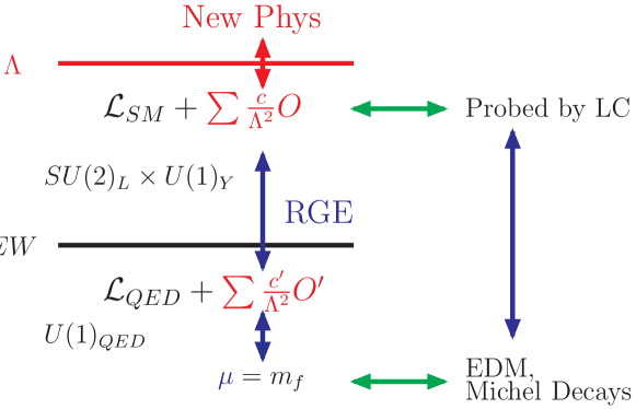
Figure 1: The connection between high and low energy interactions in effective field theory. The symmetry at each mass scale is given. All notations are given in the text.

A schematic representation of our approach is given in Fig.(1). Since the list of operators are known for some time; thus in that sense our approach is not new. However, a detail analysis the CPV effects incorporating RG effects have not been given before.

2 Dimension six operators

Without further ado we give the most general $SU(2)\times U(1)$ invariant Lagrangian with dimension six 4-lepton operators. We assume that there are no sterile neutrinos below $\Lambda$. In the weak basis they are not flavor diagonal and are given below:

$${\cal L}^{eff} = {\cal L}_{SM}+{\cal L}^{6}\,,$$

$${\cal L}^{6} = \sum\frac{c_{S}^{ij,kl}}{\Lambda^{2}}O_{S}^{ij,kl}+{\cal L}^{6}_{V}+h.c.$$ (1)

where

$$O_{S}^{ij,kl}=(\bar{L}_{ia}e_{j})(\bar{e}_{k}L_{la}),$$ (2)

and the vector like dimension-6 lagrangian is

$${\cal L}^{6}_{V} = \frac{c_{LL}^{ij,kl}}{\Lambda^{2}}(\bar{L}_{ia}\gamma^{\mu}L_{ja})(\bar{L}_{kb}\gamma_{\mu}L_{lb})+\frac{c_{LR}^{ij,kl}}{\Lambda^{2}}(\bar{L}_{ia}\gamma^{\mu}L_{ja})(\bar{e}_{k}\gamma_{\mu}e_{l})$$ (3)

$$+\frac{c_{RR}^{ij,kl}}{\Lambda^{2}}(\bar{e}_{i}\gamma^{\mu}e_{j})(\bar{e}_{k}\gamma_{\mu}e_{l})+\frac{d_{LL}^{ij,kl}}{\Lambda^{2}}\left(\bar{L}_{ia}\gamma^{\mu}L_{jb}\right)\left(\bar{L}_{kb}\gamma_{\mu}L_{la}\right)$$

$$+h.c.$$

The sum in Eq.(1) is taken over family indices denoted by $(i,j,k,l)$ and $SU(2)$ indices are $a,b$. $L_{i},e_{j}$ are $SU(2)$ lepton doublet and singlet respectively. All repeated indices are summed unless otherwise specified. Without knowledge of the new physics generating the operators $O_{S,V}$ the Wilson coefficients $c_{S,V},\ d_{LL}$ are unknown complex parameters. There are altogether $324$ parameters and a general analysis is not meaningful. They contain flavor changing neutral currents at the zeroth order. From the non-observation of rare muon or $\tau$ decays we learn that these terms are highly suppressed. This can be implemented by assuming that the Wilson coefficients of a given chiral structure denoted generically by $c^{ij,kl}$ is given by $c^{ij,kl}=(constant)\cdot\delta^{ij}\delta^{kl}$. This greatly simplifies the analysis and also makes the physics more transparent. A notable exception to this are the split fermion models in extra dimension as discussed in[10]. With this caveat in mind we can simplify Eq.(3) to

$${\cal L}_{V}^{6} = \frac{c_{LL}}{\Lambda^{2}}(\bar{L}_{ia}\gamma^{\mu}L_{ia})(\bar{L}_{kb}\gamma_{\mu}L_{kb})+\frac{c_{LR}}{\Lambda^{2}}(\bar{L}_{ia}\gamma^{\mu}L_{ia})(\bar{e}_{k}\gamma_{\mu}e_{k})$$ (4)

$$+\frac{c_{RR}}{\Lambda^{2}}(\bar{e}_{i}\gamma^{\mu}e_{i})(\bar{e}_{k}\gamma_{\mu}e_{k})+\frac{d_{LL}}{\Lambda^{2}}\left(\bar{L}_{ia}\gamma^{\mu}L_{ib}\right)\left(\bar{L}_{kb}\gamma_{\mu}L_{ka}\right)$$

$$+h.c.$$

As for the scalar coefficients in general they are not universal. The best known examples are the Yukawa couplings of the SM which are hierarchical and family dependent. We call this case type I scalar couplings. At the opposite end we have the simplifying case in which all $c_{S}$ have the same size will be referred to as type II scalar couplings. We use these two to illustrate the very different physics that they represent.

1. Type I scalar couplings
   

   Now ${\cal L}^{6}$ takes the simplified form

   $${\cal L}^{6}=\sum\frac{c_{S}^{ij,kl}}{\Lambda^{2}}O_{S}^{ij,kl}+\sum\frac{c_{V}}{\Lambda^{2}}O_{V}^{ij,kl}.$$ (5)

   where $c_{V}$ is a generic symbol for Wilson coefficients. Hermiticity demands that the Wilson coefficients associated with $O_{V}$ are all real. Now we can perform biunitary transformations to the mass eigenbasis of the charged leptons and neutrinos. It can be seen from Eqs.(4,5) when they are expanded the terms associated with the $c$’s are neutral current (NC) terms. Only $d_{LL}$ involves charged current (CC). The NC terms are flavor diagonal and their couplings are real. On the other hand the CC terms will be multiplied by the lepton mixing matrix, i.e. the PMNS matrix responsible for neutrino oscillations [7]. This is completely analogous to the SM where a phase of the weak charged current arises from fermion basis rotations and not the gauge coupling which is real. Next we examine the scalar terms.

   The same basis transformation will also multiply the $c_{S}$’s by the unitary matrices $U_{L}$ and $U_{R}$ which diagonalize $L_{i}$ and $e_{j}$. Let us denote the mass eigenstates by $L_{i}^{\prime}$ and $e^{\prime}_{j}$ respectively. Then the scalar part of Eq.(5) becomes

   $$\frac{c_{S}^{ij,kl}}{\Lambda^{2}}\left[\overline{L_{p}^{\prime}}(U_{L}^{\dagger})_{pi}(U_{R})_{jq}e^{\prime}_{q}\right]\left[\bar{e^{\prime}}_{r}(U_{R}^{\dagger})_{rk}(U_{L})_{ls}L^{\prime}_{s}\right]$$ (6)

   where we have omitted the $SU(2)$ indices and sum over repeated indices. Although the matrices $U_{R}$ and $U_{L}$ are not known beyond that they are unitary we can still extract some general properties from the above. The effective Lagrangian of Eq.(6) will lead to effective scalar charged currents as well as flavor changing neutral currents. Since the couplings remain complex they will induce TVNC in $\mu$ and $\tau$ leptonic decays as well as generating EDM for leptons. Of particular interest are the flavor diagonal NC terms. Let us study the term with only the electron whose family index is 1. In the mass basis, it is

   $$\frac{c_{S}^{ij,kl}}{\Lambda^{2}}\left[\overline{e_{L}}_{1}(U_{L}^{\dagger})_{1i}(U_{R})_{j1}e_{R1}\right]\left[\overline{e_{R}}_{1}(U_{R}^{\dagger})_{1k}(U_{L})_{l1}e_{L1}\right]+h.c.$$

   $$=\frac{c^{\prime 11,11}_{S}}{\Lambda^{2}}\overline{e_{L}}_{1}e_{R1}\overline{e_{R}}_{1}e_{1L}$$ (7)

   where we have used the same labels for mass and weak eigenstates in the above equation. Clearly the above 4-Fermi operator has a real coefficient. Similarly one can show that all terms of the form $(\overline{l_{Li}}l_{Rj})(\overline{l_{Rj}}l_{Li})$ where $i,j=e,\mu,\tau$ have real coefficients. Only terms of the form $(\overline{l_{Li}}l_{Ri})(\overline{l_{Rj}}l_{Lj})$ where $i\neq j$ can have complex couplings since they are not hermitian. We now arrive at a general conclusion that besides the phase in the PMNS matrix low energy CP violation must involve scalar currents. In the case of NC effects more than one family is necessary. This generalizes the expectation from the SM.

   To summarize we have shown that in going to the mass eigenbasis there is no loss of generality. The effective scalar Lagrangian for the terms which contain CP phases can be written as

   $${\cal{L}}_{s}=\sum\frac{c_{S}^{ii,jj}}{\Lambda^{2}}\overline{L_{i}}e_{Ri}\overline{e_{Rj}}L_{j}+h.c.$$ (8)

   and again for notational simplicity the prime on $c_{S}$ has been dropped. As for the vector coupling terms it is easy to see that going to the mass eigenbasis produces

   $${\cal{L}}_{V}^{6} = \frac{c_{LL}}{\Lambda^{2}}(\overline{\nu_{iL}}\gamma^{\mu}\nu_{iL}+\overline{e_{iL}}\gamma^{\mu}e_{iL})(\overline{\nu_{jL}}\gamma_{\mu}\nu_{jL}+\overline{e_{jL}}\gamma_{\mu}e_{jL})$$ (9)

   $$+ \frac{c_{LR}}{\Lambda^{2}}(\overline{\nu_{iL}}\gamma^{\mu}\nu_{iL}+\overline{e_{iL}}\gamma^{\mu}e_{iL})(\overline{e_{jR}}\gamma_{\mu}e_{jR})$$

   $$+ \frac{c_{RR}}{\Lambda^{2}}(\bar{e_{iR}}\gamma^{\mu}e_{iR})(\bar{e_{jR}}\gamma_{\mu}e_{jR})$$

   $$+ \frac{d_{LL}}{\Lambda^{2}}\left[(\overline{\nu_{iL}}\gamma^{\mu}\nu_{iL})(\overline{\nu_{jL}}\gamma_{\mu}\nu_{jL})+(\overline{e_{iL}}\gamma^{\mu}e_{iL})(\overline{e_{jL}}\gamma_{\mu}e_{jL})+2V_{ij}V^{\dagger}_{kl}(\overline{\nu_{iL}}\gamma^{\mu}e_{jL})(\overline{e_{kL}}\gamma_{\mu}\nu_{lL})\right]$$

   $$+ h.c.$$

   where we are in the mass eigenbasis and $V$ is the PMNS matrix. For notational simplicity we retain the label of the weak basis. From the above equation we can see that the only physical phase is in the $CC\times CC$ terms. The coefficient is a product of the PMNS matrix element and a complex number $d_{LL}$. On the other hand in the $NC\times NC$ channels there are no phases and they also conserve flavor. We see from Eqs.(8) and (9) that the rare decay $\mu\rightarrow e\gamma$ is induced at 2-loops. This will be reserved for further studies. Hence our scenario is a very modest extension of SM expectations.

2. Type II scalar couplings
   The parameters $c_{S}^{ij,kl}$ are now independent of the family indices and can be taken out of the sum. A rotation to the mass eigenbasis and hermiticity produce only real coupling for $c_{S}$. We can now perform a Fierz transformation and $O_{S}$ becomes $(\bar{L_{i}}\gamma^{\mu}L_{i})(\bar{e_{j}}\gamma_{\mu}e_{j})$ and with only real couplings. This will modify the overall strengths of the right-handed lepton NC couplings but it does not give rise to TVNC. The strength of the charged current will be modified as in the previous case. We shall see later that lepton EDM will also not be generated up to two loops. Hence, this scenario of extreme simplification is phenomenologically not interesting and no detail discussion for it will be given.

We note in passing that a possible tensor term $O_{T}=(\bar{L}\sigma^{\alpha\beta}e)(\bar{e}\sigma_{\alpha\beta}L)$ is identically zero independent of the family indices states. Such terms can only be generated after electroweak symmetry breaking and are expected to be highly suppressed. The same is true when $e$ is replaced by a light sterile neutrino $\nu_{r}$. However, there are now more operators similar to ones we are studying that one can construct. We list them in [8]. Since there is no compelling evidence for light sterile neutrinos we shall not pursue them further.

Before we proceed we comment on the other dimension six operators involving gauge bosons and Higgs fields (see [5]). An example is the operator $O_{h}=\,\phi\bar{L}\sigma^{\alpha\beta}eW_{\alpha\beta}$ where $\phi$ is the Higgs doublet and $W_{\alpha\beta}$ is the field strength tensor of $SU(2)$. These operators are important in discussing electroweak breaking and a detail study can be found in [9]. In most models such an operator is generated at 1-loop or higher and thus more suppressed than the four fermion operators which can usually be generated at tree level. Examples can be found in models of extra dimensions [10] where $\Lambda$ is given by the mass of Kaluza-Klein modes and left-right symmetric models. Alternatively one can regard our approach to be the ansatz of 4-Fermi dominance below $\Lambda$.

3 1-loop renormalization of ${\cal L}^{6}$

The operators $O_{S,V}$ which we shall generically denote by $O^{6}_{A}$ are bare operators. Upon renormalization the operators will mix via

$$O^{6}_{A}=\sum_{B=1}^{5}Z^{-1}_{AB}(Z_{L})^{n/2}{Z_{e}}^{m/2}\,O^{6}_{Br}$$ (10)

where $Z_{L}$ and $Z_{e}$ are the wavefunction renormalization constants for the $L$ and $e$ fields and $n,m$ are the number of such fields in each of the $O_{i}$ operators. Hence $n,m=0,2,{\mathrm{or}}\ 4$. The sum here runs over the five terms of $O_{S}$ and $O_{V}$ and subscript $r$ denotes renormalized quantity. These five 4-fermi operators form a complete set at the 1-loop level in the limit that we can neglect lepton masses. The renormalized operator $O^{6}_{B,r}$ will depend on the t’Hooft renormalization scale $\mu$ whereas the bare operators do not. Correspondingly the $\mu$-dependence of the Wilson coefficients will be such to render the renormalized effective Lagrangian ${\cal L}^{6}_{r}$ independent of $\mu$. This leads to the renormalization group equation for the coefficients in Eqs.(1,3):

$$\mu\frac{d}{d\mu}c_{A}+\sum_{B}\gamma_{AB}c_{B}=0$$ (11)

where $\gamma_{AB}$ is the anomalous dimension matrix which is non-diagonal. The values of $c_{A}$ at the weak scale $v$ are obtained by solving the above equation plus boundary conditions which are the values given at another scale say at a few TeV where they will optimistically be measured in the future. Presently we only have limits on a few $c_{A}$ at the weak scale taken from searches at LEP II. We now return to discuss $\gamma_{AB}$ calculation.

Between the scales $\Lambda$ and $v$ the 1-loop renormalization of the operators $O_{A}$ are induced by the exchange of SM gauge bosons. We can ignore the Higgs boson contribution since the Yukawa couplings of the leptons are known to be small. The task at hand is to calculate the Feynman graphs listed in Fig.(2). Diagrams Fig. 2a and 2b are cancelled by the wave function renormalization graphs (not shown) for the vector coupling case. For scalar couplings the wavefunction renormalizations have to be included. Together with the remaining four diagram will give the total contribute to the anomalous dimension.

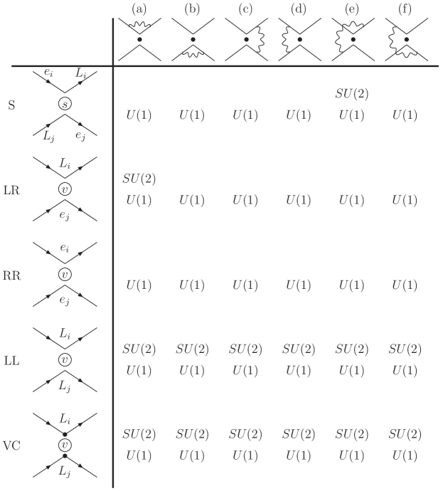
Figure 2: The first column gives the dimension 6 operators. The top row depicts their l-loop corrections. The entries in the table are the gauge bosons type given by the wavy lines. $L$ and $e$ represent the $SU(2)$ doublet and singlet fields respectively.

At the 1-loop level operators of the form $O_{h}$ are also generated. Figure (3) depicts two representative diagrams.

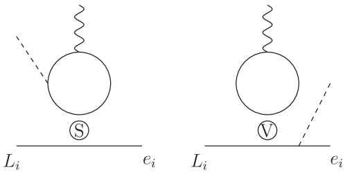
Figure 3: Representative diagrams of dipole operators generated from the SM and ${\cal L}^{6}$. The dash line denotes Higgs fields.

Obviously, they are proportional to lepton Yukawa couplings and can be neglected. In this limit, the four fermion operators, $O_{A}$, form a complete set under renormalization to this order. Thus, the form of Eq.(1) remains valid at the weak scale.

A standard calculation of the graphs depicted in Fig. 2 gives the following result for $\gamma_{AB}$ :

$$\gamma_{AB}=\frac{1}{4\pi}\left(\begin{array}[]{ccccc}-6\alpha_{1}&0&0&0&0\\ 0&-6\alpha_{1}&0&0&0\\ 0&0&12\alpha_{1}&0&0\\ 0&0&0&3(\alpha_{1}-\alpha_{2})&8\alpha_{2}\\ 0&0&0&6\alpha_{2}&3\alpha_{1}-7\alpha_{2}\end{array}\right)$$ (12)

in the basis of operators linked to $(c_{S},c_{LR},c_{RR},c_{LL},d_{LL})$ and $\alpha_{1}$. $\alpha_{2}$ are the fine structure constants for the $U(1)$ and $SU(2)$ respectively. This structure holds true for both type I and II scalar couplings. The difference being that in Type I $c_{S}$ is a 3$\times$3 matrix whereas it is just one parameter for type II.

Below the EW scale the running of the coefficients are governed by QED corrections only. This is described by the known $\beta$ functions for the running of $\alpha_{1}$ and $\alpha_{2}$.

The RGE for $c_{S}$ and $c_{LR}$ can be solved analytically as they are controlled by $U(1)$. First we define the quantities

$${\cal G}_{S}(\mu)\equiv{C_{S}(\mu)\over C_{S}(M_{Z})}\,,\;{\cal G}_{LR}(\mu)\equiv{C_{LR}(\mu)\over C_{LR}(M_{Z})}$$ (13)

and obtain the result

$${\cal G}_{S}(\mu)={\cal G}_{LR}(\mu)=\left({\alpha_{1}(M_{Z})\over\alpha_{1}(\mu)}\right)^{-\frac{30}{41}}\,.$$ (14)

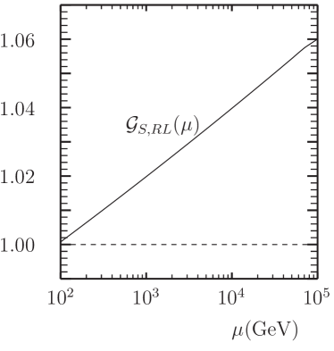
Figure 4: The running of ${\cal G}(\mu)$ defined in the text.

As can be seen from Fig.(4), numerically the RG effect is not significant. Even for $\Lambda=10$ TeV it gives a $\sim 4\%$ correction. The running from weak scale down is also not very large and is controlled by the well known $\beta_{QED}$ [11]. Including that we find that the Wilson coefficient for the scalar operator increases by 10% in going from the scale of muon mass to 1 TeV.

4 Lepton EDM from 4-Fermi Interactions

Next we determine whether ${\cal L}^{6}$ will generate an EDM at the 1-loop level. As a prelude we first determine how Eq.(8) is related to the lepton masses. Clearly the 4-fermi scalar iterations can lead to a mass at 1-loop via Fig.(5).

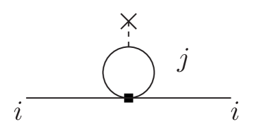
Figure 5: 1-loop fermion mass from scalar 4-fermion interactions.

Moreover, in the mass basis there are no off diagonal contributions. Then the physical mass of a lepton is given by

$$\frac{m_{i}}{v}=y_{i}+\frac{1}{8\pi^{2}}\sum_{j}c_{S}^{ii,jj}y_{j}$$ (15)

where $y_{i}$ is the Yukawa coupling of the SM. The first term is the SM contribution. Ignoring the case of fine tuning between the two terms we expect the real part of $c_{S}^{ii,jj}$ to scale like $m_{i}/m_{j}$. In particular for the electron we expect $c_{S}^{ee,\tau\tau}\sim m_{e}/m_{\tau}$ and $c_{S}^{ee,\mu\mu}\sim m_{e}/m_{\mu}$. Similarly for the muon. Notice that for the $\tau$ the main contribution comes from the diagonal coupling $c_{S}^{\tau\tau,\tau\tau}$ which can be of order unity. We note that Eq.(15) there are no flavor changing scalar NC in the mass eigenbasis.

Proceeding to the calculation of EDM, we observe that at 1-loop there are two possible ways for a 4-fermion operator to combine with the SM to give rise to an EDM, see Fig.6.

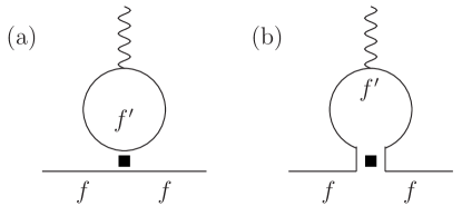
Figure 6: The 2 possible ways for a 4-fermion operator to generate EDM. The black box denotes any 4-fermi coupling which is complex.

Now we shall show neither of them leads to EDM. It is more convenient to work in the mass basis. As seen from Fig.(6a) the internal line $f^{\prime}$ must be a charged lepton. This narrows the list of contributing operators to the NC type. We saw in Sec.2 that the only complex couplings are the ones associated with the scalar operators $(\overline{f_{L}}f_{R})(\overline{f^{\prime}_{R}}f^{\prime}_{L})$ with $f\neq f^{\prime}$. An elementary calculation shows that Fig.(6a) gives zero contribution. Now we turn to Fig.(6b) which does not involve a trace. This comes from operators of the form $(\overline{f_{L}}f^{\prime}_{R})(\overline{f^{\prime}_{R}}f_{L})$. A Fierz transformation turns this into one associated with $c_{LR}$. This coefficient is real coefficient and thus not contribute to EDM. For the case $f=f^{\prime}$ this Wilson coefficients are real. Thus, we conclude that there is no 1-loop EDM with purely leptonic 4-fermi operators. We proceed to consider 2 loops.

The Feynman diagrams we need to consider are given by Fig.7.

Figure 7: EDM generated by 4-fermion operator at the 2-loop level.

Only the coupling $c_{S}$ represented by the black square can contribute. The internal wavy line indicates photon exchange and other gauge bosons exchanges are suppressed. The diagrams are logarithmically divergent due to the point coupling. One can regulate this by substituting $1/\Lambda^{2}\rightarrow 1/(q^{2}-\Lambda^{2})$ where $q$ is the loop momentum carried by the internal photon. This dampens the high frequency modes of the integration and also reproduces the point coupling at low energies. Alternatively, one can simply cut off the integral at $\Lambda$. We have checked that both ways give the same leading result. The EDM $d_{l}$ of a charged lepton $l=e,\mu$ or $\tau$ is given by

$$d_{f}={e\alpha\over 16\pi^{3}}\sum_{i}{m_{i}\mathbf{Im}c^{ff,ii}_{S}\over\Lambda^{2}}{\cal F}\left({m_{i}^{2}\over\Lambda^{2}}\right)\,,$$ (16)

and the function

$${\cal F}(x) = \int^{1}_{0}{d\lambda\lambda(1-\lambda)\over x-\lambda(1-\lambda)}\ln\frac{x}{\lambda(1-\lambda)}$$

$$= \mbox{Re}\left\{{1\over\sqrt{1-4x}}\left[\ln x\ln{\sqrt{1-4x}-1\over\sqrt{1-4x}+1}\right.\right.$$

$$+ \left.\left.Li_{2}\left({2\over 1-\sqrt{1-4x}}\right)-Li_{2}\left({2\over 1+\sqrt{1-4x}}\right)\right]\right\}\,,$$

$${\cal F}(x\ll 1) \sim -(2+\ln x)\,,$$ (18)

where $i=e,\mu,\tau$. There are two helicity flips in the above result. The first one involves the scalar 4-fermi interactions $c_{s}$ which we have argued before the modulus of which contains a mass factor $m_{i}$. The second one is the helicity flip of the fermion in the loop which is explicit in Eq.(16). As expected, in the limit of massless fermions there is no EDM.

The muon and electron EDM’s will be dominated by the diagram with the $\tau$ running in the loop, and the result can be expressed as

$$d_{f}\sim 5.88\times 10^{-24}\ \mathbf{Im}c^{ff,\tau\tau}_{S}\left({1\mbox{TeV }\over\Lambda}\right)^{2}(\mbox{e-cm})\,.$$ (19)

As expected $d_{l}$ vanishes when the new physics scale becomes arbitrarily high and if the SM symmetry remains good.

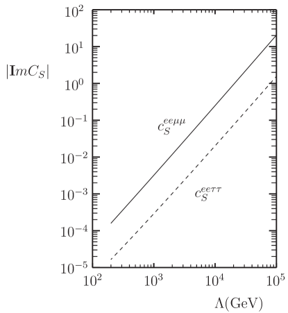
Figure 8: The upper limit of the imaginary part of $c_{S}$ derived from the electron EDM.

For the electron, experimentally we have $|d_{e}|<1.7\times 10^{-27}(\mbox{e-cm})$ [12] from which we derive an upper limit for $|\mathbf{Im}c^{ee,\tau\tau}_{S}|<3\times 10^{-4}(\Lambda/1\mbox{TeV})^{2}$. This in turn can be used to constrain the CP violating leptonic decays for the $\tau$. Similarly barring possible cancellations, the electron EDM can also set an upper bound on the coefficient $|\mathbf{Im}c^{ee,\mu\mu}_{S}|<3.3\times 10^{-3}(\Lambda/1\mbox{TeV})^{2}$. This we shall use later to limit effects of CP violation in muon decay spectrum. Figure (8) shows our result from the electron EDM study.

Similarly, for the $\tau$ EDM, the muon in the loop dominates, and

$$d_{\tau}\sim 5.34\times 10^{-25}\mathbf{Im}c^{\tau\tau,\mu\mu}_{S}\left({1\mbox{TeV }\over\Lambda}\right)^{2}(\mbox{e-cm})\,.$$ (20)

The EDM’s can certainly receive a tree level contribution from the dimension six dipole operators : $\frac{c_{d1}^{ij}}{\Lambda^{2}}\bar{L}^{i}\sigma^{\mu\nu}e^{j}B_{\mu\nu}\phi$ and $\frac{c_{d2}^{ij}}{\Lambda^{2}}\bar{L}^{i}\sigma^{\mu\nu}e^{j}W_{\mu\nu}\phi$, where $\phi$ is the Higgs field, and $W_{\mu\nu}$ and $B_{\mu\nu}$ are the $SU(2)$ and $U(1)_{Y}$ field strength respectively. After electroweak symmetry breaking, i.e. $\phi\rightarrow v/\sqrt{2}\,(0,1)^{T}$, this will contribute to EDM and $g-2$ of the lepton at the tree level. We estimate that the experimental bounds are $\left|{\mathbf{Im}}[\cos\theta_{W}c_{d1}^{ee}+\sin\theta_{W}c_{d2}^{ee}]\right|<2.4\times 10^{-10}$ from $d_{e}$ and $\left|{\mathrm{Re}}[\cos\theta_{W}c_{d1}^{ee}+\sin\theta_{W}c_{d2}^{ee}]\right|<7.1\times 10^{-6}$ from $a_{e}$ for $\Lambda=1$ TeV. The limit from the muon anomalous moment is about one order of magnitude better. . We interpret this to imply that the UV completed theory will either gives a small phase to this operator and/or it arises from 2 or higher loops with possibly other dynamical suppression factors.

For completeness we note that the RG running of the dimension-6 electric dipole operators below the EW scale is not very significant [11] and they are not included in this estimate.

5 More Phenomenological Implications

5.1 CP violating Michel parameter in $\mu$ decays

In the muon decay, $\mu\rightarrow e\nu_{\mu}\bar{\nu}_{e}$, the electron polarization $\overrightarrow{P_{e}}$ is

$$\overrightarrow{P_{e}}=P_{L}\hat{z}+P_{T1}{(\hat{z}\times\overrightarrow{P}_{\mu})\times\hat{z}\over|(\hat{z}\times\overrightarrow{P_{\mu}})\times\hat{z}|}+P_{T2}{\hat{z}\times\overrightarrow{P}_{\mu}\over|\hat{z}\times\overrightarrow{P_{\mu}}|}$$ (21)

where $\overrightarrow{P}_{\mu}$ is the muon polarization vector and $\hat{z}$ is the unit vector in the electron momentum direction. The $P_{T2}$ term is a T-violating observable. To compare with the experimental results we follow the convention used by [13] to describe the general decay matrix elements, namely,

$${4G_{F}\over\sqrt{2}}\sum_{E,M=R,L}^{\gamma=S,V,T}g^{\gamma}_{EM}\left\langle\bar{e}_{E}|\Gamma^{\gamma}|\nu_{e}\right\rangle\left\langle\bar{\nu_{\mu}}|\Gamma_{\gamma}|\mu_{M}\right\rangle$$ (22)

where $E,M$ are the chiralities of electron and muon respectively.

The upper limit of $P_{T2}$ [14], can be translated into bounds on two CP-odd parameters $\alpha^{\prime}=-0.003(69)$ and $\beta^{\prime}=0.024(101)$ which are defined as:

$$\alpha^{\prime} = 8Im\left\{g^{V}_{LR}(g^{S*}_{RL}+6g_{RL}^{T*})-g^{V}_{RL}(g^{S*}_{LR}+6g_{LR}^{T*})\right\}\,,$$

$$\beta^{\prime} = 4Im\left\{g^{V}_{RR}g^{S*}_{LL}-g^{V}_{LL}g^{S*}_{RR}\right\}\,.$$ (23)

The assumption that the SM gauge symmetry is valid up to $\Lambda$ leads to $g^{V}_{RR}=g^{V}_{LR}=g^{V}_{RL}=0$ automatically. This is consistent with the latest precision measurement of muon decays [15]. The only new contribution comes from $g^{S}_{RR}$. Since the correction is small we can normalize the rate to $G_{F}$; thus, we set $g^{V}_{LL}=1$. We predict $\alpha^{\prime}=0$ and

$$\beta^{\prime}=4Img^{S}_{RR}={\sqrt{2}\over G_{F}\Lambda^{2}}\mbox{Im}\,c_{S}^{\mu\mu ee}\,.$$ (24)

From the electron EDM we already have $|\beta^{\prime}|<4.0\times 10^{-4}$ for $\Lambda=1$ TeV. This is two orders of magnitude below the anticipated sensitivity of the current PSI experiment.

It is interesting to note that $\mbox{Re}\,c_{S}^{\mu\mu ee}$ is probed by measuring two other Michel parameters $\eta$ and $\xi$. The current limit [13] translates into $|c_{S}^{\mu\mu ee}|<2.2$ which is not very stringent as compared from the EDM limit.

5.2 CP violation in $e^{+}e^{-}\rightarrow\tau^{+}\tau^{-}$ at the Linear Collider

With the upper bound obtained from EDM we can now estimate the size of CP violating signatures in a purely leptonic flavor conservation reaction such as $e^{+}(p_{+})e^{-}(p_{-})\rightarrow\tau^{+}(k_{+})\tau^{-}(k_{-})$ where the 4-momentum of each particle are given in the corresponding bracket. We look for a signal that will be directly sensitive to $ImC_{S}$. The signal will involve measuring the polarization of a final state $\tau$ in the triple product such as $(\hat{p}_{-}+\hat{k}_{-})\cdot(\vec{s}_{e}\times\vec{s}_{\tau})$ where $\hat{p}_{-}$ is the unit 3-vector along the incoming $e^{-}$ direction, $\hat{k}_{-}$ is the unit 3-vector along the outgoing $\tau^{-}$ direction, $\vec{s}_{e}$ is the polarization of incoming electron beam, and $\vec{s}_{\tau}$ is the polarization 3-vector of the $\tau^{-}$ all in the center of mass system. Usually $\vec{s}_{e}$ is taken to be either longitudinally or transversely polarized.

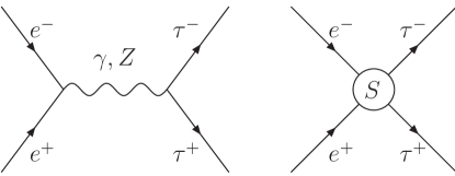
Figure 9: The tree level Feynman diagrams for the CP violating signature in LC.

This signature arises from the interference of an SM amplitude and the 4-fermi term as depicted in Fig.(9). It is straightforward to calculate the T-odd (TO) invariant amplitude and we obtain

$$|M_{TO}|^{2}=\frac{s}{24e^{2}\Lambda^{2}}ImC_{s}^{ee,\tau\tau}(\hat{p}_{-}+\hat{k}_{-})\cdot(\vec{s}_{e}\times\vec{s}_{\tau})$$ (25)

where we have scaled by the strength of the QED term and $s$ is the cm energy square. The linear dependence on $s$ is characteristic of point interactions. This triple correlation is directly related to EDM measurement. This can be easily understood since the diagrams of Fig.(9) are the ones obtained from cutting the 2-loop EDM diagram with amputated photon. Consequently we obtain an upper bound on the coefficient to be $10^{-4}(\frac{\sqrt{s}}{1\mathrm{TeV}})^{2}$. The corresponding quantity using muons will be an order of magnitude higher due to the less stringent bound on $c_{S}^{ee,\mu\mu}$ (see Fig. 8).

In passing we note that other triple correlations involving two $\tau$ spins are highly suppressed by $m_{e}$ and $m_{\tau}$ and will not be a good signature to probe CPV in contact interactions. This is not the case for $\tau$ weak dipole moments searches [16]. The contribution of weak dipole moments are very small for us. We have also not included the unitarity phase from the SM which can be calculated precisely including the sign (see [17]).

6 Conclusions

Starting from the assumption that the SM gauge symmetry is valid from the weak scale to some new physics scale $\Lambda$ and the matter content of the SM we have shown that the general set of dimension six leptonic 4-fermi operators can be cast into mass eigenbasis without lost of generality. This assumption also reduces the number of 4-Fermi operators as compared with the usual assumption of only $U(1)_{em}$ as the good symmetry. We then assume that the vector Wilson coefficients of a given chiral structure are constants. This eliminates zeroth order FCNC. Then the most interesting non-standard Lorentz structures are the scalar charged and neutral current interactions. The overall 4-Fermi coupling will also be renormalized due to the addition of the $d_{LL}$ term. There are also modifications of the SM $V,A$ structure to the neutral currents which can be read from Eq.(9). However, due to the high value of $\Lambda$ these corrections are within the current bounds. More interestingly we find that the only possible new CP violating terms are the scalar Wilson coefficients for $(\bar{L_{i}}e_{i})(\bar{e}_{j}L_{j})$ with different family indices $i\neq j$. We use the renormalization group equations to run the Wilson coefficients at the scale $\Lambda$ to the weak scale and further down to lower energies of the lepton masses. We found that there is a 10% correction to the magnitude of these operators.

The new phase of the coefficient $c_{S}^{ii,jj}$ will induce EDM of charged leptons at the 2-loop level. The constraint from the electron EDM is currently the most stringent limit on $c_{S}^{ee,jj}/\Lambda^{2}$ where $j=\mu,\tau$. This in turn implies that CP violation signature will be too small to be detected in measurements of the electron spectrum in $\mu$ decays.

At high energies CP violation can occur in $e^{+}e^{-}\rightarrow\tau^{+}\tau^{-}$ at the linear collider by measuring the triple correlation $(\hat{p}_{-}+\hat{k}_{-})\cdot(\vec{s}_{e}\times\vec{s}_{\tau})$. From EDM we estimated the upper limit of this signature to be $\lesssim 10^{-4}$ making this almost impossible to measure. The case for muons is more promising but still very challenging. We note that CP violation signatures at colliders are a new way of studying the phenomenon. However it is an endeavor that requires very high precision at least in the scenario of 4-fermi operator dominance.

Our analysis is general and independent of the details of the unknown new physics. We have made very conservative assumptions. If there are new states found between $\Lambda$ and $v$ our analysis will not apply. An example will be the existence of sterile neutrinos below $\Lambda$. As seen from the list given in [8] the loop calculation of the EDM will have to be altered although the RG considerations suffer little change. On the other hand discovering more Higgs particles will not alter our analysis below $v$ . Their effects can be incorporated into the effective scalar couplings. This study demonstrates quantitatively the complementarity of high energy and precision low energy measurements as probes of new physics. This kind of relations are quite general and are expected to exist in many models. It can be extended to include 4-Fermi operators with quarks and we will leave this for a future study.

Note added: After the completion of this work, the paper of Cirigliano el al [18] was brought to our attention. The authors used similar effective operator analysis to address the problem of lepton flavor violation and its connection to neutrino mass generation. Since they are primarily interested in decays such as $\mu\rightarrow e\gamma$, the dimension six operators analyzed contain two lepton fields whereas we analyzed the four lepton terms. The dipole operators play an important role in their work in contrast to ours as we are interested in the problem of EDM’s. They also do not consider RG running of the Wilson coefficients. The importance of a general analysis of dimension six operators respecting gauge symmetry of the SM in studies of new physics in the lepton is recognized and exploited by both of us in a different but complementary ways.