July 2005

Electromagnetic corrections
to non-leptonic two-body $B$ and $D$ decays

Elisabetta Baracchini¹ and Gino Isidori²

${}^{1}~{}$ Dipartimento di Fisica, Universitá di Roma “La Sapienza” and
INFN, Sezione di Roma, P.le A. Moro 2, I-00185 Roma, Italy

${}^{2}~{}$INFN, Laboratori Nazionali di Frascati, I-00044 Frascati, Italy

Abstract

We present analytic expressions to evaluate at ${\cal O}(\alpha)$ the effects of soft-photon emission, and the related virtual corrections, in non-leptonic decays of the type $B,D\to P_{1}P_{2}$, where $P_{1,2}$ are scalar or pseudoscalar particles. The phenomenological implications of these results are briefly discussed. For $B$ decays into charged pions the effects of soft-photon emission are quite large: the corrections to the rates can easily exceed the $5\%$ level if tight cuts on the photon energy are applied.

1 Introduction

The large amount of data collected at $B$ factories has allowed to reach statistical accuracies of the order of a few percent on the measurements of several $B$ meson branching fractions. At this level of accuracy electromagnetic effects cannot be neglected. On the one hand, in order to ensure a good control of the experimental efficiencies, it is necessary to include in Montecarlo simulations the unavoidable emission of soft photons that accompanies all processes with charged particles. On the other hand, the effective cuts applied on the (soft) photon spectra are a key information for a meaningful comparison between theory and experiments.

The theoretical treatment of the infrared singularities generated within QED is a well known subject and one of the pillars of quantum field theory. A clear and very general discussion can be found, for instance, in the classical papers [1, 2]. The general properties of QED have been exploited in great detail in the case of genuine electroweak processes, or processes which can be fully described within perturbation theory within the Standard Model (SM). In these cases there exist both precise theoretical calculations of the electromagnetic (e.m.) corrections and accurate Montecarlo programs which include the effects of soft photon emission, such as PHOTOS [3]. Similar tools have not been developed for most exclusive hadronic processes and, in particular, for $B$ and $D$ decays.

Recently, the issue of electromagnetic corrections have received considerable attention in the context of kaon physics [4, 5, 6, 7]. As discussed in these works, and as confirmed by recent experimental analyses [8], a correct simulation of electromagnetic corrections is a key ingredient for a precise determination of $V_{us}$ and other effective couplings of weak interactions.

The purpose of the present work is to present simple analytic formulae for he theoretical evaluation, and the numerical simulation, of the leading radiative corrections in $B$ or $D$ meson decays into two scalar or pseudoscalar particles. Given the universal character of the infrared singularities, we evaluate the effects of soft photon emission (and the corresponding virtual corrections) within scalar QED and in the approximation of a point-like effective weak vertex. The results thus obtained are valid up to constant ${\cal O}(\alpha)$ terms (not enhanced by large logs) related to the matching between this effective theory and the “true” theory where the dynamical aspects of weak interactions are taken into account. Moreover, our calculation does not take into account the possible ${\cal O}(E_{\gamma})$ terms associated to non-bremsstrahlung amplitudes (hard photon emission).

2 Photon-inclusive widths

The most convenient infrared-safe observable related to the process $H\to P_{1}P_{2}$ is the photon-inclusive width

$$\Gamma^{\rm incl}_{12}(E^{\rm max})=\left.\Gamma(H\to P_{1}P_{2}+n\gamma)\,\right|_{\sum E_{\gamma}<E^{\rm max}}~{},$$ (1)

namely the width for the process $H\to P_{1}P_{2}$ accompanied by any number of (undetected) photons, with total missing energy less or equal to $E^{\rm max}$ in the $H$ meson rest frame. At any order in perturbation theory we can decompose $\Gamma^{\rm incl}_{12}$ in terms of two theoretical quantities: the so-called non-radiative width, $\Gamma^{0}_{12}$, and the corresponding energy-dependent e.m. correction factor $G_{12}(E^{\rm max})$,

$$\Gamma^{\rm incl}_{12}(E^{\rm max})=\Gamma^{0}_{12}~{}G_{12}(E^{\rm max})~{}.$$ (2)

The energy dependence of $G_{12}(E)$ is unambiguous and universal (i.e. independent from the short-distance dynamics which originate the decay) up to terms which vanish in the limit $E\to 0$. On the contrary, the normalization of $G_{12}(E)$ is arbitrary: we can always move part of the finite (energy-independent) electromagnetic corrections from $\Gamma^{0}_{12}$ to $G_{12}(E)$. Only the product in (2) corresponds to an observable quantity.

In the following we report the explicit expressions of $G_{12}(E)$ as obtained by means of a scalar-QED calculation at ${\cal O}(\alpha)$. In order to treat separately infrared (IR) and ultraviolet (UV) divergences, we regulate the former by means of a photon mass and the latter by means of dimensional regularization. We then renormalize the point-like weak coupling in the $\overline{\rm MS}$ scheme.

By construction, we define the non-radiative amplitude $\Gamma^{0}_{12}$ as follows

$$\Gamma^{0}_{12} = \frac{\beta}{16\pi M_{H}}\left|{\cal A}_{H\to P_{1}P_{2}}(\mu)\right|^{2}~{},$$ (3)

$$\beta^{2} = \left[1-\left(r_{1}+r_{2}\right)^{2}\right]\left[1-\left(r_{1}-r_{2}\right)^{2}\right]~{},\qquad r_{i}~{}=~{}\frac{M_{i}}{M_{H}}~{},$$ (4)

namely the tree-level rate expressed in terms of the renormalized weak coupling. With this convention, the function $G_{12}(E)$ can be written as

$$G_{12}(E)=1+\frac{\alpha}{\pi}\left[b_{12}\ln\left(\frac{M_{H}^{2}}{4E^{2}}\right)+F_{12}+\frac{1}{2}H_{12}+N_{12}(\mu)\right]~{},$$ (5)

where, following the notation of Ref. [4], we have denoted by $H_{12}$ the finite term arising from virtual corrections, and by $F_{12}$ the energy-independent term generated by the real emission:

$$\int_{E_{\gamma}<E}~{}\frac{d^{3}\vec{k}}{(2\pi)^{3}~{}2E_{\gamma}}~{}\sum_{\rm spins}\left|\frac{{\cal A}(H\to P_{1}P_{2}\gamma)}{{\cal A}(H\to P_{1}P_{2})}\right|^{2}=~{}\frac{\alpha}{\pi}\left[b_{12}\ln\left(\frac{m^{2}_{\gamma}}{4E^{2}}\right)+F_{12}+{\cal O}\left(\frac{E}{M_{H}}\right)\,\right]~{}.$$ (6)

As expected, after summing real and virtual corrections the infrared logarithmic divergence cancel out in $G_{12}(E)$, giving rise to the universal $\ln(M_{H}/E)$ terms proportional to

$$b_{+-} = \frac{1}{2}-\frac{4-\Delta_{1}^{2}-\Delta_{2}^{2}+2\beta^{2}}{8\beta}\,\ln\left({\frac{\Delta_{1}+\beta}{\Delta_{1}-\beta}}\right)\quad+\quad(1\to 2)~{},$$

$$b_{\pm 0} = 1-\frac{\Delta_{1}}{2\beta}\,\ln\left({\frac{\Delta_{1}+\beta}{\Delta_{1}-\beta}}\right)~{},$$ (7)

where $\Delta_{1(2)}=1+r_{1(2)}^{2}-r_{2(1)}^{2}$.

Note that $G_{12}(E)$ does depend explicitly on the ultraviolet renormalization scale $\mu$. The scale dependence contained in $N_{12}(\mu)$ cancels out only in the product $\Gamma^{0}_{12}~{}G_{12}(E)$ due to the corresponding scale dependence of the weak coupling. As we shall discuss in more detail later on, in practice we are not able to exploit the numerical consequences of this cancellation due to the absence of a first-principle calculation of ${\cal A}_{H\to P_{1}P_{2}}(\mu)$.

In the $H^{0}\to P_{1}^{+}P^{-}_{2}$ case we find the following explicit expressions for the coefficients in eq. (5):

$$F_{+-} = \frac{\Delta_{1}}{2\beta}\ln\left(\frac{\Delta_{1}+\beta}{\Delta_{1}-\beta}\right)+\frac{4-\Delta_{1}^{2}-\Delta_{2}^{2}+2\beta^{2}}{4\beta}\left[\,f\left(-\frac{\beta}{\Delta_{1}}\right)-\,f\left(\frac{\beta}{\Delta_{1}}\right)\right.$$ (8)

$$-\frac{1}{2}\,f\left(\frac{\Delta_{1}-\beta}{2\Delta_{1}}\right)+\frac{1}{2}\,f\left(\frac{\Delta_{1}+\beta}{2\Delta_{1}}\right)+\frac{1}{2}\,\ln\left(2\right)\ln\left(\frac{\Delta_{1}-\beta}{\Delta_{1}+\beta}\right)$$

$$\left.+\frac{1}{4}\,\ln^{2}\left(1+\frac{\beta}{\Delta_{1}}\right)-\frac{1}{4}\,\ln^{2}\left(1-\frac{\beta}{\Delta_{1}}\right)\right]\quad+\quad(1\to 2)$$

$$H_{+-} = \frac{4-\Delta_{1}^{2}-\Delta_{2}^{2}+2\beta^{2}}{8\beta}\left[{\pi}^{2}+2f\left(\frac{\Delta_{1}+\beta}{2\beta}\right)-2f\left(-\frac{\Delta_{1}-\beta}{2\beta}\right)\right.$$ (9)

$$\left.+\ln^{2}\left(\Delta_{1}-\beta\right)-\ln^{2}\left(\Delta_{1}+\beta\right)+2\ln\left({\frac{\Delta_{1}-\beta}{\Delta_{1}+\beta}}\right)\ln\left(\frac{\beta}{2}\right)\right]-2\,\ln\left(2\right)$$

$$+1+\frac{1}{2}\,\beta\,\ln\left({\frac{\Delta_{1}+\beta}{\Delta_{1}-\beta}}\right)+\frac{1}{2}\,\left(1+\Delta_{1}\right)\ln\left({\Delta_{1}}^{2}-{\beta}^{2}\right)\quad+\quad(1\to 2)\quad$$

$$N_{+-} = \frac{3}{4}\ln\left(\frac{\mu^{2}}{M^{2}_{H}}\right)-\frac{3}{4}\ln(r_{1}^{2})\quad+\quad(1\to 2)~{},$$ (10)

where

$$f(x)={\rm Re}[{\rm Li}_{2}(x)]=-\int_{0}^{x}\frac{dt}{t}\ln|1-t|~{}.$$ (11)

In the $H^{\pm}\to P_{1}^{\pm}P^{0}_{2}$ case we find:

$$F_{\pm 0} = 1+\,\frac{\Delta_{1}}{2\beta}\ln\left({\frac{\Delta_{1}+\beta}{\Delta_{1}-\beta}}\right)-\frac{\Delta_{1}}{4\beta}\,\left[\ln^{2}\left({\frac{\Delta_{1}-\beta}{\Delta_{1}+\beta}}\right)+4\,f\left({\frac{2\Delta_{1}}{\Delta_{1}+\beta}}\right)\right]$$ (12)

$$H_{\pm 0} = -\frac{\Delta_{1}}{\beta}\left[\frac{1}{2}\ln^{2}\left(\Delta_{1}+\beta\right)-\frac{1}{2}\ln^{2}\left(\Delta_{1}-\beta\right)+f\left(\frac{\Delta_{2}+\beta}{2\beta}\right)-f\left(-\frac{\Delta_{2}-\beta}{2\beta}\right)\right.$$ (13)

$$-f\left(1+\frac{\left(\Delta_{2}-\beta\right)\left(\Delta_{1}-\beta\right)}{4\beta}\right)+f\left(1-\frac{\left(\Delta_{2}+\beta\right)\left(\Delta_{1}+\beta\right)}{4\beta}\right)$$

$$-\ln\left(\Delta_{2}-\beta\right)\ln\left(\Delta_{1}+\beta\right)+\ln\left(\Delta_{2}+\beta\right)\ln\left(\Delta_{1}-\beta\right)+\ln\left(2\right)\ln\left({\frac{\Delta_{2}-\beta}{\Delta_{2}+\beta}}\right)$$

$$\left.+\ln\left(\beta\right)\ln\left({\frac{\Delta_{1}+\beta}{\Delta_{1}-\beta}}\right)\right]+2+3\,\ln\left(\frac{{\Delta_{1}}^{2}-{\beta}^{2}}{4}\right)$$

$$-\frac{1}{{\Delta_{2}}^{2}-{\beta}^{2}}\left[2\,\Delta_{2}\,\ln\left(\frac{{\Delta_{1}}^{2}-{\beta}^{2}}{4}\right)+2\,\beta\,\ln\left({\frac{\Delta_{1}+\beta}{\Delta_{1}-\beta}}\right)\right]$$

$$N_{\pm 0} = \frac{3}{2}\ln\left(\frac{\mu^{2}}{M^{2}_{H}}\right)-\frac{3}{2}\ln(r_{1}^{2})$$ (14)

In both cases ($H^{0}\to P_{1}^{+}P^{-}_{2}$ and $H^{\pm}\to P_{1}^{\pm}P^{0}_{2}$) we fully recover the results of Ref. [4] in the limiting case $r_{1}=r_{2}$ and setting $\mu=M_{1}$.

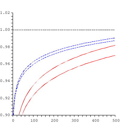
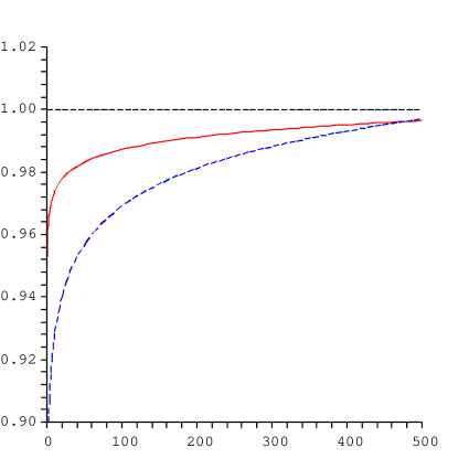
$E~{}(\rm MeV)$                                                                    $E~{}(\rm MeV)$

Figure 1: Examples of the e.m. correction factors for the photon-inclusive widths as a function of the cut on the maximal missing energy. Left: $G_{\pi^{+}\pi^{-}}$ (full lines) and $G_{K^{+}K^{-}}$ (dashed lines) for the corresponding $B$ decays; in each set the two curves are obtained for $\mu=M_{\rho}$ (upper curve) and $\mu=M_{\pi}(M_{K})$ (lower curve). Right: scale-independent ratios $G_{K^{0}\pi^{+}}/G_{K^{+}\pi^{0}}$ (full line) and $G_{\pi^{+}\pi^{-}}/G_{\pi^{+}\pi^{0}}$ (dashed line) for the corresponding $B$ decays.

3 Numerical results and differential distributions

In figure 1 we report a few examples of the e.m. correction factors relevant to $B\to\pi\pi$, $\pi K$, and $KK$ modes. As can be noted, the effects are quite large in case of tight cuts on the photon energy or, equivalently, tight cuts on the invariant mass of the two pseudoscalar mesons. The e.m. effects grow logarithmically with respect to the velocities of the charged particles in the final state and with respect to the cut on the maximal photon energy (relative to the mass of the decaying particle). As a result, the largest effects are found for $B$ decays into charged pions. For instance, the observable ratio $\Gamma[B\to\pi^{+}\pi^{-}(\gamma)]/\Gamma[B\to\pi^{0}\pi^{0}]$, determined with a cut of about 250 MeV on the missing mass of the $\pi^{+}\pi^{-}$ pair, receives a $5\%$ negative isospin-breaking correction with respect to the corresponding theoretical ratio evaluated in absence of soft-photon contributions.

As anticipated, the overall normalization of the $G_{12}(E)$ factors is convention dependent. By construction, they include the whole effect of the bremsstrahlung but only part of the virtual e.m. corrections, namely the leading soft contribution which can be reliably estimated within scalar QED. The separation between hard and soft virtual contributions is arbitrary and determined by the choice of the UV renormalization scale $\mu$. The most natural choice for the latter is between the light pseudoscalar masses ($M_{\pi}$ or $M_{K}$) and $M_{\rho}\approx$ 770 MeV. As shown in the left plot of figure 1, the uncertainty associated with this range is at most of ${\cal O}(1\%)$ and definitely subleading with respect to the leading effects induced by soft contributions.

In principle, this scale uncertainty could be removed by means of an appropriate matching between our effective theory –where photons and mesons are the only dynamical degrees of freedom and each weak amplitude is determined by a momentum-independent coupling– and more predictive effective theories where the weak decay amplitudes are computed in terms of the fundamental SM couplings. In the last few years there has been a substantial progress toward a precise estimate of non-leptonic weak decay amplitudes within the SM (see e.g. Ref. [9] and references therein); however, we are still far from the ${\cal O}(1\%)$ level, especially for the decays into two light pseudoscalar mesons. Moreover, all present approaches do not include the structure-dependent electromagnetic corrections which would allow to match the scale dependence of the $G_{12}(E)$ factors.

Despite the absence of a precise UV matching, in a few cases the e.m. correction factors we have computed allows to evaluate in a precise way the amount of isospin breaking induced by soft photons. As illustrated in the right plot of figure 1, the scale uncertainty drops out completely in all the ratios of two-body photon-inclusive widths with at least one charged particle in the final state.

It is worth to stress that the e.m. corrections discussed in this work can be one of the sources of the “anomalous” isospin-breaking effects identified in recent phenomenological analyses of $B\to\pi K$ and $B\to\pi\pi$ decays [10]. A consistent phenomenological analysis of these channels with the inclusion of radiative corrections requires the information on the experimental cuts applied on the soft-photon radiation and is beyond the purpose of the present work. However, it is clear that radiative corrections need to be included in these channels, especially if one is interested in isospin-breaking effects as a tool to identify possible deviations from the SM.

From the purely experimental side, the only relevant aspect of the $G_{12}(E)$ factors is their energy dependence, which is unambiguously determined up to ${\cal O}(E)$ terms. This allows us to evaluate the observable missing-energy distribution, or the soft-photon spectrum, $d\Gamma^{\rm incl}_{12}(E)/dE$. As is well known, the $E\to 0$ singularity of this distribution is not integrable if evaluated at any fixed order in perturbation theory; however, the all-order resummation of the leading infrared singularities leads to an integrable distribution [1, 2]. In our case, this can be written as

$$\frac{d\Gamma^{\rm incl}_{12}(E)}{dE}~{}=~{}\frac{2\alpha}{\pi}~{}\frac{|b_{12}|\Gamma^{0}_{12}}{E}\left(\frac{2E}{M_{H}}\right)^{\frac{2\alpha}{\pi}|b_{12}|}\left[1+{\cal O}\left(\frac{E}{M_{H}},\frac{\alpha}{\pi}\right)\right]$$ (15)

with the $b_{12}$ coefficients given in eq. (7). The exponentiation of the leading-log corrections does not lead to appreciable numerical difference with respect to the pure ${\cal O}(\alpha)$ result for missing energies above few MeV. However, as discussed in [7], having an integrable distribution can be very useful in preparing a dedicated Montecarlo program.

Concerning the angular distribution of the bremsstrahlung photons, the ${\cal O}(\alpha)$ result reads

$$\frac{d^{2}\Gamma(H\to P_{1}P_{2}\gamma)}{dE_{\gamma}~{}d\cos\theta_{\gamma}}=\frac{\alpha}{2\pi}~{}\frac{\beta_{\gamma}}{\beta}~{}\frac{\Gamma^{0}_{12}}{E_{\gamma}}~{}R_{12}$$ (16)

where $E_{\gamma}$ and $\theta_{\gamma}$ denote, respectively, photon energy and angle between photon and $P_{1}$ momenta in the $H$ meson rest frame, and

$$\beta^{2}~{}=~{}\left[1-\frac{(r_{1}+r_{2})^{2}}{1-2z}\right]\left[1-\frac{(r_{1}-r_{2})^{2}}{1-2z}\right]~{},\qquad z~{}=~{}\frac{E_{\gamma}}{M_{H}}~{}.$$ (17)

The $R_{12}$ coefficients, defined by

$$R_{12}~{}=~{}E_{\gamma}^{2}\sum_{\rm spins}\left|\frac{{\cal A}[H(p_{H})\to P_{1}(p_{1})P_{2}(p_{2})\gamma]}{e{\cal A}(H\to P_{1}P_{2})}\right|^{2}~{}=~{}E_{\gamma}^{2}\left|\sum_{i=H,P1,P2}Q_{i}\frac{p_{i}^{\mu}}{k\cdot p_{i}}\right|^{2}~{},$$ (18)

where $Q_{1,2}$ and $-Q_{H}$ denote, respectively, the electric charges of $P_{1,2}$ and $H$ in units of the electron charge, assume the following explicit form

$$R_{+-} = \frac{1-r_{1}^{2}-r_{2}^{2}-2z}{t_{1}t_{2}}-\frac{r_{1}^{2}}{t_{1}^{2}}-\frac{r_{2}^{2}}{t_{2}^{2}}~{},$$ (19)

$$R_{\pm 0} = \frac{1+r_{1}^{2}-r_{2}^{2}-2z(1-t_{1})}{t_{1}}-\frac{r_{1}^{2}}{t_{1}^{2}}-1~{},$$ (20)

in terms of the kinematical variables

$$t_{1,2}=\frac{1}{2}\left[1+\frac{r_{1,2}^{2}}{1-2z}\mp\beta_{\gamma}\cos\theta_{\gamma}\right]~{}.$$ (21)

4 Conclusions

In the last few years there has been a substantial progress in the experimental determination of two-body non-leptonic $B$ decays into light pseudoscalar mesons. Several new theoretical tools have also been developed for the description of these interesting processes. However, in most cases electromagnetic effects of long-distance origin have been ignored, both in the theoretical predictions and in the experimental analyses. Aiming at accuracies of the order of a few percent, this approximation is no longer valid.

In this work we have presented a detailed discussion of the electromagnetic effects of long-distance origin in two-body non-leptonic $B$ decays. In particular, we have computed the leading ${\cal O}(\alpha)$ effects induced by both real and virtual photons in a generic process of the type $H\to P_{1}P_{2}(\gamma)$, where both $H$ and $P_{1,2}$ are scalar or pseudoscalar particles (with arbitrary masses). The results thus obtained can be applied to both $B$ and $D$ decays.

We have performed the calculation within scalar QED and assuming an effective constant coupling for the weak vertex. Given the universal character of the infrared singularities, this simplified framework allows to identify the leading effects induced by soft photons. The results obtained within this framework are valid up to energy-independent ${\cal O}(\alpha)$ terms related to the matching between this effective theory and the SM, and possible ${\cal O}(E_{\gamma})$ terms associated to the emission of hard photons (which should be identified experimentally). In the case of the photon-inclusive rates, the analytic formulae we have obtained represent a generalization of the results of Ref. [4], which are recovered in the limiting case $M_{1}=M_{2}$. In order to facilitate the experimental simulation of the soft-photon radiation, we have also discussed the corresponding angular and energy distribution.

From the phenomenological point of view, the largest impact of the soft-photon radiation is found in the $B\to\pi^{+}\pi^{-}$ channel, where the corrections to the partially-inclusive rate can easily exceed the $5\%$ level. We stress that detailed estimate of these effects can only be made once the experimental information on the photon cuts (or the missing energy) is available. Without this information, an unambiguous comparison between theory and experiments, and also the combination of different experimental results, cannot be performed.

References

- [1] D. R. Yennie, S. C. Frautschi and H. Suura, Annals Phys. 13 (1961) 379.
- [2] S. Weinberg, Phys. Rev. 140 (1965) B516.
- [3] P. Golonka and Z. Was, hep-ph/0506026.
- [4] V. Cirigliano, J. F. Donoghue and E. Golowich, Eur. Phys. J. C 18 (2000) 83 [hep-ph/0008290]; Phys. Rev. D 61 (2000) 093001, erratum-ibid. D 63 (2001) 059903 [hep-ph/9907341].
- [5] V. Cirigliano et al., Eur. Phys. J. C 23 (2002) 121 [hep-ph/0110153]; ibid. J. C35 (2004) 53 [hep-ph/0401173].
- [6] T. C. Andre, hep-ph/0406006.
- [7] C. Gatti, hep-ph/0507280.
- [8] See e.g. E. Blucher, talk presented at Lepton Photon 2005, Uppsala, Sweden, July 2005.
- [9] M. Beneke, G. Buchalla, M. Neubert and C. T. Sachrajda, Phys. Rev. Lett. 83 (1999) 1914 [hep-ph/9905312]; M. Beneke and M. Neubert, Nucl. Phys. B 675 (2003) 333 [hep-ph/0308039]; Y. Y. Keum, H. N. Li and A. I. Sanda, Phys. Rev. D 63 (2001) 054008 [hep-ph/0004173]; M. Ciuchini, E. Franco, G. Martinelli, M. Pierini and L. Silvestrini, Phys. Lett. B 515 (2001) 33 [hep-ph/0104126], hep-ph/0407073; C. W. Bauer, D. Pirjol, I. Z. Rothstein and I. W. Stewart, Phys. Rev. D 70 (2004) 054015 [hep-ph/0401188].
- [10] See e.g. A. J. Buras, R. Fleischer, S. Recksiegel and F. Schwab, hep-ph/0411373, and references therein.