Confinement and parity doubling in heavy–light mesons

Abstract

In this paper, we study the chiral symmetry restoration in the hadronic spectrum in the framework of generalised Nambu–Jona-Lasinio quark models with instantaneous confining quark kernels. We investigate a heavy–light quarkonium and derive its bound–state equation in the form of a Schrödingerlike equation and, after the exact inverse Foldy–Wouthuysen transformation, in the form of a Diraclike equation. We discuss the Lorentz nature of confinement for such a system and demonstrate explicitly the effective chiral symmetry restoration for highly excited states in the mesonic spectrum. We give an estimate for the scale of this restoration.

I Introduction

Chiral symmetry is spontaneously broken in QCD with light quarks. This immediately implies the existence of light mesons which become Goldstone bosons in the chiral limit, with dynamics described by chiral perturbation theory. Being an effective low–energy reduction of QCD, this theory does not describe the property of confinement.

While the property of colour confinement is expected from general considerations and is supported by lattice calculations, no effective theory exists which derives confinement directly from the QCD Lagrangian, and one is left to rely upon models, such as the constituent quark model, to describe confinement. These models work surprisingly well in the light–quark sector, reproducing the spectrum of low–lying mesonic states, with the exception of ground–state pseudoscalars. So, the conventional wisdom of quark model practitioners is to assume that constituent quarks are indeed the correct degrees of freedom in the non-perturbative domain, with light pseudoscalars being a special case. As there is no hope to obtain Goldstone bosons within any naive quark model which does not address the question of QCD vacuum structure, the sector of light pseudoscalars has to be left outside the scope of the constituent picture.

Phenomenological successes of constituent models are in fact quite remarkable, but there is yet another feature of QCD which they fail to reproduce. Namely, for highly excited hadronic states, we have quark typical momenta much larger than the scale of chiral symmetry breaking so that chiral symmetry should be restored towards the high end of hadronic spectra. The phenomenon signalling this restoration is parity doubling.

Parity doubling has been discussed for many years in connection with the baryon spectrum (see, for example, Glozman ). Quite recently, the observation of the low–mass $D_{s}(2317)$ and $D_{s}(2460)$ mesons D caused a resurgence of interest in the issue of chiral symmetry restoration Eichten ; Nowak . Detailed arguments in favour of parity doubling for higher mesonic states are given in Swanson .

Quite obviously, chiral symmetry restoration is a consequence of fully relativistic dynamics of light quarks and chirally–symmetric quark interaction. Besides, it implies the confining quark interaction, so the models exhibiting parity doubling should interweave confinement and chiral symmetry breaking into one single mechanism. These models do exist in the literature Orsay ; Lisbon , and the possibility of parity doubling in such models was briefly discussed in Orsay2 . These models are introduced in Chapter II and generic mesonic bound–state equations are derived for arbitrary kernels. Chapter III is devoted to the setting up of both the heavy–light bound state equation and its equivalent Diraclike equation. The heavy–light meson can be thought of as a kind of hydrogen atom of soft QCD, with the heavy–quark spin symmetry IW , allowing us to study the dynamics of the light quark ignoring complications related to the full relativistic two–body problem. Then, for arbitrary noncompact (that is, confining) quark kernels, it is shown in Chapter III that these equations necessarily lead to chiral restoration for high momenta. Finally, we end this chapter with a numerical study of the heavy–light mesonic spectrum, using, for the sake of clarity, a simple harmonic oscillator quark kernel (which allows for a differential mass–gap equation) and explicitly show the mechanism of chiral restoration at work. We conclude with Chapter IV.

II Mesonic states in potential quark models

In this section, we briefly give the necessary details of the model to be considered below. The potential quark model, which we call the Nambu–Jone-Lasinio (NJL)-type model after the original paper NJL is given by the Hamiltonian Orsay ; Orsay2 ; Lisbon :

$$\hat{H}=\int d^{3}x\bar{\psi}(\vec{x},t)\left(-i\vec{\gamma}\cdot\vec{\bigtriangledown}+m\right)\psi(\vec{x},t)+\frac{1}{2}\int d^{3}xd^{3}y\;J^{a}_{\mu}(\vec{x},t)K^{ab}_{\mu\nu}(\vec{x}-\vec{y})J^{b}_{\nu}(\vec{y},t),$$ (1)

with the quark currents, $J_{\mu}^{a}(\vec{x},t)=\bar{\psi}(\vec{x},t)\gamma_{\mu}\frac{\lambda^{a}}{2}\psi(\vec{x},t)$, interacting through an instantaneous kernel,

$$K^{ab}_{\mu\nu}(\vec{x}-\vec{y})=g_{\mu 0}g_{\nu 0}\delta^{ab}V_{0}(|\vec{x}-\vec{y}|).$$ (2)

A remarkable feature of the given model is the robustness of the results against variations of the form and parameters of the confining potential $V_{0}({\vec{x}})$. Usually a powerlike form is adopted,

$$V_{0}(|\vec{x}|)=K_{0}^{\alpha+1}|\vec{x}|^{\alpha},$$ (3)

with $0\leqslant\alpha\leqslant 2$. The case of the linearly rising potential $\alpha=1$ (see, for example, linear ; Simonov1 ) is strongly supported by hadronic phenomenology, whereas the marginal case of $\alpha=2$ — the harmonic oscillator potential — leads to simpler, differential, equations and is considered by many authors Orsay ; Orsay2 ; Lisbon ; pnea because, despite of its mathematical simplicity, it already yields a physical picture for the mechanism of dynamical chiral symmetry breaking not unlike the one given by linear confinement.

The quark models of this class fulfill the well-known low energy theorems of Gell-Mann, Oakes, and Renner GOR , Goldberger and Treiman GT , Adler selfconsistency zero ASC , the Weinberg theorem Wein , and so on. For an early derivation of the Gell-Mann–Oakes–Renner relation, for this class of models, see Ref. Orsay2 . For the derivation of the Weinberg theorem see Ref. EmilCota . The Salpeter equations for these models can be seen in detail in Ref. Lisbon . Using this formalism it is possible to give, for the class of models embodied in Eq. (1), an analytic proof of the Goldberger–Treiman relation BicudAp . The same formalism can be used to give an analytic proof of all the above low-energy theorems. The axial anomaly and the $\pi\gamma\gamma$ coupling constant can be derived naturally in the framework of the given model as well, following, for example, the lines of the textbook CL and using the asymptotic freedom and the Ward identity for the dressed axial vertex BicudAp (see also Ref. pi2g for an independent derivation of this relation in the Dyson–Schwinger approach to the dressed quark propagator).

The standard approach — valid for any $\alpha$ — to the model (1) is the Bogoliubov transformation from bare to dressed quarks, parametrised through the chiral angle $\varphi_{p}$:

$$\psi_{\beta}(\vec{x},t)=\sum_{s=\uparrow,\downarrow}\int\frac{d^{3}p}{(2\pi)^{3}}e^{i\vec{p}\vec{x}}[\hat{b}_{\beta s}(\vec{p},t)u_{s}(\vec{p})+\hat{d}_{\beta s}^{\dagger}(-\vec{p},t)v_{s}(-\vec{p})],$$ (4)

$$\left\{\begin{array}[]{rcl}u(\vec{p})&=&\frac{1}{\sqrt{2}}\left[\sqrt{1+\sin\varphi_{p}}+\sqrt{1-\sin\varphi_{p}}\;(\vec{\alpha}\hat{\vec{p}})\right]u(0),\\ v(-\vec{p})&=&\frac{1}{\sqrt{2}}\left[\sqrt{1+\sin\varphi_{p}}-\sqrt{1-\sin\varphi_{p}}\;(\vec{\alpha}\hat{\vec{p}})\right]v(0),\end{array}\right.$$ (5)

where $E_{p}$ stands for the dispersive law of the dressed quarks; $\beta$ being the colour index, $\beta=\overline{1,N_{C}}$. In what follows the limit $N_{C}\gg 1$ is assumed. It is convenient to define the chiral angle varying in the range $-\frac{\pi}{2}<\varphi_{p}\leqslant\frac{\pi}{2}$, with the boundary conditions $\varphi(0)=\frac{\pi}{2}$, $\varphi(p\to\infty)\to 0$.

The Hamiltonian (1) normal ordered in the basis (4) can be split into three parts,

$$\hat{H}=E_{\rm vac}+:\hat{H}_{2}:+:\hat{H}_{4}:,$$ (6)

the first part being the vacuum energy, and the second and the third parts being quadratic and quartic in terms of single–quark operators. The requirement that $:\hat{H}_{2}:$ should be diagonal — the anomalous Bogoliubov term be absent — leads one to the mass–gap equation for the chiral angle,

$$A_{p}\cos\varphi_{p}-B_{p}\sin\varphi_{p}=0,$$ (7)

with

$$A_{p}=m+\frac{1}{2}\int\frac{d^{3}k}{(2\pi)^{3}}V(\vec{p}-\vec{k})\sin\varphi_{k},\quad B_{p}=p+\frac{1}{2}\int\frac{d^{3}k}{(2\pi)^{3}}\;(\hat{\vec{p}}\hat{\vec{k}})V(\vec{p}-\vec{k})\cos\varphi_{k}.$$ (8)

We absorb the fundamental Casimir operator $C_{F}$ into the definition of the potential, $V(\vec{p}-\vec{k})=C_{F}V_{0}(\vec{p}-\vec{k})$ by rescaling the parameter $K_{0}$.

For the chiral angle — solution to the mass–gap equation (7) — the Hamiltonian (6) takes the form:

$$\hat{H}=E_{\rm vac}+\sum_{\beta}\sum_{s=\uparrow,\downarrow}\int\frac{d^{3}p}{(2\pi)^{3}}E_{p}[\hat{b}^{\dagger}_{\beta s}(\vec{p})\hat{b}_{\beta s}(\vec{p})+\hat{d}^{\dagger}_{\beta s}(-\vec{p})\hat{d}_{\beta s}(-\vec{p})]+O\left(\frac{1}{\sqrt{N_{C}}}\right),$$ (9)

with the corrections coming from the $:\hat{H}_{4}:$ part. This completes diagonalisation of the Hamiltonian (1) in the single–particle sector of the theory (the so-called BCS level BCS ). The dressed–quark dispersive law can be built as

$$E_{p}=A_{p}\sin\varphi_{p}+B_{p}\cos\varphi_{p}.$$ (10)

It was found in Ref. 2d that the ’t Hooft model for two–dimensional QCD tHooft in the axial gauge, which is identical to the model (1) in two dimensions BG , admits a further diagonalisation in terms of colourless mesonic states, which is a step beyond the BCS approximation. This method was generalised, in Ref. nr , to the class of NJL-type four–dimensional models (1). The key idea was to rewrite the Hamiltonian (6), in the centre–of–mass frame,

$$\hat{H}=E_{\rm vac}^{\prime}+\int\frac{d^{3}P}{(2\pi)^{3}}\hat{\cal H}(\vec{P}),\quad\hat{\cal H}(0)\equiv\hat{\cal H},$$

in terms of compound quark–antiquark operators,

$$\hat{M}_{ss^{\prime}}(\vec{p},\vec{p}^{\prime})=\frac{\displaystyle 1}{\displaystyle\sqrt{N_{C}}}\sum_{\beta}\hat{d}_{\beta s}(-\vec{p})\hat{b}_{\beta s^{\prime}}(\vec{p}^{\prime}),$$ (11)

and to perform a second, generalised, Bogoliubov transformation, “dressing” the bare operators (11) with the coherent cloud of quark–antiquark pairs. The operators creating/annihilating the physical mesonic states in the theory are given by

$$\left\{\begin{array}[]{l}\hat{m}_{n\nu}=\displaystyle\int\frac{p^{2}dp}{(2\pi)^{3}}\left[\hat{M}_{\nu}(p)\varphi_{n\nu}^{+}(p)-\hat{M}^{\dagger}_{\nu}(p)\varphi_{n\nu}^{-}(p)\right]\\ \hat{m}_{n\nu}^{\dagger}=\displaystyle\int\frac{p^{2}dp}{(2\pi)^{3}}\left[\hat{M}_{\nu}^{\dagger}(p)\varphi_{n\nu}^{+}(p)-\hat{M}_{\nu}(p)\varphi_{n\nu}^{-}(p)\right],\end{array}\right.$$ (12)

where the operators (11) are expanded first,

$$\hat{M}_{ss^{\prime}}(\vec{p},\vec{p})=\sum_{\nu}[\kappa_{\nu}(\hat{\vec{p}})]_{ss^{\prime}}\hat{M}_{\nu}(p),$$ (13)

using an appropriate basis diagonalising the spin–angular structure of the Hamiltonian. Such a basis is known to be formed by the $\{nJ^{PC}\}$ states ($n$ being the radial quantum number), for which we use the shorthand notation $\{n\nu\}$. The centre–of–mass Hamiltonian $\hat{\cal H}$ takes a diagonal form,

$$\hat{\cal H}=\sum_{n,\nu}M_{n\nu}m^{\dagger}_{n\nu}m_{n\nu}+O\left(\frac{1}{\sqrt{N_{C}}}\right),$$ (14)

provided the mesonic wave functions obey the bound–state equation,

$$\left\{\begin{array}[]{l}[2E_{p}-M_{n\nu}]\varphi_{n\nu}^{+}(p)=\displaystyle\int\frac{\displaystyle k^{2}dk}{\displaystyle(2\pi)^{3}}[T^{++}_{\nu}(p,k)\varphi_{n\nu}^{+}(k)+T^{+-}_{\nu}(p,k)\varphi_{n\nu}^{-}(k)]\\[0.0pt] [2E_{p}+M_{n\nu}]\varphi_{n\nu}^{-}(p)=\displaystyle\int\frac{\displaystyle k^{2}dk}{\displaystyle(2\pi)^{3}}[T^{-+}_{\nu}(p,k)\varphi_{n\nu}^{+}(k)+T^{--}_{\nu}(p,k)\varphi_{n\nu}^{-}(k)],\end{array}\right.$$ (15)

with the orthonormality conditions

$$\begin{array}[]{l}\displaystyle\int\frac{p^{2}dp}{(2\pi)^{3}}\left[\varphi_{n\nu}^{+}(p)\varphi_{m\nu}^{+}(p)-\varphi_{n\nu}^{-}(p)\varphi_{m\nu}^{-}(p)\right]=\delta_{nm},\\[8.53581pt] \displaystyle\int\frac{p^{2}dp}{(2\pi)^{3}}\left[\varphi_{m\nu}^{+}(p)\varphi_{n\nu}^{-}(p)-\varphi_{m\nu}^{-}(p)\varphi_{n\nu}^{+}(p)\right]=0,\end{array}$$ (16)

which follow directly from the canonical bosonic commutation relations of the operators (12). This completes the diagonalisation of the theory (1), in terms of the physical observable degrees of freedom. The bound–state Eq. (15) can be derived alternatively from the Bethe–Salpeter equation for mesonic states Orsay ; Orsay2 ; Lisbon ; Lisbon2 . We resort to this method below. The eigenvalue problem (15) is subject to numerical investigation (see Ref. Orsay and also Ref. Lisbon2 where, in particular, the evolution of the vector–pseudoscalar mass splitting as a function of the current quark mass is studied in detail), and no problem is met when building the mesonic spectrum for the whole class of theories (1).

III A Heavy–light system

III.1 The bound–state equation

An important feature of the bound–state Eq. (15) is the fact that each mesonic state is described by means of a two–component wave function, $\varphi_{n\nu}^{\pm}(p)$. The physical meaning of these two components is obvious: $\varphi_{n\nu}^{+}(p)$ describes the forward motion, in time, of the mesonic quark–antiquark pair and $\varphi_{n\nu}^{-}(p)$ its time backward motion. Strictly speaking, for a given set of quantum numbers, four eigenfunctions should be considered — two for the eigenvalue $M_{n\nu}$ and two for $-M_{n\nu}$. Meanwhile, the bound–state Eq. (15) supports the symmetry

$$\{M_{n\nu},\varphi_{n\nu}^{\pm}(p)\}\leftrightarrow\{-M_{n\nu},\varphi_{n\nu}^{\mp}(p)\},$$ (17)

that can be easily verified using its explicit form. Due to the instantaneous interaction, both particles in the meson move forward and backward in time in unison. This leads us to an immediate conclusion that the heavy–light meson, with the static–quark Zitterbewegung suppressed by its infinite mass, can be described with a one–component wave function, so that

$$\varphi_{n\nu}^{+}(p)\equiv\varphi_{n\nu}(p),\quad\varphi_{n\nu}^{-}(p)=0,$$ (18)

and the bound–state equation can be considerably simplified in this case. Although Eq. (15) is written for the single–flavour theory, its generalisation for two flavours is trivial yielding for the heavy–light bound–state equation:

$$[m_{\bar{Q}}+E_{p}-M_{n\nu}]\varphi_{n\nu}(p)=\displaystyle\int\frac{\displaystyle k^{2}dk}{\displaystyle(2\pi)^{3}}T^{++}_{\nu}(p,k)\varphi_{n\nu}(k),$$ (19)

with $m_{\bar{Q}}$ being the static–antiquark mass. The amplitude $T^{++}_{\nu}(p,k)$ can be built using the Hamiltonian approach described in the previous section, though we find it more instructive to derive the heavy–light bound–state Eq. (19) using an alternative approach, employing the Bethe–Salpeter equation. To this end, we start from the homogeneous Bethe–Salpeter equation for the mesonic Salpeter amplitude $\chi({\vec{p}};M)$,

$$\chi({\vec{p}};M)=-i\int\frac{d^{4}k}{(2\pi)^{4}}V(\vec{p}-\vec{k})\;\gamma_{0}S_{q}({\vec{k}},k_{0}+M/2)\chi({\vec{k}};M)S_{\bar{Q}}({\vec{k}},k_{0}-M/2)\gamma_{0},$$ (20)

where

$$S_{q}({\vec{p}},p_{0})=\frac{\Lambda^{+}({\vec{p}})\gamma_{0}}{p_{0}-E_{p}+i\epsilon}+\frac{{\Lambda^{-}}({\vec{p}})\gamma_{0}}{p_{0}+E_{p}-i\epsilon}$$ (21)

is the dressed light–quark propagator. The projectors are defined as

$$\Lambda^{\pm}(\vec{p})=T_{p}P_{\pm}T_{p}^{\dagger},\quad P_{\pm}=\frac{1\pm\gamma_{0}}{2},\quad T_{p}=\exp{\left[-\frac{1}{2}(\vec{\gamma}\hat{\vec{p}})\left(\frac{\pi}{2}-\varphi_{p}\right)\right]}.$$ (22)

Since, for the static particle, the chiral angle is simply $\varphi_{\bar{Q}}(p)=\frac{\pi}{2}$, then the dispersive law and the projectors become trivial, giving for the heavy–quark propagator:

$$S_{\bar{Q}}({\vec{p}},p_{0})=\frac{P_{+}\gamma_{0}}{p_{0}-m_{\bar{Q}}+i\epsilon}+\frac{P_{-}\gamma_{0}}{p_{0}+m_{\bar{Q}}-i\epsilon}.$$ (23)

It is convenient to define a modified vertex,

$$\tilde{\varGamma}(\vec{p})=\int\frac{dp_{0}}{2\pi}S_{q}(\vec{p},p_{0}+M/2)\chi(\vec{p};M)S_{\bar{Q}}(\vec{p},p_{0}-M/2),$$ (24)

and to perform its Foldy–Wouthuysen transformation by means of the operator $T_{p}^{\dagger}$,

$$\varGamma(\vec{p})=T_{p}^{\dagger}\tilde{\varGamma}(\vec{p})\hat{1},$$ (25)

where, for the sake of transparency, we kept the unity on the r.h.s. for the operator rotating the static antiquark. The resulting matrix bound–state equation reads:

$$(E-E_{p})\varGamma(\vec{p})=P_{+}\left[\int\frac{d^{3}k}{(2\pi)^{3}}V(\vec{p}-\vec{k})T_{p}^{\dagger}T_{k}\varGamma(\vec{k})\right]P_{-},$$ (26)

where we defined the energy excess over the static–particle mass, $E=M-m_{\bar{Q}}$. The form of the r.h.s. of Eq. (26) suggests that the matrix $\varGamma(\vec{p})$ should have the structure

$$\varGamma(\vec{p})=\left(\begin{array}[]{cc}0&\psi(\vec{p})\\ 0&0\end{array}\right)={\psi(\vec{p})\choose 0}_{q}\otimes(0\;1)_{\bar{Q}},$$ (27)

where, for future convenience, we split the matrix into the direct product of the light– and heavy–particle components. Then the eigenstate equation for the wave function $\psi(\vec{p})$ can be derived in the form of a Schrödingerlike equation,

$$E_{p}\psi(\vec{p})+\int\frac{d^{3}k}{(2\pi)^{3}}V({\vec{p}}-{\vec{k}})\left[C_{p}C_{k}+({\vec{\sigma}}\hat{{\vec{p}}})({\vec{\sigma}}\hat{{\vec{k}}})S_{p}S_{k}\right]\psi(\vec{k})=E\psi(\vec{p}),$$ (28)

with

$$C_{p}=\cos\frac{1}{2}\left(\frac{\pi}{2}-\varphi_{p}\right),\quad S_{p}=\sin\frac{1}{2}\left(\frac{\pi}{2}-\varphi_{p}\right).$$ (29)

The heavy–light bound–state Eq. (28) is the main object for studies in the present paper. However, it is instructive to rewrite it in the Diraclike form, which allows one to investigate the Lorentz nature of confinement in the heavy–light quarkonium. First, notice that Eq. (26) is written for the positive–energy solutions, $M=m_{\bar{Q}}+E>0$. Similarly, for the negative–energy solutions, $M=-m_{\bar{Q}}-E<0$, although the same Schrödingerlike Eq. (28) holds, but the matrix $\varGamma(\vec{p})$ takes a different form,

$$\varGamma(\vec{p})=\left(\begin{array}[]{cc}0&0\\ \psi(\vec{p})&0\end{array}\right)={0\choose\psi(\vec{p})}_{\bar{q}}\otimes(1\;0)_{Q},$$ (30)

which can be easily guessed from the symmetry (17) and the specific property of the heavy–light system (18). Thus the Foldy–rotated wave functions of the light component of the system, responsible for the positive– and negative–energy solutions, can be written, according to Eqs. (27), (30), as

$$\Psi(\vec{p})={\psi(\vec{p})\choose 0},$$

for positive energies and as

$$\Psi(\vec{p})={0\choose\psi(\vec{p})},$$

for negative energies. In view of the passive role played by the static particle, we shall refer to $\Psi(\vec{p})$ as to the wave function of the entire heavy–light system. Consequently, the bound–state Eq. (28) can be rewritten for $\Psi(\vec{p})$,

$$E_{p}\Psi(\vec{p})+\frac{1}{2}\int\frac{d^{3}k}{(2\pi)^{3}}V({\vec{p}}-{\vec{k}})\left[T_{p}T_{k}^{\dagger}+T_{p}^{\dagger}T_{k}\right]\Psi(\vec{k})=\gamma_{0}E\Psi(\vec{k}).$$ (31)

As it follows immediately from Eq. (25), the Foldy operator which splits the positive– and negative–energy components of this wave function is $T_{p}^{\dagger}$: $\Psi(\vec{p})=T_{p}^{\dagger}\tilde{\Psi}(\vec{p})$. Therefore, the pre–Foldy bound–state equation for the wave function $\tilde{\Psi}(\vec{p})$ follows from Eq. (31) after the counter–rotation with the operator $T_{p}$,

$$E_{p}U_{p}\tilde{\Psi}({\vec{p}})+\frac{1}{2}\int\frac{d^{3}k}{(2\pi)^{3}}V({\vec{p}}-{\vec{k}})(U_{p}+U_{k})\tilde{\Psi}({\vec{k}})=E\tilde{\Psi}({\vec{p}}),$$ (32)

where, for future convenience, we introduced the unitary operator

$$U_{p}=T_{p}\gamma_{0}T_{p}^{\dagger}=\gamma_{0}\sin\varphi_{p}+({\vec{\alpha}}\hat{{\vec{p}}})\cos\varphi_{p}.$$ (33)

Then, using the mass–gap Eq. (7), rewritten in the form:

$$E_{p}U_{p}={\vec{\alpha}}{\vec{p}}+\beta m+\frac{1}{2}\int\frac{d^{3}k}{(2\pi)^{3}}V({\vec{p}}-{\vec{k}})U_{k},$$ (34)

we arrive at the heavy–light bound–state equation in the form of a Diraclike equation for the light quark, in coordinate space,

$$({\vec{\alpha}}{\vec{p}}+\beta m)\tilde{\Psi}({\vec{x}})+\int d^{3}z\Lambda({\vec{x}},{\vec{z}})K({\vec{x}},{\vec{z}})\tilde{\Psi}({\vec{z}})=E\tilde{\Psi}({\vec{x}}),$$ (35)

with

$$K({\vec{x}},{\vec{z}})=\frac{1}{2}[V({\vec{x}})+V({\vec{z}})-V({\vec{x}}-{\vec{z}})]$$ (36)

and

$$\Lambda({\vec{p}},{\vec{q}})=(2\pi)^{3}\delta^{(3)}({\vec{p}}-{\vec{q}})U_{p}.$$ (37)

Notice that the matrix $\Lambda({\vec{p}},{\vec{k}})$ Simonov1 can be related to the Green’s function as

$$\Lambda({\vec{p}},{\vec{k}})=2i\int\frac{d\omega}{2\pi}S(\omega,{\vec{p}},{\vec{k}})\gamma_{0},$$ (38)

where we can use either the dressed light–quark propagator $S_{q}$, defined in Eq. (21),

$$S(\omega,{\vec{p}},{\vec{k}})=(2\pi)^{3}\delta^{(3)}({\vec{p}}-{\vec{k}})S_{q}({\vec{p}},\omega),$$

or the entire heavy–light Green’s function, built using the standard spectral decomposition, with the help of the solutions of the eigenstate problem (35),

$$S(\omega,{\vec{p}},{\vec{k}})=\sum_{E_{n}>0}\frac{\tilde{\Psi}_{n}({\vec{p}})\tilde{\Psi}^{\dagger}_{n}({\vec{k}})\gamma_{0}}{\omega-E_{n}+i0}+\sum_{E_{n}<0}\frac{\tilde{\Psi}_{n}({\vec{p}})\tilde{\Psi}^{\dagger}_{n}({\vec{k}})\gamma_{0}}{\omega+E_{n}-i0}.$$

This feature should not come as a surprise since, as mentioned before, the static antiquark decouples from the system, providing the overall colour neutrality of the bound state.

The Lorentz nature of confinement in the effective one–particle Eq. (35) follows from the matrix structure of $\Lambda({\vec{p}},{\vec{k}})$ Simonov1 , or equivalently, of $U_{p}$ for the given values of the relative momentum $p$ involved. Below, we consider in detail the three regimes which can be identified in the spectrum of hadrons. Although the heavy–light system was used before to arrive at the quark–antiquark bound–state equation, all qualitative conclusions obviously hold for an arbitrary hadronic system.

For small relative momenta the chiral regime takes place. Chiral symmetry breaking — spontaneous or explicit — plays a dominating role, the chiral angle being close to $\frac{\pi}{2}$. As a result, $U_{p}\approx\gamma_{0}$ and the effective interquark interaction becomes purely scalar (even in the absence of any microscopic scalar force). For light quarks, the dressed–quark dispersive law $E_{p}$ differs drastically from the free–particle form of $\sqrt{{\vec{p}}^{2}+m^{2}}$, it may even become negative at small momenta — a necessary feature to have the light (massless) chiral pion. This chiral regime — where the effective interaction is purely scalar — holds below some effective dynamically generated low–energy scale, which we call the BCS scale $\Lambda_{\rm BCS}$, that is, holds for the mean relative interquark momentum $p\lesssim\Lambda_{\rm BCS}$. The BCS scale gives a measure of chiral symmetry breaking in the low–energy domain of the theory and it is closely related to the scale of confinement or, equivalently, to $\Lambda_{\rm QCD}$: $\Lambda_{\rm BCS}\simeq\Lambda_{\rm QCD}$. As soon as the mass of the quark–antiquark state grows, as does the mean relative interquark momentum, the vectorial part of the interquark interaction becomes more important. Finally, the chiral angle becomes negligibly small and the interaction acquires a purely vectorial nature. Thus, we arrive at the chiral symmetry restoration in the spectrum discussed in the literature Swanson ; Glozman ; Nowak .

Note, in passing, that the Dirac structure of the matrix $\Lambda({\vec{p}},{\vec{k}})$ is saturated by the scalar and space–vectorial part, so there is no room for the time–vectorial interaction, dangerous from the point of view of the Klein paradox.

III.2 Chiral symmetry restoration in the spectrum

III.2.1 General remarks

It is argued in the literature Orsay2 ; Swanson ; Nowak ; Glozman that, for highly excited states in the hadronic spectrum, the chiral symmetry should be restored and the states with opposite parity should come in doublets. This statement can be proved using the properties of the bound–state Eq. (28). Indeed, let $\psi(\vec{p})$ be a solution to Eq. (28) with the eigenvalue $E$. Consider

$$\psi^{\prime}(\vec{p})=({\vec{\sigma}}\hat{{\vec{p}}})\psi(\vec{p}),$$ (39)

which, by construction, possesses an opposite parity to $\psi(\vec{p})$. The eigenvalue problem for the new wave function $\psi^{\prime}(\vec{p})$ can be easily derived by multiplying Eq. (28) by $({\vec{\sigma}}\hat{{\vec{p}}})$ from the left,

$$E_{p}\psi^{\prime}(\vec{p})+\int\frac{d^{3}k}{(2\pi)^{3}}V({\vec{p}}-{\vec{k}})\left[S_{p}S_{k}+({\vec{\sigma}}\hat{{\vec{p}}})({\vec{\sigma}}\hat{{\vec{k}}})C_{p}C_{k}\right]\psi^{\prime}(\vec{k})=E\psi^{\prime}(\vec{p}),$$ (40)

where $C_{p}$ and $S_{p}$ are interchanged as compared to Eq. (28). Notice that, for large momenta, one arrives at the relation $C_{p}=S_{p}=\frac{1}{\sqrt{2}}$, which follows directly from the definition of the functions $C_{p}$ and $S_{p}$ (29) and the large–momentum behaviour of the chiral angle, $\varphi_{p}\mathop{\to}\limits_{p\to\infty}0$ (see the first plot at Fig. 1). Therefore, for highly excited states, which possess a large relative interquark momentum, the bound–state Eqs. (28) and (40) coincide, being simply

$$E_{p}\psi(\vec{p})+\frac{1}{2}\int\frac{d^{3}k}{(2\pi)^{3}}V({\vec{p}}-{\vec{k}})\left[1+({\vec{\sigma}}\hat{{\vec{p}}})({\vec{\sigma}}\hat{{\vec{k}}})\right]\psi(\vec{k})=E\psi(\vec{p}),$$ (41)

so that the states $\psi(\vec{p})$ and $({\vec{\sigma}}\hat{{\vec{p}}})\psi(\vec{p})$ become degenerate. Thus, in the framework of the potential quark model (1), one can investigate the explicit mechanism of the chiral symmetry restoration high in the hadronic spectrum. For further convenience, in addition to the BCS scale $\Lambda_{\rm BCS}$ defined above, which can be related, for example, to the chiral condensate,

$$\langle\bar{q}q\rangle=-\frac{3}{\pi^{2}}\int_{0}^{\infty}dp\;p^{2}\sin\varphi_{p}\equiv-(\Lambda_{\rm BCS})^{3},$$ (42)

we introduce the scale of the symmetry restoration $\Lambda_{\rm rest}$, to be defined as the scale at which the splitting within the chiral doublet is much smaller than the BCS scale $\Lambda_{\rm BCS}$. Such a definition is natural since, alternatively, the BCS scale can be defined as the splitting within a chiral doublet at small values of the relative interquark momentum, that is, in the region where this splitting is essentially dictated by chiral symmetry. The numerical estimate for $\Lambda_{\rm rest}$ in the case of the harmonic confinement ($\alpha=2$) is given below.

     

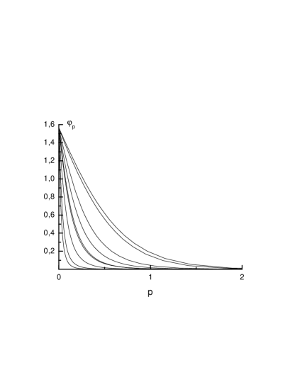
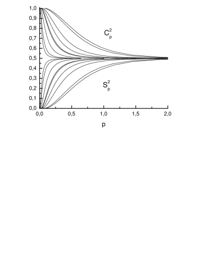
Figure 1: Solutions to the mass–gap Eq. (7) (the first plot) and the coefficients $C_{p}^{2}$ and $S_{p}^{2}$ (the second plot) for the potential $V(r)=K_{0}^{\alpha+1}r^{\alpha}$ with various $\alpha$’s. We plot the curves for $\alpha=0.3$, 0.5, 0.7, 0.9, 1.0, 1.1, 1.3, 1.7, and 2.0 (smaller $\alpha$’s correspond to steeper curves at the origin). The momentum $p$ is given in units of $K_{0}$.

For large interquark momenta, the functions $C_{p}$ and $S_{p}$ are smooth and slow, remaining almost constant when approaching their large-$p$ asymptote of $\frac{1}{\sqrt{2}}$. Therefore, since, for confining potentials, the distribution given by the Fourier transform $V({\vec{p}}-{\vec{k}})$ has the support at ${\vec{k}}\approx{\vec{p}}$, it is possible to consider, approximately, $C_{p}C_{k}\approx C_{p}^{2}$, $S_{p}S_{k}\approx S_{p}^{2}$ and to study $C_{p}^{2}$ and $S_{p}^{2}$ (see the second plot at Fig. 1). This approximation can be easily checked for the harmonic oscillator potential, for which $V({\vec{p}}-{\vec{k}})\propto\Delta_{k}\delta^{(3)}({\vec{p}}-{\vec{k}})$. Taking the corresponding integral by parts, one can omit, for large momenta, the terms containing derivatives of the almost constant functions $C_{k}$ and $S_{k}$. Thus, the chiral symmetry is restored as soon as the difference $C_{p}^{2}-S_{p}^{2}$ becomes negligible. Using the definition (29), one can find that $C_{p}^{2}-S_{p}^{2}=\sin\varphi_{p}=\varphi_{\pi}^{\pm}(p)$, with $\varphi_{\pi}^{\pm}(p)$ being the wave function of the chiral pion, with coinciding positive– and negative–energy components Orsay ; Orsay2 ; Lisbon . Therefore, we conclude that chiral symmetry is restored in the spectrum if the pionic wave function vanishes for the given values of the relative interquark momentum. This gives us an explicit physically transparent relation between the BCS scale and the scale of the symmetry restoration. Although, formally, both scales $\Lambda_{\rm rest}$ and $\Lambda_{\rm BCS}$ are defined by the only dimensional parameter in the theory $K_{0}$, we expect, due to numerical factors, the relation $\Lambda_{\rm rest}\gg\Lambda_{\rm BCS}$ to hold. Below, we perform a numerical check of this relation and estimate the value of the restoration scale.

III.2.2 Numerical estimates: Harmonic oscillator potential

In this paragraph and in order to illustrate the general results obtained so far, we perform an explicit numerical study of the heavy–light mesonic spectrum. To avoid unnecessary complications, we consider the case of the harmonic oscillator potential, which allows us to formulate the mass–gap equation and the bound–state problem through differential equations. This corresponds to the case $\alpha=2$ for the potential (3). Then the Fourier transform of the potential is the Laplacian of the three–dimensional delta–function,

$$V({\vec{p}}-{\vec{k}})=-K_{0}^{3}\Delta_{k}\delta^{(3)}({\vec{p}}-{\vec{k}}),$$ (43)

the chiral angle is the solution to the differential mass–gap equation,

$$p^{3}\sin\varphi_{p}=\frac{1}{2}K_{0}^{3}\left[p^{2}\varphi^{\prime\prime}_{p}+2p\varphi_{p}^{\prime}+\sin 2\varphi_{p}\right]+mp^{2}\cos\varphi_{p},$$ (44)

and the dressed quark dispersive law can be calculated as

$$E_{p}=m\sin\varphi_{p}+p\cos\varphi_{p}-K_{0}^{3}\left[\frac{(\varphi^{\prime}_{p})^{2}}{2}+\frac{\cos^{2}\varphi_{p}}{p^{2}}\right].$$ (45)

In order to introduce the BCS scale we, following the approach suggested before, evaluate the chiral condensate,

$$\langle\bar{q}q\rangle=-\frac{3}{\pi^{2}}\int_{0}^{\infty}dp\;p^{2}\sin\varphi_{p}\approx-(0.51K_{0})^{3}\equiv-(\Lambda_{\rm BCS})^{3},$$ (46)

which gives us

$$K_{0}=490MeV,$$ (47)

if the standard value of the chiral condensate of $-(250MeV)^{3}$ is used in order to fix $\Lambda_{\rm BCS}$. Following the definition of the symmetry restoration formulated above, we demand that the mass splitting in a chiral doublet $\Delta E$ should be much less than $\Lambda_{\rm BCS}$, being, at most, just a few per cent of $250MeV$.

In order to solve the bound–state Eq. (28), we use, as a conventional scheme for the quantum numbers $\nu$, the angular momentum $l$ and the total momentum $j=l\pm\frac{1}{2}$ of the light quark, so that the wave function $\psi({\vec{p}})$ can be expanded as

$$\psi({\vec{p}})=\Omega_{jlm}(\hat{\vec{p}})\frac{u(p)}{p},$$ (48)

with $u(p)$ being the radial wave function, and the spherical spinors are defined as

$$\Omega_{jlm}(\hat{\vec{p}})=\sum_{\mu_{1}\mu_{1}}C^{jm}_{l\mu_{1}\frac{1}{2}\mu_{2}}Y_{l\mu_{1}}(\hat{\vec{p}})\chi_{\mu_{2}}.$$ (49)

Then, the eigenvalue equation for the radial wave function $u(p)$ can be readily derived from the bound–state Eq. (28) in the form:

$$u^{\prime\prime}=[E_{p}-E]u+K_{0}^{3}\left[\frac{(\varphi_{p}^{\prime})^{2}}{4}+\frac{(j+1/2)^{2}}{p^{2}}+\frac{\kappa}{p^{2}}\sin\varphi_{p}\right]u,$$ (50)

where

$$\kappa=\left\{\begin{array}[]{ccc}l,&{\rm for}&j=l-\frac{1}{2}\\ -(l+1),&{\rm for}&j=l+\frac{1}{2}\end{array}=\pm\left(j+\frac{1}{2}\right).\right.$$

Notice that Eq. (50) can be rewritten in the form of a Schrödigerlike equation,

$$-K_{0}^{3}u^{\prime\prime}+V_{[j,l]}(p)u=Eu,$$ (51)

with the effective potential

$$V_{[j,l]}(p)=E_{p}+K_{0}^{3}\left[\frac{1}{4}\varphi_{p}^{\prime 2}+\frac{(j+1/2)^{2}}{p^{2}}+\frac{\kappa}{p^{2}}\sin\varphi_{p}\right].$$ (52)

The well–known property of the spherical spinors,

$$({\vec{\sigma}}\hat{{\vec{p}}})\Omega_{jlm}(\hat{\vec{p}})=-\Omega_{jl^{\prime}m}(\hat{\vec{p}}),\quad l+l^{\prime}=2j,$$ (53)

ensures that the states with $j=l\pm\frac{1}{2}$ possess opposite parity. The splitting between such states is the subject of our investigation, and it follows immediately from Eq. (52) that, for the given total momentum $j$, this splitting is due to the $\kappa$–dependent term in this effective potential. Thus, for $\kappa=\pm(j+\frac{1}{2})$, one finds for the difference of the opposite–parity potentials:

$$\Delta V=-\frac{(2j+1)K_{0}^{3}}{p^{2}}\sin\varphi_{p},$$ (54)

which gives us an explicit example of the relation between the pionic wave function $\sin\varphi_{p}$ and the opposite–parity state splitting, discussed above in general terms.

Table 1: The masses of orbitally excited states and the splittings for the radial quantum number $n=0$, as solutions to the bound–state Eq. (51) with the potential (52). The solutions of the Salpeter Eq. (55) are also listed for the sake of comparison. All energies are given in units of $K_{0}$.

$j$	1/2	3/2	5/2	7/2
$E_{l=j-\frac{1}{2}}$	2.04	3.51	4.51	5.35
$E_{l=j+\frac{1}{2}}$	2.66	3.69	4.57	5.36
$\Delta E_{j}$	0.62	0.18	0.06	0.01
$E_{l=j-\frac{1}{2}}^{\rm Salp}$	2.34	3.36	4.24	5.05
$E_{l=j+\frac{1}{2}}^{\rm Salp}$	3.36	4.24	5.05	5.79
$\Delta E_{j}^{\rm Salp}$	1.02	0.88	0.81	0.74

Table 2: The masses of orbitally excited states and the splittings for the radial quantum number $n=1$, as solutions to the bound–state Eq. (51) with the potential (52). The solutions of the Salpeter Eq. (55) are also listed for the sake of comparison. All energies are given in units of $K_{0}$.

$j$	1/2	3/2	5/2	7/2
$E_{l=j-\frac{1}{2}}$	3.91	5.03	5.87	6.60
$E_{l=j+\frac{1}{2}}$	4.39	5.17	5.92	6.61
$\Delta E_{j}$	0.48	0.14	0.05	0.01
$E_{l=j-\frac{1}{2}}^{\rm Salp}$	4.09	4.88	5.63	6.33
$E_{l=j+\frac{1}{2}}^{\rm Salp}$	4.88	5.63	6.33	7.00
$\Delta E_{j}^{\rm Salp}$	0.79	0.75	0.70	0.67

It is clear from Eq. (54) and from the form of the chiral angle (the first plot at Fig. 1) that the splitting vanishes for excited states, since the excited wave function is localised at larger relative momenta, whereas the chiral angle decreases fast with $p$. In order to prove this property explicitly, we solve the bound–state Eq. (50) numerically. The results are listed in Tables I,II. They demonstrate a clear pattern of chiral symmetry restoration for orbitally excited heavy–light mesons. For the sake of comparison, we calculate also the spectrum of the Salpeter equation

$$[\sqrt{{\vec{p}}^{2}+m^{2}}+K_{0}^{3}{\vec{x}}^{2}]\psi(\vec{x})=E\psi(\vec{x}),$$ (55)

which, in momentum space, also has the form of Eq. (51) with the potential (52), with the quark dispersive law substituted by the free energy and the chiral angle put equal to $\frac{\pi}{2}$ in the interaction, which is,

$$V_{[j,l]}^{\rm Salp}(p)=\sqrt{p^{2}+m^{2}}+K_{0}^{3}\frac{(j+1/2)^{2}+\kappa}{p^{2}}=\sqrt{p^{2}+m^{2}}+K_{0}^{3}\frac{l(l+1)}{p^{2}}.$$ (56)

The results are also listed in Tables I,II.

         

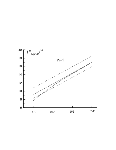
Figure 2: Regge trajectories for Eq. (51) with the potential (52) (solid lines) and for the Salpeter Eq. (55) (dashed lines). In each pair, the lower curve corresponds to $l=j-\frac{1}{2}$ and the upper curve corresponds to $l=j+\frac{1}{2}$.

In Fig. 2 we plot the Regge trajectories for the bound–state Eqs. (51) and (55), as $E^{3/2}$ versus $j$, for the radial quantum numbers $n=0$ (the first plot) and $n=1$ (the second plot). For the bound–state Eq. (51), the trajectories for $j=l\pm\frac{1}{2}$ merge in such a way that at $j=5/2$ the splitting is $0.06$ (in the units of $K_{0}$), whereas for $j=7/2$ it is already $0.01$. Now the BCS scale $\Lambda_{\rm BCS}$ is $0.51K_{0}$. Therefore, if we require that the splitting constitutes a few per cent of $0.51$ (say, about 10 per cent), then the splitting should be below $0.051$, which happens between $j=5/2$ and $j=7/2$, at $E^{3/2}\simeq 11$. This gives the bound–state energy $E\approx 5K_{0}$. Let us define this energy to be the restoration scale $\Lambda_{\rm rest}$. For $j=7/2$ we have a mass splitting which, despite being already fifty times smaller than $\Lambda_{\rm BCS}$, yields a bound–state energy (of $\approx 5.3$) just slightly above $\Lambda_{\rm rest}$. It is then clear that $\Lambda_{\rm rest}$ can be thought of as the onset scale for the chiral restoration regime. In other words: for a mass splitting 10 times smaller than the BCS scale $\Lambda_{\rm BCS}$ we have $\Lambda_{\rm rest}$ 10 times bigger than the BCS scale $\Lambda_{\rm BCS}$,

$$\Lambda_{\rm rest}\approx 5K_{0}\approx 2.5GeV\approx 10\Lambda_{\rm BCS},$$ (57)

where the estimate (47) was used for the parameter $K_{0}$. The result (57) is in good agreement with other estimates of the restoration scale known in the literature Swanson . In Fig. 3 we illustrate, for the sake of completeness, the behaviour of the splitting $\Delta E_{j}=E_{l=j+\frac{1}{2}}-E_{l=j-\frac{1}{2}}$ as a function of the averaged bound–state energy $E_{j}=\frac{1}{2}(E_{l=j+\frac{1}{2}}+E_{l=j-\frac{1}{2}})$.

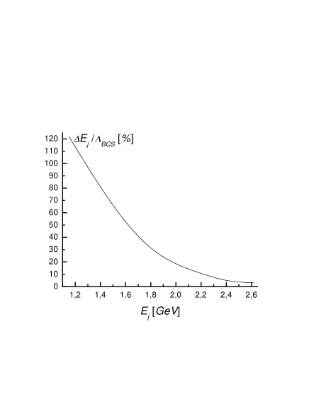
Figure 3: The ratio of the splitting $\Delta E_{j}=E_{l=j+\frac{1}{2}}-E_{l=j-\frac{1}{2}}$ to the BCS scale $\Lambda_{\rm BCS}$, in per cent, versus the averaged bound–state mass $E_{j}=\frac{1}{2}\left(E_{l=j+\frac{1}{2}}+E_{l=j-\frac{1}{2}}\right)$. For the sake of transparency we measure the bound–state energy in $GeV$, using the estimate (47).

In contrast, the trajectories for Eq. (55) remain parallel for all values of the total momentum $j$. This contrast provides an explicit demonstration of the role played for the restoration of the symmetry by the pionic wave function $\sin\varphi_{p}$ in the potential (52).

III.2.3 Generalisation to a generic form of the potential

The results obtained in the framework of the potential quark model (1) are known to be robust against variations of the form of the quark kernel — although the values of various physical quantities might change, for example, with the change of the shape of the confining potential, the relations between such quantities are left intact.

In Fig. 4, for the sake of clarity, we plot the coefficients $C_{p}^{2}$ and $S_{p}^{2}$ versus the relative momentum $p$, measured in $GeV$. To this end we extracted the corresponding scale $K_{0}$, for the given power $\alpha$, from the definition of the BCS scale — see Eqs. (46), (47). This plot is to be compared with the second plot in Fig. 1, where the same quantities are plotted in the units of $K_{0}$. One can see the universality of the behaviour of these functions, regardless of the explicit from of the confining potential. A similar conclusion holds for the dressed quark dispersive law $E_{p}$ which, for excited states in the spectrum, tends to the $\alpha$–independent free–quark limit of $\sqrt{p^{2}+m^{2}}$. We conclude, therefore, that the only ingredient of the bound–state Eq. (28) which changes with the change of the confining potential is the Fourier transform $V({\vec{p}}-{\vec{k}})$, the net result of this change being simply the modification of the Regge trajectory form, from $E^{3/2}$ vs $j$, for the harmonic oscillator potential, for $E^{\frac{\alpha+1}{\alpha}}$ vs $j$, for the generic potential (3). Therefore, we dare to extend the relation (57) beyond the harmonic oscillator potential case of $\alpha=2$, generalising it to the entire family of allowed confining potentials. We find it remarkable that the chiral potential model suggested for studies of chiral low–energy phenomena in QCD appears able to address the problem of the chiral symmetry restoration in the spectrum of highly excited hadrons and to give a reasonable robust prediction for the corresponding restoration scale.

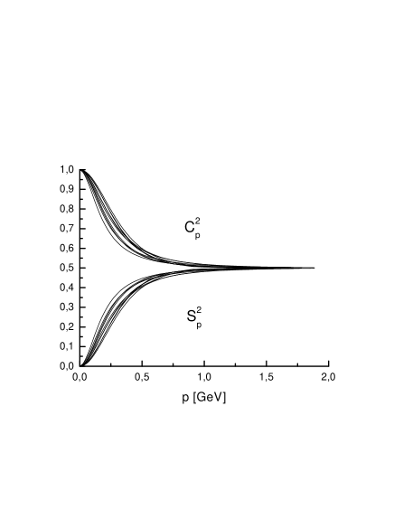
Figure 4: The coefficients $C_{p}^{2}$ and $S_{p}^{2}$ for the potential $V(r)=K_{0}^{\alpha+1}r^{\alpha}$ with various $\alpha$’s (we use the same set of $\alpha$’s as in Fig. 1).

IV Conclusions

In this paper, we investigate the chiral symmetry restoration for highly excited states in the hadronic spectrum. We consider the NJL-type model (1), with an arbitrary confining quark kernel, and use it to study the heavy–light quarkonium. We derive the bound–state equation for the given system in the form of a Schrödingerlike equation and also in the form of an effective Diraclike equation for the light quark in the field of the static antiquark. We give an explicit expression for the matrix structure of the effective interaction of the light quark with the antiquark source for all relative interquark momenta and study the Lorentz nature of this interaction. Thus, we identify explicitly the following three regimes: i) the chiral regime, $p\lesssim\Lambda_{\rm BCS}$, with chiral symmetry breaking playing a dominating role in the interaction — the latter being predominantly scalar, ii) the restoration regime, $\Lambda_{\rm rest}\lesssim p$, which realises for highly excited states in the spectrum, with the effective interaction being vectorial and, as a result, states with opposite parity coming in doublets, and iii) the intermediate regime, which interpolates the two aforementioned ones. We perform a numerical investigation of the heavy–light bound–state equation for the harmonic oscillator potential and demonstrate explicitly the effect of chiral symmetry restoration in the spectrum for orbitally excited states. We estimate the restoration scale to be $\Lambda_{\rm rest}\approx 10\Lambda_{\rm BCS}\approx 2.5GeV$, where the BCS scale $\Lambda_{\rm BCS}$, defining the low–energy properties of the theory, for example, related to the chiral condensate, is chosen to take the standard value of about $250MeV$. Bearing in mind robustness of predictions of the theory (1) for relations between various physical parameters with respect to variations of the quark kernel, we dare to extend this conclusion to an arbitrary confining interquark kernel in the Hamiltonian (1). Thus, we conclude that there is a sufficient window for the intermediate regime in which, on one hand, chiral symmetry does not play a dominating role anymore, whereas, on the other hand, the parity doubling still does not happen in the spectrum. We find that the scale of the chiral symmetry restoration in the spectrum, evaluated in the framework of the potential models (1), is in good agreement with other estimates known in the literature.

- (1) L. Ya. Glozman, Phys. Lett. B 475, 329 (2000); T. D. Cohen and L. Ya. Glozman, Int. J. Mod. Phys. A 17, 1327 (2002); Phys. Rev. D 65, 016006 (2002).
- (2) B. Aubert et al. [BABAR Collaboration], Phys. Rev. Lett. 90, 242001 (2003); D. Besson et al. [CLEO Collaboration], Phys. Rev. D 68, 032002 (2003).
- (3) W. A. Bardeen, E. J. Eichten, and C. T. Hill, Phys. Rev. D 68, 054024 (2003).
- (4) M. Nowak, M. Rho, and I. Zahed, Acta Phys. Polon. B 35, 2377 (2004).
- (5) E. S. Swanson, Phys. Lett. B 582, 167 (2004).
- (6) A. Amer, A. Le Yaouanc, L. Oliver, O. Pene, and J.-C. Raynal, Phys. Rev. Lett. 50, 87 (1983); A. Le Yaouanc, L. Oliver, O. Pene, and J.-C. Raynal, Phys. Lett. B 134, 249 (1984); Phys. Rev. D 29, 1233 (1984).
- (7) P. Bicudo and J. E. Ribeiro, Phys. Rev. D 42, 1611 (1990); ibid., 1635 (1990); P. Bicudo, Phys. Rev. Lett. 72, 1600 (1994); P. Bicudo, Phys. Rev. C 60, 035209 (1999).
- (8) P. Bicudo and J. E. Ribeiro, Phys. Rev. D 42, 1625 (1990).
- (9) A. Le Yaouanc, L. Oliver, S. Ono, O. Pene and J.-C. Raynal, Phys. Rev. D 31, 137 (1985).
- (10) N. Isgur and M. B. Wise, Phys. Lett. B 66, 1130 (1991).
- (11) Y. Nambu, G. Jona-Lasinio, Phys. Rev. 122, 345 (1961).
- (12) S. L. Adler and A. C. Davis, Nucl. Phys. B 244, 469 (1984); Y. L. Kalinovsky, L. Kaschluhn, and V. N. Pervushin, Phys. Lett. B 231, 288 (1989); P. Bicudo, J. E. Ribeiro, and J. Rodrigues, Phys. Rev. C 52, 2144 (1995); R. Horvat, D. Kekez, D. Palle, and D. Klabucar, Z. Phys. C 68, 303 (1995); N. Brambilla and A. Vairo, Phys. Lett. B 407, 167 (1997); Yu. A. Simonov and J. A. Tjon, Phys. Rev. D 62, 014501 (2000); F. J. Llanes-Estrada and S. R. Cotanch, Phys. Rev. Lett. 84, 1102 (2000); N. Ligterink, E. S. Swanson, Phys. Rev. C 69, 025204 (2004).
- (13) Yu. A. Simonov, Yad. Fiz. 60, 2252 (1997) [Phys. Atom. Nucl. 60, 2069 (1997)].
- (14) P. Bicudo, N. Brambilla, E. Ribeiro, and A. Vairo, Phys. Lett. B 442, 349 (1998).
- (15) M. Gell-Mann, R. J. Oakes and B. Renner, Phys. Rev. 175, 2195 (1968).
- (16) M. L. Goldberger and S. B. Treiman, Phys. Rev. 111, 354 (1958).
- (17) S. L. Adler, Phys. Rev. 137, 1022 (1965).
- (18) S. Weinberg, Phys. Rev. Lett. 17, 616 (1966).
- (19) P. Bicudo, S. Cotanch, F. Llanes-Estrada,P. Maris, J. E. Ribeiro, and A. Szczepaniak, Phys. Rev. D 65, 076008 (2002).
- (20) P. Bicudo, Phys. Rev. C 67, 035201 (2003).
- (21) T.-P. Cheng and L.-F. Li, Gauge theories in elementary particles physics (Oxform University Press, London, England, 1984).
- (22) P. Maris and C. D. Roberts, Phys. Rev. C 58, 3659 (1998); M. Bando, M. Harada, and T. Kugo, Progr. Theor. Phys. 91, 927 (1994); C. D. Roberts, Nucl. Phys. A 605, 475 (1996).
- (23) J. Bardeen, L. N. Cooper, and J. R. Schrieffer, Phys. Rev. 106, 162 (1957); ibid. 108, 1175 (1957).
- (24) Yu. S. Kalashnikova and A. V. Nefediev, Yad. Fiz. 62, 359 (1999) [Phys. Atom. Nucl. 62, 323 (1999)]; Usp. Fiz. Nauk 172, 378 (2002) [Phys. Usp. 45, 347 (2002)]; Yu. S. Kalashnikova, A. V. Nefediev, A. V. Volodin, Yad. Fiz. 63, 1710 (2000) [Phys. Atom. Nucl. 63, 1623 (2000)].
- (25) G. ’t Hooft, Nucl. Phys. B 75, 461 (1974).
- (26) I. Bars and M. B. Green, Phys. Rev. D 17, 537 (1978).
- (27) A. V. Nefediev and J. E. F. T. Ribeiro, Phys. Rev. D 70, 094020 (2004).