Electroweak Baryogenesis, Large Yukawas and Dark Matter

Abstract:

It has recently been shown that the electroweak baryogenesis mechanism is feasible in Standard Model extensions containing extra fermions with large Yukawa couplings. We show here that the lightest of these fermionic fields can naturally be a good candidate for cold dark matter. We find regions in the parameter space where the thermal relic abundance of this particle is compatible with the dark matter density of the Universe as determined by the WMAP experiment. We study direct and indirect dark matter detection for this model and compare with current experimental limits and prospects for upcoming experiments. We find, contrary to the standard lore, that indirect detection searches are more promising than direct ones, and they already exclude part of the parameter space.

1 Introduction

The Standard Model (SM) of elementary particles is extremely accurate in describing the fundamental interactions up to the energy scale probed so far at accelerators. Its application to cosmology has led as well to significant successes such as the prediction of the light elements abundance. However the SM fails to provide a pattern to embed all features emerging from recent data on precision cosmology: in particular, neither it does provide a mechanism to explain the origin of the matter-antimatter asymmetry in the Universe, nor it does accommodate a candidate for non-baryonic cold dark matter.

Baryogenesis and the dark matter problem stand as two of the most intriguing topics of research in today’s Science, and they have been examined at length from very different perspectives. It is interesting to notice that, among other viable approaches, both issues have been addressed invoking new physics at the weak scale, at an energy which stands around the corner with respect to upcoming tests of fundamental interactions at present and future accelerators. A successful electroweak baryogenesis [1] can arise in SM extensions in which new particles make the electroweak phase transition strongly first order and add new sources of CP-violation. On the other hand weakly interacting massive particles (WIMPs) are among the leading candidates for dark matter [2]. All these ingredients can be provided in a single framework, as it is the case of supersymmetric extensions of the SM. Even within the minimal supersymmetric SM (MSSM), if the (mostly) right-handed stop is lighter than the top quark and the Higgs is sufficiently light, electroweak baryogenesis may be realized [3] and, at the same time, if the lightest supersymmetric particle is a neutralino, it can play the role of WIMP dark matter candidate.

In a recent paper Carena et al. [4] have shown that in order to strengthen the electroweak phase transition it is not strictly required to consider models with light extra bosonic degrees of freedom, as it was the case in all electroweak baryogenesis models considered in the past, but that models with extra fermions can be equally successful provided that large Yukawa couplings are introduced. A simple implementation of this idea involves introducing doublet and triplet fermions, such as e.g. Higgsinos and gauginos, which can carry as dowry new charge- and color-neutral particles, the lightest of which can be the dark matter candidate. Carena et al. discuss in details one such simple setup, reminding in some aspects split supersymmetry [5], and explicitly show that it can indeed provide electroweak baryogenesis.

In this article we discuss the dark matter features of the above model, as well as those of a slightly extended framework model. Although here, as in the MSSM, the dark matter candidate is a neutralino, the physical state from the superposition of two gaugino and two Higgsino fields, we point out that there are significant differences compared to the MSSM case, both in the mechanism setting its thermal relic density and in its phenomenology as dark matter candidate. In particular we show that currently the tightest constraint on the model comes from limits on the neutrino induced flux from pair annihilation of dark matter neutralinos gravitationally trapped in the center of the Sun. We also show that the best option for the upcoming future is to measure an excess in antimatter cosmic ray fluxes, while direct detection in underground laboratories looks less promising.

The plan of the paper is as follows. In Section 2 we review the framework introduced in Ref. [4] and discuss relevant features from the perspective of the dark matter problem. In Section 3 we discuss how dark matter candidates arise in a model with a reduced number of parameters, for which the baryogenesis mechanism was discussed in detail in Ref. [4]. In Section 4 we present limits on the model from current searches and future perspectives, going through all the techniques of WIMP dark matter detection. In Section 5 we discuss the dark matter thermal relic density and current and future searches in a more generic model, within the framework discussed in detail in Ref. [4], where future direct detection is more promising. Finally our conclusions are drawn in Section 6.

2 Particle physics framework

We consider a minimal extension of the SM in which the role of the extra fermions with large Yukawa couplings is played by fields with the quantum numbers of Higgsinos and gauginos in supersymmetric theories; such fields are assumed to be the only light extra particles present in our theory and relevant for its weak-scale phenomenology. Our extra fields have gauge interactions as ordinary Higgsinos and gauginos in the MSSM, while we define their couplings to the SM Higgs doublet $H$ through the Lagrangian:

$$\mathcal{L} = H^{\dagger}\left(h_{2}\,\sigma_{a}\tilde{W}^{a}+h^{\prime}_{2}\,\tilde{B}\right)\tilde{H}_{2}+H^{T}\epsilon\left(-h_{1}\,\sigma_{a}\tilde{W}^{a}+h^{\prime}_{1}\,\tilde{B}\right)\tilde{H}_{1}$$ (1)

$$+ \frac{M_{2}}{2}\,\tilde{W}^{a}\tilde{W}^{a}+\frac{M_{1}}{2}\,\tilde{B}\tilde{B}+\mu\,\tilde{H}^{T}_{2}\epsilon\tilde{H}_{1}+h.c.\;,$$

with $\epsilon=i\,\sigma_{2}$. The setup we have introduced has a particle content analogous to the split supersymmetry scenario, a MSSM in which all scalars, except for the SM-like Higgs, are driven at a very heavy mass scale. Hence one could regard it as a particular realization of split supersymmetry in which the standard relation between gauge and Yukawa couplings has been spoiled . Another difference being that in split supersymmetry the gluino may be light, with relevant phenomenological implications but unrelated to the dark matter or baryogenesis problems at focus here. For reference, ordinary MSSM couplings are recovered if the generic Yukawa couplings $h_{1,2}$ and $h^{\prime}_{1,2}$ are chosen as:

$$h_{1}=g\cos\beta/\sqrt{2} h_{2}=g\sin\beta/\sqrt{2}$$

$$h_{1}^{\prime}=g^{\prime}\cos\beta/\sqrt{2} h_{2}^{\prime}=g^{\prime}\sin\beta/\sqrt{2}$$ (2)

where $g$ and $g^{\prime}$ are the $SU(2)$ and $U(1)$ gauge couplings. Modifications to these relations can appear in other non-minimal contexts. Keeping this in mind, we will take the Yukawa couplings as free parameters and we will discuss the phenomenology of the model regardless of its eventual supersymmetric completion at high energy.

Four physical neutral states $\tilde{\chi}^{0}_{i}$ and two physical charged states $\tilde{\chi}^{\pm}_{i}$ are obtained by diagonalizing the corresponding mass matrices. According to our definitions, in the basis $\left(\tilde{B}^{0},\tilde{W}^{0},\tilde{H}^{0}_{1},\tilde{H}^{0}_{2}\right)$, the neutralino mass matrix takes the form:

$$\left(\begin{array}[]{cccc}M_{1}&0&-\sqrt{2}\,h_{1}^{\prime}\,m_{W}/g&\sqrt{2}\,h_{2}^{\prime}\,m_{W}/g\\ 0&M_{2}&\sqrt{2}\,h_{1}\,m_{W}/g&-\sqrt{2}\,h_{2}\,m_{W}/g\\ -\sqrt{2}\,h_{1}^{\prime}\,m_{W}/g&\sqrt{2}\,h_{1}\,m_{W}/g&0&-\mu\\ \sqrt{2}\,h_{2}^{\prime}\,m_{W}/g&-\sqrt{2}\,h_{2}\,m_{W}/g&-\mu&0\end{array}\right)\;$$ (3)

while the chargino mass matrix is:

$$\left(\begin{array}[]{cc}M_{2}&2\,h_{2}\,m_{W}/g\\ 2\,h_{1}\,m_{W}/g&\mu\end{array}\right)\;.$$ (4)

Since baryogenesis stands as the main motivation of our framework, we need to introduce a non-vanishing CP-violating phase, triggering baryon number generation: as a minimal assumption, it is sufficient to take the Higgsino mass parameter to be complex, $\mu=|\mu|\,e^{i\varphi}$, while choosing the gaugino mass parameters $M_{1}$ and $M_{2}$, and the Yukawa couplings to be real.

2.1 Lightest neutralino mass and composition

We focus on the case in which the lightest neutralino (LN) $\tilde{\chi}^{0}_{1}$ is the lightest extra-fermion (LEF) and hence a stable species : the LN being electric- and color-charge neutral, massive and stable it is an ideal candidate for cold dark matter. The phenomenology of the LN as a dark matter candidate crucially depends on its mass and mixing; in particular, the relative weight between its gaugino and Higgsino components is decisive both in setting the LN thermal relic abundance and in determining the detection prospects of such a model.

The gaugino or Higgsino nature of the LN is related as usual to the hierarchy among the parameters $M_{1}$, $M_{2}$ and $\mu$. Since in our model there are significant differences compared to the most commonly considered cases in the MSSM context, we preliminarily sketch here some trends in a few sample cases in which it is possible to diagonalize analytically the neutralino mass matrix.

As a first example we focus on the setup in which $M_{1}$ is very heavy, i.e. $|M_{1}|\gg|\mu|,|M_{2}|,\sqrt{2}\,h_{1,2}\,m_{W}/g$, and hence the $\tilde{B}^{0}$ component decouples. For simplicity we also assume that $\mu$ is real and $h_{1}=h_{2}\equiv h$ . In this case the three light eigenvalues of the neutralino mass matrix are:

$$\lambda_{\pm}={1\over 2}\left(M_{2}+\mu\pm\sqrt{(M_{2}-\mu)^{2}+16\,h^{2}m_{W}^{2}/g^{2}}\right)\;,\;\;\;\;\;\;\lambda_{3}=\mu\;.$$ (5)

In the limit $|\mu|\gg|M_{2}|$, the lightest eigenvalue is $\lambda_{-}\simeq M_{2}-4\,h^{2}\,m_{W}^{2}/g^{2}\mu$ and the associated eigenvector is mostly Wino-like, with a Higgsino component induced by the Yukawa term which gets smaller and smaller as the $M_{2}$ scale gets much larger than $h\,m_{W}/g$ (recovering the limit one would have in the MSSM). In the opposite regime $|\mu|\ll|M_{2}|$ there are two light states: $\lambda_{-}\simeq\mu-4\,h^{2}\,m_{W}^{2}/g^{2}M_{2}$ and $\lambda_{3}=\mu$. If $\mu$ and $M_{2}$ have the same sign the first state is the lightest one and the associated LN is mostly Higgsino-like, with a Wino component again introduced by the Yukawa terms. If $\mu$ and $M_{2}$ have opposite signs the state with mass $\lambda_{3}$ becomes the lightest one and now the LN is an almost pure Higgsino state. These three regimes and the corresponding LN compositions are schematically summarized in the left panel of Fig. 1, in the plane $(\mu;\,M_{2})$ and for the sample value $h=1$.

 

Figure 1: The gaugino and Higgsino contents of the lightest neutralino in the plane ($\mu;\,M_{2}$). We label pure Higgsino (gaugino) the state with a Higgsino (gaugino) component greater than 90%. A mostly Higgsino (gaugino) state has a Higgsino (gaugino) component between 50% and 90%. We assume Yukawa couplings $h=1$ as sample reference value. In the left panel $M_{1}$ has been fixed at a very heavy scale; in the right panel we assumed $M_{1}=M_{2}$.

Another simple case showing the interplay between mass parameters and mixings can be built by choosing e.g. $M_{1}=M_{2}=M$ and $h_{1,2}=h_{1,2}^{\prime}=h$ (still $\mu$ is taken to be real). In this case the eigenvalues of the neutralino mass matrix are:

$$\lambda_{\pm} = {1\over 2}\left(M+\mu\pm\sqrt{(M-\mu)^{2}+32h^{2}m_{W}^{2}/g^{2}}\right)\;,$$

$$\lambda_{3} = M\;,\;\;\;\;\;\;\lambda_{4}=\mu\;.$$ (6)

Again the state with mass $\lambda_{4}$ is almost pure Higgsino with mass $\mu$, while that with mass $\lambda_{3}$ is an almost pure gaugino state with mass $M$. Due to the Yukawa coupling this gaugino state is a mixing between the Bino and the Wino in the same percentage . As in the previous example the remaining states with masses $\lambda_{\pm}$ are gaugino-Higgsino mixed states with relative weight depending on the values of the parameters. The hierarchy between eigenvalues is analogous to the previous case, except that now the state with mass $\lambda_{-}$ becomes the lightest one only in the case where both $\mu$ and $M$ are fairly large. Regions of different LN compositions are shown in Fig. 1, right-panel. Note there is a region in the parameter space in which the LN is not the lightest extra fermion, since a chargino becomes lighter.

Another case we will consider later on regards the possibility to fix the ratio between the gaugino mass parameters, i.e. $M_{1}=\alpha M_{2}$. The general trend here is very similar to the previous one, taking into account that by varying the parameter $\alpha$ we change the Bino content of the gaugino-like LN. At the same time in the limit $\alpha\gg 1$ one recovers the complete Bino decoupling as in the first case discussed here, except for the corner at very small $M_{2}$, where $M_{1}\gg h\,m_{W}/g$ does not hold any more and hence the Bino does not decouple.

3 Dark matter candidates in a guideline model

Analogously to the MSSM with $R$-parity conservation, in our scenario the lightest extra fermion $\widetilde{\chi}^{0}_{1}$ is stable, massive and weakly interacting, and hence a natural WIMP candidate for cold dark matter (CDM). We compute the LN thermal relic density by interfacing the particle physics framework we have introduced in the DarkSUSY package [6]. Such package allows for high accuracy solutions of the Boltzmann equations describing thermal freeze out. In particular, in computing thermally-averaged LN pair annihilation cross-sections , all kinematically allowed final states are systematically included, as well as eventual co-annihilation effects . The density evolution equation is then solved numerically. The estimated precision on the value of the relic density we derive is, for a given set of input parameters setting masses, widths and couplings, of the order of 1% or better. The LN relic density value is to be compared with the latest determination of the CDM component of the Universe by the WMAP experiment [7]: $\Omega_{CDM}h^{2}=0.113\pm 0.009$.

Our first working model within the framework will be that with a reduced number of parameters discussed at length in Ref. [4] in the electroweak baryogenesis context. We first take the limit of Bino decoupling setting $|M_{1}|\gg|\mu|,|M_{2}|$ and $h_{1,2}^{\prime}=0$, and then fix $\mu=-M_{2}\,e^{i\varphi}$, a condition which maximizes the number of degrees of freedom contributing to strengthening the electroweak phase transition. For this particular model it has also been explicitly shown that one can build an ultraviolet completion canceling out instabilities in the zero temperature Higgs potential induced by the light extra fermions we have introduced . Our guideline model is then defined by only five free parameters: $|\mu|$, $\varphi$, $h_{+}=\frac{1}{2}\left(h_{1}+h_{2}\right)$, $h_{-}=\frac{1}{2}\left(h_{1}-h_{2}\right)$ and the SM Higgs mass $m_{H}$. Going back to the list of limiting cases we discussed in the previous Section, we see that we are referring to a model in which the LN is an almost pure Higgsino with mass $M_{LN}\simeq|\mu|$.

Figure 2: Sample isolevel curves of the lightest neutralino relic abundance at the currently preferred value $\Omega_{LN}h^{2}=0.113$. From top to bottom the extra free parameters are set equal to: $h_{+}=2$, $\varphi=0$ and $m_{H}=300$ GeV (thick dashed curve), $h_{+}=2$, $\varphi=0$ and $m_{H}=150$ GeV (thin dashed curve), $h_{+}=1.5$, $\varphi=0$ and $m_{H}=150$ GeV (solid curve), $h_{+}=2$, $\varphi=\pi/2$ and $m_{H}=150$ GeV (dash-dotted curve), and $h_{+}=1.5$, $\varphi=\pi/2$ and $m_{H}=150$ GeV (dotted curve).

In Fig. 2 we show isolevel curves at $\Omega_{LN}h^{2}=0.113$ in the plane $(|\mu|;\,h_{-})$, for a few sample values of $\varphi$, $h_{+}$ and $m_{H}$. The relic density is sensitive to the parameter $|\mu|$ since it drives the mass scales of the extra particles we have introduced. We are restricting ourselves to the case $h_{-}<0$, since the model is symmetric under the exchange $h_{-}\rightarrow-h_{-}$. The value of the relic density rapidly changes with $h_{-}$ because, as pointed out in Ref. [4], the coupling $Z^{0}\widetilde{\chi}^{0}_{1}\widetilde{\chi}^{0}_{1}$ is proportional to:

$$g_{Z^{0}\widetilde{\chi}^{0}_{1}\widetilde{\chi}^{0}_{1}}\propto\frac{h_{2}^{2}-h_{1}^{2}}{h_{2}^{2}+h_{1}^{2}}=-\frac{1}{2}\frac{h_{+}\,h_{-}}{h_{-}^{2}+h_{+}^{2}}\,.$$ (7)

At values of the $\widetilde{\chi}^{0}_{1}$ mass below the threshold for pair annihilation into gauge boson final states, the only open channel is the helicity suppressed fermion-antifermion state, which gets its largest contribution from the diagram with a $Z$ boson in the $s$-channel. The annihilation rate gets maximal on resonance, at $m_{\widetilde{\chi}^{0}_{1}}=m_{Z}/2$, driving the relic density to very small values unless one considers a tiny $h_{-}$. Moving away from the resonance, both toward heavier and lighter masses, the isolevel curves spread out to larger and larger values of $h_{-}$. We only display in Fig. 2 the upper branch since, for LN masses smaller than $m_{Z}/2$, the induced contribution to the $Z$ invisible width is larger than the experimental upper bound and such models are excluded by LEP results. For LN masses approaching the $W$ and $Z$ masses, LN pair annihilations into $W^{+}\,W^{-}$ and $Z^{0}\,Z^{0}$ in the early Universe become relevant and tend eventually to dominate. These processes proceed mainly through $t$- and $u$-channel exchanges of, respectively, the lightest chargino (LC) and the next-to-lightest neutralino (NLN).

At first sight this picture may just seem the analogue to the well-studied case of Higgsinos in the MSSM; there are however substantial differences. In the MSSM, in the case of a pure Higgsino LN, the lightest chargino and the next-to-lightest neutralino are quasi-degenerate in mass with the LN: the contribution of the $W^{+}\,W^{-}$ and $Z^{0}\,Z^{0}$ final states to the cross-section becomes too large as soon as the LN mass gets above the corresponding threshold, driving the relic abundance to very small values . To compensate for this, one should increase the Higgsino LSP mass up to the TeV range.

 

Figure 3: Left panel: The mass splitting between the lightest neutralino (LN) and the lightest chargino (LC) or the next-to-lightest neutralino (NLN), defined as $\Delta_{i}=\left(m_{i}-m_{LN}\right)/{m_{LN}}$, as function of $\mu$. We assumed $h_{+}=2$, with $\varphi$ between extrema, and chosen $h_{-}=-0.25$ (there is a mild shift in the mass splittings varying $h_{-}$ in the interesting range for the relic abundance). Right panel: Cross-section for LN pair annihilation into a $W$-boson pair, in the limit of particles in the initial state at rest, as function of the lightest neutralino mass. The solid line corresponds to the computation made with DarkSUSY, the dashed line to the result assuming pure Higgsino couplings and a mass of the lightest chargino equal to 300 GeV (average value of $m_{LC}$ in the sample parameter choice).

On the other hand, in our framework, while $m_{\widetilde{\chi}^{0}_{1}}\simeq|\mu|$, the mass scale of the other two fermionic states is instead set by the largest of the Yukawa terms $h_{1}$ and $h_{2}$, or equivalently by $h_{+}$, and the mass splittings can be very large. This is shown in the left panel of Fig. 3; the parameters $\varphi$ and $|h_{-}|$ contribute as well in setting the mass splittings, but at a milder level. It follows that, along the foliation of the parameter space we are considering, at a fixed value of $h_{+}$ and varying $|\mu|$, the rate of annihilation into gauge bosons increases with the LN mass (i.e. with $|\mu|$), rather than decreasing with it as one would intuitively expects and happens e.g. in the MSSM. This trend is shown for the $W^{+}\,W^{-}$ final state in the right panel of Fig. 3. The mass dependence we find for $\sigma v$ closely reproduces the scaling $m_{\widetilde{\chi}^{0}_{1}}^{2}/m_{LC}^{4}$ we have displayed (dashed line) implementing the formula for the cross-section for a pure Higgsino coupling and fixing $m_{LC}$ to the mean value in our sample parameter choice.

Coming back to Fig. 2, once above the threshold for gauge boson production the isolevel curves bend back to the (small) values of $|h_{-}|$ at which, for given $|\mu|$, $h_{+}$ and $\varphi$ (and hence the corresponding LN–LC and LN–NLN mass splittings), diagrams with a chargino or neutralino exchange alone are large enough to drive the relic abundance down to the WMAP range. At larger values of $|h_{-}|$ the large coupling between LN and the $Z$ boson makes the $W$ boson final state to get an additional large contribution from the diagram with the $Z$ boson in the $s$-channel. In each sample case the region delimited by the isolevel curve and the vertical axis at $h_{-}=0$ corresponds to relic densities larger than the central value from the WMAP determination (i.e. most of it is cosmologically excluded), while at larger $h_{-}$ (i.e. outside the region delimited by the isolevel curves) relic densities are lower than the value required for the LN to be the main dark matter component . Modifications to the general trend we sketched come from eventual additional contributions when other final states become kinematically allowed. In the examples with $h_{+}=2,\,\varphi=0$, mass splittings between the extra fermions are the largest ones and the isolevel curves stretch for LN masses above the top mass: the process $\widetilde{\chi}^{0}_{1}\widetilde{\chi}^{0}_{1}\rightarrow t\overline{t}$ comes into play and, since this channel is not helicity suppressed, it gets large contributions through the s-channel Z exchange down to very small values of $|h_{-}|$, $|h_{-}|\simeq 5\times 10^{-2}$. If the $Z^{0}H$ final state becomes kinematically allowed, it can give as well a substantial contribution to the annihilation cross-section. This effect is shown again for the two curves with $h_{+}=2,\,\varphi=0$: one with $m_{H}=150$ GeV, i.e. close to the presently preferred value from electroweak precision measurements [8], the other with $m_{H}$ twice as large. For $m_{H}=150$ GeV the $Z^{0}H$ threshold opens up at $|\mu|\sim 120$ GeV: above it the two isolevel curves depart from each other, while below it the curves essentially coincide since $H$ enters only through contributions to s-channel diagrams, always much smaller than the corresponding $Z^{0}$ s-channel diagram. In the same way, the shape of the isolevel curves for $h_{+}=1.5,\,\varphi=\pi/2$ and $h_{+}=2,\,\varphi=\pi/2$ remains essentially unchanged in case we rise the value $m_{H}=150$ GeV to much larger values.

The sample cases we have considered, with fairly large $h_{+}$  and moderately light $m_{H}$ are among those found to be favored by electroweak baryogenesis in Ref. [4], and hence they are good cases to check the phenomenology of the dark matter model in the framework where the baryogenesis problem is simultaneously addressed. At the same time, the size of the CP-violating phase has been varied freely between extremes, and will enter in our discussion through the shift in mass splittings only. For transparency in our discussion, and to present results which have a validity on their own, we are not going to zoom in only sub-slices of the parameter space which are fully successful in electroweak baryogenesis. In the same vein, we implement as sharp cut to the parameter space only the bound on extra contributions to the $Z$ invisible width. As it was discussed in Ref. [4], significant constraints on the model can be extracted also from experimental bounds on the electroweak $T$-parameter: the slice of models included in our plot at the largest value of $|h_{-}|$ are excluded for small values of $m_{H}$, while the constraint gets weaker going to a heavier Higgs. On the other hand, as it was shown in the relic density calculation and discussed further below, the phenomenology of the dark matter candidate is almost insensitive to $m_{H}$, except for the threshold effect already described. We will keep all models and show that actual current limits on dark matter searches introduce even tighter constraints, independently on the value of $m_{H}$.

4 Detection rates in the guideline model

The issue of WIMP dark matter detection has been studied at length (for reviews see e.g. [9, 10]). We will systematically go through all WIMP detection techniques to illustrate those that already exclude models within our framework and what are the detection prospects for the future. As for the relic density, all rates are computed with the DarkSUSY package [6]. The set of underlying assumptions is briefly reviewed here, while present limits and the future outreach is discussed within the simplified framework of our guideline model.

4.1 Direct detection

In the last decade considerable resources have been invested in the attempts to directly detect WIMPs, i.e. to measure the energy deposited in elastic scatterings off of nuclei by dark matter WIMPs passing through the target material of a detector [11]. We present predictions in terms of scattering cross-sections on a single nucleon, separating as usual the term accounting for coherent spin-independent (SI) interactions from the one due to axial-vector spin-dependent (SD) coupling. In our framework the process of scattering of a LEF on a quark is particularly constrained since only a $t$-channel exchange of the SM Higgs boson mediates the SI part, while only the diagram with $Z^{0}$ boson gives a contribution to the SD one. To convert coupling on quarks into couplings on nucleons we refer to a standard set of parameters [12, 13] for nucleonic matrix elements .

 

Figure 4: The spin-independent cross-section on a proton (left panel) and the spin-dependent cross-section on a neutron (right panel) versus the lightest neutralino mass, as compared to current exclusion curves (CDMS II) and the projected sensitivity of future detectors (SuperCDMS). The models displayed are those at $\Omega_{LN}h^{2}=0.113$ singled out in Fig. 2, with the same sample choice of parameters and the same line-type (color) coding. Note the mismatch in the vertical scale of the two plots.

In the left panel of Fig. 4 we plot predictions for the SI neutralino-proton scattering cross-section $\sigma_{\chi P}^{\rm SI}$, as a function of the LEF mass. Models we display are those singled out in Fig. 2 at $\Omega_{LN}h^{2}=0.113$, with the same sample parameters and coding therein. For comparison we have shown the exclusion curve from the null search by CDMS II [15] and the future expected sensitivity of the SuperCDMS project in its one ton configuration [16] . As it can be seen predictions are orders of magnitude below current sensitivities, as well as far below projected future sensitivities, as one could have foreseen from the features of the slice in the parameter space we have zoomed in. In fact as already mentioned $\sigma_{\chi P}^{\rm SI}$ has one single contribution mediated by a Higgs exchange, which is largely suppressed since the $\widetilde{\chi}^{0}_{1}\widetilde{\chi}^{0}_{1}H$ vertex scales with the gaugino-Higgsino mixing in $\widetilde{\chi}^{0}_{1}$: in our guideline model the LN is always a very pure Higgsino, its gaugino content going to zero in the limit $h_{-}\rightarrow 0$, and it is of the order of few percent even for the largest $|h_{-}|$ reached in Fig. 2 (the peaks in each of the displayed curves). In all but one case we are considering a rather light Higgs, $m_{H}=150$ GeV. Since the cross-section scales with the inverse of its forth power, taking $m_{H}$ equal to its current lower limit ($\sim 115$ GeV) one only gains a factor of about 3 in the cross-section. Actually considering a heavier Higgs the prediction gets rapidly further suppressed, as it can be seen by comparing the case we plot with $m_{H}=300$ GeV (thick dashed line) with the corresponding one at $m_{H}=150$ GeV (thin dashed line).

In the right panel of Fig. 4 we instead plot the predictions for the SD neutralino-neutron scattering cross-section $\sigma_{\chi N}^{\rm SD}$ . Here the picture looks more promising since now the cross-section scales with the coupling of the LN with the $Z$-boson, i.e. the same effect setting, to some extent, the LN relic density. Again in each plot of $\sigma_{\chi N}^{\rm SD}$ versus mass there are maxima corresponding to the largest values of $|h_{-}|$ along each isolevel curve. Such maxima are again well below current sensitivities (the best exclusion curve being again set by the CDMS II result [18]), however perhaps within the reach of future detectors. The CDMS Collaboration is performing its DM searches with natural $Ge$, which has a small component (around 8%) of the ${}^{73}Ge$ isotope, a target with an unpaired neutron from which the limit on $\sigma_{\chi N}^{\rm SD}$ has been derived. We can derive a rough projection for the gain in sensitivity on SD couplings by simply scaling down the current exclusion curve of SuperCDMS regarding the SI coupling in Ref. [16] and shown in the left panel . We find that a substantial fraction of the models along the $\Omega_{LN}h^{2}$ isolevel curves in our guideline framework, down to masses close to 50 GeV, will be detectable by SuperCDMS or by an equivalent experiment.

4.2 Neutrino telescopes

Figure 5: Muon flux induced by the neutrino flux from LN pair annihilations in the center of the Sun versus LEF mass, and comparison with the current best exclusion curve (SUPER-KAMIOKANDE) and the projected sensitivity of future detectors (IceCube). The models displayed are those at $\Omega_{LN}h^{2}=0.113$ singled out in Fig. 2, with the same sample choice of parameters and the same color (line-type) coding.

The search for neutrinos produced by the annihilation of neutralinos trapped in the core of the gravitational wells of the Sun or of the Earth is a very promising indirect detection technique since it has a very distinctive signature, and potentially induced fluxes may be large. In the present framework, since spin-independent cross-sections are small, capture rates and fluxes from the Earth are actually very low and will not be considered further. To estimate neutrino fluxes from the Sun we implement the standard procedure described in Refs. [10, 19], except for a more careful treatment of neutralino capture rates [20, 6]. In Fig. 5, we present results in terms of muon-induced fluxes, above the threshold of 1 GeV, and compare them to the current best limits from the SUPER-KAMIOKANDE Collaboration [21] and with the future projected sensitivity of the IceCube experiment [22] . The color coding on the $\Omega_{LN}$ isolevel curves is the same as in Figs. 2 and 4. Since the capture rate in the Sun is driven by the SD neutralino-proton coupling, and we have just verified that this can be fairly large, we find that a large portion of LN models in our guideline scenario sharply overshoots the currently best exclusion curve, and that there are fair chances of detection with the improved sensitivity of IceCube. The muon-induced fluxes sharply increase at the $W$ threshold, since LN annihilations at zero temperature into gauge boson final states (which are a copious source of high energy neutrinos) is not helicity suppressed as it happens for the $b\,\bar{b}$ final state which dominates at lower masses.

Summarizing our result we find that, in the present guideline framework, LN dark matter models slightly heavier than the $W$ mass along the $\Omega_{LN}h^{2}$ isolevel curves corresponding to $|h_{-}|\stackrel{{\scriptstyle>}}{{{}_{\sim}}}0.15$ are already excluded by current limits. This conclusion essentially holds independently of the choice of the parameter $m_{H}$ (compare the thick and thin dashed curves which differ only in the value of $m_{H}$). In the future, with neutrino telescopes it will be possible to test models at smaller values of $h_{-}$ in the heavier mass branch, covering a region of parameter space larger than the one expected from spin-dependent couplings in direct detection. On the other hand since upcoming neutrino telescopes have a high energy threshold no progress is foreseen in the light mass branch where, instead, direct detection in the future will be more competitive.

4.3 Halo rates

Lightest neutralino pair annihilations in the Galactic halo may be a significant source of cosmic-ray and gamma-ray fluxes. We will mainly focus on the first ones and mention gamma-rays at the end of the Section.

Charged particles injected in the Galaxy get trapped in the interstellar magnetic fields building up an equilibrium population and diffusing up to the solar system and the Earth where they can be detected. Since there is no evidence of standard primary sources of antimatter, and antimatter of secondary origin is scarce, searching for antimatter from dark matter pair annihilations is a promising technique to test the dark matter paradigm. We will consider the induced antideuteron, antiproton and positron fluxes.

Figure 6: Reduced $\chi^{2}$ for the fit of presently available antiproton flux data with a background plus neutralino signal, as a function of lightest neutralino mass and within models singled out in Fig. 2. The 3 $\sigma$ discrimination level is shown as a horizontal line. The adiabatically contracted halo profile has been assumed in this computation: considering the Burkert profile, the signal becomes a small correction over the background and no model can be discriminated.

Predictions involve several elements: the particle physics setup fixes the pair annihilation cross-section $\sigma_{\rm ann}v$ and the branching ratios for the various annihilation channels. For each of them fragmentation and/or decay processes give rise to the stable antimatter species, a step we include using tabulated results from the Pythia [23] 6.154 Monte Carlo code as included in the DarkSUSYpackage, except for $\bar{D}$ sources for which we have implemented the prescription suggested in Ref. [24] to convert from the $\bar{p}$-$\bar{n}$ yields. To complete the estimate of the strength of dark matter sources, one needs the number density of neutralino pairs locally in space, i.e. in terms of the dark matter density profile $\rho$ and the dark matter particle mass $m_{LN}$, as $1/2\,(\rho(\vec{x}\,)/{m_{LN}})^{2}$. The choice of the halo profile is then crucial in the prediction of fluxes: we will consider two possible setups ranging from the most favorable one for dark matter detection to one of the least favorable ones.

For the first choice, which we will refer as the adiabatically contracted model, we consider a model obtained by assuming that the dark matter profile of the Milky Way, before gas cooling and the formation of its luminous components, is described by the universal profile found in Ref. [25] resulting from N-body simulations of hierarchical structure formation in a $\Lambda$CDM cosmology, with mass $M_{vir}=1.8\times 10^{12}M_{\odot}{\ }$ and concentration parameter $c_{vir}=12$. The baryon infall is included assuming a smooth and slow process, with a further enhancement of the dark matter density in the central portion of the Galaxy (adiabatic contraction limit with no redistribution of angular momentum between its components [26]). The central portion of the profile becomes as steep as $1/r^{1.5}$, but this singularity has been conservatively cut off in its innest 1 pc, corresponding to a core radius [27, 28] which is possibly induced by one of the scenarios for the formation of the black hole sitting at the center of the Galaxy [29].

The second halo model we consider is defined by a profile with a large core radius, a Burkert profile [30] with $M_{vir}=1.3\times 10^{12}M_{\odot}{\ }$ and $c_{vir}=16$. We can think about this case as the limit in which the profile is reshaped by a large redistribution of angular momentum during the baryon infall, with the inner density being sensibly reduced. Both profiles are assumed to be spherical and to have analogous values of the local halo density, $0.38$ GeV cm^-3 and $0.34$ GeV cm^-3, respectively. Hence predictions in direct and indirect detection with neutrino telescopes do not change appreciably and we have not anticipated this discussion . The analysis could be more articulated including effects e.g. of substructures giving further enhancements in the predictions. However we will not consider this possibility here, and instead we will take a more conservative approach.

The last step to make a prediction for the antimatter fluxes is to model the propagation in the intergalactic magnetic fields and against the solar wind within the solar system. The propagation model adopted for antiprotons and antideuterons has been developed in Ref. [31] and that for positrons in Ref. [32]. Free parameters in both cases are set in analogy to a setup which has been shown to reproduce fairly well the ratios of primary to secondary cosmic ray nuclei [33] with the Galprop [34] propagation code. Solar modulation is instead sketched with the analytical force-field approximation [35], with a modulation parameter as appropriate at each phase in the solar cycle activity.

We first compare the prediction for the antiproton flux against a compilation of data collected in the latest years. We consider results with the BESS experiment that has measured with fairly good statistics the antiproton flux in the energy range between 180 MeV and 4.2 GeV during its flights in 1997, 1998, 1999 and 2000 [36], and those in the range between 3 and 50 GeV obtained by the CAPRICE experiment during its 1998 flight [37]. The expected component from neutralino annihilations is added to the secondary component due to cosmic-ray interactions, again estimated with the Galprop [34] code under the same setup implemented for the neutralino-induced component, that yields $\chi^{2}=0.82$. Values of the reduced $\chi^{2}$ for the case signal plus background are shown in Fig. 6, in the case of models along the sample isolevel curves singled out in Fig. 2 and for a distribution of dark matter particles according to the adiabatically contracted profile. Some of the models give values of the reduced $\chi^{2}$ as large as a few and are most probably excluded by antiproton measurements. One should note however that the 3 $\sigma$ exclusion level at about 1.4 should not be considered a strict bound since we have not taken into account uncertainties in the propagation model and other steps in our prediction. At the same time the limits we show are very sensitive to our halo choice: if the more conservative Burkert halo is instead considered all signals get suppressed by a factor of $\sim 100$, becoming a small correction with respect to the background and leaving no chance of discrimination with current data.

 

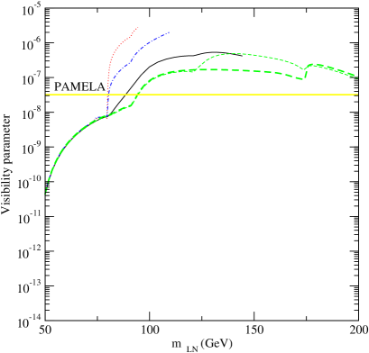
Figure 7: Visibility parameter for future antiproton (left panel) and positron (right panel) searches as compared to the detection perspectives with the PAMELA instrument. The models displayed are those at $\Omega_{LN}h^{2}=0.113$ singled out in Fig. 2, with the same sample choice of parameters and the same color (line-type) coding. Predictions are shown in case of the adiabatically contracted halo profile.

Perspectives for the future are sketched in the left panel of Fig. 7. The quantity plotted on the vertical axis is

$$I_{\Phi}\equiv\int_{E_{min}}^{E_{max}}dE\,\frac{\left[\Phi_{s}(E)\right]^{2}}{\Phi_{b}(E)}\,,$$ (8)

where $\Phi_{s}(E)$ and $\Phi_{b}(E)$ are the signal and background fluxes, respectively, and the integral extends over the whole interval in which the ratio is non negligible. It gives the continuum limit of a $\chi^{2}$-like variable in the regime in which the signal is a small correction to some known background, see Ref. [39] for details. In Fig. 7 the horizontal line gives, in this same variable, the discrimination level which will be reached by the PAMELA experiment [38] in three years of data taking (which should start in early 2006). The predictions are for the adiabatically contracted profile and they indicate that in such setup all models with the LN heavier than the $W$ gauge boson, even those with extremely small $|h_{-}|$, would be tested. This signal, as all halo signals, scales with the total annihilation rate at zero temperature which for gauge boson final states is unsuppressed and little related to the coupling of the LN with the $Z^{0}$, unlike in the case of lower masses and fermion final states. Again we must stress that this conclusion heavily relies on which halo profile is chosen: if the Burkert profile is implemented, predictions for the parameter $I_{\Phi}$ are shifted down over two orders of magnitude, and no model would be tested even in the future within such a setup.

In the right panel of Fig. 7 we show the analogous picture for the positron fluxes. The range of models which will be testable in the future, for the adiabatically contracted profile, is in this case slightly smaller than in the antiproton case. Limits from current data do not allow any model discrimination even with this halo model, and hence the analogue of Fig. 6 is not shown.

 

Figure 8: Visibility ratio for future antideuteron searches with the GAPS instrument (all models above the horizontal line are detectable), in case of a mission with a satellite on an earth orbit. The distribution of neutralinos in the halo has been assumed according to the adiabatically contracted model (left panel) or the Burkert profile (right panel). The models displayed are those at $\Omega_{LN}h^{2}=0.113$ singled out in Fig. 2, with the same sample choice of parameters and the same color (line-type) coding. Values of the visibility ratio shift up by a factor of about 3 if one considers the same instrument placed on a deep space probe.

At present there are no data on the antideuteron cosmic ray flux and indeed, if one constrains oneself to the low energy window, the secondary background flux is expected to be negligible [24], so that even the detection of one single event could be used to claim the presence of an exotic primary source. To address the detection prospects for the future we consider the gaseous antiparticle spectrometer (GAPS) [40], which will have the capability of searching for antideuterons in the energy interval 0.1-0.4 GeV per nucleon, with an estimated sensitivity level of $2.6\times 10^{-9}\textrm{m}^{-2}\textrm{sr}^{-1}\textrm{GeV}^{-1}\textrm{s}^{-1}$, and that has been proposed as an instrument to be placed in a satellite on an earth orbit or on a deep space probe. Visibility ratios, i.e. the ratio of the predicted flux over the sensitivity, are shown in Fig. 8 for the same sample of models considered so far. In the left panel the adiabatically contracted halo profile is considered, while in the right panel there are predictions with the Burkert profile. Note that through this detection method, not only all models are essentially found to be detectable when one considers the most favorable halo profile, but also by taking the very conservative Burkert profile one finds that large portions of parameter space, including part of the $h_{-}=0$ regime, are testable. Furthermore the results displayed hold for an instrument mounted in a satellite on an earth orbit, in a location within the solar system at which a significant portion of low energy antideuterons is diverted by the solar wind . Were the deep space experiment realized, all visibility ratios would shift up by a factor of 3 or so, making most models testable even under pessimistic assumptions for the halo profile. It then emerges clearly that the search for cosmic-ray antideuterons is one of the most solid and competitive ways of testing our scenario in the future.

 

Figure 9: The annihilation rate into two photons (left-panel) and into a $Z^{0}$ plus a photon (right-panel) times the number of photons in the final state versus the energy of the monochromatic photon. The models displayed are those at $\Omega_{LN}h^{2}=0.113$ singled out in Fig. 2, with the same sample choice of parameters and the same color (line-type) coding.

The fragmentation of final states from neutralino annihilations gives as well neutral pions, which mainly decay into two photons. Gamma-rays obtained in this channel can be rather copious but unfortunately they have a weak spectral signature. The prediction for fluxes and the possibility of angular discrimination of the signal are very tightly correlated to details in the distribution of dark matter particles in the very central region of the Galaxy, which is essentially unknown. Actually it is more interesting to check whether the process of prompt emission of photons through loop induced annihilation processes [41], which gives a monochromatic gamma-ray flux with no conceivable standard astrophysical counterpart, is effective or not. In Fig. 9 we plot annihilation rates times number of monochromatic photons in the final state versus the energy of the photon, for two such possible final states in the case of neutralino annihilations, i.e. the $\gamma\gamma$ and $Z^{0}\gamma$ processes. Values for the rates are at the level of the largest value one can obtain for thermal relic neutralinos in the MSSM [42]. Hence detection prospects in this channel should be comparable to MSSM cases, i.e. feasible in some configurations but not as promising as some of the techniques we described so far.

5 Towards a more generic model within the framework

All the previous discussion relies on the simplifying assumptions of Bino decoupling and projection along the direction $M_{2}=-|\mu|$. This automatically drove the LN to be in a rather pure Higssino state. The small gaugino–Higgsino mixing induced negligibly small spin-independent scattering cross-sections, while the large couplings to gauge bosons gave fairly large indirect detection rates and small, but larger than usual and possibly detectable, spin-dependent couplings. We now wish to check how the picture changes when moving in other directions of our parameter space. We will consider a case with larger gaugino-Higgsino mixing. We relax the relation $M_{2}=-|\mu|$ and let again the Bino-like neutralino to be light and coupled to the other particles. To deal with a reasonable number of parameters we restrict ourselves to the subspace defined by: a) $\mu$ real, since a non-vanishing phase is only affecting the mass spectrum; b) $M_{1}=\alpha M_{2}$; c) $h_{+}=1.5$, the minimum value needed to obtain baryogenesis [4]; d) $h_{-}=-0.125$, a limit in which the Higgsino coupling to the $Z$ boson is suppressed but non-negligible; e) $m_{H}=150$ GeV, i.e. close to the presently preferred value from electroweak precision measurements [8]; f) $h^{\prime}_{1}=h^{\prime}_{2}=0.25$ in order to get a $T$ parameter value in agreement with electroweak precision measurements . We are thus left with three free parameters: $\mu,M_{2},\alpha$.

Figure 10: Sample isolevel curves of the lightest neutralino relic abundance at the WMAP preferred value $\Omega_{LN}h^{2}=0.113$ and in agreement with the $Z$ boson width measurement. From top to bottom, the extra free parameters are set equal to: $M_{1}=M_{2}/2$ black (solid) line, $M_{1}=M_{2}$ red (dotted) line, $M_{1}=2M_{2}$ green (dashed) line, $M_{1}=1$ TeV blue (dash-dotted) line, the Bino decoupling limit. Black dots show models in the guideline-case.

In Fig. 10 we show isolevel curves of the lightest neutralino relic abundance in the plane $(\mu;\,M_{2})$ with the ratio $\alpha=M_{1}/M_{2}$ equal to 0.5, 1 and 2, along with the Bino-decoupling limit at large $M_{1}$ ($\alpha\to\infty$). The LN thermal relic density is computed using the same procedure described in Section 3. Each of the four cases above considered corresponds in turn to four branches of isolevel curves. There are two regimes depending on whether $M_{2}$ and $\mu$ have the same or opposite signs and, for each one, the pair of isolevel curves delimits the region where the relic density is exceeding the cosmologically preferred value.

Let us focus e.g. on the case $M_{1}=M_{2}/2$, i.e. the solid lines in the plot. As it can be checked from the general results of Section 2 at $\mu>0$, in the top-right corner, we find the branch corresponding to large Higgsino-Bino mixing, with both neutralino and chargino masses of the order of 40 GeV. Since the lower bound on the chargino mass is $\sim 104$ GeV [8] these models are ruled out. The second branch starts at large values of $M_{1}$, where the neutralino is Higgsino-like and slightly heavier than the $W$ boson. It extends down to smaller and smaller values of $M_{1}$ on a nearly vertical path along which the Higgsino purity monotonically decreases. Then the branch bends along a quasi-horizontal path in which the neutralino turns into a pure gaugino, with a predominant Bino component; in this case the relic abundance is settled by annihilation in $W$ bosons and co-annihilation with NLN. At $\mu<0$, for large $M_{1}$, as in the guideline model we discussed in previous sections, a given $h_{-}$ selects two models with a Higgsino-like LN and equal relic density: one with a mass smaller than the $W$ mass, annihilating into fermions, and another one with a larger mass, mainly annihilating into gauge bosons. The heavier branch starts at high values of $M_{1}$, decreases monotonically and reaches a minimum value of $M_{1}$. Now the LN is an almost pure Bino and hence the coupling with the $Z$ boson is suppressed: the annihilation channels in fermions and $Z$ bosons are less effective. The curve rises again to high values of $M_{1}$ following an oblique path, along which the relic abundance is essentially settled by co-annihilation with NLN and LC.

In the case $M_{1}=2M_{2}$ the behavior is different: the isolevel curves follow quasi-horizontal paths in which the relic abundance is fixed through its Wino component and co-annihilation with NLN. Finally, in the Bino decoupling case, for both signs of $\mu$, cosmologically interesting models are located in the region where the LN is Higgsino-like.

5.1 Direct detection

 

Figure 11: The spin-independent cross-section on a proton (left panel) and the spin-dependent cross-section on a neutron (right panel) versus the parameter $\mu$, and comparison with the approximate excluded value in the relative LN mass range and the sensitivity level of future detectors. The models displayed are those at $\Omega_{LN}h^{2}=0.113$ singled out in Fig. 10, with the same sample choice of parameters and the same color (line-type) coding. Black dots show models in the guideline-case. Note the mismatch in the vertical scale of the two plots.

Following the discussion of the guideline model we now want to investigate the detection prospects of the LN in this extended framework. We start again with direct detection and present predictions in terms of elastic scattering cross-sections off of a single nucleon, separating SI interactions (given by a Higgs boson exchange) from SD interactions (induced by a Z boson exchange).

In the left panel of Fig. 11 we present the prediction for the SI neutralino proton scattering cross-section versus the parameter $\mu$, for models along the relic density isolevel curves singled out in Fig. 10. One should notice that now the correspondence between $\mu$ and LN mass is lost, being the LN mass of order 100-300 GeV for almost all displayed models. Still since we are not referring to a single mass but to a (small) mass range the comparison with experimental limits and future expected sensitivities is approximate and indicative. As expected the SI scattering cross-sections for LN models with large gaugino-Higgsino mixing can be much enhanced compared to the corresponding ones in the guideline model. We find that models at large positive $M_{2},\,\mu$ are actually already excluded by present CDMS II data, while there is a fair fraction of models with SI cross-sections exceeding the sensitivity level of Super-CDMS. Note also that along branches at which the LN is mostly gaugino-like there can be, depending on the value of $\mu$, an accidental cancellation in the LN coupling to the Higgs driving sharp falls in the SI cross-section.

In the right panel of Fig. 11 we plot the predictions for the SD neutralino-neutron scattering cross-section. In this case the relevant quantity is the coupling strength to the $Z$ boson, involving only Higgsino states and projecting out the mixing between the two. This tends to always be smaller than in the guideline case, see Eq. (7). Nevertheless a fraction of the parameter space is within the projected sensitivity of SuperCDMS.

Figure 12: Muon induced flux due to annihilations of lightest neutralino pairs in the center of the Sun versus the parameter $\mu$, as compared to the level excluded by SUPER-KAMIOKANDE assuming an average mass value and the projected sensitivity of IceCube for the same mass value. The models displayed are those at $\Omega_{LN}h^{2}=0.113$ singled out in Fig. 10, with the same sample choice of parameters and the same color (line-type) coding. Black dots show models in the guideline-case.

5.2 Indirect detection

The prospects to detect the LN with neutrino telescopes is discussed in Fig. 12, where we plot the induced muon flux versus $\mu$. Even in this plot the experimental limits are just indicative because a direct link between the LN mass and $\mu$ is missing. Since the capture rate in the Sun scales with the neutralino spin-dependent cross-section, we find the induced neutrino flux to be very small for models with large $|\mu|$. As for spin-dependent couplings, the perspectives of detection are worse than in the guideline model, with few cases above the projected sensitivity of IceCube.

Following the same approach discussed in Section 3, we compute the expected positron and antiproton fluxes originated by neutralino annihilation in the Galactic halo. In Fig. 13 we show the results in the case of the adiabatically contracted halo. We plot the visibility parameter we defined in E. (8) versus $\mu$. Using this detection method the most promising models are those with a large annihilation cross-section in $W$ bosons, i.e. the upper branch in the $\mu<0$ region of Fig. 10. This also explains the behavior of the signal in the other regimes. In fact, the lower isolevel branch at $\mu<0$ corresponds to values of the LN mass at which the only open annihilation channels are those into fermions. In the case $\mu>0$ the situation is slightly different because, considering the lower branch, starting from high values of $M_{2}$ and moving along the isolevel curve the cross-section in $W$ bosons decreases since the LC is becoming heavier. Along the horizontal paths we have the opposite behavior: in fact the LC is becoming lighter. This explains the behavior of the curves in Fig. 13. Only a fraction of the models is detectable with the upcoming PAMELA experiment. Predictions are again relying on the distribution of dark matter in the halo and, in case a Burkert profile is considered, all fluxes drop off by a factor of about ten, driving all estimates for the visibility parameter below the sensitivity of PAMELA.

 

Figure 13: Visibility ratio for future antiproton (left panel) and positron (right panel) searches as compared to the detection perspectives with the PAMELA instrument. The models displayed are those at $\Omega_{LN}h^{2}=0.113$ singled out in Fig. 10, with the same sample choice of parameters and the same color (line-type) coding. Black dots show models in the guideline-case.

The trends we sketched also hold for antideuteron searches. In Fig. 14 we plot the GAPS visibility ratio versus $\mu$. The shape of the lines is very similar to those in Fig. 13. In the left panel we consider the configuration with the instrument on a satellite around the earth while in the right panel we consider the case of a probe in the deep space. As in the previous discussion the prospects for this kind of searches are more favorable in case of annihilation dominated by gauge boson final states.

The last case we have studied is the monochromatic gamma ray production by neutralino annihilation for two photons and $Z$ boson plus photon final states, as shown in Fig. 15. As discussed in Section 3 these are one loop-processes via chargino or SM fermions. The most promising branches are in the $\mu<0$ region, since the LC running in the loop is quasi-degenerate in mass with the LN. This branch lies in an interesting energy range for upcoming gamma-rays detectors like GLAST [43].

 

Figure 14: Visibility ratio for future antideuteron searches with the GAPS instrument (all models above the horizontal line are detectable) in the case of a mission with a satellite on an earth orbit (left panel) and that of a deep space probe (right panel). The models displayed are those at $\Omega_{LN}h^{2}=0.113$ singled out in Fig. 10, with the same sample choice of parameters and the same color (line-type) coding. Black dots show models in the guideline-case.

 

Figure 15: The annihilation cross-section in two photons (left-panel) and Z plus photon (right-panel). The models displayed are those at $\Omega_{LN}h^{2}=0.113$ singled out in Fig. 10 , with the same sample choice of parameters and the same color (line-type) coding. Black dots show models in the guideline-case.

6 Conclusions

Models with extra fermions and large Yukawas were introduced in the context of electroweak baryogenesis. In this paper we have focused on their implications on the dark matter problem. In fact the particle content of such models allows for the presence of a weakly interacting massive particle that could be a good dark matter candidate. The general setup of the model resembles a split supersymmetry scenario where the supersymmetric relation between the Yukawas and gauge couplings is relaxed. Bounds coming from the thermal relic abundance select a light spectrum. In particular the chargino mass is typically of the order of $200$ GeV, a favorable case for detection of physics beyond the standard model at upcoming colliders.

We have separated our discussion into two parts. In the first one we studied, as a reference model, the setup with a reduced number of parameters introduced in Ref. [4] to strengthen the electroweak phase transition and achieve baryogenesis: it describes a framework with Bino decoupling and the lightest neutralino being a very pure Higgsino state. We have foliated the parameter space retaining all the models with $\Omega_{LN}h^{2}$ in agreement with both the WMAP determination and the $Z$ boson width measurement at LEP. We computed the rates for direct and indirect detection. Due to the low gaugino-Higgsino mixing, spin-independent elastic scattering cross-sections are very small and they are not within the projected sensitivity of planned detectors. On the other hand the spin-dependent cross-sections, even if they are out of reach of the present experiments, may be detected by future experiments. Indirect detection techniques look more promising. In fact using data on the neutrino flux from the center of the Sun we are able to rule out part of the parameter space. The induced antimatter components in cosmic rays give complementary and promising signals. In particular we predict that for most models the antideuteron flux will be detectable with GAPS, regardless on the assumptions on the dark matter distribution in the Galaxy.

In the second part of this work we have extended our framework allowing for a non-vanishing Bino mixing. In such a case the neutralino mass matrix has more free parameters than the MSSM and, with a suitable choice of them, one can induce a Bino-Wino mixing, a configuration which is never realized in the MSSM. In the case of a large gaugino-Higgsino mixing, we obtain an increase of the spin-independent cross-section and we can actually rule out models with the largest mixing, with a general improvement of prospects for this kind of searches at future experiments. Indirect detection becomes less promising than in the guideline framework but using neutrino data we can still rule out part of the parameter space. The search for antimatter is promising for models with a lightest neutralino mass above the $W$ threshold. Hence as bottom line to this analysis and contrary to the standard lore, indirect detection techniques generically seem the more promising strategies to detect dark matter.

References

- [1] For reviews, see, e.g.: A.G. Cohen, D.B. Kaplan and A.E. Nelson, Ann. Rev. Nucl. Part. Sci. 43 (1993) 27; M. Quirós, Helv. Phys. Acta 67 (1994) 451; V.A. Rubakov and M.E. Shaposhnikov, Phys. Usp. 39 (1996) 461; M. Carena and C.E.M. Wagner, hep-ph/9704347; A. Riotto and M. Trodden, Ann. Rev. Nucl. Part. Sci. 49 (1999) 35; M. Quirós, hep-ph/9901312; M. Quirós and M. Seco, Nucl. Phys. B Proc. Suppl. 81 (2000) 63, hep-ph/9703274.
- [2] Among early references, see, e.g.: B. W. Lee and S. Weinberg, Phys. Rev. Lett. 39 (1977) 165; J. E. Gunn et al., Astrophys. J. 223 (1978) 1015; G. Steigman et al., Astron. J. 83 (1978) 1050; J. Ellis et al., nucl. Phys. B 238 (1984) 453.
- [3] M. Carena, M. Quirós and C.E.M. Wagner, Phys. Lett. B380 (1996) 81.
- [4] M. Carena, A. Megevand, M. Quiros and C. E. M. Wagner, Nucl. Phys. B 716 (2005) 319.
- [5] N. Arkani-Hamed and S. Dimopoulos, arXiv:hep-th/0405159; G. F. Giudice and A. Romanino, arXiv:hep-ph/0406088.
- [6] P. Gondolo, J. Edsjo, P. Ullio, L. Bergstrom, M. Schelke and E. A. Baltz, JCAP 0407, 008 (2004) [arXiv:astro-ph/0406204].
- [7] D. N. Spergel et al. [WMAP Collaboration], Astrophys. J. Suppl. 148 (2003) 175 [arXiv:astro-ph/0302209].
- [8] S. Eidelman et al. [Particle Data Group], Phys. Lett. B 592 (2004) 1.
- [9] G. Jungman, M. Kamionkowski and K. Griest, Phys. Rep. 267 (1996) 195.
- [10] L. Bergstrom, J. Edsjo and P. Gondolo, Phys. Rev. D 58 (1998) 103519 [arXiv:hep-ph/9806293].
- [11] M. W. Goodman and E. Witten, Phys. Rev. D 31 (1986) 3059; I. Wasserman, Phys. Rev. D 33 (1986) 2071.
- [12] J. Gasser, H. Leutwyler and M.E. Sainio, Phys. Lett. B253 (1991) 252.
- [13] D. Adams et al, Phys. Lett. B357 (1995) 248.
- [14] L. Bergstrom and P. Gondolo, Astropart. Phys. 5 (1996) 263.
- [15] D. S. Akerib et al. [CDMS Collaboration], arXiv:astro-ph/0405033.
- [16] P. L. Brink et al., The SuperCDMS Collaboration, astro-ph/0503583.
- [17] E. Aprile et al., arXiv:astro-ph/0207670.
- [18] L. Baudis, astro-ph/0503549.
- [19] L. Bergström, J. Edsjö and P. Gondolo, Phys. Rev. D58 (1998) 103519.
- [20] J. Edsjo, M. Schelke and P. Ullio, JCAP 0409, 004 (2004) [arXiv:astro-ph/0405414].
- [21] A. Habig [Super-Kamiokande Collaboration], arXiv:hep-ex/0106024.
- [22] J. Edsjö, internal Amanda/IceCube report, 2000.
- [23] T. Sjöstrand, Comput. Phys. Commun. 82 (1994) 74. ; T. Sjöstrand, PYTHIA 5.7 and JETSET 7.4. Physics and Manual, CERN-TH.7112/93, hep-ph/9508391 (revised version).
- [24] F. Donato, N. Fornengo and P. Salati, Phys. Rev. D62 (2000) 043003.
- [25] J.F. Navarro et al., MNRAS (2004) in press, astro-ph/0311231.
- [26] G.R. Blumental, S.M. Faber, R. Flores and J.R. Primack, Astrophys. J. 301 (1986) 27.
- [27] P. Ullio, H.S. Zhao and M. Kamionkowski, Phys. Rev. D 64 (2001) 043504.
- [28] D. Merritt, M. Milosavljevic, L. Verde and R. Jimenez, Phys. Rev. Lett. 88 (2002) 191301.
- [29] A.M. Ghez et al, astro-ph/0306130.
- [30] A. Burkert, Astrophys. J. 447 (1995) L25.
- [31] L. Bergström, J. Edsjö and P. Ullio, Astrophys. J. 526 (1999) 215.
- [32] E.A. Baltz, J. Edsjo, Phys. Rev. D59 (1999) 023511.
- [33] I.V. Moskalenko, A.W. Strong, J.F. Ormes and M.S. Potgieter, Astrophys. J. 565 (2002) 280.
- [34] Galprop numerical package, http://www.mpe.mpg.de/~aws/propagate.html
- [35] L.J. Gleeson and W.I. Axford, Astrophys. J. 149 (1967) L115.
- [36] S. Orito et al., Phys. Rev. Lett. 84 (2000) 1078; Y. Asaoka et al., Phys. Rev. Lett. 88 (2002) 05110.
- [37] Boezio et al., Astrophys. J. 561 (2001) 787.
- [38] O. Adriani et al. (Pamela Collaboration), Proc. of the 26th ICRC, Salt Lake City, 1999, OG.4.2.04.
- [39] S. Profumo and P. Ullio, JCAP 0407 (2004) 006 [arXiv:hep-ph/0406018].
- [40] K. Mori, C. J. Hailey, E. A. Baltz, W. W. Craig, M. Kamionkowski, W. T. Serber and P. Ullio, Astrophys. J. 566 (2002) 604 [arXiv:astro-ph/0109463].
- [41] P. Ullio, L. Bergstrom, J. Edsjo and C. G. Lacey, Phys. Rev. D 66 (2002) 123502 [arXiv:astro-ph/0207125]; L. Bergstrom, J. Edsjo and P. Ullio, Phys. Rev. Lett. 87 (2001) 251301 [arXiv:astro-ph/0105048].
- [42] L. Bergström, P. Ullio and J.H. Buckley, Astropart. Phys. 9 (1998) 137.
- [43] GLAST Proposal to NASA A0-99-055-03 (1999).