Improved theoretical prediction for the $2s$ hyperfine interval in helium ion

Abstract

We consider the uncertainty of theoretical calculations for a specific difference of the hyperfine intervals in the $1s$ and $2s$ states in a light hydrogen-like atom. For a number of crucial radiative corrections the result for hydrogen atom and helium ion appears as an extrapolation of the numerical data from medium to low $Z$. An approach to a plausible estimation of the uncertainty is suggested using the example of the difference $D_{21}=8E_{\rm hfs}(2s)-E_{\rm hfs}(1s)$.

and

Studies of the hyperfine structure in light hydrogen-like atoms are of interest because of a possibility for a precision test of the bound state Quantum Electrodynamics (QED). However, in spite of a record accuracy achieved in experiments on the hyperfine interval in the ground state of hydrogen, deuterium, tritium and helium-3 ion (see, e.g., [1]), we should acknowledge that such a test cannot be really successful until effects of the nuclear structure are known accurately enough.

In fact, the bound state QED effects are lower than those of the nuclear structure. Obviously, the latter cannot be known well enough. However, there is a hopeful opportunity to perform such a test if we consider data of two measurements: for hyperfine intervals in the ground and metastable states (i.e. for the $1s$ and the $2s$ states).

Combining the difference

$$D_{21}=8E_{\rm hfs}(2s)-E_{\rm hfs}(1s)\,,$$ (1)

we take advantage of a substantial cancellation of various contributions caused by short distance effects, since

$$\frac{|\psi_{1s}(0)|^{2}}{|\psi_{2s}(0)|^{2}}=8\;,$$ (2)

where $\psi_{ns}(0)$ is a value of the Schrödinger-Coulomb wave function at origin for the $ns$ state.

The nuclear structure is such a short-distance effect and its leading contribution is proportional to $|\psi(0)|^{2}$. That is the crucial feature of the difference $D_{21}$ that a complete cancellation of the leading nuclear structure term takes place. Meanwhile the higher order nuclear effects are suppressed by the factor of $(Z\alpha)^{2}$ and are well under control (see [2, 3] for detail).

Theoretical contributions are conventionally presented in terms of the so-called Fermi energy, which determines the hyperfine interval for the ground state. For the nuclear spin 1/2 it is of the form

$$E_{F}={8\over 3}\,Z^{3}\alpha^{4}\,m\,{\mu\over\mu_{B}}\;,$$ (3)

which involves the nuclear magnetic moment $\mu$ and the Bohr magneton $\mu_{B}$.

Throughout the paper we apply units in which $\hbar=c=1$; $m$ is the electron mass; $M$ is the nuclear mass; $Z$ is the nuclear change; and while all equations are presented for the energy ($\Delta E$), the numerical results are for the related frequency ($\Delta E/h$); all fractional values are in units of $E_{F}$.

The leading contribution to the difference $D_{21}$ is

$$D_{21}^{(0)}={5\over 8}\,(Z\alpha)^{2}\,E_{F}$$ (4)

and the known corrections include higher order QED terms (of the third and fourth order in the expansion over $\alpha$, $Z\alpha$ and $m/M$) and higher order nuclear effects. We mainly follow [3] after correcting a misprint in the expression for the nuclear magnetic moment of the helion (the nucleus of the helium-3 ion). The correction slightly shifts the result of [3] ($D_{21}^{\rm theor}({}^{3}{\rm He}^{+})=-1\,190.067(63)\;{\rm kHz}$) to $D_{21}^{\rm theor}({}^{3}{\rm He}^{+})=-1\,190.083(63)\;{\rm kHz}$ (see,e.g., [4]). Other corrections, but one, have a marginal effect and will be considered elsewhere.

Here, we consider the most important theoretical issue which affects our early predictions for $Z=1,2$. Before discussing it let us remind that a substantial part of the theoretical uncertainty in calculations of [3] came from the one-loop self energy contribution estimated according to Ref. [5]. It is of approximately the same value as contributions to the error budget in [3] from the two-loop corrections and the higher-order nuclear-size effects. A conclusion of the present investigation is that it was originally underestimated [5] and actually it is approximately four times larger and thus gives the dominant effect to the uncertainty.

The one-loop self-energy term can be presented in the form

$$D_{21}^{\rm SE}(Z)=\frac{\alpha}{\pi}\,(Z\alpha)^{2}\,F_{\rm SE}(Z)\,E_{F}\;,$$ (5)

where

$$F_{\rm SE}(Z)=\left[a_{21}\ln\frac{1}{Z\alpha}+a_{20}+(Z\alpha)C_{\rm SE}(Z)\right]\,.$$ (6)

The coefficients $a_{21}$ and $a_{21}$ are known [6, 7] (see, e.g., [3] for detail)

$$a_{21} = 7-{16\over 3}\,\ln 2=3.303\,22\dots\;,$$

$$a_{20} = -5.221\,23\dots$$ (7)

and evaluation of $C_{\rm SE}(Z)$ is a purpose of our study.

A perturbative evaluation of this coefficient has not yet been done. The results of [5] and this paper were obtained by fitting the numerical data obtained in [5] for a medium $Z$ region, while the value of interest is related to $Z=1,2$ . The calculation itself is a complicated problem, in fact much more complicated than the extrapolation. However, it is of a minor importance if the extrapolation is not performed properly.

Some time ago we suggested an appropriate approach described in part in [8]. In fact, the authors of [5] stated that they applied our procedure and reached

$$C_{\rm SE}(1) = 2.07\pm 0.25\;,$$

$$C_{\rm SE}(2) = 2.01\pm 0.19\;.$$ (8)

The idea of the procedure, which we present here in more detail, is based on acknowledging a few typical features of any extrapolation for the self-energy contribution.

• The series contain numerous logarithmic contributions.

• The data are available for medium $Z$ (say from 10 to 30).

• The slowly-changing logarithmic part ($\ln(Z)$) can be hardly separated from the nonlogarithmic terms, which may include $\ln(\alpha)$.

• Because of that the strategy of the fitting it to exclude any logarithmic dependence on the first stage and perform a polynomial fit, e.g. $C(Z)=A_{0}+A_{1}Z+A_{2}Z^{2}$. Since each $Z$ is accompanied with $\alpha$, the coefficients decrease with their order $A_{0}\gg A_{1}\gg A_{2}$.

• The uncertainty of the fit is determined by stability of the results against a perturbation by logarithmic terms, e.g. by a difference with the results from fits $C(Z)=A_{0}+A_{1}Z+A_{2}Z^{2}+\Delta C_{\rm log}$, where $\Delta C_{\rm log}$ are various possible logarithmic contributions with coefficient of the natural value.

However, a crucial part of the procedure is estimation of values of coefficients for the logarithmic terms which is explained in detail below while applying to the one-loop self energy contribution to $D_{21}$.

The most general expression, which includes all contributions to $C_{\rm SE}(Z)$ up to order $(Z\alpha)^{3}$ is of the form

$$C_{\rm SE}(Z)=a_{30} + (Z\alpha)\left(a_{42}\ln^{2}\frac{1}{Z\alpha}+a_{41}\ln\frac{1}{Z\alpha}+a_{40}\right)$$ (9)

$$+ (Z\alpha)^{2}\left(a_{51}\ln\frac{1}{Z\alpha}+a_{50}\right)+\dots\,.$$

The inclusion of higher order terms is not necessary here, since it will not improve accuracy of the fitting over $Z\leq 30$.

Figure 1: Parabolic extrapolation of numerical data taken from [5] and its perturbation by various logarithmic functions. The open squares are the results of the original extrapolation in [5].

The central value of the extrapolation according to our procedure can be obtained by setting $a_{42}=a_{41}=a_{51}=0$. That is related to a parabolic fit (see Fig. 1) and on this issue we agree with results from [5]. However, we strongly disagree on the uncertainty of the result, i.e. we estimate a possible shift of such a result in a different way by using the logarithmic perturbation.

A crucial question while estimating such a shift properly is related to the natural value of the coefficients. It is worth noting that odd and even terms of the series have different structure and magnitude of the coefficients. With this observation we estimate

$$a_{42} = \pm a_{21}\simeq\pm 3.30\;,$$

$$a_{41} = \pm{\rm max}\Bigl{(}\pi a_{21},a_{20}\Bigr{)}\simeq\pm 10.4$$

$$a_{51} = \pm a_{30}\approx\pm 2\;,$$ (10)

where we apply a preliminary value of $a_{30}$ from the parabolic extrapolation, which is sufficient for this purpose. Here a factor of $\pi$ appears because that is a characteristic value of the constant beyond the logarithm. The natural values of the unknown coefficients are pretty large and their underestimation should lead to a serious overestimation of the accuracy of the extrapolation $C(Z)$ to $Z=1,2$ (cf. [5]).

While the introduced higher order corrections are negligible for $Z=1,2$, they are not small for $Z=10-30$, i.e. in the range of the input data for the extrapolation. The data [5] for $Z$ below 10 look correlated and uncertain and we do not use them for the fitting. The same was done in [5].

Results of our extrapolation are summarized in Fig. 1 and Table 1. A scatter of the extrapolation results around the parabolic values allows us to estimate the uncertainty and our final results

$$C_{\rm SE}(1) = 2.1\pm 1.0\;,$$

$$C_{\rm SE}(2) = 2.0\pm 0.7$$ (11)

are approximately four times less accurate than in (Improved theoretical prediction for the $2s$ hyperfine interval in helium ion). Since we consider logarithmic coefficients of order of unity in the natural units, any more accurate result may be achieved only on base of additional information and we consider the uncertainty in [5] as unappropriate.

We have to comment briefly the stability of the fits. The parabolic coefficients $a_{42}$ and $a_{41}$ look unstable, however, one has to understand, that they are not related to any ‘true’ coefficient in (9). They are ‘effective’ coefficients. The logarithmic terms $\ln(Z)$ slowly depend on $Z$ and effectively the effective non-logarithmic coefficients include $\ln(Z_{0})$, where $Z_{0}\simeq 20$ is kind of a medium $Z$ value. If we like to see stability of the non-logarithmic coefficients, we have to perturb the parabolic fit by $\ln(Z)-\ln(Z_{0})$. Such a fit would be more stable, however, mathematically the procedure is equivalent to what we have done. The actual stability should be seen not through values of auxiliary fitting parameters, but as a distribution of the results of the extrapolation $C_{\rm SE}(1)$ and $C_{\rm SE}(2)$.

Table 1: Parameters of the parabolic extrapolation (0) and its perturbation by the logarithmic functions (1–6). The logarithmic parameters are introduced as a fixed perturbation, while the non-logarithmic terms are found via least-square minimization. The uncertainty shown is a pure statistical one.

Coeff	0	1	2	3	4	5	6
$a_{30}$	2.09(6)	3.60(6)	0.58(8)	2.94(6)	1.24(8)	2.12(6)	2.06(6)
$a_{42}$	0	3.3	-3.3	0	0	0	0
$a_{41}$	0	0	0	10.38	-10.38	0	0
$a_{40}$	6.1(6)	-1.98(6)	-10.2(9)	12.5(6)	-24.7(8)	-6.8(6)	-5.4(7)
$a_{51}$	0	0	0	0	0	2	-2
$a_{50}$	2.4(1.8)	-13.1(1.7)	17.9(2.4)	-28.4(1.7)	33.2(2.3)	1.8(1.7)	3.0(7)
$C_{\rm SE}(1)$	2.05(5)	3.00(5)	1.09(7)	2.66(5)	1.43(7)	2.08(5)	2.01(5)
$C_{\rm SE}(2)$	2.00(5)	2.71(5)	1.29(7)	2.48(5)	1.53(6)	2.03(5)	1.97(5)

We have calculated above the one-loop self-energy contribution for hydrogen and deuterium ($Z=1$) and heluim-ion ($Z=2$). The latter is of most interest since it is a more sensitive test of bound state QED (see [3] for detail).

Finally, we obtain for the helium ion

$$D_{21}^{\rm theor}({}^{3}{\rm He}^{+})=-1\,190.08(15)\;{\rm kHz}\;,$$ (12)

while the most accurate experimental result is [9, 10]

$$D_{21}^{\rm exp}({}^{3}{\rm He}^{+})=-1\,189.979(71)\;{\rm kHz}\;.$$ (13)

A comparison of theory and experiment is summarized in Fig. 2, where the experimental data are labelled with the date of measurements of the hyperfine interval of the $2s$ state: 1958 [11] and 1977 [10]. Meanwhile the $1s$ hyperfine interval was obtained experimentally in [9].

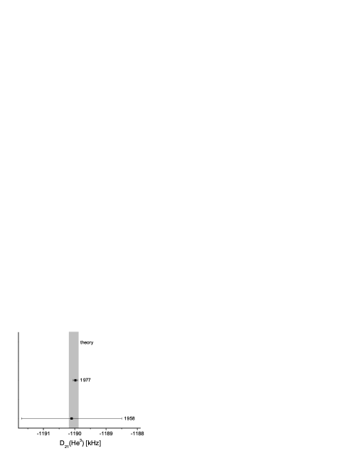
Figure 2: The $D_{21}$ difference for the helium ion ³He⁺: theory versus experiment.

Theory is in perfect agreement with experiment. The most important consequence of our conservative estimation of the theoretical uncertainty is the fact that the experimental result (13) is now twice more accurate than that of the theoretical prediction (12), while previously the relation was opposite.

The procedure presented here has allowed to estimate uncertainty of the extrapolation of the numerical data properly for $D_{21}$. Such an extrapolation occurs for a number of problems in QED theory for hydrogen-like atoms, and a plausible estimation of the accuracy is a crucial issue for the comparison of precision theoretical and experimental results. We hope that an application of our procedure will be helpful for other problems.

The hydrogen and deuterium data will be discussed elsewhere together with experimental progress in the field.

The authors are grateful to S. I. Eidelman for useful discussions. A part of this work was done during a visit of VGI to Garching and he is grateful to MPQ for their hospitality. This work was supported in part by the RFBR grants 03-02-04029 and 03-02-16843 and DFG grant GZ 436 RUS 113/769/0-1.

References

- [1] N. Ramsey, in: Quantum Electrodynamics, ed. by T. Kinoshita (World Scientific, Singapore 1990), p. 673.
- [2] S. G. Karshenboim, in: Precision Physics of Simple Atomic Systems, Ed. by S. G. Karshenboim and V. B. Smirnov, (Springer, Berlin Heidelberg 2001) p. 141.
-
[3]
S.G. Karshenboim and V.G. Ivanov,
Phys. Lett. B 524, 259 (2002);
S.G. Karshenboim and V.G. Ivanov, Euro. Phys. J. D 19, 13 (2002). - [4] S.G. Karshenboim, Int. J. Mod. Phys. A 19, 3879 (2004).
- [5] V. A. Yerokhin and V. M. Shabaev, Phys. Rev. A 64, 012506 (2001).
- [6] D. Zwanziger, Phys. Rev. 121, 1128 (1961).
- [7] P. Mohr, private communication. Quoted according to [10].
- [8] V.G. Ivanov and S.G. Karshenboim, in: Hydrogen atom: Precision physics of simple atomic systems, ed. by S.G. Karshenboim et al (Springer, Berlin, Heidelberg, 2001), pp. 637–650; e-print: hep-ph/0009069.
- [9] H. A. Schluessler, E. N. Forton and H. G. Dehmelt, Phys. Rev. 187, 5 (1969).
- [10] M.H. Prior and E.C. Wang, Phys. Rev. A 16, 6 (1977).
- [11] R. Novick and D. E. Commins, Phys. Rev. 111, 822 (1958).