Heavy Quark Diffusion from the Lattice

Abstract

We study the diffusion of heavy quarks in the Quark Gluon Plasma using the Langevin equations of motion and estimate the contribution of the transport peak to the Euclidean current-current correlator. We show that the Euclidean correlator is remarkably insensitive to the heavy quark diffusion coefficient and give a simple physical interpretation of this result using the free streaming Boltzmann equation. However if the diffusion coefficient is smaller than $\sim 1/(\pi T)$, as favored by RHIC phenomenology, the transport contribution should be visible in the Euclidean correlator. We outline a procedure to isolate this contribution.

I Introduction

The experimental relativistic heavy ion program has produced a variety of evidences which suggest that a Quark Gluon Plasma (QGP) has been formed at the Relativistic Heavy Ion Collider (RHIC) Bellwied:2005kq ; Adcox:2004mh . One of the most exciting results from RHIC so far is the large azimuthal anisotropy of light hadrons with respect to the reaction plane, known as elliptic flow. The observed elliptic flow is significantly larger than was expected from kinetic calculations Molnar:2001ux , but in fairly good agreement with simulations based upon ideal hydrodynamics Ollitrault:1992bk ; Hirano:2004er ; Teaney:2001av ; Kolb:2000fh ; Huovinen:2001cy . This result suggests that the transport mean free path is small enough to employ thermodynamics and hydrodynamics to describe the heavy ion reaction. However, this interpretation of the RHIC results demands further theoretical and experimental corroboration.

Experimentally, this interpretation can be challenged by measuring the elliptic flow of charm and bottom mesons Laue:2004tf ; Adler:2005ab ; Adler:2004ta . The first experimental results show a non-zero elliptic flow for these heavy mesons. Naively, since the quark mass is significantly larger than the temperature of the medium, the relaxation time of heavy mesons is $\sim M/T$ longer than the light hadron relaxation time

$$\tau_{R}^{\rm heavy}\sim\frac{M}{T}\tau_{R}^{\rm light}\,.$$

Consequently the heavy meson elliptic flow should be reduced relative to the light hadrons. Recently, a variety of phenomenological models have estimated how the transport mean free path of heavy quarks in the medium is ultimately reflected in the elliptic flow Moore:2004tg ; Molnar:2004ph ; Zhang:2005ni . The result of these model studies is best expressed in terms of the heavy quark diffusion coefficient. (In a relaxation time approximation the diffusion coefficient is related to the equilibration time, $\tau_{R}^{\rm heavy}=\frac{T}{M}D$.) There is a consensus from the models that if the diffusion coefficient of the heavy quark is greater than

$$D\mbox{~{}{\raisebox{1.72218pt}{$>$}} {\raisebox{-2.58334pt}{$\sim$}}~{}}\frac{1}{T}\,,$$

the heavy quark elliptic flow will be small and probably in contradiction with current data.

Theoretically, transport coefficients have been computed in the perturbative quark gluon plasma using kinetic theory Baymetal ; AMY6 . The heavy quark diffusion coefficient has also been computed Moore:2004tg ; Svetitsky:1987gq ; Braaten:1991we . Recent efforts have also explored some meson resonance models and found a substantially smaller diffusion coefficient than in perturbation theory vanHees:2004gq . The ambiguity in these calculations underscores the need for reliable non-perturbative estimates of transport coefficients in the QGP.

Kubo formulas relate hydrodynamic transport coefficients to the small frequency behavior of real time correlation functions Forster ; BooneYip . Correlation functions in real time are in turn related to correlation functions in imaginary time by analytic continuation. Karsch and Wyld karschwyld first attempted to use this connection to extract the shear viscosity of QCD from the lattice. More recently, additional attempts to extract the shear viscosity nakamura97 ; nakamura05 and electric conductivity gupta03 have been made. We will argue on general grounds that Euclidean correlations functions are remarkably insensitive to transport coefficients. For weakly coupled field theories this has been discussed by Aarts and Resco aarts02 . For this reason, only precise lattice data and a comprehensive understanding of the different contributions to the Euclidean correlator can constrain the transport coefficients.

In this paper we are going to estimate the contribution of heavy quark diffusion to Euclidean vector current correlators. The case of heavy quarks is special since the time scale for diffusion, $M/T^{2}$, is much longer than any other time scale in the problem. In terms of the spectral functions, this separation means that transport processes contribute at small energy, $\omega\sim T^{2}/M$, and all other contributions (e.g. resonances and continuum contributions) start at high energy, $\omega\mbox{~{}{\raisebox{1.72218pt}{$>$}} {\raisebox{-2.58334pt}{$\sim$}}~{}}2M$. For light quarks, transport contributes to meson spectral functions for $\omega\sim g^{4}T$. This scale is separated from the energy scale of other contributions, $\omega\sim T,gT$, only in the weak coupling limit $g\ll 1$.

The behavior of vector current correlators at large times can be related to the heavy quark diffusion constant. Euclidean heavy meson correlators at temperatures above the deconfinement temperature have been calculated on the lattice and attempts to extract spectral functions have been made umeda02 ; asakawa04 ; datta04 . Transport should show up as a peak at very small frequencies, $\omega\simeq 0$. So far, it has not been observed in these studies. Obviously, it is very difficult to reconstruct the spectral functions from the finite temperature lattice correlators, as the time extent is limited by the inverse temperature. However, the temperature dependence of the correlators can be determined to very high accuracy datta04 ; jako05 and therefore some information about the transport can be ascertained.

II Linear Response and the Spectral Density

This section briefly reviews linear response which is the appropriate framework to connect the Langevin and diffusion equations to the current-current correlator Forster . We will also define the spectral density which is needed to relate the Euclidean current-current correlator measured on the lattice to its Minkowski counterpart.

Consider a small perturbing Hamiltonian

$$H=H_{0}-\int d^{3}{\bf x}\,h({\bf x},t)\,O({\bf x},t)\,,$$ (1)

where $h({\bf x},t)$ is a classical source. Now imagine that we slowly turn on the external source $h({\bf x},t)$, and then abruptly turn it off at time $t=0$. $h({\bf x},t)$ obeys

$$h({\bf x},t)=e^{\epsilon t}\theta(-t)\,h^{0}({\bf x})\,.$$ (2)

The expectation value of $\left\langle\delta O({\bf x},t)\right\rangle$ in the presence of the perturbing Hamiltonian is

$$\left\langle\delta O({\bf x},t)\right\rangle=+i\int d^{3}{\bf y}\int_{-\infty}^{t}dt^{\prime}\,\left\langle\left[O({\bf x},t),O({\bf y},t^{\prime})\right]\right\rangle\ h({\bf y},t^{\prime})\,.$$ (3)

Using translational invariance and taking spatial Fourier transforms we have

$$\left\langle\delta O({\bf k},t)\right\rangle=\int_{-\infty}^{+\infty}dt^{\prime}\,\chi({\bf k},t-t^{\prime})\,h({\bf k},t^{\prime})\,,$$ (4)

where

$$\chi({\bf k},t-t^{\prime})=\int d^{3}{\bf x}\>e^{-i{\bf k}\cdot{\bf x}}\,i\theta(t-t^{\prime})\,\left\langle\left[O({\bf x},t),O({\bf y},t^{\prime})\right]\right\rangle\,,$$ (5)

is the retarded correlator. When confusion can not arise we use momentum labels ${\bf p},{\bf k},{\bf q},\dots$ rather than position labels ${\bf x},{\bf y},{\bf z},\dots$ to distinguish the spatial Fourier transform of a field $\left\langle O({\bf k},t)\right\rangle=\int e^{i{\bf k}\cdot{\bf x}}\left\langle O({\bf x},t)\right\rangle$ from the field itself, $\left\langle O({\bf x},t)\right\rangle$.

For $t>0$, differentiating with respect to $t$ we have

$$\frac{\partial}{\partial t}\left\langle\delta O({\bf k},t)\right\rangle=\int_{-\infty}^{+\infty}dt^{\prime}\,\frac{\partial}{\partial t}\chi({\bf k},t-t^{\prime})\,h({\bf k},t^{\prime})\,.$$ (6)

Using $\frac{\partial}{\partial t}\chi({\bf k},t-t^{\prime})=-\frac{\partial}{\partial t^{\prime}}\chi({\bf k},t-t^{\prime})$, integrating by parts with respect to $t^{\prime}$, and using Eq. (2), we find a relation between expectation values and correlators

$$\frac{\partial}{\partial t}\left\langle\delta O({\bf k},t)\right\rangle=-\chi({\bf k},t)h^{0}({\bf k})\,.$$ (7)

The external field $h^{0}({\bf k})$ can be eliminated by using the relation between the static susceptibility $\chi_{s}$, the initial condition $\left\langle\delta O({\bf k},t)\right\rangle$, and the external field

$$\left\langle\delta O({\bf k},t=0)\right\rangle=\chi_{s}({\bf k})\,h^{0}({\bf k})\,,$$ (8)

where the static susceptibility $\chi_{s}({\bf k})$, follows from Eq. (5)

$$\chi_{s}({\bf k})=\int_{0}^{\infty}dt^{\prime}\,e^{-\epsilon t^{\prime}}\,\chi({\bf k},t^{\prime})\,.$$ (9)

Eliminating the field $h^{0}({\bf k})$, we find

$$\chi_{s}({\bf k})\frac{\partial}{\partial t}\left\langle\delta O({\bf k},t)\right\rangle=-\chi({\bf k},t)\,\left\langle\delta O({\bf k},t=0)\right\rangle\,.$$ (10)

This result relates the time evolution of an average from a specified initial condition to an equilibrium correlator $\chi({\bf k},t)$.

The function $\chi({\bf k},t)$ is related to the spectral density. The Fourier transform of the retarded correlator can be written

$$\chi({\bf k},\omega)=\int_{0}^{+\infty}dt\,e^{+i\omega t}\,\chi({\bf k},t)\,.$$ (11)

$\chi({\bf x},t)$ is real, and since the integration is only over positive times, $\chi({\bf k},\omega)$ is analytic in the upper half plane. Provided the Hamiltonian is time-reversal invariant and the operator $O$ has definite signature under time reversal, $\left\langle[O({\bf x},t)\,,O({\bf y},0)]\right\rangle$ is an odd function of time and $\chi({\bf k},t)$ is an even (odd) function of ${\bf k}$ (time). The spectral density, $\rho({\bf k},\omega)$, is defined as the imaginary part by $\pi$ of the retarded correlator

$$\rho({\bf k},\omega)=\frac{{\rm Im}\chi({\bf k},\omega)}{\pi}=\frac{1}{2\pi}\int d^{3}{\bf x}\int_{-\infty}^{\infty}e^{-i{\bf k}\cdot{\bf x}+i\omega t}\left\langle[O({\bf x},t),O(0,0)]\right\rangle\,.$$ (12)

By inserting complete sets of states, one may show that the spectral density is an odd function of frequency and is positive for $\omega>0$ leBellac .

The Euclidean correlator may be deduced from the spectral density. Euclidean tensors are defined from their Minkowski counter parts, $\left.O_{M}^{\mu_{1}\dots\mu_{n}}\right._{\nu_{1}\dots\nu_{n}}(-i\tau)\equiv(-i)^{r}(i)^{s}\left.O_{E}^{\mu_{1}\dots\mu_{n}}\right._{\nu_{1}\dots\nu_{n}}(\tau)$, where $r$ and $s$ are the number of zeros in $\{\mu_{1}\dots\mu_{n}\}$ and $\{\nu_{1}\dots\nu_{n}\}$ respectively. In what follows, we will drop the “$M$” on Minkowski operators but indicate “$E$” on Euclidean operators. With these definitions $x^{0}=-ix^{0}_{E}=-i\tau$, and Euclidean tensors transform under $O(4)$ in the zero temperature limit. Correlators in Euclidean space time are of the following form:

$$G({\bf k},\tau)=\int d^{3}{\bf x}\,e^{i{\bf k}\cdot{\bf x}}\,\left\langle O_{E}({\bf x},\tau)\,O_{E}(0,0)\right\rangle\equiv(-1)^{r+s}\int d^{3}{\bf x}\,e^{i{\bf k}\cdot{\bf x}}\,D^{>}({\bf x},-i\tau)\,,$$ (13)

where $D^{>}({\bf x},t)=\left\langle O({\bf x},t)O(0,0)\right\rangle$ . Usually, the lattice works with at zero spatial momentum ${\bf k}=0$. In Minkowski space, we work with the Fourier transform of $D^{>}({\bf x},t)$,

$$D^{>}({\bf k},\omega)=\int d^{4}x\,e^{+i\omega t-i{\bf k}\cdot{\bf x}}\,D^{>}({\bf x},t)\,.$$ (14)

Similarly, we define $D^{<}({\bf x},t)\equiv\left\langle O(0,0)\,O({\bf x},t)\right\rangle$ and its Fourier transform. Thus, the spectral density, Eq. (12), is given by

$$\rho({\bf k},\omega)=\frac{D^{>}({\bf k},\omega)-D^{<}({\bf k},\omega)}{2\pi}\,.$$ (15)

Using the Kubo-Martin Schwinger (KMS) relation $D^{>}({\bf k},t)=D^{<}({\bf k},t+i/T)$, and its Fourier counter-part $D^{>}({\bf k},\omega)=e^{+\omega/T}D^{<}({\bf k},\omega)$, one discovers the relation between the spectral density and the Euclidean correlator,

$$G({\bf k},\tau)=(-1)^{r+s}\int_{0}^{\infty}d\omega\,\rho({\bf k},\omega)\frac{\cosh\left(\omega\left(\tau-\frac{1}{2T}\right)\right)}{\sinh\left(\frac{\omega}{2T}\right)}\,.$$ (16)

Again, given an operator, $\left.O^{\mu_{1}\dots\mu_{n}}\right._{\nu_{1}\dots\nu_{n}}$,   $r$ and $s$ are the number of zeros in the space-time indices $\{\mu_{1}\dots\mu_{n}\}$ and $\{\nu_{1}\dots\nu_{n}\}$ respectively.

For our discussion two correlators will be important: the density-density correlator

$$D^{>}_{\scriptscriptstyle NN}({\bf x},t)=\left\langle J^{0}({\bf x},t)J^{0}(0,0)\right\rangle\,,$$ (17)

and the current-current correlator

$$D^{>,ij}_{\scriptscriptstyle JJ}({\bf x},t)=\left\langle J^{i}({\bf x},t)J^{j}(0,0)\right\rangle\,.$$ (18)

These correspond to the Euclidean correlators calculated on the lattice

$$G_{\scriptscriptstyle NN}({\bf x},\tau)=\left\langle J^{0}_{E}({\bf x},\tau)J^{0}_{E}(0,0)\right\rangle=-D_{\scriptscriptstyle NN}^{>}({\bf x},-i\tau)\,,$$ (19)

$$G_{\scriptscriptstyle JJ}^{ij}({\bf x},\tau)=\left\langle J^{i}_{E}({\bf x},\tau)J^{j}_{E}(0,0)\right\rangle=D_{\scriptscriptstyle JJ}^{>,ij}({\bf x},-i\tau)\,.$$ (20)

The corresponding retarded correlators $\chi_{\scriptscriptstyle NN}({\bf x},t)$ and $\chi^{ij}_{\scriptscriptstyle JJ}({\bf x},t)$ can be introduced in the same way. The Fourier transforms of current-current correlators can be decomposed into longitudinal and transverse parts. For the retarded correlator we write:

$$\chi_{\scriptscriptstyle JJ}^{ij}({\bf k},\omega)=\left(\frac{k^{i}k^{j}}{k^{2}}-\delta^{ij}\right)\,\chi_{\scriptscriptstyle JJ}^{T}({\bf k},\omega)+\frac{k^{i}\,k^{j}}{k^{2}}\,\chi_{\scriptscriptstyle JJ}^{L}({\bf k},\omega)\,.$$ (21)

Current conservation relates the density-density and the longitudinal current-current correlators

$$\frac{\omega^{2}}{k^{2}}\chi_{\scriptscriptstyle NN}({\bf k},\omega)=\frac{k^{i}k^{j}}{k^{2}}\chi_{\scriptscriptstyle JJ}^{ij}({\bf k},\omega)=\chi_{\scriptscriptstyle JJ}^{L}({\bf k},\omega)\,.$$ (22)

For $k=0$ there is no distinction between the longitudinal and transverse parts and therefore for $k\ll T$ , $\chi_{\scriptscriptstyle JJ}^{L}({\bf k},\omega)\simeq\chi_{\scriptscriptstyle JJ}^{T}({\bf k},\omega)$. Since the transverse component of the current-current correlator is not studied in this work, we will drop the “L”, and for instance, $G_{\scriptscriptstyle JJ}$ and $\rho_{\scriptscriptstyle JJ}$ are short for $G_{\scriptscriptstyle JJ}^{L}$ and $\rho_{\scriptscriptstyle JJ}^{L}$.

At finite temperature the spectral function can be written as

$$\rho_{\scriptscriptstyle JJ}({\bf k},\omega)=\rho_{\scriptscriptstyle JJ}^{\rm low}({\bf k},\omega)+\rho_{\scriptscriptstyle JJ}^{\rm high}({\bf k},\omega)\,,$$ (23)

where the last term is just the zero temperature part and the first term is the low energy $\omega\ll T^{2}/M$ contribution. In the next two sections we will discuss how to estimate the low frequency part.

III Transport in Euclidean Correlators

In this section we estimate how the low frequency part of the spectral function contributes to the Euclidean current-current correlator. To leading order, the moments of the spectral function, the time derivatives of the retarded correlator at $t=0$, and the derivatives of the Euclidean correlator at $\beta/2$, are in one-to-one correspondence. Since the leading contribution is due to time derivatives at $t=0$, the free streaming of heavy quarks gives the dominant contribution to the Euclidean current-current correlator. The first scattering correction appears in the second (fourth) derivative at $\beta/2$ of the current-current (density-density) euclidean correlator.

First let us start with the density-density correlator. For small frequencies, the kernel in Eq. (16) is given by $2T/\omega$, and thus we can write

$$-G_{\scriptscriptstyle NN}^{\rm low}({\bf k},\tau)\simeq 2T\,\int_{0}^{\infty}\frac{d\omega}{\omega}\,\rho_{\scriptscriptstyle NN}^{\rm low}({\bf k},\omega)\,.$$ (24)

Inserting the definition of the spectral density

$$\rho_{\scriptscriptstyle NN}^{\rm low}({\bf k},\omega)=\frac{1}{\pi}\int_{0}^{\infty}dt\,\sin(\omega t)\,\chi_{\scriptscriptstyle NN}({\bf k},t)\,,$$ (25)

and performing the integral over frequency, we find

$$-G_{\scriptscriptstyle NN}^{\rm low}({\bf k},\tau)\simeq\int_{0}^{\infty}dt\,\chi_{\scriptscriptstyle NN}^{\rm low}({\bf k},t)=T\chi_{s}({\bf k})\,.$$ (26)

The last equality follows from Eq. (9). Similarly, the low energy contribution to the longitudinal current correlator is

$$G_{\scriptscriptstyle JJ}^{\rm low}({\bf k},\tau)\simeq 2T\int_{0}^{\infty}\frac{d\omega}{\omega}\,\rho_{\scriptscriptstyle JJ}^{\rm low}({\bf k},\omega)\,\left[1-\frac{1}{6}\left(\frac{\omega}{2T}\right)^{2}+\omega^{2}\,\frac{1}{2}\left(\tau-\beta/2\right)^{2}+\dots\right]\,.$$ (27)

Inserting the spectral density

$$\rho_{\scriptscriptstyle JJ}^{\rm low}({\bf k},\omega)=\frac{\omega^{2}}{\pi\,k^{2}}\int_{0}^{\infty}dt\,\sin(\omega t)\,\chi_{\scriptscriptstyle NN}({\bf k},t)\,,$$ (28)

and performing the integral over frequency, we find

$$G_{\scriptscriptstyle JJ}^{\rm low}({\bf k},\tau)=\frac{T}{k^{2}}\left[\partial_{t}^{(1)}\chi_{\scriptscriptstyle NN}({\bf k},t)+\frac{1}{24\,T^{2}}\partial_{t}^{(3)}\chi_{\scriptscriptstyle NN}({\bf k},t)\,-\,\partial_{t}^{(3)}\chi_{\scriptscriptstyle NN}({\bf k},t)\,\frac{1}{2}\left(\tau-\beta/2\right)^{2}+\dots\right]_{t=0}\,.$$ (29)

Thus we see that the dominant low energy contributions to the Euclidean correlator is given by the short time behavior of the retarded correlator. Indeed, as seen from Eq. (27) and Eq. (29), the moments of the spectral function, the $\tau$ derivatives of the Euclidean correlator at $\beta/2$, and the time derivatives of the real-time retarded correlator at $t=0$ are in one to one correspondence. While a short time expansion can never be used to rigorously extract transport coefficients, they have proved useful in in non-relativistic contexts Forster ; BooneYip

For times which are short compared to the collision time it is reasonable to expect that the motion of heavy quarks is described by the free-streaming Boltzmann equation. Even in the interacting theory, the free streaming Boltzmann equation will describe the first time derivative of the retarded correlator or the first term in the Euclidean correlator, Eq. (29).

Let us create an excess of heavy quarks, and subsequently study the diffusion of this excess at short times. This can be done by introducing a small chemical potential $\mu({\bf x})=\mu_{0}+\delta\mu({\bf x})$ as in Section II. Then the thermal distribution function at an initial time $t=0$ is

$$f_{0}({\bf x},{\bf p})\equiv\frac{1}{e^{(E_{p}-\mu({\bf x}))/T}\mp 1}\approx f_{p}+f_{p}\,(1\pm f_{p})\,\frac{\delta\mu({\bf x})}{T}\,,$$ (30)

with,  $f_{p}=1/(e^{(E_{p}-\mu_{0})/T}\mp 1)$ . For short times the collision-less Boltzmann equation applies,

$$\left[\frac{\partial}{\partial t}+v_{\bf p}^{i}\frac{\partial}{\partial x^{i}}\right]f({\bf x},{\bf p},t)=0\,.$$ (31)

The solution to this equation with the specified initial conditions is

$$f({\bf x},{\bf p},t)=f_{0}({\bf x}-v_{\bf p}t,{\bf p})\,.$$ (32)

Then the fluctuation in the number density is

$$\delta N({\bf x},t)=\int\frac{d^{3}{\bf p}}{(2\pi)^{3}}\>\,\delta f({\bf x},{\bf p},t)\,,$$ (33)

with $\delta f({\bf x},{\bf p},t)=f({\bf x},{\bf p},t)-f_{p}$ . Then taking spatial Fourier transforms with ${\bf k}$ conjugate to ${\bf x}$ and substituting the distribution function, Eq. (32), we have

$$\delta N({\bf k},t)=\left[\frac{1}{T}\int\frac{d^{3}{\bf p}}{(2\pi)^{3}}\>e^{-i{\bf k}\cdot v_{\bf p}t}f_{p}(1\pm f_{p})\right]\delta\mu({\bf k})\,.$$ (34)

For small times, we expand the exponential, and find

$$\delta N({\bf k},t)=\left[\chi_{s}({\bf k})-\frac{1}{2}\,t^{2}\,k^{2}\,\chi_{s}({\bf k})\left\langle\frac{v^{2}}{3}\right\rangle\right]\delta\mu({\bf k})\,,$$ (35)

with

$$\chi_{s}({\bf k})=\frac{\partial N}{\partial\mu_{0}}=\frac{1}{T}\int\frac{d^{3}{\bf p}}{(2\pi)^{3}}\>f_{p}(1\pm f_{p})\,,$$ (36)

and

$$\left\langle\frac{v^{2}}{3}\right\rangle=\frac{1}{T\chi_{s}({\bf k})}\,\int\frac{d^{3}{\bf p}}{(2\pi)^{3}}\>f_{p}(1\pm f_{p})\,\frac{v_{\bf p}^{2}}{3}\,.$$ (37)

Thus, from Eq. (29), Eq. (7), and Eq. (35), we find

$$G_{\scriptscriptstyle JJ}^{L,\,\rm low}({\bf k},\tau)=T\chi_{s}({\bf k})\,\left\langle\frac{v^{2}}{3}\right\rangle\,.$$ (38)

In the free theory, at ${\bf k}=0$ there there are no corrections to this result and the Euclidean correlator is a constant. At finite ${\bf k}$, the lattice correlator is not a constant even in the free theory. For massless particles, $\left\langle v^{2}/3\right\rangle=1/3$, while for massive we have $\left\langle v^{2}/3\right\rangle=T/M$.

We have outlined the short time expansion of $\chi_{\scriptscriptstyle NN}({\bf k},t)$ . Further insight is gained from the full free spectral function. From, Eq. (34), Eq. (7) and a simple Fourier transform we deduce that the retarded correlator from the free streaming Boltzmann equation is

$$\chi_{\scriptscriptstyle NN}({\bf k},\omega)=\frac{1}{T}\int\frac{d^{3}{\bf p}}{(2\pi)^{3}}\>f_{p}(1\pm f_{p})\,\frac{-{\bf k}\cdot{\bf v}_{\bf p}}{\omega-{\bf k}\cdot{\bf v}_{\bf p}+i\epsilon}\,.$$

Taking the imaginary part, the corresponding spectral density is

$$\rho_{\scriptscriptstyle NN}^{\rm low}({\bf k},\omega)=\frac{1}{T}\int\frac{d^{3}{\bf p}}{(2\pi)^{3}}\>f_{p}(1\pm f_{p})\,{\bf k}\cdot{\bf v}_{\bf p}\,\delta(\omega-{\bf k}\cdot{\bf v}_{\bf p})\,.$$

As shown in Appendix B, this form for the spectral density is identical to the one loop spectral function of the free theory at small $k$ and $\omega$, Eq. (79). As discussed in Appendix B, the resulting integral can be performed in the non-relativistic limit and we find the free spectral function for the heavy quark current-current correlator

$$\rho_{\scriptscriptstyle JJ}^{\rm low}({\bf k},\omega)=\chi_{s}\,\frac{\omega^{3}}{k^{2}}\frac{1}{\sqrt{2\pi k^{2}\left\langle\frac{v^{2}}{3}\right\rangle}}\exp\left(-\frac{\omega^{2}}{2k^{2}\left\langle\frac{v^{2}}{3}\right\rangle}\right)\,.$$ (39)

This is the dynamic structure factor of a free non-relativistic gas BooneYip . In the free theory, the spectral function is essentially a Gaussian, with a width that is proportional to $k^{2}$. In the limit that ${\bf k}=0$ the correlator is

$$\rho_{\scriptscriptstyle JJ}^{L,\rm low}({\bf k},\omega)=\chi_{s}\left\langle\frac{v^{2}}{3}\right\rangle\,\omega\delta(\omega)\,.$$ (40)

In the free theory, the low frequency spectral density is infinitely narrow at ${\bf k}=0$. The moments of the spectral density are in one to one correspondence with the derivatives of the Euclidean correlator at $\beta/2$. Since higher moments of a delta function are zero, all derivatives at $\beta/2$ vanish and the low frequency contribution of the free theory to the Euclidean correlator is simply a flat line. Thus, provided the high frequency contribution of the spectral function can be subtracted, any bending of the Euclidean correlator is indicative of something beyond free streaming. In the next sections we will discuss how interactions smear the $\delta(\omega)$ function and estimate how much the Euclidean correlator curves at $\beta/2$ as a function of diffusion coefficient.

IV Heavy Quark Diffusion in the Langevin Effective Theory

In this section we will discuss the predictions of the Langevin equations for the retarded correlator. As mentioned before, the time scale for heavy quark transport, $M/T^{2}$ is much larger than typical time scale for light degrees of freedom in the plasma. For this reason we will assume that the Langevin equations provide a good macroscopic description of the thermalization of charm quarks Moore:2004tg ,

$$\frac{dx^{i}}{dt} = \frac{p^{i}}{M}\,,$$

$$\frac{dp^{i}}{dt} = \xi^{i}(t)-\eta p^{i}\,,\qquad\langle\xi^{i}(t)\xi^{j}(t^{\prime})\rangle=\kappa\delta^{ij}\delta(t-t^{\prime})\,.$$

The drag and fluctuation coefficients are related by the fluctuation dissipation relation

$$\eta=\frac{\kappa}{2MT}\,.$$ (41)

For timescales which are much larger than $1/\eta$ the heavy quark number density obeys ordinary diffusion equation

$$\partial_{t}N+D\nabla^{2}N=0\,.$$

The drag coefficient $\eta$ can be related to the diffusion coefficient through the Einstein relation

$$D=\frac{T}{M\eta}=\frac{2T^{2}}{\kappa}\,.$$ (42)

The effective Langevin theory can be derived from kinetic theory in the weak coupling limit Moore:2004tg and probably is adequate for describing heavy quark diffusion even for strongly interacting plasma. The Langevin equations make a definite prediction for the retarded correlator. Following the framework of linear response, consider an initial distribution of heavy quarks when a small perturbing chemical potential is applied, $\mu({\bf x})=\mu_{0}+\delta\mu({\bf x})$. The initial phase space distribution of heavy quarks is

$$f({\bf x},{\bf p},t=0)=e^{\frac{\mu({\bf x})}{T}-\frac{M}{T}}e^{-\frac{p^{2}}{2MT}}\,.$$ (43)

Summing over spins and colors, the initial number density of quarks minus anti-quarks is

$$N({\bf x},t=0)=\left[4N_{c}\right]\,\left(\frac{M\,T}{2\pi}\right)^{3/2}\,e^{-\frac{M}{T}}\,\sinh\left(\frac{\mu({\bf x})}{T}\right)\,.$$ (44)

By comparing Eq. (44) and Eq. (8), we find the static susceptibility

$$\chi_{s}=[4N_{c}]\,\left(\frac{M\,T}{2\pi}\right)^{3/2}\,e^{-\frac{M}{T}}\,\cosh\left(\frac{\mu_{0}}{T}\right)\,.$$ (45)

Let $P({\bf x},t)$ be the probability that a heavy quark starts at the origin at $t=0$ and moves a distance ${\bf x}$ over a time $t$ . Consider the relaxation of an initial distribution of heavy quarks $N({\bf x},t=0)$ slightly perturbed from equilibrium. The distribution of heavy quarks at a later time is,

$$N({\bf x},t)=\int\,d^{3}{\bf x}^{\prime}\,P({\bf x}-{\bf x}^{\prime},t)\,N({\bf x}^{\prime},0)\,,$$ (46)

or

$$N({\bf k},t)=P({\bf k},t)N({\bf k},0)\,.$$ (47)

Comparing this result with the linear response result, Eq. (10), we conclude that for small ${\bf k}$ and times large compared to typical medium timescale

$$\chi_{\scriptscriptstyle NN}({\bf k},t)=-\chi_{s}({\bf k})\,\partial_{t}P({\bf k},t)\,.$$ (48)

Thus, to find the retarded correlator $\chi_{\scriptscriptstyle NN}({\bf k},\omega)$ , we need only find the probability $P({\bf x},t)$.

The probability distribution $P({\bf x},t)$ is determined in Appendix A. Not surprisingly, the distribution is a Gaussian,

$$P({\bf x},t)=\frac{1}{(2\pi\sigma^{2}(t))^{3/2}}\exp\left(-\frac{1}{2}\frac{x^{2}}{\sigma^{2}(t)}\right)\,,$$ (49)

with a width that depends non-trivially on time

$$\sigma^{2}(t)=2Dt-\frac{2D}{\eta}(1-e^{-\eta t})\,.$$ (50)

For large times, we have $\sigma^{2}(t)\approx 2D\,t$ as expected from the ordinary diffusion equation. For small times, we have

$$\sigma^{2}(t)\approx(T/M)\,t^{2}\qquad\qquad(\eta t\ll 1)\,,$$ (51)

which reflects the initial thermal velocity distribution of heavy quarks, $\left\langle v^{2}/3\right\rangle=T/M$. Using Eq. (48), the probability distribution Eq. (49), and the definition of the retarded correlator, we find the following form:

$$\chi_{\scriptscriptstyle NN}({\bf k},\omega)=\chi_{s}({\bf k})\,\int_{0}^{\infty}dt\,e^{i\omega t}\,k^{2}D\,(1-e^{-\eta\,t})\,e^{-k^{2}Dt\ +\ (k^{2}D/\eta)\,(1-e^{-\eta\,t})}\,.$$ (52)

Eq. (52) summarizes the contribution of the Langevin equations to the retarded density-density correlator. The retarded correlator has following properties:

• For small ${\bf k}$, $Dk^{2}\ll\eta$, and arbitrarily large times, we may write the integrand as $k^{2}D\,(e^{-k^{2}Dt}-e^{-\eta\,t})$, and perform the integration

  $$\chi_{\scriptscriptstyle NN}({\bf k},\omega)=\frac{\chi_{s}({\bf k})\,Dk^{2}}{-i\omega+k^{2}D}-\frac{\chi_{s}({\bf k})\,Dk^{2}}{-i\omega+\eta}\,.$$ (53)

  For small frequency $\omega\sim Dk^{2}$, the first term dominates and recalls the diffusion equation, $(\partial_{t}+D\nabla^{2})^{-1}$. For large frequencies $\omega\sim\eta$, $\chi_{NN}$ recalls the drag term of the Langevin equations, $(\partial_{t}+\eta)^{-1}$ . Of particular relevance to lattice measurements is the spectral density of the current-current correlator at ${\bf k}=0$

  $$\frac{\rho_{\scriptscriptstyle JJ}(0,\omega)}{\omega}\equiv\frac{1}{\pi}\,\frac{\mbox{Im}\,\chi_{\scriptscriptstyle JJ}(0,\omega)}{\omega}=\chi_{s}\,\frac{T}{M}\frac{1}{\pi}\,\frac{\eta}{\omega^{2}+\eta^{2}}\,,$$ (54)

• The typical relaxation time of a heavy quark is set by the inverse drag coefficient, $1/\eta=D\,(M/T)$. The typical distance that a heavy quark moves over the relaxation is $\sqrt{T/M}/\eta=D\sqrt{M/T}$. The correlator $\chi_{\scriptscriptstyle NN}$ is a function of a scaled spatial momentum $\bar{k}={\bf k}D\sqrt{M/T}$ and a scaled frequency $\bar{\omega}=\omega D\,(M/T)$. In Fig. 1 we show the spectral weight of the current-current correlator. For comparison we also show the free current-current correlator from Eq. (39).

  

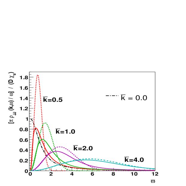
  Figure 1: The spectral density of the longitudinal current-current correlator $\pi\rho_{\scriptscriptstyle JJ}({\bf k},\omega)/\omega$ divided by $D\chi_{s}({\bf k})$ as a function of a scaled frequency $\bar{\omega}\equiv\omega D\,(M/T)$ for various values of a scaled momentum $\bar{{\bf k}}\equiv{\bf k}D\sqrt{M/T}$. The solid lines show the spectral density from the Langevin equations for non-zero $\bar{{\bf k}}$. For comparison, the dotted lines show the spectral function of the free theory, Eq. (39), expressed in the same $\bar{{\bf k}}$ and $\bar{\omega}$ of the interacting theory. The dash-dotted line shows the ${\bf k}=0$ result of the Langevin equations, Eq. (54).

• Noting that $\chi_{\scriptscriptstyle NN}({\bf k},\omega)=-\int_{0}^{\infty}e^{i\omega t}\chi_{s}\partial_{t}P({\bf k},t)$ with $P({\bf k},t)=e^{-k^{2}\sigma^{2}(t)/2}$, it is easy to verify the consistency relation $\chi({\bf k},0)=\chi_{s}({\bf k})$.

V Numerical Estimate of the Euclidean Correlator

In this section we will give a numerical estimate of the Euclidean vector current correlator. We will parametrize the spectral density with low and high frequency contributions.

$$\rho_{\scriptscriptstyle JJ}({\bf k},\omega)=\rho_{\scriptscriptstyle JJ}^{\rm low}({\bf k},\omega)+\rho_{\scriptscriptstyle JJ}^{\rm high}({\bf k},\omega)\,.$$ (55)

The high frequency part is present at zero temperature and will be parametrized as a $J/\psi$ resonance plus a continuum

$$\rho_{\scriptscriptstyle JJ}^{\rm high}({\bf k}=0,\omega)=M_{\scriptscriptstyle J/\psi}^{2}f_{\scriptscriptstyle V}^{2}\,\delta(\omega^{2}-M_{\scriptscriptstyle J/\psi}^{2})+\frac{N_{c}}{8\pi^{2}}\,\theta(\omega^{2}-4M_{D}^{2})\,\omega^{2}\sqrt{1-\frac{4M_{D}^{2}}{\omega^{2}}}\,\left(\frac{2}{3}+\frac{4M_{D}^{2}}{3\omega^{2}}\right)\,.$$ (56)

Here $f_{\scriptscriptstyle V}$ is the $J/\psi$ coupling to dileptons as described in Appendix C. The continuum contribution is motivated by the free spectral function calculated in Appendix B, but we have replaced $2M$ with the open charm threshold $2M_{D}$.

For the low frequency part of the spectral function we will take two functional forms. The first form is the Lorentzian from the Langevin equations

$$\frac{\rho_{\scriptscriptstyle JJ}({\bf k}=0,\omega)}{\omega}=\chi_{s}\,\frac{T}{M}\frac{1}{\pi}\,\frac{\eta}{\omega^{2}+\eta^{2}}\,,$$ (57)

where $\eta=\frac{T}{MD}$. This form is rigorously true when $\frac{T}{MD}\ll T$, and the frequency small $\omega\mbox{~{}{\raisebox{1.72218pt}{$<$}} {\raisebox{-2.58334pt}{$\sim$}}~{}}\eta\ll T$.

These inequalities are strained in our numerical work. For instance, for $T/M_{c}\approx 1/5$ and $D\sim 0.25/T$, $\frac{T}{MD}$, is not really much less than $T$. Further, as discussed in Section III, the transport contribution is dominated by the second moment of the spectral function

$$\int\frac{d\omega}{\omega}\,\rho_{JJ}(\omega)\,\omega^{2}\,.$$ (58)

For the Lorentzian, this moment diverges and the transport contribution to the correlator is sensitive to the high frequency behavior of the ansatz where the Langevin approach is not valid. The higher moments open up the white noise in the Langevin equations. We therefore considered a Gaussian ansatz which falls much more rapidly at infinity

$$\frac{\rho_{{\scriptscriptstyle JJ}}(\omega)}{\omega}=\chi_{s}\frac{T}{M}\,\frac{1}{\sqrt{2\pi\eta^{2}_{\scriptscriptstyle G}}}e^{-\frac{\omega^{2}}{2\,\eta^{2}_{\scriptscriptstyle G}}}\,.$$ (59)

The parameter, $\eta_{\scriptscriptstyle G}=\sqrt{\frac{\pi}{2}}\frac{T}{MD}$, is fixed from the relation between the spectral density and the diffusion coefficient coefficient, $\left.\frac{\rho(\omega)}{\omega}\right|_{\omega=0}=\frac{\chi_{s}D}{\pi}$. The integral under this smeared delta function is again $\chi_{s}\,T/M$. By comparing these functional forms we obtain a feeling for the uncertainties our the estimate.

The temperature dependence of the Euclidean correlators comes from two sources: the temperature dependence of the spectral function $\rho({\bf k},\omega,T)$, and the trivial temperature dependence of the integration kernel, Eq. (16). We obviously want to separate the interesting temperature dependence coming from the spectral function from the trivial temperature dependence coming from the integration kernel. This can be done by defining the reconstructed correlator datta04 .

$$G^{{\rm rec}}_{JJ}({\bf k},\tau,T)=\int_{0}^{\infty}d\omega\,\rho_{JJ}({\bf k},\omega,T=0)\,\frac{\cosh(\omega(\tau-1/(2T)))}{\sinh(\omega/(2T))}\,.$$ (60)

If the spectral function does not change above the deconfinement temperature $T_{c}$, the ratio $G_{JJ}({\bf k},\tau,T)/G_{JJ}^{{\rm rec}}({\bf k},\tau,T)$ should be unity.

First we estimate the relative importance of the transport contribution to the correlator. For closer comparison with existing lattice data, we consider the diffusion of heavy quarks in a gluonic plasma where the transition temperature is $T_{c}=270\,\mbox{MeV}$ edwinowe . At this stage we can set the $\eta$ to zero ($D=\infty$) and consider only the free spectral function. The charm quark mass $M_{c}$ is taken to be $1.3$ GeV. In accord with lattice data umeda02 ; asakawa04 ; datta04 , we will assume that $J/\psi$ is not modified by the medium and determine $f_{\scriptscriptstyle V}$ from its dilepton width (see Appendix C). $M_{\scriptscriptstyle J/\psi}$ and $M_{D}$ are taken from the Particle Data Book pdg In Fig. 2 we show $G_{JJ}({\bf k},\tau,T)/G_{JJ}^{{\rm rec}}({\bf k},\tau,T)$ for several temperatures. The transport contribution is of order $7-12\%$ and is the the only source of the temperature dependence seen in Fig. 2.

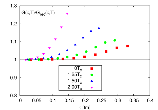
Figure 2: The ratio $G_{JJ}(\tau,T)/G_{JJ}^{\rm rec}(\tau,T)$ for different temperatures and ${\bf k}=0$.

A similar enhancement was found in actual lattice calculations dattasewm04 .

Analytic understanding can be gained by performing the integral over the kernel at $\tau=1/(2T)$. In the heavy quark limit, we set $M_{\scriptscriptstyle J/\psi}\approx 2M$ and $M_{D}\approx M$, and find

$$\left.G_{JJ}({\bf k}=0,\tau,T)\right|_{\tau=\beta/2}=\underbrace{4N_{c}\left(\frac{MT}{2\pi}\right)^{3/2}e^{-\frac{M}{T}}\frac{T}{M}}_{\rm transport}\;+\;\underbrace{M^{3}\left(\frac{f_{\scriptscriptstyle V}}{2M}\right)^{2}\,8\,e^{-\frac{M}{T}}}_{\rm resonance}\;+\;$$

$$\underbrace{4N_{c}\left(\frac{M\,T}{2\pi}\right)^{3/2}e^{-\frac{M}{T}}\left(1-\frac{T}{M}\right)}_{\rm continuum}\,.$$

$f_{\scriptscriptstyle V}/2M\approx 0.131$ is small and suppresses the resonance contribution. The transport contribution is smaller by a factor of $T/M$ relative to the continuum contribution.

Interactions will modify the correlator by only a few percent. These small changes due to the transport must be disentangled from other in-medium effects such as a small shift in the mass or width of the resonance. This can be done by introducing a small chemical potential for the heavy quark, $\mu_{c}\ll M$. Since the transport contribution is proportional to $\chi_{s}$, the small chemical potential will enhance the transport by factor of $\cosh(\mu_{c}/T)$, see Eq. (45). The small charm chemical potential will not affect the resonance and continuum contributions to the spectral function to leading order in the heavy quark density, $\sim e^{-(M-\mu_{c})/T}$. Thus we expect that

$$\delta G_{JJ} \equiv G_{JJ}(\tau,T,\mu)-G_{JJ}(\tau,T,0)$$ (61)

$$\simeq (\cosh(\mu_{c}/T)-1)\int_{0}^{\infty}d\omega\left.\rho_{JJ}^{\rm low}\right|_{\mu=0}(\omega)\frac{\cosh(\omega(\tau-1/(2T)))}{\sinh(\omega/(2T))},$$ (62)

is largely insensitive to the high frequency behavior of the spectral function. For a thousand gauge configurations, the statistical error in the vector current correlators can be reduced below, $0.5\%$. One may hope that the same holds for the difference of the correlators, $\delta G_{JJ}$. Clearly, to achieve this precision one should difference the two correlators before averaging over gauge configurations. This needs to studied with numerical experiments.

In Fig. 3(a) and (b) we show this difference for $T=1.1T_{c}$, $\mu_{c}=M/5$ and

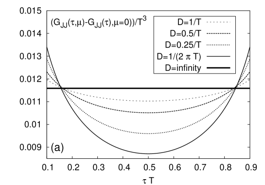
Figure 3: The difference of correlators at $\mu_{c}=M_{c}/5$ and $\mu=0$ for the (a) Lorentzian and (b) Gaussian ansätze and various values of the diffusion coefficient, D.

different values of the diffusion constant $D$. As seen in Fig. 3, and as expected from Eq. (29), the effect of the diffusion coefficient is to provide a small curvature to the correlator and to shift the value of the correlator downward at $\tau=\beta/2$.

First we will concentrate on the curvature. If the final precision is 0.5% and $D\mbox{~{}{\raisebox{1.72218pt}{$<$}} {\raisebox{-2.58334pt}{$\sim$}}~{}}1/(\pi T)$, then from Fig. 3(a), one could hope that the curvature is large enough to be determined in lattice simulations. In practice, it will be difficult to guarantee that the continuum contribution will not affect the extracted value.

The downward shift of the correlator at $\beta/2$ from the constant value, $\chi_{s}T/M$, is a much larger effect. To isolate this transport contribution we consider the difference, $\delta G_{JJ}(M)$, as a function of the heavy quark mass. We plot the ratio

$$R(M)\equiv\left.\frac{\delta G_{JJ}(M)/(\chi_{s}(M)T/M)}{\delta G_{JJ}(M_{0})/(\chi_{s}(M_{0})T/M_{0})}\right|_{\tau=\beta/2}\,.$$ (63)

For the free theory this quantity is one and is independent of the heavy quark mass. Deviations from one are a signature of interactions. Fig. 4(a) and (b) show this ratio as a function of the heavy quark mass for the Lorentzian and Gaussian ansätze.

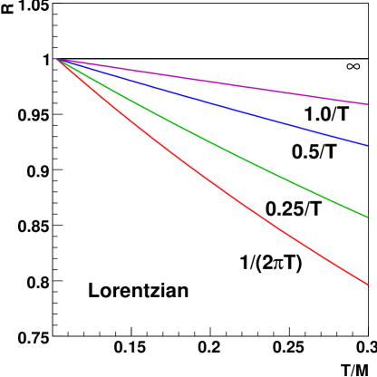
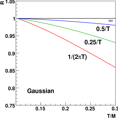
Figure 4: The relative transport contribution to the correlator as a function of quark mass, Eq. (63), for the (a) Lorentzian and (b) Gaussian ansätze to the low frequency spectral function. The numbers indicate the diffusion coefficient for each ansatz.

Examining Fig. 4, we conclude that if the diffusion coefficient is sufficiently small, $D\mbox{~{}{\raisebox{1.72218pt}{$<$}} {\raisebox{-2.58334pt}{$\sim$}}~{}}1/(\pi T)$, the transport peak should be visible in the mass dependence of the Euclidean correlator. Additional critical remarks are left to the conclusions.

VI Brief Summary and Discussion

The Euclidean current-current correlator is remarkably insensitive to the heavy quark diffusion coefficient. Indeed, to leading order in $T/M$, the Euclidean current-current correlator is independent of the diffusion coefficient. This is explained as follows (see Section III). The $\tau$ derivatives of the euclidean current-current correlator at $\tau=\beta/2$, the moments of the spectral function, and time derivatives the real-time retarded correlator at $t=0$, are in one to one correspondence. Thus, the value of the current-current correlator (i.e. the zero-th derivative) is determined only by short times and may be calculated with the free streaming Boltzmann equation. In the end, the value of the current-current correlator at $\beta/2$ is simply $\chi_{s}T/M$, where $\chi_{s}$ is the static susceptibility and $T/M$ reflects average thermal velocity squared. Higher $\tau$ derivatives (or moments of the spectral density) reflect the width of the transport peak and contain useful information about the transport time scales.

In a free theory, the spectral density is proportional to a delta function

$$\frac{\rho_{JJ}({\bf k}=0,\omega)}{\omega}=\chi_{s}\frac{T}{M}\delta(\omega)\,,$$

which reflects the fact that in the free case, the spatial current is conserved in addition to the charge. This result may be found either by using the free streaming Boltzmann equation (see Section III) or performing a one loop expansion (see Appendix B). Since the spectral density is proportional to a delta function, higher $\tau$ derivatives, or moments of the spectral function, vanish and the Euclidean current-current correlator is a constant, independent of $\tau$ (see also Ref. aarts02 ). In the interacting theory the delta function is smeared. Using the Langevin equations of motion, we analyze in Section IV how this delta function is smeared as a function of ${\bf k}$ and $\omega$. This result together with the free theory is summarized in Fig. 1. At ${\bf k}=0$, the Langevin effective theory dictates the replacement

$$\delta(\omega)\rightarrow\frac{1}{\pi}\frac{\eta}{\omega^{2}+\eta^{2}}\,,$$

where $\eta=T/(MD)$ and $D$ is the diffusion coefficient of the heavy quark.

With this Lorentzian form for the spectral function at small omega, we adopted a simple transport + resonance + continuum model for the full spectral function and studied how the Euclidean correlator is modified by the transport peak in Section V. We also smeared the delta function with a Gaussian to illuminate the sensitivity to the Lorentzian ansatz which is only valid in a heavy quark limit and for $\omega\mbox{~{}{\raisebox{1.72218pt}{$<$}} {\raisebox{-2.58334pt}{$\sim$}}~{}}T/(MD)$.

Generally, the transport contribution to the full correlator is suppressed by a factor of $T/M$ relative to the continuum contribution (see Eq. (V)). To disentangle the transport from the continuum and resonance contributions we proposed differencing two current-current correlators – one at finite heavy quark chemical potential and one at zero chemical potential, $\delta G_{JJ}(\tau)\equiv G_{JJ}(\tau,\mu)-G_{JJ}(\tau,0)$ . This difference is proportional to the low frequency contribution and is independent of the high frequency contribution to leading order the heavy quark density, $\sim e^{-(M-\mu)/T}$. With this procedure, the transport contribution can be separated from the other contributions at least parametrically. In practice (as opposed parametrics) our numerical work in Section V shows that extracting this piece is difficult though not impossible. A major unknown is the final precision when the difference of correlators is calculated. Clearly, one should difference and then average over gauge configurations. Exploratory lattice studies are needed to estimate this precision.

The transport contribution to the correlator is displayed separately in Fig. 3(a) and (b) as a function of the diffusion coefficient. As analyzed in Section III, the effect of the diffusion coefficient is to shift the value of the current-current correlator down from its free value $\chi_{s}T/M$, and to curve the correlator at $\beta/2$. Parametrically, these effects are suppressed by $(T/MD)^{2}$ relative to $\chi_{s}T/M$. The figure illustrates that if the diffusion coefficient is much greater than $1/T$ it will be difficult to measure the second derivative at $\beta/2$. However if the precision is $0.5\%$ it may be possible, although it will be hard to guarantee that the continuum contribution has been completely subtracted. To eliminate the continuum contribution it is desirable to make the mass as large as possible. On the other hand, the transport signal is proportional to $(T/MD)^{2}$ and therefore is suppressed by the mass. Ultimately, numerical experiments will determine the optimal heavy quark mass.

Even with these complications, Fig. 3 shows that the Euclidean correlator at $\beta/2$ is clearly shifted downward from its free value, $\chi_{s}\,T/M$. This shift also is indicative of the width of the transport peak. To evaluate the magnitude of this shift, we proposed measuring

$$\left.\delta G_{JJ}(M)/(\chi_{s}(M)\,T/M)\right|_{\tau=\beta/2}\,,$$

as a function of quark mass; this quantity is independent of the mass in the free theory. As is shown in Fig. 4(a) and (b), in the interacting theory the width of the transport peak makes this quantity mass dependent. Judging from Fig. 4, if the diffusion coefficient is less than $\mbox{~{}{\raisebox{1.72218pt}{$<$}} {\raisebox{-2.58334pt}{$\sim$}}~{}}0.25/T$ the effects of the transport peak should be visible in this mass dependence.

Measuring Fig. 3 and Fig. 4 on the lattice is very difficult. The importance of such measurements should spur effort. Only measurements of this kind can seriously challenge the strong coupling assumptions that underly the hydrodynamic interpretation of the RHIC results.

Acknowledgments. We thank Guy D. Moore for useful discussions. D. Teaney was supported by grants from the U.S. Department of Energy, DE-FG02-88ER40388 and DE-FG03-97ER4014. P. Petreczky was also supported by the U.S. Department of Energy, DE-AC02-98CH1086. He is a Goldhaber and RIKEN-BNL fellow.

Appendix A Diffusion of a Brownian Particle

The goal of this appendix is to determine the probability $P({\bf x},t)$ that a Brownian particle will move a distance ${\bf x}$ from the origin over a time $t$. Consider the discretized Langevin equations:

$${\bf x}_{t+1}-{\bf x}_{t} = \frac{{\bf p}_{t}}{M}\,,$$ (64)

$${\bf p}_{t+1}-{\bf p}_{t} = -\eta{\bf p}_{t}\,\Delta t+{\bf\xi}_{t}\,,\qquad\left\langle\xi_{t}^{i}\xi_{t^{\prime}}^{j}\right\rangle=\frac{\kappa}{\Delta t}\delta^{ij}\delta_{tt^{\prime}}\,,$$ (65)

where the noise is drawn from a Gaussian distribution with the specified variance.

Let $W[{\bf p}_{0},{\bf p}_{1},\dots,{\bf p}_{n}]$ be the probability of having a sequence of momenta, ${\bf p}_{0},{\bf p}_{1},\dots,{\bf p}_{N}$, where ${\bf p}_{0}$ is the momentum at time zero and ${\bf p}_{N}$ is the momentum after $N$ time steps. The probability of having momentum ${\bf p}_{0}$ is given by the thermal distribution

$$P({\bf p}_{0})=\frac{e^{-\frac{p^{2}_{0}}{2\,M\,T}}}{(2\pi MT)^{d/2}}\,.$$

Here and below $d=3$ is the number of space dimensions. The probability to have momentum ${\bf p}_{1}$ given ${\bf p}_{0}$ is the probability that the noise will attain the appropriate value

$$P({\bf p}_{1}|{\bf p}_{0})=\int d^{d}\xi\,\delta^{d}({\bf p}_{1}-({\bf p}_{0}-\eta\,{\bf p}_{0}\Delta t+{\bf\xi}\Delta t))\left(\frac{\Delta t}{2\pi\kappa}\right)^{d/2}e^{-\frac{\Delta t}{2\kappa}\xi^{2}}\,.$$

Continuing in this way we deduce that probability distribution is

$$W[{\bf p}_{0},{\bf p}_{1},\dots,{\bf p}_{n}]=\frac{e^{-\frac{p_{0}^{2}}{2MT}}}{(2\pi MT)^{d/2}}\frac{1}{(2\pi\kappa\Delta t)^{N\,d/2}}\,\exp\left(-\sum_{i=0}^{N-1}\frac{\Delta t}{2\kappa}(\dot{{\bf p}}_{i}+\eta{\bf p}_{i})^{2}\right)\,.$$ (66)

where $\dot{{\bf p}_{i}}=({\bf p}_{i+1}-{\bf p}_{i})/\Delta t$.

Now the probability to move a distance $\Delta x$ over a time $\Delta t$ can be written as

$$P(\Delta x,\Delta t)=\int\prod_{i=0}^{N}d^{d}{\bf p}_{i}\,W[{\bf p}_{0},{\bf p}_{1},\dots,{\bf p}_{N}]\,\delta^{d}(\Delta x-\sum_{i=0}^{N-1}\frac{{\bf p}_{i}}{M}\Delta t)\,.$$ (67)

We now rewrite the delta function as a Fourier integral and substitute Eq. (66) into Eq. (67) to obtain

$$P(\Delta x,t) = \int\frac{d^{d}{\bf k}}{(2\pi)^{d}}\,\prod_{i}^{n}d^{d}{\bf p}_{i}\,e^{i{\bf k}\cdot\Delta{\bf x}}\,\frac{e^{-\frac{p_{0}^{2}}{2MT}}}{(2\pi MT)^{d/2}}\frac{1}{(2\pi\kappa\Delta t)^{Nd/2}}\,\times$$ (68)

$$\times\exp\left(-i\sum_{i=0}^{N-1}\frac{\Delta t}{M}{\bf k}\cdot{\bf p}_{i}-\sum_{i=0}^{N-1}\frac{\Delta t}{2\kappa}(\dot{{\bf p}}_{i}+\eta{\bf p}_{i})^{2}\right)\,.$$

The integrals in Eq. (68) are all Gaussian and can be performed. We performed the integrals in reverse order, ${\bf p}_{n},{\bf p}_{n-1},\dots,{\bf p}_{1},{\bf p}_{0}$ and finally the ${\bf k}$ integral. The result is a Gaussian

$$P(\Delta x,t)=\frac{1}{(2\pi\sigma^{2})^{d/2}}\,e^{-\frac{1}{2}\,\frac{(\Delta x)^{2}}{\sigma^{2}}}\,,$$

with width

$$\sigma^{2}=\frac{T}{M}I_{1}^{2}+\frac{\kappa}{M^{2}}I_{2}\,,$$

where the discretized integrals $I_{1}$ and $I_{2}$ are,

$$I_{1} = \Delta t\sum_{i=0}^{N-1}(1-\eta\Delta t)^{i}\longrightarrow\int_{0}^{t}dt^{\prime}e^{-\eta(t-t^{\prime})}\,,$$

$$I_{2} = (\Delta t)^{3}\,\sum_{i=0}^{N-1}\left[\sum_{j=0}^{i}(1-\eta\Delta t)^{j}\right]^{2}\longrightarrow\int_{0}^{t}dt^{\prime}\left[\int_{t^{\prime}}^{t}dt^{{}^{\prime\prime}}e^{-\eta(t-t^{{}^{\prime\prime}})}\right]^{2}\,.$$

Performing the continuum integrals, and liberally using the relations $D=\frac{T}{M\eta}=\frac{2T^{2}}{\kappa}$, yields our final continuum form for the width:

$$\sigma^{2}(t)=2Dt-\frac{2D}{\eta}(1-e^{-\eta t})\,.$$ (69)

For large times, we have $\sigma^{2}(t)\approx 2D\,t$ as expected from the ordinary diffusion equation. For small times, we have $\sigma^{2}(t)\approx(T/M)\,t^{2}$ reflecting the initial thermal distribution of heavy quarks, $\left\langle v^{2}/3\right\rangle=T/M$.

Appendix B The Free Spectral Function

To evaluate the high frequency behavior of the spectral function let us evaluate the free spectral function using standard methods leBellac . To this end we will calculate Matsubara correlator

$$G_{E}^{\mu\nu}({\bf k},k_{4})=\int_{0}^{\beta}d\tau\int d^{3}{\bf x}\>e^{-ik_{4}\tau-{\bf k}\cdot{\bf x}}\,\left\langle J_{E}^{\mu}({\bf x},\tau)J_{E}^{\nu}(0,0)\right\rangle\,,$$ (70)

with $k_{4}\equiv k_{E}^{0}=2\pi nT$. With this definition of the Matsubara propagator the real time retarded propagator can be determined from its Euclidean counter part through the relation

$$\chi^{\mu\nu}({\bf k},k^{0})=(-i)^{r}G_{E}^{\mu\nu}({\bf k},-ik_{4}\rightarrow k^{0}+i\eta)\,,$$ (71)

where $r=\delta_{\mu 0}+\delta_{\nu 0}$ is the number of zeroes in the indices ${\mu,\nu}$. In the notation of the rest of the paper $\chi_{\scriptscriptstyle NN}({\bf k},\omega)=\chi^{00}({\bf k},\omega)$ and $\chi_{\scriptscriptstyle JJ}({\bf k},\omega)=\hat{k}^{i}\hat{k}^{j}\chi^{ij}({\bf k},\omega)$.

Figure 5: Feynman graph contributing to the free spectral function

The one loop contribution to the spectral function is shown in Fig. 5.

$$G_{E}^{\mu\nu}({\bf k},k_{4})=N_{\rm c}\,T\sum_{p_{4}}\int\frac{d^{3}{\bf p}}{(2\pi)^{3}}\>(-1)\,\operatorname{tr}\left[\frac{(-\hbox to0.0pt{\hbox to5.03125pt{\hfil/\hfil}\hss}p+M)}{p_{4}^{2}+E_{\bf p}^{2}}\,\gamma^{\mu}_{E}\,\frac{(\hbox to0.0pt{\hbox to5.52084pt{\hfil/\hfil}\hss}k-\hbox to0.0pt{\hbox to5.03125pt{\hfil/\hfil}\hss}p+M)}{(k_{4}-p_{4})^{2}+E_{{\bf k}-{\bf p}}^{2}}\,\gamma^{\nu}_{E}\right]\,.$$ (72)

Here indices are raised and lowered with the metric tensor $g_{E}^{\mu\nu}=\mbox{diag(-1,-1,-1,-1)}$. $\gamma_{E}^{\mu}$ satisfies $\left\{\gamma_{E}^{\mu},\gamma_{E}^{\nu}\right\}=2g_{E}^{\mu\nu}$ and $\hbox to0.0pt{\hbox to5.03125pt{\hfil/\hfil}\hss}p=p_{\mu}\gamma_{E}^{\mu}=-p^{0}\gamma^{0}_{E}-p^{i}\gamma^{i}_{E}$.

Let us examine a typical term in Eq. (72)

$$I_{n}({\bf k},-ik_{4})=T\sum_{p_{4}}\,p_{4}^{n}\,\frac{1}{p_{4}^{2}+E_{\bf p}^{2}}\,\frac{1}{(k_{4}-p_{4})^{2}+E_{{\bf p}-{\bf k}}^{2}}\;,$$ (73)

where $n=0,1,2$. Performing the frequency sum leBellac we have,

$$I_{n}({\bf k},-ik_{4}) = \frac{-1(+iE_{\bf p})^{n}}{4E_{\bf p}E_{{\bf p}-{\bf k}}}\,\left[\frac{1-n_{\bf p}-n_{{\bf p}-{\bf k}}}{-ik_{4}-E_{\bf p}-E_{{\bf p}-{\bf k}}}-\frac{(-1)^{n}(1-n_{\bf p}-n_{{\bf p}-{\bf k}})}{-ik_{4}+E_{\bf p}+E_{{\bf p}-{\bf k}}}\right.$$ (74)

$$+\left.\frac{n_{\bf p}-n_{{\bf p}-{\bf k}}}{-ik_{4}-E_{\bf p}+E_{{\bf p}-{\bf k}}}-\frac{(-1)^{n}(n_{\bf p}-n_{{\bf p}-{\bf k}})}{-ik_{4}+E_{\bf p}-E_{{\bf p}-{\bf k}}}\right]\,.$$

Evaluating the correlator in Eq. (72) involves performing the trace, evaluating the frequency sums with Eq. (74), and performing the continuation $-ik_{4}\rightarrow k^{0}+i\eta$ as indicated by Eq. (71). The only contribution to the imaginary part of the correlator comes from energy denominators. In Eq. (74) for example, the imaginary part of a typical energy denominator after the continuation $-ik_{4}\rightarrow k^{0}+i\eta$ is

$$\mbox{Im}\frac{-1}{(k^{0}+i\eta)-E_{\bf p}-E_{{\bf p}-{\bf k}}}=\pi\delta(k^{0}-E_{\bf p}-E_{{\bf p}-{\bf k}})\,.$$

With this identity we have

$$\frac{{\rm Im}\chi^{00}({\bf k},k^{0})}{\pi} = \int\frac{d^{3}{\bf p}}{(2\pi)^{3}}\>\frac{N_{\rm c}}{4E_{\bf p}E_{{\bf p}-{\bf k}}}\left[(4E_{\bf p}\,k^{0})D_{+}\;+\;(-8E_{\bf p}^{2}+4\,{\bf p}\cdot{\bf k})D_{-}\right]\,,$$ (75)

$$\frac{{\rm Im}\chi^{ij}({\bf k},k^{0})}{\pi} = \int\frac{d^{3}{\bf p}}{(2\pi)^{3}}\>\frac{N_{\rm c}}{4E_{\bf p}E_{{\bf p}-{\bf k}}}\left[(4p^{i}k^{j}+4k^{i}p^{j}-8p^{i}p^{j}-4{\bf p}\cdot{\bf k}\,\delta^{ij})\,D_{+}\right.$$ (76)

$$\qquad\qquad\qquad\qquad\qquad\qquad\left.\;+\;(4E_{\bf p}k^{0})\,\delta^{ij}\,D_{-}\right]\,,$$

where the even and odd functions $D_{\pm}$ are

$$D_{\pm}=(1-n_{\bf p}-n_{{\bf p}-{\bf k}})\left(\delta(k^{0}-E_{\bf p}-E_{{\bf p}-{\bf k}})\pm\delta(k^{0}+E_{\bf p}+{\bf E}_{{\bf p}-{\bf k}}\right)$$

$$\;+\;(n_{\bf p}-n_{{\bf p}-{\bf k}})\left(\delta(k^{0}-E_{\bf p}+E_{{\bf p}-{\bf k}})\pm\delta(k^{0}+E_{\bf p}-E_{{\bf p}-{\bf k}})\right)\,.$$ (77)

The first pair delta functions can only be satisfied when $|k^{0}|$ is large $|k^{0}|\sim 2\,M$. The second pair of delta functions can be satisfied when $|k^{0}|\sim{\bf k}$. Thus for ${\bf k}\ll T$, the full correlator can be written as a sum of high and low frequency contributions

$$\frac{{\rm Im}\chi^{\mu\nu}({\bf k},k^{0})}{\pi}=\left[\frac{{\rm Im}\chi^{\mu\nu}(k^{0}\,{\bf k})}{\pi}\right]_{\rm low}+\left[\frac{{\rm Im}\chi^{\mu\nu}(k^{0}\,{\bf k})}{\pi}\right]_{\rm high}\,.$$

First let us focus on the high frequency contribution to the spectral density. To reach an analytic expression for the spectral density we set ${\bf k}=0$. Then the integral over $\left(\delta(k^{0}-2E_{\bf p})\pm\delta(k^{0}+2E_{\bf p})\right)$ is easily performed, yielding

$$\left[\frac{{\rm Im}\chi^{L}_{\scriptscriptstyle JJ}({\bf k}=0,\omega)}{\pi}\right]_{\rm high} = \left[\frac{1}{3}\frac{{\rm Im}\chi^{ii}({\bf k}=0,\omega)}{\pi}\right]_{\rm high}\,,$$ (78)

$$= \frac{N_{\rm c}\,\omega^{2}}{8\pi^{2}}\sqrt{1-\frac{4M^{2}}{\omega^{2}}}\left(\frac{2}{3}+\frac{4M^{2}}{3\omega^{2}}\right)\tanh\left(\frac{\omega}{2T}\right)\,,$$

This agrees with an earlier calculation Karsch:2000gi after accounting for a factor of two which results from a sum over two flavors in that calculation.

Next we consider the low frequency contribution to the correlator which comes from difference of energies, $\delta(k^{0}-E_{\bf p}+E_{{\bf p}-{\bf k}})$. For ${\bf k}\ll T$ we expand to first order,

$$n_{{\bf p}}-n_{{\bf p}-{\bf k}}\approx-\left(-\frac{\partial n}{\partial E_{\bf p}}\right){\bf k}\cdot{\bf v}_{{\bf p}}\,,$$

with ${\bf v}_{\bf p}={\bf p}/E_{\bf p}$. Then the spectral density is

$$\left[\frac{{\rm Im}\chi^{00}({\bf k},k^{0})}{\pi}\right]_{\rm low}=\int\frac{d^{3}{\bf p}}{(2\pi)^{3}}\>\frac{N_{\rm c}}{4E_{\bf p}^{2}}\left\{-4p^{0}k^{0}\,\left(-\frac{\partial n}{\partial E_{\bf p}}\right){\bf k}\cdot{\bf v}_{\bf p}\left[\delta(k^{0}-{\bf k}\cdot{\bf v}_{\bf p})+\delta(k^{0}+{\bf k}\cdot{\bf v}_{\bf p})\right]\right.$$

$$+\left.8E_{p}^{2}\,\left(-\frac{\partial n}{\partial E_{\bf p}}\right){\bf k}\cdot{\bf v}_{\bf p}\left[\delta(k^{0}-{\bf k}\cdot{\bf v}_{\bf p})-\delta(k^{0}+{\bf k}\cdot{\bf v}_{\bf p})\right]\right\}\,.$$

Integrating over $\cos(\theta_{kp})$ eliminates the combination of delta functions symmetric with respect $\cos(\theta_{kp})$. Integrating the anti-symmetric combination of delta functions yields a factor of two and therefore

$$\left[\frac{{\rm Im}\chi^{00}({\bf k},\omega)}{\pi}\right]_{\rm low}=\int\frac{d^{3}{\bf p}}{(2\pi)^{3}}\>4N_{\rm c}\left(-\frac{\partial n}{\partial E_{\bf p}}\right)\,{\bf k}\cdot{\bf v}_{\bf p}\,\delta\left(\omega-{\bf k}\cdot{\bf v}_{\bf p}\right)\,.$$ (79)

Eq. (79) is identical with the correlator deduced from the free streaming Boltzmann equation.

This expression for the retarded correlator is readily simplified in the non-relativistic limit where $n_{\bf p}=\exp\left(-p^{2}/(2MT)\right)$. The delta function can be written as

$${\bf k}\cdot{\bf v}_{\bf p}\,\delta(\omega-{\bf k}\cdot{\bf v}_{p})=\frac{\omega M}{kp}\,\delta\left(\cos\theta_{pk}-\frac{\omega M}{kp}\right)\Theta\left(p-\frac{\omega M}{k}\right)\,.$$ (80)

Integrating Eq. (79) we find a Gaussian with a width that is proportional to $k^{2}$,

$$\left[\frac{{\rm Im}\chi^{00}({\bf k},\omega)}{\pi}\right]_{\rm low}=\chi_{s}\,\omega\ \frac{1}{\sqrt{2\pi k^{2}\left\langle\frac{v^{2}}{3}\right\rangle}}\exp\left(-\frac{\omega^{2}}{2k^{2}\left\langle\frac{v^{2}}{3}\right\rangle}\right)\,.$$ (81)

Here, $\left\langle v^{2}/3\right\rangle=T/M$ and $\chi_{s}$ is the static susceptibility in the non-relativistic limit, Eq. (45). In the limit that $k\rightarrow 0$ the width of the Gaussian approaches zero and we have

$$\left[\frac{{\rm Im}\chi^{00}({\bf k}=0,\omega)}{\pi}\right]_{\rm low}=\chi_{s}\,\omega\delta(\omega)\,.$$ (82)

With this knowledge and the relation between the density-density and current-current correlators Eq. (22), we find $\chi_{\scriptscriptstyle JJ}$

$$\left[\frac{{\rm Im}\chi_{\scriptscriptstyle JJ}^{L}({\bf k},\omega)}{\pi}\right]_{\rm low}=\chi_{s}\,\frac{\omega^{3}}{k^{2}}\frac{1}{\sqrt{2\pi k^{2}\left\langle\frac{v^{2}}{3}\right\rangle}}\exp\left(-\frac{\omega^{2}}{2k^{2}\left\langle\frac{v^{2}}{3}\right\rangle}\right)\,,$$ (83)

In the limit that $k\rightarrow 0$ this function also approaches $\omega\delta(\omega)$

$$\left[\frac{{\rm Im}\chi_{\scriptscriptstyle JJ}^{L}({\bf k},\omega)}{\pi}\right]_{\rm low}=\chi_{s}\left\langle\frac{v^{2}}{3}\right\rangle\,\omega\delta(\omega)\,.$$ (84)

Appendix C Resonance Spectral Function

The coupling of a $J/\psi$ to the electromagnetic current at $T=0$ can be written as

$$\left\langle 0|J^{\mu}_{EM}(0)|{\bf p},\sigma\right\rangle=eQ\,f_{\scriptscriptstyle V}M_{\scriptscriptstyle J/\psi}\,\epsilon^{\mu}_{\sigma}({\bf p})\,.$$ (85)

Here $M_{\scriptscriptstyle J/\psi}$ is the ${J/\psi}$ mass, $J_{{\scriptscriptstyle EM}}^{\mu}=eQ\,\bar{c}\gamma^{\mu}c\,$, $e$ the charge of the positron, $Q=+2/3$ and $f_{\scriptscriptstyle V}$ is the electromagnetic decay constant. In writing this equation we have used the fact that $p_{\mu}\left\langle 0|J^{\mu}_{EM}(0)|{\bf p},\sigma\right\rangle$ vanishes by current conservation. The decay rate of unpolarized ${J/\psi}$ into $e^{+}e^{-}$ may be expressed in terms of $f_{\scriptscriptstyle V}$:

$$\Gamma({J/\psi}\rightarrow e^{+}e^{-})=\frac{4\pi}{3}\frac{Q^{2}\alpha_{{\scriptscriptstyle EM}}^{2}}{M_{\scriptscriptstyle J/\psi}}f_{\scriptscriptstyle V}^{2}\,.$$ (86)

Using the Particle Data Book pdg we obtain, $f_{\scriptscriptstyle V}/M_{\scriptscriptstyle J/\psi}=0.131$.

Using Eq. (12), Eq. (14), and Eq. (21), the spectral density at ${\bf k}=0$ can be written as follows:

$$\rho^{L}_{\scriptscriptstyle JJ}({\bf k}=0,\omega)=\frac{1}{2\pi}\left[\frac{D^{>}_{ii}({\bf k},\omega)}{3}-\frac{D^{<}_{ii}({\bf k},\omega)}{3}\right]\,,$$ (87)

where $D^{>}_{ii}({\bf k},\omega)$ is

$$D^{>}_{ii}({\bf k},\omega)=\int d^{4}x\,e^{+i\omega t-i{\bf k}\cdot{\bf x}}\left\langle J^{i}(x)\,J^{i}(0)\right\rangle\,.$$ (88)

Here the averages denote thermal averages and $J^{\mu}(x)\equiv\bar{c}\gamma^{\mu}c$. We will assume that the ${J/\psi}$ coupling and mass are independent of temperature and simply replace the thermal average with vacuum averages. In the frequency domain of the resonance we may assume that one particle intermediate ${J/\psi}$ states dominate the correlator. Inserting one particle states we find

$$D^{>}_{ii}({\bf k},\omega)=\sum_{\sigma}\int\frac{d^{3}{\bf p}}{2E_{\bf p}(2\pi)^{3}}\int d^{4}x\,e^{+i\omega t-i{\bf k}\dot{\bf x}}\left\langle 0|J^{i}(x)|{\bf p}\sigma\right\rangle\left\langle{\bf p}\sigma|J^{i}(0)|0\right\rangle\,.$$ (89)

Using translation invariance, $\left\langle 0|J^{i}(x)|{\bf p}\sigma\right\rangle=e^{-ip\cdot x}\left\langle 0|J^{i}(0)|{\bf p}\sigma\right\rangle$, we perform the momentum and space-time integrals and find

$$D^{>}_{ii}({\bf k},\omega)=\frac{2\pi}{2E_{k}}\delta(\omega-E_{k})\,\sum_{\sigma}\left\langle 0|J^{i}(0)|{\bf k}\sigma\right\rangle\left\langle{\bf k}\sigma|J^{i}(0)|0\right\rangle\,.$$ (90)

We now specialize to ${\bf k}=0$ and use Eq. (85) to obtain

$$\frac{D^{>}_{ii}(0,\omega)}{3}=\frac{2\pi}{2M_{\scriptscriptstyle J/\psi}}\delta(\omega-M_{\scriptscriptstyle J/\psi})\,f_{\scriptscriptstyle V}^{2}M_{\scriptscriptstyle J/\psi}^{2}\,.$$ (91)

A similar calculation yields $D^{<}_{ii}(0,\omega)$ and the resonance contribution to the spectral function reads

$$\rho_{\scriptscriptstyle JJ}(0,\omega)=\frac{f_{\scriptscriptstyle V}^{2}M_{\scriptscriptstyle J/\psi}^{2}}{2M_{\scriptscriptstyle J/\psi}}\left[\delta(\omega-M_{\scriptscriptstyle J/\psi})-\delta(\omega+M_{\scriptscriptstyle J/\psi})\right]\,.$$ (92)

References

• (1)
• (2) R. Bellwied et al. [STAR Collaboration], Nucl. Phys. A 752, 398 (2005).
• (3) K. Adcox et al. [PHENIX Collaboration], Nucl. Phys. A 757, 184 (2005) [arXiv:nucl-ex/0410003].
• (4) D. Molnar and M. Gyulassy, Nucl. Phys. A 697, 495 (2002) [Erratum-ibid. A 703, 893 (2002)] [arXiv:nucl-th/0104073].
• (5) J. Y. Ollitrault, Phys. Rev. D 46, 229 (1992).
• (6) T. Hirano, J. Phys. G 30, S845 (2004) [arXiv:nucl-th/0403042].
• (7) D. Teaney, J. Lauret and E. V. Shuryak, arXiv:nucl-th/0110037. ibid, Phys. Rev. Lett.  86, 4783 (2001) [arXiv:nucl-th/0011058].
• (8) P. F. Kolb, P. Huovinen, U. W. Heinz and H. Heiselberg, Phys. Lett. B 500, 232 (2001) [arXiv:hep-ph/0012137].
• (9) P. Huovinen, P. F. Kolb, U. W. Heinz, P. V. Ruuskanen and S. A. Voloshin, Phys. Lett. B 503, 58 (2001) [arXiv:hep-ph/0101136].
• (10) F. Laue [STAR Collaboration], J. Phys. G 31, S27 (2005) [arXiv:nucl-ex/0411007].
• (11) S. S. Adler et al. [PHENIX Collaboration], arXiv:nucl-ex/0502009.
• (12) S. S. Adler et al. [PHENIX Collaboration], Phys. Rev. Lett.  94, 082301 (2005) [arXiv:nucl-ex/0409028].
• (13) G. D. Moore and D. Teaney, Phys. Rev. C 71, 064904 (2005) [arXiv:hep-ph/0412346].
• (14) D. Molnar, J. Phys. G 31, S421 (2005) [arXiv:nucl-th/0410041].
• (15) B. Zhang, L. W. Chen and C. M. Ko, arXiv:nucl-th/0502056.
• (16) G. Baym, H. Monien, C. J. Pethick and D. G. Ravenhall, Phys. Rev. Lett.  64 (1990) 1867.
• (17) P. Arnold, G. D. Moore and L. G. Yaffe, JHEP 0305, 051 (2003) [arXiv:hep-ph/0302165].
• (18) B. Svetitsky, Phys. Rev. D 37, 2484 (1988).
• (19) E. Braaten and M. H. Thoma, Phys. Rev. D 44, 2625 (1991). Phys. Rev. D 44, 1298 (1991).
• (20) H. van Hees and R. Rapp, Phys. Rev. C 71, 034907 (2005) [arXiv:nucl-th/0412015].
• (21) D. Forster, Hydrodynamics, Fluctuations, Broken Symmetry, and Correlation Functions, Perseus Books (1990).
• (22) J. P. Boon and S. Yip, Molecular Hydrodynamics, McGraw-Hill (1980).
• (23) F. Karsch and H. W. Wyld, Phys. Rev. D 35, 2518 (1987)
• (24) A. Nakamura, S. Sakai and K. Amemiya, Nucl. Phys. Proc. Suppl.  53, 432 (1997) [arXiv:hep-lat/9608052].
• (25) A. Nakamura and S. Sakai, Phys. Rev. Lett.  94, 072305 (2005) [arXiv:hep-lat/0406009].
• (26) S. Gupta, Phys. Lett. B 597, 57 (2004) [arXiv:hep-lat/0301006].
• (27) G. Aarts and J. M. Martinez Resco, JHEP 0204, 053 (2002) [arXiv:hep-ph/0203177].
• (28) T. Umeda, K. Nomura and H. Matsufuru, Eur. Phys. J. C 39S1, 9 (2005) [arXiv:hep-lat/0211003].
• (29) M. Asakawa and T. Hatsuda, Phys. Rev. Lett.  92, 012001 (2004) [arXiv:hep-lat/0308034].
• (30) S. Datta, F. Karsch, P. Petreczky and I. Wetzorke, Phys. Rev. D 69, 094507 (2004) [arXiv:hep-lat/0312037].
• (31) A. Jakovác, P. Petreczky, K. Petrov and A. Velytsky, work in progress.
• (32) Michel le Bellac, Thermal Field Theory, Cambridge University Press (1996).
• (33) F. Karsch and E. Laermann, In *Hwa, R.C. (ed.) et al.: Quark gluon plasma* 1-59. arXiv:hep-lat/0305025.
• (34) S. Eidelman et al. [Particle Data Group], Phys. Lett. B 592, 1 (2004).
• (35) S. Datta et al., Strong and Electroweak Matter 2004, 211, [arXiv:hep-lat/0409147].
• (36) F. Karsch, M. G. Mustafa and M. H. Thoma, Phys. Lett. B 497, 249 (2001) [arXiv:hep-ph/0007093].