Abstract

We consider the possibility of suppressing superhorizon curvature perturbations after the end of the ordinary slow-roll inflationary stage. This is the opposite of the curvaton limit. We assume that large curvature perturbations are created by the inflaton and investigate if they can be diluted or suppressed by a second very homogeneous field which starts to dominate the energy density of the universe shortly after the end of inflation. We show explicit that the gravitational sourcing of inhomogeneities from the more inhomogeneous fluid to the more homogeneous fluid makes the suppression difficult if not impossible to achieve.

1 Introduction

The inflationary scenario is now the by far most well established scenario for generating the observed microwave background radiation (CMB) anisotropies and in addition it explains the flatness and isotropy of the universe [1].

The curvaton mechanism was invented to show how scenarios otherwise ruled out by observations could in fact still be viable inflationary candidates [2, 3, 4]. Here we pursue a similar philosophy but in the opposite direction. The constraint from the power of tensor modes generated during inflation is one of the most basic and rigid constraints on inflation as it confines the inflationary energy scale to or below the Grand Unified Theory (GUT) scale. Also to match the observed level of adiabatic scalar metric perturbations at the level of $10^{-5}$, we have to face some great fine-tuning problems. Here we want to address if there is any circumstance’s under which the second of these constraints can be softened. We find that it is important to understand how strong our experimental constraints on the inflationary dynamics are and how sensitive they are to the assumptions we make. We find that it is very difficult if not impossible to circumvent these constraints and the upper bounds are indeed very robust.

The philosophy driving us is very simple. We consider a very homogeneous fluid, sub-dominant during inflation, which comes to dominate the energy density of the universe only a few e-foldings after the end of inflation. As we are in this way pumping the universe with a homogeneous fluid we might expect the wrinkles in the original radiation fluid left over by the decay of the inflaton to be suppressed relatively to the total energy density of the universe. This is the exact opposite limit of the curvaton, where the radiation fluid was initially thought to be very homogeneous and wrinkles in the overall density was created by the less homogeneous curvaton fluid which subsequently came to dominate the energy density. However, as we will see there is a serious complication in this new limit as compared to the curvaton limit. While in the curvaton scenario one could consistently ignore the effect of the gravitational potential as it initially vanishes, in the new scenario the gravitational potential is non-zero and can not be ignored. In fact it sources gravitationally inhomogeneities from the inhomogeneous radiation fluid to the second more homogeneous fluid which will in general not stay homogeneous for very long after the end of inflation. This is the reason why in the case where the potential of the second field is a simple mass term and its decay rate has trivial time-dependence, the effect is less than order one.

We go on to investigate the example with the massive field replaced with an axion field. The periodic nature of the axion potential suppresses entropy perturbations in the axion fluid and it appears to avoid some of the problems with the massive fields. However, as we discuss, this example suffers very similar problems.

2 Suppressing Super-Horizon Scalar Perturbations?

Let us consider how one might think that large adiabatic density fluctuations created by the inflaton can be suppressed during a post inflationary era. We will assume that the inflaton or its decay product dominates just after the end of inflation and as the inflaton decays into radiation the curvature fluctuations generated during inflation will be inherited by the radiation fluid. Consider for example a light axion field ($\sigma$) frozen during inflation. Due to its periodic potential it contributes with no or vanishing density fluctuations. In the post inflationary era it oscillates in its potential and decays into radiation while it slowly starts to dominate over the inflaton or the inflaton decay products. In this way it appears that it will dilute the curvature perturbations generated by the inflaton.

One might at first think of it naively in the following way. Normally in the simple single field case where the inflaton decays into radiation

$$\frac{\delta\rho}{\rho}=\frac{\delta\rho_{r}}{\rho_{r}}\simeq const~{}.$$ (1)

In the case of the axion eq.(1) is still valid at the end of inflation if $\delta\rho_{a}/\rho_{a}\simeq 0$ and $\rho_{a}<<\rho_{r}$. Here $r$ denotes radiation and $a$ denotes the axion. Later when the axion oscillates in its potential and behave like matter we find $\rho_{a}=\rho_{m}>>\rho_{r}$, while $\delta\rho_{a}$ can still be neglected. At this point

$$\frac{\delta\rho}{\rho}=\frac{\delta\rho_{r}}{\rho_{m}}=\frac{\rho_{r}}{\rho_{m}}\frac{\delta\rho_{r}}{\rho_{r}}~{}.$$ (2)

Thus the density perturbations is suppressed by the value of $\rho_{r}/\rho_{m}$ as the axion decays into radiation. We are pumping homogeneous matter into the system, diluting away the original density perturbations.

One can also note that the change in the superhorizon curvature perturbation $\dot{\zeta}$ is proportional to the entropy perturbation $S_{ra}=3(\zeta_{r}-\zeta_{a})$. So while in the curvaton limit the curvature perturbation in the radiation is subdominant $\zeta_{r}<<\zeta_{a}$ in opposite limit we have $\zeta_{r}>>\zeta_{a}$ and thus $\dot{\zeta}$ has the opposite sign and $\zeta$ decreases instead of increasing.

Even if this picture captures some of the right physics it is not fully correct since it ignores the gravitational coupling between the two fluids which will source density perturbations from the more inhomogeneous fluid to the more homogeneous one. To account for this in detail we need to consider a fully consistent treatment of the density perturbations and calculate the gauge invariant adiabatic scalar curvature perturbations.

As we mentioned in the introduction, the scenario we consider here is analogous to the by now familiar curvaton scenario. The inflationary era is ended by the decay of the inflaton into radiation and the $\sigma$-field, a massive scalar field subdominant and frozen during inflation, subsequently starts to oscillate in its potential. At this point it behaves like non-relativistic dust and it soon starts to dominate the energy density of the universe. As the $\sigma$-field later decays into radiation the entropy perturbations in the $\sigma$-field fluid vanishes and its eventual density perturbations have been converted into adiabatic curvature perturbations in the radiation fluid.

In the most simple case, the potential of the initially light $\sigma$-field can be assumed to be just the quadratic one, such that the Lagrangian simply becomes

$$\mathcal{L}_{\sigma}=\frac{1}{2}\dot{\sigma}^{2}-\frac{1}{2}(\nabla\sigma)^{2}-\frac{1}{2}m^{2}\sigma^{2}~{}.$$ (3)

and the background equation of motion yields

$$\ddot{\sigma}+3H\dot{\sigma}+m^{2}\sigma=0~{},$$ (4)

where the Hubble parameter $H$ is determined by the Friedmann equation

$$H^{2}=\frac{1}{3}\left(\rho_{r}+\frac{1}{2}\dot{\sigma}^{2}+\frac{1}{2}m^{2}\sigma^{2}\right)$$ (5)

and the continuity equation for the radiation fluid energy density $\rho_{r}$

$$\dot{\rho}_{r}+4H\rho_{r}=0~{}.$$ (6)

Now let us consider the equations governing the perturbations in the longitudinal gauge where the perturbed metric is

$$ds^{2}=-(1+2\Phi)dt^{2}+a^{2}(t)(1-2\Psi)\delta_{ij}dx^{i}dx^{j}~{},$$ (7)

and we can take $\Phi=\Psi$ in the absence of anisotropic stress. On superhorizon scales we can neglect $k/a$ terms and one finds by completely standard arguments the following system of equations for the perturbations [8]

$$-3H(H\Phi+\dot{\Phi}) = \frac{1}{2}(\dot{\sigma}\dot{\delta\sigma}+m^{2}\sigma\delta\sigma-\dot{\sigma}\Phi+\rho_{r}\delta_{r})~{},$$ (8)

$$\dot{\delta}_{r}-4\dot{\Phi} = 0~{},$$ (9)

$$\ddot{\delta\sigma}+3H\dot{\delta\sigma}+m^{2}\delta\sigma = 4\dot{\sigma}\dot{\Phi}-2m^{2}\sigma\Phi~{},$$ (10)

where $\delta_{r}\equiv\delta\rho_{r}/\rho_{r}$ and $\delta\rho_{r}$, $\delta\sigma$ are the perturbations in the radiation energy density and of the $\sigma$-field respectively. It is convenient to note also that the energy density perturbation $\delta\rho_{\sigma}$ and the pressure perturbation $\delta p_{\sigma}$ in the $\sigma$-field are

$$\delta\rho_{\sigma} = \dot{\sigma}\dot{\delta\sigma}+m^{2}\sigma\delta\sigma-\dot{\sigma}^{2}\Phi~{},$$ (11)

$$\delta p_{\sigma} = \dot{\sigma}\dot{\delta\sigma}-m^{2}\sigma\delta\sigma-\dot{\sigma}^{2}\Phi~{}.$$ (12)

We are interested in the evolution of the curvature perturbation after the end of inflation when the universe is initially dominated by a radiation fluid such that $H=1/(2t)$. There is a number of papers in the literature dealing specifically with mixed curvaton and inflaton perturbations, some of those are [2, 3, 4, 9, 10, 11, 12, 13, 14, 15, 16, 17, 18, 19]. We find it useful to review the results of [16] below as we will compare to the results obtained there in order to fully illustrate the difficulty of the superhorizon suppression of curvature perturbations. In [16], the solution for the background $\sigma$-field in the radiation dominated regime was written in the form

$$\sigma=\sigma_{*}A\frac{J_{1/4}(mt)}{(mt)^{1/4}}\qquad,\qquad A\equiv\frac{\pi}{2^{1/4}\Gamma(3/4)}~{},$$ (13)

and the solution to the perturbation equation was given by

$$\delta\sigma \simeq \frac{A}{(mt)^{1/4}}\left[\left(\delta\sigma_{*}-\frac{1}{2}\Phi_{*}\sigma_{*}\right)J_{1/4}(mt)+\Phi_{*}\sigma_{*}mtJ_{-3/4}(mt)\right]$$

$$= \frac{\delta\sigma_{*}}{\sigma_{*}}\sigma+t\dot{\sigma}\Phi_{*}~{}.$$

Above, the initial conditions for the perturbation at the beginning of the first radiation dominated era have been defined by $\delta\sigma=\delta\sigma_{*}$, $\dot{\delta\sigma}=0$, $\Phi=\Phi_{*}$, $\dot{\Phi}=0$ and from the perturbation equations follows that initially we also have $\delta_{r}\simeq-2\Phi_{*}$.

It then follows that [16]

$$\frac{\delta\rho_{\sigma}}{\rho_{\sigma}}\simeq 2\frac{\delta\sigma_{*}}{\sigma_{*}}-\frac{3}{2}\frac{\dot{\sigma}^{2}}{\rho_{\sigma}}\Phi~{},$$ (14)

from which we can calculate the change in the superhorizon curvature perturbation.

The change of the superhorizon curvature perturbation is given by the non-adiabatic pressure perturbation

$$\dot{\zeta}=-\frac{H}{\rho+p}\delta P_{nad}$$ (15)

where the non-adiabatic pressure perturbation between two fluids denoted by subscript $1$ and $2$ is

$$\delta P_{nad}=\frac{(c_{1}^{2}-c_{2}^{2})(1+c_{1}^{2})(1+c_{2}^{2})\rho_{1}\rho_{2}}{(1+c_{1}^{2})\rho_{1}+(1+c_{2}^{2})\rho_{2}}S_{12}$$ (16)

and the entropy perturbation $S_{12}$ between the two fluids is

$$S_{12}=3\left(\zeta_{1}-\zeta_{2}\right)~{}.$$ (17)

The super horizon curvature perturbation on uniform density hypersurfaces in some given species $i$ is defined as

$$\zeta_{i}=-\Phi-H\frac{\delta\rho_{i}}{\dot{\rho}_{i}}=-\Phi+\frac{\delta_{i}}{3(1+w_{i})}~{},$$ (18)

while its sound speed $c_{i}$ and equation of state parameter $w_{i}$ are defined as

$$c_{i}^{2}=\frac{\dot{p}_{i}}{\dot{\rho}_{i}}~{},\qquad p_{i}=w_{i}\rho_{i}~{}.$$ (19)

Thus one has, using eq. (14)

$$S_{r\sigma}=-2\frac{\rho_{\sigma}}{\dot{\sigma}^{2}}\frac{\delta\sigma_{*}}{\sigma_{*}}~{}.$$ (20)

This is the result already explored in [16] and elsewhere in the curvaton literature. It is especially interesting to note that in this case $S_{r\sigma}$ always has the same sign irrespectively of the initial condition for the magnitude of $\delta\sigma_{*}$. This is because that even if we take $\delta\sigma_{*}=0$ the curvature perturbations in the $\sigma$-field will be sourced by the gravitational potential and grow similar to the radiation density perturbations. Thus, unlike what one might naively expect, one cannot obtain any suppression from a second massive field even in the limit where its fluctuations are suppressed during the ordinary slow-roll inflationary phase $\delta\sigma_{*}=0$.

One can see this in more details by evaluating explicitly the final total superhorizon curvature perturbation $\zeta$. During an era of $w_{total}=const$ one has

$$\zeta=-\frac{5+3w}{3(1+w)}\Phi~{},$$ (21)

where $\zeta$ is conserved on superhorizon scales for adiabatic perturbations and vanishing intrinsic non-adiabatic pressure perturbations. Thus as soon as the radiation fluid and its perturbations are completely washed away and subdominant we expect $\zeta=const$.

To estimate the final curvature $\zeta_{f}$ one can again compare to the usual curvaton case. The curvaton is taken to be a non-relativistic dust-like fluid with density contrast $\delta_{m}$. It is assumed to be decoupled from the radiation and thus the curvature perturbations $\zeta_{m}$ and $\zeta_{r}$ are separately conserved. The total curvature perturbation between two fluids is given by

$$\zeta=\frac{(1+c_{1}^{2})\rho_{1}\zeta_{1}+(1+c_{2}^{2})\rho_{2}\zeta_{2}}{(1+c_{1}^{2})\rho_{1}+(1+c_{2}^{2})\rho_{2}}~{},$$ (22)

so in the ordinary curvaton scenario where the cosmic fluid consists of radiation and matter, the total curvature perturbation becomes [20]

$$\zeta=\frac{3\rho_{m}\zeta_{m}+4\rho_{r}\zeta_{r}}{3\rho_{m}+4\rho_{r}}~{}.$$ (23)

In the curvaton scenario one assumes no initial curvature perturbation $\Phi_{*}=0$ and the assumed decoupling of the two fluids is a good approximation. Even the gravitational interaction between the two fluids can be ignored since the gravitational potential vanishes. The assumption $\Phi_{*}=0$ implies $\zeta_{r}=0$ and vice versa, so

$$\zeta_{f}=\zeta_{m}=\frac{1}{3}\delta_{m}$$ (24)

in this case. Using further the relation in eq.(21) with $w=0$ one finds

$$\Phi_{f}=-\frac{3}{5}\zeta=-\frac{1}{5}\delta_{m}~{}.$$ (25)

In the more general case of mixed curvaton and inflaton fluctuations one can also follow standard arguments and write $\zeta_{r}=-\Phi_{*}+\frac{1}{4}\delta_{r}=-\frac{3}{2}\Phi_{*}$ which yields [16]

$$\Phi_{f}=\frac{9}{10}\Phi_{*}+\frac{1}{5}S_{r\sigma}~{}.$$ (26)

Finally, from eq. (20) one obtains [16]

$$\Phi_{f}=\frac{9}{10}\Phi_{*}-\frac{2}{5}\frac{\delta\sigma_{*}}{\sigma_{*}}~{}.$$ (27)

and no suppression can take place compared to the single field case where the dynamics can be fully described by the inflaton and its decay products alone.

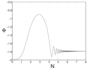
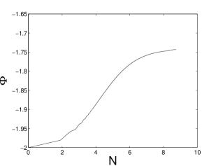
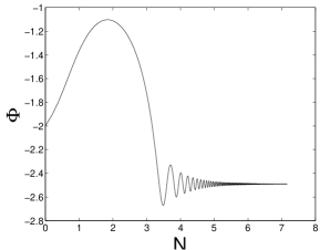
Figure 1: Numerical solutions which shows the gravitational potential $\Phi$ as a function of e-foldings after the end of inflation $N$ for three types of initial conditions. Leftmost panel: $\Phi=-2$, $\sigma_{*}=3$ and $\delta\sigma_{*}=0$. In this case the $\sigma$-field dominates before it starts oscillating. The final value of $\Phi$ agrees with eq. (27). Middle panel: $\Phi=-2$, $\sigma_{*}=0.3$ and $\delta\sigma_{*}=0$. In this case the $\sigma$-field does not dominate before it starts oscillating. The final value of $\Phi$ also agrees with eq. (27). Rightmost panel: $\Phi=-2$, $\sigma_{*}=3$ and $\delta\sigma_{*}=1$. This panel is identical to fig. 3 of [16].

3 The Axion

The main problem with the mechanism in the previous section compared to the naive example in eq.(2) is that the inhomogeneities in the radiation fluid gravitationally sources density perturbations in the $\sigma$-field fluid. In the case of the periodic form of an axion field potential it is well known that one can suppress the entropy perturbations in the axion fluid. One might think that one can circumvent the problems using this approach. However, as we will discuss below it will suffer from similar difficulties.

Neglecting again the decay rates, the change in the curvature perturbation $\zeta_{\sigma}$ in the $\sigma$-fluid is given by its intrinsic non-adiabatic pressure perturbation

$$\dot{\zeta}_{\sigma}=-\frac{H}{p_{\sigma}+\rho_{\sigma}}\delta P_{intr}~{},$$ (28)

where

$$\delta P_{intr}=\delta P_{\sigma}-c_{\sigma}^{2}\delta\rho_{\sigma}~{}.$$ (29)

In the ordinary curvaton limit, it is well known that $\delta\sigma$ behaves like $\sigma$ and $\delta P_{intr}$ vanishes [10]. It can be seen from eq.(2) that this holds even in the case where $\delta\sigma_{*}=0$ because of the gravitational sourcing. If we want $\dot{\zeta}_{\sigma}\neq 0$ in the relevant regimes, we need that the perturbations evolve differently than the background. This is true if the $\sigma$-field has a very non-linear periodic potential and we find it useful to examine this more thoroughly.

Let us assume that the field $\sigma$ is an axionic field for which the following potential is generated soon after the end of inflation

$$V(\sigma)=\frac{1}{2}V_{0}\left(1-\cos\left(\frac{\sigma}{\sigma_{0}}\right)\right)~{},$$ (30)

although one would have to worry, that a periodic potential will lead to formation of topological defects [21].

During the first ordinary slow-roll inflationary stage, the potential of the $\sigma$-field and its derivatives are insignificant, so the field fluctuation of the $\sigma$-field generated during inflation is simply

$$\delta\sigma^{2}=\frac{H_{i}^{2}}{4\pi^{2}}\ln\frac{aH_{i}}{k}~{}.$$ (31)

The linear approximation $\delta V(\sigma)\approx(dV(\sigma)/d\sigma)\delta\sigma$ is only valid if the $\sigma$-field and its dispersion is smaller than $\sigma_{0}$. As mentioned above we are interested in the non-linear limit. To understand the evolution of the density perturbations in this limit we can adopt the strategy originally proposed by Kofman and Linde [22, 23, 24]. At any given scale $l=1/k$ the field will consist of a large scale component that behaves as a homogeneous classical field $\sigma_{c}(k)$ and a shortwave part $\delta\sigma$ corresponding to momenta $k\geq 1/l$

$$\sigma=\sigma_{c}(k)+\delta\sigma~{}.$$ (32)

The effective classical field at the scale $1/l$ is the sum of the background vev $\tilde{\sigma}$ and its variance $\tilde{\sigma}_{k}$

$$\sigma_{c}(k)=\sqrt{\tilde{\sigma}^{2}+\tilde{\sigma}_{k}^{2}}~{}.$$ (33)

For $\tilde{\sigma}_{k}>>\sigma_{0}$ this implies

$$\sigma_{c}(k)^{2}\approx\tilde{\sigma}_{k}^{2}=\frac{H_{i}^{2}}{4\pi^{2}}\ln\frac{k}{k_{min}}~{}.$$ (34)

It was shown in [22, 23, 24], that the periodic nature of the axion field potential will then efficiently power-law suppress the axion density perturbations when $\sigma_{0}<<H$

$$\frac{\delta\rho_{\sigma}}{\rho_{\sigma}}\simeq\frac{\rho_{\sigma}}{\rho}\frac{H}{2\pi\sigma_{0}}\cos\left(\tilde{\sigma}_{c}(k)/\sigma_{0})\right)\left(\frac{k}{aH}\right)^{\frac{H^{2}}{8\pi^{2}\sigma_{0}^{2}}}~{}.$$ (35)

while for a non-flat spectrum for $\delta\sigma$ the suppression will be even exponential [2, 25]

$$\frac{\delta\rho_{\sigma}}{\rho_{\sigma}}\simeq\frac{\delta\sigma}{\sigma_{0}}\exp\left(-\frac{1}{2}\int_{k}^{k_{c}}d\ln k\frac{\delta\sigma^{2}}{\sigma_{0}^{2}}\right)$$ (36)

Above we used the approximations $\dot{\sigma}\approx 0$ and $\delta\rho_{\sigma}\approx\delta V(\sigma)$.

However, while this can lead to a significant suppression of entropy perturbations, in the separation of the field into the classical field and its fluctuations, we have to take into account that this separation will be different in each separate Hubble volume at the end of inflation. The adiabatic density perturbations can be understood to be a consequence of inflation not ending simultaneously everywhere due to the small inflaton fluctuations. At the end of inflation the observable universe today consisted of a huge number of causally separate Hubble patches whose relative evolution are synchronized by a relative time delay due to the inflaton fluctuations. No local physics can cancel this this synchronization, but one can produce additional adiabatic perturbations by converting entropy perturbation into adiabatic perturbations in each Hubble volume separately. Because of this time delay, the axion will also start to inflate and subsequently oscillate at slightly different times synchronized to the inflaton fluctuations in each different causally disconnected region. Thus, the separation of the field into the classical field and its fluctuations in eq.(32) will be shifted with respect to the synchronized time delay between each separate part of the universe, and if we take this into account the initial adiabatic fluctuation will remain imprinted in the axion fluid as it starts to dominate.

Acknowledgments

I would like to acknowledge Andreas Albrecht, Andrei Linde, Nemanja Kaloper, David Lyth, Slava Mukhanov, Misao Sasaki, Lorenzo Sorbo and David Wands for comments and criticism. Especially I would like to thank Andrei Linde, David Lyth, Slava Mukhanov, Misao Sasaki and David Wands for pointing out a problem in the first version. The work was supported in part by the DOE Grant DE-FG03-91ER40674.

References

- [1] A. H. Guth, Phys. Rev. D 23, 347 (1981); A. D. Linde, Phys. Lett. B 108, 389 (1982); B 114, 431 (1982); B 116, 335 (1982); B 116, 340 (1982); A. Albrecht and P. J. Steinhardt, Phys. Rev. Lett. 48, 1220 (1982).
- [2] K. Enqvist and M. S. Sloth, Nucl. Phys. B 626, 395 (2002) [arXiv:hep-ph/0109214].
- [3] D. H. Lyth and D. Wands, Phys. Lett. B 524, 5 (2002) [arXiv:hep-ph/0110002].
- [4] T. Moroi and T. Takahashi, Phys. Lett. B 522, 215 (2001) [Erratum-ibid. B 539, 303 (2002)] [arXiv:hep-ph/0110096].
- [5] S. Mollerach, Phys. Rev. D 42, 313 (1990).
- [6] A. D. Linde and V. Mukhanov, Phys. Rev. D 56, 535 (1997) [arXiv:astro-ph/9610219].
- [7] N. Bartolo, E. W. Kolb and A. Riotto, arXiv:astro-ph/0507573.
- [8] V. F. Mukhanov, H. A. Feldman and R. H. Brandenberger, Phys. Rept. 215, 203 (1992).
- [9] D. H. Lyth, C. Ungarelli and D. Wands, Phys. Rev. D 67, 023503 (2003) [arXiv:astro-ph/0208055].
- [10] M. S. Sloth, Nucl. Phys. B 656, 239 (2003) [arXiv:hep-ph/0208241].
- [11] K. A. Malik, D. Wands and C. Ungarelli, Phys. Rev. D 67, 063516 (2003) [arXiv:astro-ph/0211602].
- [12] C. Gordon and A. Lewis, Phys. Rev. D 67, 123513 (2003) [arXiv:astro-ph/0212248].
- [13] D. H. Lyth and D. Wands, Phys. Rev. D 68, 103516 (2003) [arXiv:astro-ph/0306500].
- [14] C. Gordon and K. A. Malik, Phys. Rev. D 69, 063508 (2004) [arXiv:astro-ph/0311102].
- [15] S. Gupta, K. A. Malik and D. Wands, Phys. Rev. D 69, 063513 (2004) [arXiv:astro-ph/0311562].
- [16] D. Langlois and F. Vernizzi, Phys. Rev. D 70, 063522 (2004) [arXiv:astro-ph/0403258].
- [17] F. Ferrer, S. Rasanen and J. Valiviita, JCAP 0410, 010 (2004) [arXiv:astro-ph/0407300].
- [18] G. Lazarides, R. R. de Austri and R. Trotta, Phys. Rev. D 70, 123527 (2004) [arXiv:hep-ph/0409335].
- [19] K. A. Malik and D. Wands, JCAP 0502, 007 (2005) [arXiv:astro-ph/0411703].
- [20] D. Wands, K. A. Malik, D. H. Lyth and A. R. Liddle, Phys. Rev. D 62, 043527 (2000) [arXiv:astro-ph/0003278].
- [21] A. D. Linde and D. H. Lyth, Phys. Lett. B 246, 353 (1990).
- [22] A. D. Linde, Phys. Lett. B 158, 375 (1985).
- [23] L. A. Kofman, Phys. Lett. B 173, 400 (1986).
- [24] L. A. Kofman and A. D. Linde, Nucl. Phys. B 282, 555 (1987).
- [25] R. Brustein and M. Hadad, Phys. Lett. B 442, 74 (1998) [arXiv:hep-ph/9806202].