Topics in quantum field theory: Renormalization groups in Hamiltonian framework and baryon structure in a non-local QCD model

”We are at the very beginning of time for the human race. It is not unreasonable that we grapple with problems. But there are tens of thousands of years in the future. Our responsibility is to do what we can, learn what we can, improve the solutions, and pass them on.”
                Richard Feynman

Declaration

No portion of the work referred to in this thesis has been submitted in support of an application for another degree or qualification of this or any other university, or other institution of learning.

Abstract

In this thesis I investigate aspects of two problems. In the first part of this thesis, I will investigate how an effective field theory can be constructed. One of the most fundamental questions in physics is how new degrees of freedom emerge from a fundamental theory. In the Hamiltonian framework this can be rephrased as finding the correct representation for the Hamiltonian matrix. The similarity (not essentially unitary) renormalization group provides us with an intuitive framework, where a transition from a perturbative region to a non-perturbative one can be realised and physical properties can be computed in a unified way. In this context, we have shown that the well-known coupled-cluster many-body theory techniques can be incorporated in the Wilsonian renormalization group to provide a very powerful framework for construction of effective Hamiltonian field theories. Eventhough the formulation is intrinsically non-perturbative, we have shown that a loop-expansion can be implemented.

The second part of my thesis is rather phenomenologically orientated. In this part, I will employ an effective field-theoretical model as can be constructed by means of the techniques of the first part of my thesis, a quark-confining non-local Nambu-Jona-Lasinio model and study the nucleon and diquarks in this model. For certain parameters the model exhibits quark confinement, in the form of a propagator without real poles. After truncation of the two-body channels to the scalar and axial-vector diquarks, a relativistic Faddeev equation for nucleon bound states is solved in the covariant diquark-quark picture. The dependence of the nucleon mass on diquark masses is studied in detail. We find parameters that lead to a simultaneous reasonable description of pions and nucleons. Both the diquarks contribute attractively to the nucleon mass. Axial-vector diquark correlations are seen to be important, especially in the confining phase of the model. We study the possible implications of quark confinement for the description of the diquarks and the nucleon. In particular, we find that it leads to a more compact nucleon.

General remarks

This thesis is organized as follows: in the first three chapters, we concentrate on renormalization group methods in Hamiltonian framework. In chapter 1, we introduce the coupled-cluster theory. In chapter 2, we show how renormalization group can be employed in the context of the coupled-cluster theory. In order to highlight the merits and the shortcomings of our approach over previous ones, in Sec. 2.2, we review different RG methods in Hamiltonian framework. Different aspects of our approach is introduced in sections 2.4-2.8. In sections 2.9 and 2.10, as illustrative examples, we apply our formulation on the $\Phi^{4}$ theory and an extended Lee model. In chapter 3, we pursue a different approach for the renormalization of the many-body problem. We show that a combination of the coupled-cluster theory and the Feshbach projection techniques leads to a renormalized generalized Brueckner theory.

In the second part of this thesis, we investigate the baryon structure in a chiral quantum chromodynamics model based on the relativistic Faddeev approach. In sections 4.1 and 4.2, we introduce the most important properties of QCD which are needed for the modelling of hadrons. In sections 4.3 and 4.4, we show how an effective low-energy field theory can be constructed from the underlying QCD theory. In chapter 5, we introduce alternative field theoretical approaches for describing baryons, such as Skyrme models, bag models and diquark-quark models in the context of the relativistic Faddeev approach. Finally, in chapter 6, we study baryons based on the diquark-quark picture in a quark-confining non-local NJL model. The non-local NJL model is introduced in Sec. 6.2. In Sec. 6.3, we discuss the pionic sector of the model. In Sec. 6.4 the diquark problem is solved and discussed. In Sec. 6.5 the three-body problem of baryons is investigated. The numerical technique involved in solving the effective Bethe-Salpeter equation is given and the results for three-body sector are presented.

Contents

1. 1 Basic structure of the coupled-cluster formalism
   1. 1.1 Introduction
   2. 1.2 Formalism
   3. 1.3 Linked-cluster theorem and Wightman functionals
2. 2 Hamiltonian renormalization Groups
   1. 2.1 Introduction
   2. 2.2 Traditional approaches and their problems
      1. 2.2.1 Glazek-Wilson formulation
      2. 2.2.2 Wegner Formulation
   3. 2.3 Coupling coherence condition
   4. 2.4 General formulation of the similarity renormalization group
   5. 2.5 The coupled-cluster renormalization group
   6. 2.6 The decoupling conditions versus the variational principle
   7. 2.7 The symplectic structure
   8. 2.8 The constrained induced phase space
   9. 2.9 Example I: $\Phi^{4}$ theory
   10. 2.10 Example II: Extended Lee Model
   11. 2.11 Conclusion
3. 3 Renormalization problem in many-body system
   1. 3.1 Introduction
   2. 3.2 The extended Lee Model
   3. 3.3 Nuclear matter equations
   4. 3.4 The renormalized nuclear matter equations
   5. 3.5 Conclusion
   6. 3.6 Some final remarks
4. 4 QCD properties and effective quark chiral models
   1. 4.1 QCD Symmetries
   2. 4.2 Non-perturbative features of QCD
   3. 4.3 Effective low-energy quark interaction
   4. 4.4 Fierz-transformation and the effective quark interaction
5. 5 QCD inspired pictures for baryons
   1. 5.1 Introduction
   2. 5.2 Baryons as chiral solitons; Skyrme model
   3. 5.3 Bag models
   4. 5.4 Diquark-quark picture; Relativistic Faddeev approach
6. 6 Baryons structure in a non-local quark confining NJL model
   1. 6.1 Introduction
   2. 6.2 A non-local NJL model
   3. 6.3 Meson channel
   4. 6.4 Diquark channels
      1. 6.4.1 Diquark Solution
   5. 6.5 Three-body sector
      1. 6.5.1 Numerical method for the coupled BS equations
      2. 6.5.2 Nucleon Solution
   6. 6.6 Summary and Outlook

Chapter 1 Basic structure of the coupled-cluster formalism

1.1 Introduction

In order to understand fully the properties of quantum many-body systems, various methods have been developed which aim to go beyond perturbation theory. One of the simplest approaches has been the so-called configuration-interaction method which diagonalises the Hamiltonian in a finite subspace of the full many-body Hilbert space. An extension of this method has been introduced via various versions of coupled-cluster methods [1, 2, 3, 4]. The coupled cluster method (CCM) in its simplest form originated in nuclear physics around forty years ago in the work of Coester and Kümmel [1]. The configuration-interaction method (CIM), and various version of coupled-cluster methods: normal coupled cluster method (NCCM)[1, 2] and the extended coupled cluster method (ECCM)[3, 4] form a hierarchy of many-body formulations for describing quantum systems of interacting particles or fields [5]. They are denoted generically as independent-cluster (IC) parametrizations, in the sense that they incorporate the many-body correlations via sets of amplitudes that describe the various correlated clusters within the interacting system as mutually independent entities. The intrinsic non-perturbative nature of the methods is considered to be one of their advantages which make them almost universally applicable in many-body physics. The IC methods differ from each other in the way they incorporate the locality and separability properties; in a diagrammatic language they differ in their linking properties. Each of the IC methods has been shown [4] to provide an exact mapping of the original quantum mechanical problem to a corresponding classical mechanics in terms of a set of multiconfigurational canonical field amplitudes. The merit of IC has been outlined in Ref. [5] and literature cited therein.

1.2 Formalism

In this section we concentrate on the NCCM and the ECCM from a formal viewpoint.

Exponential structures arise frequently in physics for similar underlying fundamental reasons. For example, in the Ursell-Mayer theory in statistical mechanics, in the Goldstone linked-cluster theorem [6] and the Gell-Mann and Low theorem [7]. The complexity of the vacuum (the ground state) of an arbitrary many-body system in the NCCM parametrization [1, 2, 5] is expressed by an infinite set of correlation amplitudes $\{s_{I},\tilde{s}_{I}\}$ which have to be determined by the dynamics,

$$|\psi\rangle=K(t)e^{S}|\psi_{0}\rangle,\hskip 56.9055pt\langle\tilde{\psi}|=\frac{1}{K(t)}\langle\psi_{0}|\tilde{S}e^{-S},$$

$$S=\sum_{I\neq 0}s_{I}C_{I}^{\dagger},\hskip 56.9055pt\tilde{S}=1+\sum_{I\neq 0}\tilde{s_{I}}C_{I}.\$$ (1.1)

Here $K(t)$ is a time-dependent scale factor. The coefficients $s_{I}$ and $\tilde{s_{I}}$ are time dependent. The intermediate normalization condition $\langle\tilde{\psi}|\psi\rangle=1$ is explicit for all times $t$. We restrict ourselves to the non-degenerate system, so that the exact states of the system may sensibly be refereed to some suitably chosen single reference state denoted as $|\psi_{0}\rangle$. The state $|\psi_{0}\rangle$ is a ground state, e.g. a special (Hartree) bare vacuum in quantum field theory (QFT). The function $|\psi_{0}\rangle$ can be chosen rather generally, but is tied to the choice of generalized creation operators $\{C^{{\dagger}}_{I}\}$; the state $|\psi_{0}\rangle$ is annihilated by $\{C_{I}\}$ $\forall I\neq 0$ (where $C_{0}\equiv 1$, the identity operator) and is a cyclic vector in the sense that the algebra of all possible operators in the many-body Hilbert space $\mathcal{H}$ is spanned by the two Abelian subalgebras of creation and annihilation operators defined with respect to it. In this way we can define proper complete orthonormal sets of mutually commuting configuration creations operators $\{C^{{\dagger}}_{I}\}$ and their Hermitian adjoint counterparts $\{C_{I}\}$, defined in terms of a complete set of many-body configuration $\{I\}$. These are, in turn, defined by a set-index $I$, which labels the cluster configuration created by $C^{{\dagger}}_{I}$ with respect to the reference state $|\psi_{0}\rangle$. Therefore, $\{I\}$ defines a subsystem or cluster within the full system of a given configuration and the actual choice of these clusters depends upon the particular system under consideration. We assume that the creation and annihilation subalgebras and the state $|\psi_{0}\rangle$ are cyclic, so that all ket states in the Hilbert space $\mathcal{H}$ can be constructed from linear combinations of states $\{C^{{\dagger}}_{I}|\psi_{0}\rangle\}$; and for the bra states with respect to states $\{\langle\psi_{0}|C_{I}\}$. It is well-known in the many-body application that the above parametrization Eq. (1.2), guarantees automatically proper size-extensivity (see section 1.3) and conformity with the Goldstone linked-cluster theorem [6] to all levels of truncation. In contrast, the configuration-interaction method is size extensive and linked only in the full, infinite-dimensional space [5]. The NCCM parametrization of bra- and ket-states Eq. (1.2), in its asymmetrical (independent) form, does not manifestly preserve their Hermitian congugacy, hence we have here a biorthogonal formulation of the many-body problem. However, this is the most reasonable parametrization if one is to preserve the canonical form of the equations of motion with respect to phase space $\{s_{I},\tilde{s}_{I}\}$ and the Hellmann-Feynman theorem [4, 5]. Nevertheless, non-hermiticity is negligible if the reference state and its complement are not strongly correlated [40]. We may hope that $S$ and $\tilde{S}$ are small (in a somewhat ill-defined non-perturbative sense), in other words, we may require that some of the coherence has already been obtained by optimizing the reference state. (This can be done, for example, by a Hartree-Bogolubov transformation). Then the remaining correlations can be added via the CCM. Therefore, defining a good reference state can in principle control the accuracy of CCM.

In the CIM, one defines the ket and bra states as follows,

$$|\psi\rangle=F|\psi_{0}\rangle;\hskip 56.9055pt\langle\tilde{\psi}|=\langle\psi_{0}|\tilde{F},$$

$$F=\sum_{I}f_{I}C^{{\dagger}}_{I};\hskip 56.9055pt\tilde{F}=\sum_{I}\tilde{f}_{I}C_{I},\$$ (1.2)

where the normalization condition $\langle\tilde{\psi}|\psi\rangle=1$ can not be imposed trivially. Although the CIM has a simpler parametrization than the CCM, it does not satisfy the size-extensivity after truncation and contains unlinked pieces emerging from the products of noninteracting subclusters. A formal relation between the CIM and coupled cluster theory will be demonstrated in section 1.3.

While all ground-state expectation values $\langle\tilde{\psi}|A|\psi\rangle=\bar{A}(s_{I},\tilde{s}_{I})$ and amplitudes $\{s_{I}\}$ are linked in NCCM, the amplitudes $\{\tilde{s_{I}}\}$ contain unlinked terms. This is resolved in the ECCM [3, 5] where we reparametrize the Hilbert space such that all basic amplitudes are linked,

$$|\psi\rangle=K(t)e^{S}|\psi_{0}\rangle;\hskip 56.9055pt\langle\tilde{\psi}|=\frac{1}{K(t)}\langle\psi_{0}|e^{\tilde{\Sigma}}e^{-S},$$

$$\Sigma|\psi_{0}\rangle=Qe^{\tilde{\Sigma}}e^{-S}S|\psi_{0}\rangle;\hskip 39.83368ptQ=1-|\psi_{0}\rangle\langle\psi_{0}|,$$

$$\Sigma=\sum_{I\neq 0}\sigma_{I}C^{{\dagger}}_{I};\hskip 78.24507pt\tilde{\Sigma}=\sum_{I\neq 0}\tilde{\sigma}_{I}C_{I}.\$$ (1.3)

The inverse relationships between the ECCM and the NCCM counterparts are given by

$$\sigma_{I}\equiv\langle\psi_{0}|C_{I}\tilde{S}S|\psi_{0}\rangle,\hskip 42.67912pts_{I}\equiv\langle\psi_{0}|C_{I}e^{\tilde{\Sigma}}\Sigma|\psi_{0}\rangle.$$ (1.4)

The ECCM amplitudes $\{\sigma_{I},\tilde{\sigma}_{I}\}$ are canonically conjugate (which comes from time dependent variation). It must be clear that this parametrization for the ECCM is not unique, however it is complete and sufficient to specify the ECCM phase space. It has been pointed out earlier that this choice of parametrization is the most convenient one [3]. The ECCM is believed to be the unique formulation of quantum many-body with full locality and separability at all levels of approximation. The individual amplitudes $\{s_{I},\tilde{s}_{I}\}$ (or $\{\sigma_{I},\tilde{\sigma}_{I}\}$) in both parametrizations are determined independently by solving an infinite set of non-linear equations which emerge from the dynamics of the quantum system. In practice, one needs to truncate both sets of coefficients. A consistent truncation scheme is the so called SUB($n$) scheme, where the $n$-body partition of the operator $\{s_{I},\tilde{s}_{I}\}$ (or $\{\sigma_{I},\tilde{\sigma}_{I}\}$) is truncated so that the general set-index $\{I\}$ contains up to $n$-tuple excitation (e.g., of single particle for bosonic systems with a reference state). Determination of the amplitudes corresponds to summing infinite sets of diagrams which in perturbation language take into account arbitrary high-order contributions in the coupling constant, therefore the NCCM and ECCM are not an expansion in this coupling constant. This property demands a precise truncation scheme for hierarchies without losing the renormalizability of the theory. We will consider this problem in the next chapter.

In the following, we confine our consideration to a real Klein-Gordon field, as an example. The configuration operators are specified by $\{C_{I}\to a_{k_{1}}...a_{k_{I}},C_{I}^{{\dagger}}\to a^{{\dagger}}_{k_{1}}...a^{{\dagger}}_{k_{I}}\}$ with subalgebra

$$[a_{k},a^{{\dagger}}_{k^{\prime}}]=\delta_{kk^{\prime}},\hskip 56.9055pt[a_{k},a_{k^{\prime}}]=0.$$ (1.8)

The corresponding $S$ and $\tilde{S}$ operators are

$$S=\sum_{n=1}S_{n},\hskip 56.9055ptS_{n}=\sum_{q_{1},..q_{n}}\frac{1}{n!}s_{n}(q_{1},..q_{n})a^{{\dagger}}_{q_{1}}..a^{{\dagger}}_{q_{n}},$$

$$\tilde{S}=1+\sum_{n=1}\tilde{S}_{n},\hskip 36.98866pt\tilde{S}_{n}=\sum_{q_{1},..q_{n}}\frac{1}{n!}\tilde{s}_{n}(q_{1},..q_{n})a_{q_{1}}..a_{q_{n}},\$$ (1.9)

and $|\psi_{0}\rangle$ is the Fock vacuum. The individual amplitudes $\{s_{n},\tilde{s}_{n}\}$ which describe excitations of $n$ Fock particles have to be fixed by the dynamics of the quantum system. Using Fock states in QFT has often been ambiguous due to problems connected with Haag’s theorem [9] (Haag’s theorem says that there can be no interaction picture - that we cannot use the Fock space of noninteracting particles as a Hilbert space - in the sense that we would identify Hilbert spaces via field polynomials acting on a vacuum at a certain time). It is well-known that the algebraic structure, does not, in general, fix the Hilbert space representation and therefore dynamical considerations are required. The IC formalism invokes dynamics rigorously. The dynamical principle to fix the physical vacuum is Poincaré invariance,

$$H|\psi\rangle=P|\psi\rangle=L|\psi\rangle=K|\psi\rangle=0,$$ (1.10)

where $H,P,L$ and $K$ are generators of the Poincaré group (Hamiltonian, momentum, angular momentum and boost operators, respectively). The excited states are no longer invariant under these symmetry operations and the spectrum can be obtained in an extended version of IC [10]. By putting the Ansatz Eqs. (1.2,1.2) into the conditions Eq. (1.10) one can obtain:

$$\langle q_{1},...,q_{n}|e^{-S}Pe^{S}|\psi_{0}\rangle=\langle q_{1},...,q_{n}|(P+[P,S])|\psi_{0}\rangle=\Big{[}\sum_{i=1}^{n}q_{i}\Big{]}s_{n}(q_{1},...,q_{n})=0,$$

(1.11)

$$\langle\psi_{0}|\tilde{S}e^{-S}Pe^{S}|q_{1},...,q_{n}\rangle=\langle\psi_{0}|\tilde{S}\big{(}P+[P,S]\big{)}|q_{1},...,q_{n}\rangle=\Big{[}\sum_{i=1}^{n}q_{i}\Big{]}\tilde{s}_{n}(q_{1},...,q_{n})$$

$$+\sum_{m}\frac{\tilde{s}_{n+m}(q_{1},...,q_{n+m})}{m!}\Big{[}[\sum_{i=1}^{m}q_{i}]s_{m}(q_{1},...,q_{m})\Big{]}=0,$$ (1.12)

$$\langle q_{1},...,q_{n}|e^{-S}Le^{S}|\psi_{0}\rangle=\sum_{\alpha}^{n}\epsilon_{ijl}(q_{\alpha})_{j}\frac{\partial}{\partial(q_{\alpha})_{l}}s_{n}(q_{1},...,q_{n})=0.\$$ (1.13)

In the same fashion one can impose the condition $\langle\psi_{0}|\tilde{S}e^{-S}Le^{S}|q_{1},...,q_{n}\rangle=0$, which leads to the following condition, having made used of the equation (1.13):

$$\sum_{\alpha=1}^{n}\epsilon_{ijl}(q_{\alpha})_{j}\frac{\partial}{\partial(q_{\alpha})_{l}}\tilde{s}_{n}(q_{1},...,q_{n})=0$$ (1.14)

Similarly for Hamiltonian and boost operators we have

$$\langle q_{1},...,q_{n}|e^{-S}He^{S}|\psi_{0}\rangle=\langle\psi_{0}|\tilde{S}e^{-S}He^{S}|q_{1},...,q_{n}\rangle=0,$$ (1.15)

$$\langle q_{1},...,q_{n}|e^{-S}Ke^{S}|\psi_{0}\rangle=\langle\psi_{0}|\tilde{S}e^{-S}Ke^{S}|q_{1},...,q_{n}\rangle=0.\$$ (1.16)

The equations (1.2,1.12,1.13,1.14) lead us to

$$s_{n}(q_{1},...,q_{n})=\delta\Big{[}\sum_{i=1}^{n}q_{i}\Big{]}s_{n}(\{q_{i}.q_{j}\}),\hskip 28.45274pt\tilde{s}_{n}(q_{1},...,q_{n})=\delta\Big{[}\sum_{i=1}^{n}q_{i}\Big{]}\tilde{s}_{n}(\{q_{i}.q_{j}\}),$$ (1.17)

which means that $\{s_{I},\tilde{s}_{I}\}$ depend on scalar quantities only and momentum is preserved. The same result can be obtained for the ECCM parametrization. To complete the determination of phase space, we use the energy hierarchy Eq. (1.15), where $H$ is a normal ordered Hamiltonian and the vacuum energy vanishes. Conceptually, it is evident that Eq. (1.15) suffices to fix all amplitudes without invoking Eq. (1.16), but explicit verification to all orders seems to be impossible.

The fully linked feature of the $e^{-S}He^{S}$ term in Eq. (1.15) can be made explicit by denoting it as $\{He^{S}\}_{\mathcal{L}}$, which can be written as a set of nested commutators,

$$e^{-S}He^{S}=\{He^{S}\}_{\mathcal{L}}=H+[H,S]+\frac{1}{2!}[[H,S],S]+...\hskip 28.45274pt.$$ (1.18)

This procedure is still rigorous. Lorentz symmetry, stability and causality are examples of features normally expected to hold in physical quantum field theories. In renormalized QFT stability and causality are closely intertwined with Lorentz invariance. For example, stability includes the need for energy positivity of Fock states of ordinary momenta, while causality is implemented microscopically by the requirement that observables commute at spacelike separation [11], so-called microcausality. In addition, both are expected to hold in all inertial frames. A stable and causal theory without Lorentz symmetry could in principle still be acceptable [12]. In the framework of many-body theory, medium contributions always affect the local and global properties of hadrons especially at high density. In dense matter, the Pauli principle and cluster properties can affect causality since they restrict the permissible process in a scattering reaction. To understand these effects we need firstly to consider if our formalism itself can in principle preserve the causal structure of given physical system. Let us introduce a new set $\{b_{k},b_{k}^{{\dagger}}\}$ which are connected to previous $\{a_{k},a_{k^{\prime}}^{{\dagger}}\}$ defined in Eq. (1.8) via a generalized Bogolubov transformation,

$$b^{{\dagger}}_{k}=A_{ki}a^{{\dagger}}_{i}+B_{ki}a_{i}+D_{i},$$ (1.19)

This is the most general linear transformation, which preserves commutator relations ($b_{k}$ is an annihilation operator and $b^{{\dagger}}_{k}$ is the Hermitian conjugate of $b_{k}$),

$$[b_{k},b^{{\dagger}}_{k^{\prime}}]=\delta_{kk^{\prime}},\hskip 56.9055pt[b_{k},b_{k^{\prime}}]=0,$$ (1.20)

provided that $AA^{{\dagger}}-BB^{{\dagger}}=1$. This obviously preserves the commutator relations for boson fields and preserves microcausality explicitly. The bare “$a$ vacuum” defined by $a_{k}|\psi_{0}\rangle_{a}=0$, is replaced by a bare “$b$ vacuum” which satisfies $b_{k}|\psi_{0}\rangle_{b}=0$. Using Thouless theorem [14], $|\psi\rangle_{b}$ can be written as

$$|\psi\rangle_{b}=N^{-1/2}e^{S_{1}+S_{2}}|\psi\rangle_{a},$$ (1.21)

with

$$S_{1}=\sum_{k}S^{1}_{k}(A,B,D)a^{{\dagger}}_{k},\hskip 42.67912ptS_{2}=\sum_{kk^{\prime}}\frac{1}{2!}S^{2}_{kk^{\prime}}(A,B,D)a^{{\dagger}}_{k}a^{{\dagger}}_{k^{\prime}},$$ (1.22)

where $S^{1}$ and $S^{2}$ are known functions of the matrices $A$ and $B$ and the vector $D$ [14]. It is obvious that $|\psi\rangle_{b}$ is a low-order approximation to the CCM wave function Eq. (1.2) or (1.2). The above-mentioned parametrization of vacuum wave function can be generalized to the CCM wave function, however it may require a nonlinear transformation from which it can be constructed. The inspiration for this transformation can be taken from the extension IC formulation for excited states [10]

$$b^{{\dagger}}_{k}=e^{S}F(k),\hskip 56.9055ptF(k)=a_{k}^{{\dagger}}+\sum_{n=3}^{\infty}F_{n}(p_{1},...,p_{n-1},k)a^{{\dagger}}_{p_{1}}...a^{{\dagger}}_{p_{n-1}},$$ (1.23)

where the correlation operator $S$ is known from Eq. (1.2) and $F$ is a new amplitude which includes momentum conservation. This new amplitudes has to be determined and it changes the momentum of the bosons before creation. It is not hard to derive equations for the energy spectrum which lead us to $N$-body effective Hamiltonians [15] and yields the folded diagrams of degenerate many-body perturbation theory [16]. This nonlinear transformation manifestly invalidates the commutator relation Eq. (1.20) and accordingly the microcausal commutation relations of the boson field. It should be noted that causality of the underlying theory can not be fully determined at this level and one needs to take into account the dynamics of the underlying quantum system. Causality in the context of IC formulation can be ensured by requiring

$$\langle\tilde{\psi}|[\phi(X),\phi(Y)]|\psi\rangle=0,\hskip 56.9055pt(X-Y)^{2}<0,$$ (1.24)

where $Y$ denotes space-time coordinates $(y,y_{0})$ and $\phi(Y)$ is Klein-Gordon field operator which is expressed in terms of Fock space operators by

$$\phi(Y)=\sum_{k}\xi(Y)_{k}a_{k}+\xi^{{\dagger}}_{k}(Y)a^{{\dagger}}_{k},$$ (1.25)

where $\xi_{k}(Y)$ form a complete orthonormal set of states. Eq. (1.24) can be evaluated explicitly by using the following identity [4, 5]

$$\langle\tilde{\psi}|[A,B]|\psi\rangle=\overline{[A,B]}=\sum_{I}\frac{\partial\bar{A}}{\partial{x_{I}}}\frac{\partial\bar{B}}{\partial{\tilde{x}_{I}}}-\frac{\partial\bar{A}}{\partial{\tilde{x}_{I}}}\frac{\partial\bar{B}}{\partial{x_{I}}},$$ (1.26)

where $\{x_{I},\tilde{x}_{I}\}$ are the canonical coordinate and momenta of the NCCM or the ECCM parametrization. By making use of Eqs. (1.2,1.18) and (1.25) one can find

$$\langle\tilde{\psi}|\phi(Y)|\psi\rangle=\overline{\phi(Y)}=\sum_{n=1}\sum_{k}\xi_{k}(Y)\tilde{x}_{n-1}(q_{1},...,q_{n-1})x_{n}(q_{1},...,q_{n-1},k)+\xi^{{\dagger}}_{k}(Y)\tilde{x}_{1}(k),$$ (1.27)

where $\{x_{n}\to s_{n},\sigma_{n},\tilde{x}_{n}\to\tilde{s}_{n},\tilde{\sigma}_{n}\}$ and we define $\tilde{x}_{0}=1$. By exploiting Eq. (1.26) one can show

$$\overline{[\phi(X),\phi(Y)]}=\sum_{k,k^{\prime}}[\xi_{k}(X)\xi^{{\dagger}}_{k^{\prime}}(Y)-\xi^{{\dagger}}_{k}(X)\xi_{k^{\prime}}(Y)]=\Delta(X-Y)-\Delta(Y-X).$$ (1.28)

The function $\Delta(X-Y)$ is the Pauli-Jordan function [11] defined for field operators expanded in plane-wave basis. When $(X-Y)^{2}<0$, we can perform a Lorentz transformation on the second term, taking $(X-Y)\to-(X-Y)$. The two terms are therefore equal and cancel to give zero, hence, Eq. (1.24) is satisfied. It should be noted that for a general quantum system by considering just the dynamics of the underlying system, determining the amplitudes $\{x_{I},\tilde{x}_{I}\}$ and verifying Eq. (1.24) at every level of truncation one can ensure causality. Obviously this might introduce a lower limit of truncation in a consistent SUB(n) scheme which contains causality.

In relativistic quantum mechanics there is another distinct type of causality, the fact that there is a well-posed initial value problem, so-called Cauchy causality. In the local field theory the Poincaré invariance implies the existence of a unitary representation of the Poincaré group that acts on the Hilbert space. In other words, the transformed final state is uniquely determined by time evolving the transformed initial state. Therefore, Cauchy causality is a consequence of Poincaré invariance and is independent of any consideration concerning microcausality.

One of the standard approaches in the nuclear many-body theory is to introduce an effective interaction and reduce the full many-body problem to a problem in a small model-space. As an example for the meson-nucleon system below threshold, it was shown that one has either hermitian effective operators with all desirable transformation properties under the Poincaré group or non-hermitian ones obtained by the CCM with desirable simplicity [13]. Thus effective operators introduced by the CCM can not manifestly preserve Cauchy causality, at any level of truncation. However, it economically disentangles and reduces the complexities of the many-body problem. It is notable that in some cases, the violation of relativistic invariance due to truncation is consistent with errors introduced via the approximation [14]. In practice one should not expect that Poincaré invariance holds for an approximation, and forcing the approximated wave function to obey Lorentz invariance might lead to inconsistent results. Having said that, we will show that in the context of coupled-cluster renormalization group framework, one can in principle define a truncation scheme where Poincaré invariance is preserved.

1.3 Linked-cluster theorem and Wightman functionals

In this section we proceed from a formal view to show the relation between the CIM and the coupled cluster method. We will show that the CCM is a natural reparametrization of the CIM which incorporates the full size-extensivity. For this purpose we exploit the reconstruction theorem [17], well known in axiomatic Quantum field theory [18]:

Denote the state vector of the vacuum by $|\Omega\rangle$ (in the language of the CCM $|\Omega\rangle$ is the full interacting ground state $|\psi\rangle$). The physical vacuum expectation value of products of local fields

$$w^{n}(x_{1}...x_{n})=\langle\Omega|\phi(x_{1})...\phi(x_{n})|\Omega\rangle,$$ (1.29)

are tempered distributions over $\mathbb{R}^{4n}$. These $w^{n}$ are called Wightman distributions. If the hierarchy of distributions $w^{n}(n=0,...)$ is known then the Hilbert space can be constructed. This is the so-called reconstruction theorem [17].

Now consider a configuration $(x_{1},...,x_{n})$ consisting of several clusters. A cluster here is a subset of points so as all the points in one cluster have a large space-like separation from all the points in any other clusters. One may expect that in infinite separation between the clusters, one has

$$w^{n}(x_{1},...,x_{n})\sim\prod_{r}w^{n_{r}}(y_{r,1},...y_{r,n_{r}}),$$ (1.30)

the index $r$ and $n_{r}$ denote the cluster and number of points in the $r$-th cluster, respectively. $y_{r,n_{k}}$ indicates a subset of the $x_{k}$ belonging to this cluster. Thus we require that in the vacuum state the correlation of quantities relating to different regions decreases to zero as the space-like separation of the regions increases to infinity. Therefore it makes sense to introduce another hierarchy of functions $w^{n}_{T}$,

$$w^{n}(x_{1},...,x_{n})=\sum_{p}\prod_{r}w^{n_{r}}_{T}(y_{r,k}).$$ (1.31)

Here $p$ denotes a partition of the set of points $x_{i}$ into subsets labeled by the index $r$. The sum is over all possible partitions, The objects $w^{n}_{T}$ are called truncated functions or correlated functions. Within the hierarchy $\{w^{n}\}$ the truncated functions can be computed recursively:

$$w^{1}_{T}(x)=w^{1}(x),$$

$$w^{2}_{T}(x_{1},x_{2})=w^{2}(x_{1},x_{2})-w^{1}(x_{1})w^{1}(x_{2}),$$ (1.32)

$$\vdots\$$

The asymptotic property Eq. (1.30) of the $w^{n}$ is converted to the simpler property

$$w^{n}_{T}(x_{1},...x_{n})\to 0,$$ (1.33)

if any space like separation $x_{i}-x_{j}$ goes to infinity.

Let us now consider a hierarchy of functions $P^{n}(k_{1},...k_{n})$ (for simplicity totally symmetric under permutation of their arguments). We define a generating functional $\mathcal{P}\{f\}$ for an arbitrary function $f(k)$:

$$\mathcal{P}\{f\}=\sum_{n}\frac{1}{n!}\int P^{n}(k_{1},...k_{n})f(k_{1})...f(k_{n}).$$ (1.34)

The $P^{n}$ can be found from

$$P^{n}(k_{1},...k_{n})=\frac{\delta^{n}}{\delta f(x_{1})..\delta f(x_{n})}\mathcal{P}\{f\}|_{f=0}.$$ (1.35)

Now one can simply use the definition Eq. (1.31) to obtain a relation between the hierarchy $\{P^{n}\}$ and the hierarchy of the truncated functions $\{P^{n}_{T}\}$ in terms of respective generating function, namely

$$\mathcal{P}\{f\}=e^{\mathcal{P}_{T}\{f\}}.$$ (1.36)

This relation is called the Linked cluster theorem [18]. Having in mind the relations Eqs. (1.34) and (1.36), one observes that the CCM parametrization introduced in Eqs. (1.2) and (1.2) is a natural reparametrization of the CIM defined in Eq. (1.2) which incorporates the size-extensivity [5], at finite levels of truncation. This leads to a cluster decomposition and linked decomposition property of CCM at any level of truncation. Thus for extensive variables as the energy, the linked terms lead to contributions which obey the proper linear scaling in the particle number. The CIM contains unlinked diagrams for the ground-state energy expectation value, and thereby suffers from the so-called size-extensivity problems.

The cluster decomposition condition Eq. (1.30) is fundamental to a quantum field theory. It may break down partly when, in a statistical-mechanical sense, the theory is in a mixed phase [19]. This implies that there is more than one possible vacuum state, and therefore the cluster decomposition should be restored in principle if one builds the Hilbert space on one of the vacua.

Notice that in QCD, the cluster decomposition for colour singlet objects can break down due to the confinement. In axiomatic local quantum field theory with an indefinite metric space $\nu$ (e.g., Minkowski space) the following theorem holds; for the vacuum expectation values of two (smeared local) operators $A$ and $B$ with spacelike distance $R$ from each other [20, 21]:

$$|\langle\Omega|A(x)B(0)|\Omega\rangle - \langle\Omega|A(x)|\Omega\rangle\langle\Omega|B(0)|\Omega\rangle|$$ (1.39)

$$\leq \left\{\begin{array}[]{ll}\text{const}\times R^{-3/2+2N}e^{-MR}&\text{if there is a mass gap M},\\ \text{const}\times R^{-2+2N}&\text{if there is no mass gap},\end{array}\right.\$$

where $M$ is the mass gap. (Herein, we assume $N=0$, however, a positive $N$ is possible for the indefinite inner product structure in $\nu$.) In order to avoid the decomposition property for product of unobservable operators $A$ and $B$ which together with Kugo-Ojima criterion [20, 22] for the confinement is equivalent to failure of the decomposition property for coloured clusters, there can not be a mass gap in the indefinite space $\nu$. This would thus eliminate the possibility of scattering a physical state into color singlet states consisting of widely separated colored clusters (the “behind-the-moon” problem). However, this has no information for the physical spectrum of the mass operator in $\mathcal{H}$ which indeed does have a mass gap. In another words, there is a mass gap (but not in the full indefinite space $\nu$) in the semi-definite physical subspace induced by the BRST charge operator $Q_{B}$, $\nu_{\text{phy}}=\text{Ker}Q_{B}$, where states within are annihilated by $Q_{B}$,

$$v_{\text{phys}} = \{|\psi\rangle\in v:Q_{B}|\psi\rangle=0\}=\text{Ker}Q_{B},$$

$$\mathcal{H}(Q_{B},v) = \text{Ker}Q_{B}/\text{Im}Q_{B},\$$ (1.40)

where states in $\text{Im}Q_{B}=(\text{Ker}Q_{B})^{\bot}$ are called BRST-coboundaries in the terminology of de Rham cohomology and do not contribute in $\nu_{\text{phys}}$ [23]. It has been shown [24] that there is a connection between Kugo-Ojima criterion and an infrared enhancement of the ghost propagator. In Landau gauge, the gluon-ghost vertex function offers a convenient possibility to define a non-perturbative running coupling. The infrared fixed point obtained from this running coupling determines the two-point color-octet interactions and leads to the existence of unphysical massless states which are necessary to escape the cluster decomposition of colored clusters [20]. Notice that a dynamical mechanism, responsible for breaking of cluster decomposition for colored objects, is yet to be discovered, since our knowledge about color confinement is still preliminary.

Chapter 2 Hamiltonian renormalization Groups

2.1 Introduction

The main goal of traditional renormalization theory is to determine when and how the cancellation of divergences originating from the locality of quantum field theory may occur. This is essential if one wants to have meaningful quantitative results. However, it is by no means obvious how quantum fluctuations associated with short distance scales can be incorporated and controlled through the choice of only a few parameters, typically the bare masses and coupling constants, or by the counterterms in renormalized perturbation theory.

The development of Wilson’s renormalization group (RG) formalism [25] allowed physicists to produce a logically consistent picture of renormalization in which perturbation theory at arbitrary high energy scale can be matched with the perturbation expansion at another scale, without invoking the details of intermediate scales. In the Wilsonian approach, all of the parameters of a renormalizable field theory can be thought of as scale-dependent objects and their flows are governed by the so-called RG differential equations.

Motivated by Wilson’s picture, effective field theory (EFT) approaches have been introduced to replace complicated fundamental theories with simpler theories based only on the relevant degrees of freedom at the physical scale of interest [26]. The basis of the EFT concept is the recognition of the importance of different typical energy scales in nature, where each scale has its own characteristic degrees of freedom. In strong interactions the transition from the fundamental to the effective level is induced by a phase transition that takes place around $\Lambda_{\text{QCD}}\simeq 1\text{GeV}$ via the spontaneous breaking of chiral symmetry, which generates pseudoscalar Goldstone bosons. This coincides, of course, with the emergence of nuclei and nuclear mather, as opposed to the quark-gluon plasma and quark matter expected to occur at high temperature and high density. Therefore, at low energies ($E<\Lambda_{\text{QCD}}$), the relevant degrees of freedom are not quarks and gluons, but pseudoscalar mesons and other hadrons. The resulting description is a chiral EFT, which has much in common with traditional potential models. In particular, there might be an intermediate regime where a non-relativistic model is inadequate but where relatively few hadronic degrees of freedom can be used to faithfully describe both nuclear structure and response. If this is the case, one should be able to describe strongly interacting hadronic systems in this effective model.

The power of Hamiltonian methods is well known from the study of non-relativistic many-body systems and from strongly-interacting few particle systems, even though a Lagrangian approach is usually chosen for relativistic theories. One might prefer to obtain the effective interaction using the covariant Lagrangian formalism and then consider the ground state and collectively excited states in the non-covariant Hamiltonian formalism by exploiting many-body techniques. For the description of physical states and in particular bound states, the Hamiltonian formalism is preferable over the Lagrangian one. This is due to the fact that such problems are not naturally defined covariantly. For a bound state the interaction time scale is infinite, and thus a time-independent approach is better suited. However, the Lagrangian can not generally be converted to a Hamiltonian if the effective Lagrangian contains higher-order time-derivatives, since no Legendre transformation exits for such a case. Therefore one may wish to obtain the effective interaction in a unified self-consistent way within the Hamiltonian formalism. The renormalization group transformation is used to derive the physical Hamiltonian that can describe experiment. To implement a RG calculation, one should define a space of Hamiltonians and find a certain RG transformation which maps this space into itself. Then one should study the topology of the Hamiltonian space, by searching for the fixed points and studying the trajectories of the Hamiltonian with respect to these fixed points. At the fixed points we have a scale-invariant quantum field theory. Near the fixed point, the irrelevant operators in the original Hamiltonian have small coefficients, and we are only left with the relevant and marginal operators. The coefficients of these operators correspond to the parameters of the renormalized field theory. In this way, in a renormalizable field theory, we disregard information about the evolution of irrelevant terms. The fact that irrelevant terms can be dropped near the fixed point does not necessarily imply that they are unimportant at low-energy scales of experimental interest. This depends on how sensitive the physical observables are to physics near the scale of the cutoff. Therefore, it is of interest to develop a RG method in which the irrelevant variables are treated on an equal footing with the relevant and marginal variables (the schemes presented here have this advantage).

Hamiltonian methods for strongly-interacting systems are intrinsically non-perturbative and usually contain a Tamm-Dancoff type approximation, in the sense that one expands the bound state in states containing a small number of particles. This truncation of the Fock space gives rise to a new class of non-perturbative divergences, since the truncation does not allow us to take into account all diagrams for any given order in perturbation theory. Therefore renormalization issues have to be considered carefully. Two very different remedies for this issue are the use of light-front Tamm-Dancoff field theory (LFFT) [27] and the application of the coupled cluster method (CCM) [5, 28]. However, both methods are too complicated to attack the issue in a self-consistent way. In the last decade extensive attempts have been made to give a workable prescription for renormalization within the Hamiltonian formalism [29, 30, 31, 32]. Commonly unitary transformations are used to decouple the high- and low-energy modes aiming at the partial diagonalization of the Hamiltonian. One of the most elegant approaches in this context is the similarity renormalization group (SRG) proposed by Glazek and Wilson [29] (and by Wegner [30] independently). The SRG [29, 30] is designed to be free of small energy denominators and to eliminate interactions which change the energies of the unperturbed states by a large amount. However, there are several problems with this approach: it is hard to incorporate loop expansions within the method, the SRG can not systematically remove interactions which change the number of particles (i.e, when the Hamiltonian is not diagonal in particle number space), and most importantly, the computations are complex and there is no efficient non-perturbative calculation scheme.

In this chapter we introduce a new method [32, 33] for obtaining the low-energy effective operators in the framework of a CCM approach. The transformation constructed avoids the small denominators that plague old-fashioned perturbation theory. Neither perturbation theory nor unitarity of the transformation are essential for this method. The method is non-perturbative, since there is no expansion in the coupling constant; nonetheless, the CCM can be conceived as a topological expansion in the number of correlated excitations. We show that introducing a double similarity transformation using linked-cluster amplitudes will simplify the partial diagonalization underlying renormalization in Hamiltonian approaches. However, a price must be paid: due to the truncation the similarity transformations are not unitary, and accordingly the hermiticity of the resultant effective Hamiltonian is not manifest. This is related to the fact that we have a biorthogonal representation of the given many-body problem. There is a long tradition of such approaches. The first we are aware of are Dyson-type bosonization schemes [34]. [Here one chooses to map the generators of a Lie algebra, such that the raising generators have a particularly simple representation.] The space of states is mapped onto a larger space where the physically realizable states are obtained by constrained dynamics. This is closely related to CCM formalism, where the extended phase space is a complex manifold, the physical subspace constraint function is of second class and the physical shell itself is a Kähler manifold [35]. The second is the Suzuki-Lee method in the nuclear many-body (NMT) problem [36, 37], which reduces the full many-body problem to a problem in a small configuration space and introduces a related effective interaction. The effective interaction is naturally understood as the result of certain transformations which decouple a model space from its complement. As is well known in the theory of effective interactions, unitarity of the transformation used for decoupling or diagonalization is not necessary. Actually, the advantage of a non-unitarity approach is that it can give a very simple description for both diagonalization and ground state. This has been discussed by many authors [38] and, although it might lead to a non-hermitian effective Hamiltonian, it has been shown that hermiticity can be recovered [35, 39]. Notice that defining a good model space can in principle control the accuracy of CCM [40, 41].

To solve the relativistic bound state problem one needs to systematically and simultaneously decouple 1) the high-energy from low-energy modes and 2) the many- from the few-particle states. We emphasize in this chapter that CCM can in principle be an adequate method to attack both these requirements. Our hope is to fully utilize Wilsonian Exact renormalization group [25] within the CCM formalism. Here the high energy modes will be integrated out leading to a modified low-energy Hamiltonian in an effective many-body space. Notice that our formulation does not depend on the form of dynamics and can be used for any quantization scheme, e.g., equal time or light-cone.

2.2 Traditional approaches and their problems

The Tamm-Dancoff approximation [42] was developed in the 1950’s to describe a relativistic bound state in terms of a small number of particles. It was soon revealed that the Tamm-Dancoff truncation gives rise to a new class of non-perturbative divergences, since the truncation does not allow us to take into account all diagrams at a given order in perturbation theory. On the other hand, any naive renormalization violates Poincaré symmetry and the cluster decomposition property (the cluster decomposition means that if two subsystems at very large space-like separation cease to interact then the wave function becomes multiplicatively separable). One of the simplest example of the Tamm-Dancoff approximation is the constituent picture of QCD where one describes a QCD bound state $|\psi\rangle$ within a truncated Fock-space,

$$|\psi\rangle=\phi_{1}|q\bar{q}\rangle+\phi_{2}|q\bar{q}g\rangle+\phi_{3}|q\bar{q}q\bar{q}\rangle+...$$

we use a shorthand notation for the Fock-space where $q$ is a quark, $\bar{q}$ an antiquark, and $g$ stands for a gluon. Now the bound-state problem is solved via the Schrödinger equation $H^{QCD}|\psi\rangle=E|\psi\rangle$. It is well known that in the complicated equal-time vacuum bound states contain an infinite number of particles that are part of the physical vacuum on which hadrons are built. On the other hand, interactions in a field theory couple states with arbitrarily large difference in both free energy and numbers of particles. Thus any Fock-space expansion can hardly be justified without being supplemented with a prescription for decoupling of the high-energy from the low-energy modes and the many-body from few-particle states. In the context of the Hamiltonian formulation this problem can be expresed by asking how the Hamiltonian matrix is diagonalized in particle- and momentum-space.

In his earliest work Wilson[43] exploited a Bloch type transformation [44] to reduce the Hamiltonian matrix by lowering a cutoff which was initially imposed on the individual states. Later Wilson abandoned this formulation in favour of a Lagrangian one. The most important reason was that the Bloch transformation is ill-defined and produces unphysical divergences. These divergences emerge from denominators which contain a small energy difference between states retained and states removed by the transformation, and appear across the boundary line at $\lambda$ .

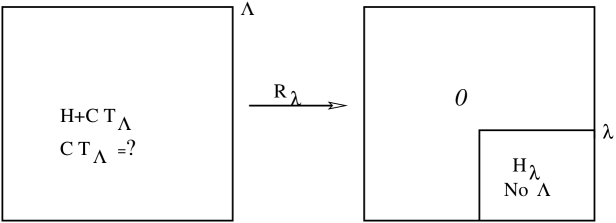
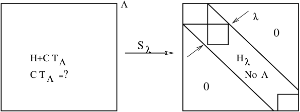
Figure 2.1: Two ways to run a cutoff on free energy. In top a cutoff on the magnitude of the energy is lowered from $\Lambda$ to $\lambda$, leading to a small matrix (this scheme corresponds to the original Wilson RG). In down we show similarity renormalization group scheme where a cutoff is imposed on the off-diagonal part of the matrix and diagonalization is led to a narrow matrix with a band width $\lambda$. $CT_{\Lambda}$ denotes the counterterms.

Two remedies for this issue are the use of light front coordinates [27] and application of the CCM [28]. In the light-front Tamm-Dancoff field theory (LFFT) the quantization plane is chosen to coincide with the light front, therefore the divergences that plagued the original theories seem to disappear [45] since here vacuum remains trivial. Furthermore, not having to include interactions in boost operators allows a renormalizable truncation scheme [46]. One of the most important difficulties in LFFT is the complicated structure of the renormalization process [47]. In principle, ad-hoc counterterms can not be prevented if one is to preserve the underlying symmetry. In the standard form of CCM, on the other hand, the amplitudes obey a system of coupled non-linear equations which contain some ill-defined terms because of ultraviolet divergences. It has been shown [48] that the ill-defined amplitudes, which are also called critical topologies, can be systematically removed, by exploiting the linked-cluster property of the ground state. This can be done by introducing a mapping which transfers them into a finite representations without making any approximation such as a coupling expansion. Thus far this resummation method has been restricted to superrenormalizable theories due to its complexity.

Recently Wilson and Glazek [29] and independently Wegner [30] have re-investigated this issue and introduced a new scheme, the similarity renormalization group (SRG). The SRG resembles the original Wilsonian renormalization group formulation [43], since a transformation that explicitly runs the cutoff is developed. However, here one runs a cutoff on energy differences rather than on individual states. In the SRG framework one has to calculate a narrow matrix instead of a small matrix, and the cutoff can be conceived as a band width (see Fig. [2.1]). Therefore by construction the perturbation expansion for transformed Hamiltonians contains no small-energy denominators. Here we review the general formulation of the SRG.

2.2.1 Glazek-Wilson formulation

The detailed description of Glazek-Wilson RG method can be found in Ref. [29]. Here we only concentrate on the key elements of their method. We introduce a unitary transformation aiming at partially diagonalizing the Hamiltonian so that no couplings between states with energy differences larger than $\lambda$ are present. The unitary transformation defines a set of Hamiltonians $H_{\lambda}$ which interpolate between the initial Hamiltonian ($\lambda=\Delta$ ) and the effective Hamiltonian $H_{\lambda}$. This $\lambda$ plays the role of a flow parameter. We will assume that $H_{\lambda}$ is dominated by its diagonal part which we will denote $H_{0\lambda}$ with eigenvalues $E_{i\lambda}$ and eigenstates $|i\rangle$:

$$\langle f|H_{0\lambda}|i\rangle=E_{i\lambda}\langle f|i\rangle.$$ (2.1)

Therefore the Hamiltonian at scale $\lambda$ can be written $H_{\lambda}=H_{0\lambda}+H_{I\lambda}$, where $H_{I\lambda}$ is non-diagonal part. Notice that $H_{0\lambda}$ is not necessarily the bare free Hamiltonian which is independent of $\lambda$. In order to introduce the infinitesimal unitary transformations which induce the infinitesimal changes in $H_{\lambda}$ when $\lambda$ changes by an infinitesimal amount, we need to define various zones of the operators We introduce an auxiliary function $x_{ij\lambda}=\langle i|x_{\lambda}|j\rangle$ of the states with labels $i$ and $j$ for a given $\lambda$. If we denote the eigenvalue of $H_{0\lambda}$ with $E_{i\lambda}$, $x$ is defined as

$$x_{ij\lambda}=\frac{|E_{i\lambda}-E_{j\lambda}|}{E_{i\lambda}+E_{j\lambda}+\lambda}.$$ (2.2)

The modulus of the function $x_{ij\lambda}$ is close to $1$ when one of the energies is much larger than the other and also much larger than the cutoff $\lambda$ and $x$ approaches $0$ when the energies are similar or small in comparison to the cutoff. One then introduces smooth projectors

$$u_{ij\lambda}=\langle i|u_{\lambda}|j\rangle=u(x_{ij\lambda}),$$ (2.3)

and

$$r_{ij\lambda}=1-u_{ij\lambda}=r(x_{ij\lambda}).$$ (2.4)

By means of $u$ and $r$ one can separate each matrix into two parts $M=D(M)+R(M)$, where we define

$$D(M)_{ij}=u_{ij\lambda}M_{ij},$$ (2.5)

and corresponding

$$R(M)_{ij}=r_{ij\lambda}M_{ij}.$$ (2.6)

The functions $u$ and $r$ are needed in order to ensure smoothness and differentiability, and consequently a continuous transition between different parts of the Hamiltonian matrix. They are the key elements in making the diagonalization free of small-energy denominators. These functions are implemented as a “form factor“ in every vertex of the interaction. We construct an infinitesimal unitary transformation eliminating the part of Hamiltonian which has only non-zero elements far away from the diagonal, thus they can not produce small-energy denominators. This continuous unitary transformation satisfies,

$$\frac{dH_{\lambda}}{d\lambda}=[T_{\lambda},H_{\lambda}].$$ (2.7)

The generator $T_{\lambda}$ is anti-Hermitian and is chosen in such a way that

$$H_{\lambda}=D(Q_{\lambda})=Q_{\lambda}u_{\lambda},$$ (2.8)

where $Q$ is arbitrary in the far-off-diagonal region. In terms of $Q$, the matrix elements of Eq. (2.7) satisfy

$$\frac{du_{ij\lambda}}{d\lambda}Q_{ij\lambda}+u_{ij\lambda}\frac{dQ_{ij\lambda}}{d\lambda}=T_{ij\lambda}(E_{j\lambda}-E_{i\lambda})+[T_{\lambda},H_{I\lambda}]_{ij}.$$ (2.9)

Notice that $Q_{\lambda}$ can be arbitrary in the far-off diagonal region where $u_{\lambda}=\frac{du_{\lambda}}{d\lambda}=0$ if it is finite and its derivative is finite. In the above equation we have two unknowns, $\frac{dQ_{\lambda}}{d\lambda}$ and $T_{\lambda}$. As additional input we use the fact that, for a given $\lambda$, the Hamiltonian $H_{\lambda}$ can be additionally unitary transformed without violating the relation $D(Q_{\lambda})=H_{\lambda}$. We regroup the above equation in the form,

$$u_{ij\lambda}\frac{dQ_{ij\lambda}}{d\lambda}-T_{ij\lambda}(E_{j\lambda}-E_{i\lambda})=[T_{\lambda},H_{I\lambda}]_{ij}-\frac{du_{ij\lambda}}{d\lambda}Q_{ij\lambda}=G_{ij\lambda}.$$ (2.10)

The unknowns on the left hand-side are determined by first solving Eq. (2.10) neglecting the commutator on the right-hand side; the result is then substituted into the right-hand side, and solved iteratively until convergence is reached. The $D$ and $R$ parts of the operator $G$ can be defined,

$$u_{ij\lambda}\frac{dQ_{ij\lambda}}{d\lambda} \equiv D(G_{\lambda})_{ij},$$

$$T_{ij\lambda}(E_{j\lambda}-E_{i\lambda}) \equiv -R(G_{\lambda})_{ij}.\$$ (2.11)

By evaluating the matrix elements of both sides of the above equations in different zones of the operators, one obtains differential equations for matrix elements of $Q_{\lambda}$. Therefore, from Eqs. (2.10, 2.11) one can immediately obtain the generator $T$ and the Hamiltonian flow equation in terms of the matrix elements $\langle f|H_{\lambda}|i\rangle=H_{\lambda fi}$ and $\langle f|T_{\lambda}|i\rangle=T_{\lambda fi}$,

$$T_{ij\lambda} = \frac{r_{ij\lambda}}{E_{i\lambda}-E_{j\lambda}}\left([T_{\lambda},H_{I\lambda}]_{ij}-\frac{d\ln u_{ij\lambda}}{d\lambda}H_{ij\lambda}\right),$$ (2.12)

$$\frac{dH_{ij\lambda}}{d\lambda} = u_{ij\lambda}[T_{\lambda},H_{I\lambda}]_{ij}+r_{ij\lambda}\frac{d\ln u_{ij\lambda}}{d\lambda}H_{ij\lambda}.\$$ (2.13)

It is obvious from the above equations that no small-energy denominators $E_{i\lambda}-E_{j\lambda}$ arises out-side of the band (off-diagonal region), and within the band zone, we have $T=0$. The equations (2.12,2.13) can be solved iteratively.

2.2.2 Wegner Formulation

Wegner’s formulation of the SRG is defined in a very elegant way aiming at diagonalization of the Hamiltonian in a block-diagonal form with the number of particles conserved in each block. Again, a unitary transformation is used with flow parameter $s$ that range from $0$ to $\infty$,

$$\frac{dH(s)}{ds}=[T(s),H(s)].$$ (2.14)

We separate the Hamiltonian in a diagonal part $H_{d}$ and the remainder $H_{r}$. We use the fact that ${\rm tr}\;H^{2}$ is invariant under the unitary transformation, therefore we have

$${\rm tr}\;H^{2}_{d}+{\rm tr}\;H^{2}_{r}={\rm tr}\;H^{2}=\text{const}.$$ (2.15)

This means that ${\rm tr}\;H^{2}_{r}$ falls monotonically if ${\rm tr}\;H^{2}_{d}$ increases. One can use Eq. (2.14) to obtain

$$\frac{d{\rm tr}\;H^{2}_{d}}{ds}=\frac{d}{ds}\sum_{i}H^{2}_{ii}=2\sum_{i}H_{ii}\sum_{j}\left(T_{ij}H_{ji}-H_{ij}T_{ji}\right)=2\sum_{ij}T_{ji}H_{ji}(H_{jj}-H_{ii}).$$ (2.16)

In order to ensure that $\sum_{i\neq j}H^{2}_{ij}$ falls monotonically, one can simply choose the generator as $T_{ji}=H_{ji}(H_{jj}-H_{ii})$ or

$$T(s)=[H_{d}(s),H_{r}(s)].$$ (2.17)

One can show by making use of this definition that,

$$\frac{dH_{ij}(s)}{ds} = \sum_{j}\left(H_{ii}(s)+H_{jj}(s)-2H_{kk}(s)\right)H_{ik}(s)H_{kj}(s),$$

$$\frac{d}{ds}\sum_{i\neq j}H^{2}_{ij} = -\frac{d}{ds}\sum_{k}H^{2}_{kk}=-2\sum_{ij}T^{2}_{ij}.\$$ (2.18)

Because $\sum_{i\neq j}H^{2}_{ij}$ falls monotonously and is restricted from below, When $s\to\infty$ the derivative vanishes and we have $T_{s}\to 0$, at this limit the procedure of block-diagonalization is completed. At this point, the unitary transformation Eqs (2.14,2.17) is completely defined. The only freedom is in the choice of separation of the Hamiltonian into a “diagonal” and a “rest” part. Of course this depends on the given physical problem. As a illustration of the method, we show how perturbation theory can be applied in this formalism. For a given values of $s$ we have,

$$H(s) = H^{(0)}_{d}+H^{(1)}_{r}+H^{(2)}_{r}+...,$$ (2.19)

$$T(s) = [H_{d}(s),H_{r}(s)]=[H^{(0)}_{d},H^{(1)}_{r}]+[H^{(0)}_{d},H^{(2)}_{r}]+...~{}.$$ (2.20)

$$= T^{(1)}+T^{(2)}+...,\$$

where the superscript denotes the order in the bare coupling constant. The part $H^{(0)}_{d}$ is the free Hamiltonian. The index $r$ denotes the rest of the Hamiltonian. Note that generally the diagonal part in the flow equation is the full particle number conserving part of the effective Hamiltonian. The choice of only $H^{(0)}_{d}$ as the diagonal part leads to the simplest band-diagonal structure where the particle number is conserved. We use the basis of the eigenfunctions of the free Hamiltonian $H^{(0)}_{d}|i\rangle=E_{i}|i\rangle$ to obtain the matrix elements of Eqs (2.14,2.17),

$$\frac{dH_{ij}}{ds} = -(E_{i}-E_{j})^{2}H^{(1)}_{rij}+[T^{(1)},H^{(1)}_{rij}]-(E_{i}-E_{j})^{2}H^{(2)}_{rij}+...,$$ (2.21)

$$T_{ij} = (E_{i}-E_{j})H^{(1)}_{rij}+(E_{i}-E_{j})H^{(2)}_{rij}+...,\$$ (2.22)

where the energy differences are given by

$$E_{i}-E_{j}=\sum_{k=1}^{n_{1}}E_{ik}-\sum_{k=1}^{n_{2}}E_{jk},$$ (2.23)

and $E_{ik}$ and $E_{jk}$ are the energies of the creation and annihilation particles, respectively. To leading order in perturbation theory, one finds

$$\frac{dH^{(1)}_{rij}}{ds} = -(E_{i}-E_{j})^{2}H^{(1)}_{rij},$$

$$H^{(1)}_{rij}(s) = H^{(1)}_{rij}(s=0)u_{ij}(s),$$

$$u_{ij}(s) = e^{-(E_{i}-E_{j})^{2}s}.\$$ (2.24)

The flow-parameter $s$ has dimension $1/(\text{energy})^{2}$ and is related to the similarity width $\lambda$ (ultraviolet cutoff) by $s=1/\lambda^{2}$. This implies that matrix elements of the interaction which change the number of particles are strongly suppressed, since we have $|E_{i}-E_{j}|>\lambda$. The similarity generator in Wegner’s formulation corresponds to the choice of a gaussian similarity function with uniform width. In the next leading order, one has to deal separately with the diagonal and rest parts. In analogy to the Glazek-Wilson method we introduce $H^{(2)}_{r}=u(s)\bar{H}^{(2)}_{r}(s)$, and the solution reads,

$$\bar{H}^{(2)}_{rij}(s) = \bar{H}^{(2)}_{rij}(s=0)+\int_{0}^{s}ds^{\prime}u(s^{\prime})[T^{(1)},H^{(1)}]_{rij}(s^{\prime}),$$

$$H^{(2)}_{dij}(s) = H^{(2)}_{dij}(s=0)+\int_{0}^{s}ds^{\prime}[T^{(1)},H^{(1)}]_{dij}(s^{\prime}).\$$ (2.25)

It is obvious that for the non-diagonal term a smooth form factor appears in a natural way to suppress the off-diagonal interaction. In other words, the particle number changing interactions are eliminated while a new terms are produced. The procedure can be extended to arbitrarily high orders. The counterterms can be determined order-by-order using the idea of coupling coherence, namely that under similarity transformation Hamiltonian remains form invariant (see next section).

2.3 Coupling coherence condition

One of the most severe problems for the traditional light-front RG is that an infinite number of relevant and marginal operators are required [49]. This is due to the fact that light-front cutoff violates the underlying symmetry, e.g., Lorentz invariance and gauge symmetries. Since these are continuous symmetries, their violation in principle leads to infinite number of symmetry violating counterterms (with new couplings), in order to maintain the symmetry of the effective Hamiltonian. In terms of the effective field theory approach, some sort of fine tuning is required to fix the strength of the new couplings so that the underlying symmetry is restored. One should note that in order to reduce the number of momentum degrees of freedom, one must introduce a real cutoff, such as a momentum cutoff or a lattice cutoff. However, dealing with divergences do not require necessarily a decrease in degrees of freedom. In fact, one may even increase the degrees of freedom, e.g., the Pauli-Villars or the dimensional regularization methods [50]. The main idea behind the coupling coherence renormalization condition [51, 52] is that the Hamiltonian is form-invariant on the RG trajectory. This condition isolates and repairs the hidden symmetries [51, 52].

$$H(\Lambda)\equiv\mathcal{H}(\mu),$$ (2.26)

In order words, rewriting the Hamiltonian in different degrees of freedom does not change the operator itself. One may think of $\mathcal{H}(\mu)$ as QCD written in terms of constituent quarks and gluons and $H(\Lambda)$ as the same QCD Hamiltonian written in terms of canonical quarks and gluons, associated with partons and current quarks. The SRG and the coupled-cluster RG with coupling coherence allows one to construct effective theories with the same number of couplings as the underlying fundamental theory, even when the cutoff violate symmetries of the theory. This does not preclude the emergence of the new couplings, however, they depend on the original coupling and will vanish if the fundamental couplings are turned off. This boundary condition together with the RG equations determines their dependence on the fundamental coupling.

As an illustrative example [52], we consider following interaction

$$V(\phi)=\frac{\lambda_{1}}{4!}\phi^{4}_{1}+\frac{\lambda_{2}}{4!}\phi^{2}_{2}+\frac{\lambda_{3}}{4!}\phi^{2}_{1}\phi^{2}_{2},$$ (2.27)

where $\phi_{1}$ and $\phi_{2}$ are scalar fields. We want to investigate that under what conditions the couplings are independent of each other. Consider the Gell-Mann-Low equations [53] up to one-loop in perturbation theory, ignoring the masses,

$$\frac{\partial\lambda_{1}}{\partial t} = 3\xi\lambda^{2}_{1}+\frac{1}{12}\xi\lambda^{2}_{3},$$

$$\frac{\partial\lambda_{2}}{\partial t} = 3\xi\lambda^{2}_{2}+\frac{1}{12}\xi\lambda^{2}_{3},$$

$$\frac{\partial\lambda_{3}}{\partial t} = \frac{2}{3}\xi\lambda^{3}_{2}+\xi\lambda_{3}(\lambda_{1}+\lambda_{2}),\$$ (2.28)

where $t=\log(\Lambda/\mu)$ and $\xi=\hbar/(16\pi^{2})$. Assume that there is only one independent coupling $\bar{\lambda}=\lambda_{1}$, and $\lambda_{2}$, $\lambda_{3}$ are functions of $\bar{\lambda}$. Now one can simplify Eq. (2.28),

$$\left(3\bar{\lambda}^{2}+\frac{1}{12}\lambda^{2}_{3}\right)\frac{\partial\lambda_{2}}{\partial\bar{\lambda}} = 3\lambda^{2}_{2}+\frac{1}{12}\lambda^{2}_{3},$$

$$\left(3\bar{\lambda}^{2}+\frac{1}{12}\lambda^{2}_{3}\right)\frac{\partial\lambda_{3}}{\partial\bar{\lambda}} = \frac{2}{3}\lambda^{2}_{3}+\bar{\lambda}\lambda_{3}+\lambda_{2}\lambda_{3}.\$$ (2.29)

In the leading order, the above equations have two distinct solutions, one is when $\lambda_{2}=\bar{\lambda}$ and $\lambda_{3}=2\bar{\lambda}$. In this case we have

$$V(\phi)=\frac{\bar{\lambda}}{4!}\left(\phi^{2}_{1}+\phi^{2}_{2}\right)^{2}.$$ (2.30)

Therefore we recover the $O(2)$ symmetric theory. The other solution is $\lambda_{2}=\bar{\lambda}$ and $\lambda_{3}=6\bar{\lambda}$ which leads to two decoupled scalar fields,

$$V(\phi)=\frac{\bar{\lambda}}{2.4!}\left((\phi_{1}+\phi_{2})^{4}+(\phi_{1}-\phi_{2})^{4}\right),$$ (2.31)

One can conclude that $\lambda_{2}$ and $\lambda_{3}$ do not run independently with the cutoff if and only if there is a symmetry which connects their strength to $\lambda_{1}$. The condition that a limited number of couplings run with cutoff independently reveals the symmetries broken by the regulator and repairs them. More interesting, it may be used as well to uncover symmetries that are broken by the vacuum. This may reconcile the trivial vacuum in light-front field theory and vacuum symmetry breaking problem.

2.4 General formulation of the similarity renormalization group

In this section we pave the way for an introduction of the coupled-cluster RG, and consider the similarity renormalization group in a more general framework without requiring the unitarity. The discussion in this section is partially based on the work of Suzuki and Okamoto [37]. Let us consider a system described by a Hamiltonian $H(\Lambda)$ which has, at the very beginning, a large cut-off $\Lambda$. We assume that the renormalized Hamiltonian $H^{\text{eff}}(\Lambda)$ up to scale $\Lambda$ can be written as the sum of the canonical Hamiltonian and a “counterterm” $H_{C}(\Lambda)$,

$$H^{\text{eff}}(\Lambda)=H(\Lambda)+H_{C}(\Lambda)\,.$$ (2.32)

Our aim is to construct the renormalized Hamiltonian by obtaining this counterterm. Now imagine that we restrict the Hamiltonian to a lower energy scale $(\mu)$, where we want to find an effective Hamiltonian $H^{\text{eff}}(\mu)$ which has the same energy spectrum as the original Hamiltonian in the smaller space. The cut-off $\mu$ can be conceived as a flow parameter. The value of $\mu=\Lambda$ corresponds to the initial bare regulated Hamiltonian. Formally, we wish to transform the Hamiltonian to a new basis, where the medium-energy modes $\mu<k<\Lambda$, decouple from the low-energy ones, while the low-energy spectrum remains unchanged. We split the Hilbert space by means of flow-parameter $\mu$ into two subspaces, the intermediate-energy space $Q$ containing modes with $\mu<k<\Lambda$ and a low-energy space $P$ with $k\leq\mu$. Our renormalization approach is based on decoupling of the complement space $Q$ from the model space $P$. Thereby the decoupling transformation generates a new effective interaction $\delta H(\mu,\Lambda)$ containing the effects of physics between the scales $\Lambda$ and $\mu$. One can then determine the counterterm by requiring coupling coherence [31, 51, 52], namely that the transformed Hamiltonian has the same form as the original one but with $\Lambda$ replaced by $\mu$ everywhere. (This is in contrast to the popular Effective Field Theory approach, where one includes all permissible couplings of a given order and fixes them by requiring observable computed be both cutoff-independent and Lorentz covariant.)

We define two projector operators, also called $P$ and $Q$, which project a state onto the model space and its complement, satisfy $P^{2}=P$, $Q^{2}=Q$, $PQ=0$ and $P+Q=1$. We introduce an isometry operator $G$ which maps states in the $P$- onto the $Q$- space,

$$|q\rangle=G|p\rangle\hskip 28.45274pt(|q\rangle\in Q,|p\rangle\in P)\,.$$ (2.33)

The operator $G$ is the basic ingredient in a family of “integrating-out operators”, and passes information about the correlations of the high energy modes to the low-energy space. The operator $G$ obeys $G=QGP$, $GQ=0$, $PG=0$ and $G^{n}=0$ for $n\geqslant 2$. The counterintuitive choice that $G$ maps from model to complement space is due to the definition Eq. (2.36) below (c.f. the relation between the active and passive view of rotations). In order to give a general form of the effective low-energy Hamiltonian, we define another operator $X(n,\mu,\Lambda)$,

$$X(n,\mu,\Lambda)=(1+G)(1+G^{{\dagger}}G+GG^{{\dagger}})^{n}\,.$$ (2.34)

($n$ is a real number.) The inverse of $X(n,\mu,\Lambda)$ can be obtained explicitly,

$$X^{-1}(n,\mu,\Lambda)=(1+G^{{\dagger}}G+GG^{{\dagger}})^{-n}(1-G)\,.$$ (2.35)

The special case $n=0$ is equivalent to the transformation introduced in ref. [54] to relate the hermitian and non-hermitian effective operators in the energy-independent Suzuki-Lee approach. We now consider the transformation of $H(\Lambda)$ defined as

$$\overline{H}(n,\mu,\Lambda)=X^{-1}(n,\mu,\Lambda)H(\Lambda)X(n,\mu,\Lambda)\,,$$ (2.36)

where we have

$$H(\Lambda)\rightarrow\overline{H}(n,\mu,\Lambda)\equiv H(\mu)+\delta H(\mu,\Lambda)\,.$$ (2.37)

One can prove that if $\overline{H}(n,\mu,\Lambda)$ satisfies the desirable decoupling property,

$$Q\overline{H}(n,\mu,\Lambda)P=0\,,$$ (2.38)

or more explicitly, by substituting the definition of $X(n,\mu,\Lambda)$ and $X^{-1}(n,\mu,\Lambda)$ from Eqs. (2.34)–(2.35),

$$QH(\Lambda)P+QH(\Lambda)QG-GPH(\Lambda)P-GPH(\Lambda)QG=0\,,$$ (2.39)

that $H^{\text{eff}}(\mu)\equiv{\mathcal{H}}(n,\mu)=P\overline{H}(n,\mu,\Lambda)P$ is an effective Hamiltonian for the low energy degrees of freedom. In other words, it should have the same low-energy eigenvalues as the original Hamiltonian. The proof is as follows:

Consider an eigenvalue equation in the $P$ space for a state $|\phi(k)\rangle\in P$,

$$P\overline{H}(n,\mu,\Lambda)P|\phi(k)\rangle=E_{k}PX^{-1}(n,\mu,\Lambda)X(n,\mu,\Lambda)P|\phi(k)\rangle\,.$$ (2.40)

By multiplying both sides by $X(n,\mu,\Lambda)$ and making use of the decoupling property Eq. (2.38), we obtain

$$H(\Lambda)X(n,\mu,\Lambda)P|\phi(k)\rangle=E_{k}X(n,\mu,\Lambda)P|\phi(k)\rangle\,.$$ (2.41)

This equation means that $E_{k}$ in Eq. (2.40) agrees with one of the eigenvalue of $H(\Lambda)$ and $X(n,\mu,\Lambda)P|\phi(k)\rangle$ is the corresponding eigenstate. Now we demand that

$$H^{\text{eff}}(\mu)\equiv H(\mu)+H_{C}(\mu)\,.$$ (2.42)

This requirement uniquely determines the counterterm $H_{C}$.

In the same way we can also obtain the $Q$-space effective Hamiltonian, from the definition of $\overline{H}(n,\mu,\Lambda)$. It can be seen that if $G$ satisfies the requirement in Eq. (2.39), then we have additional decoupling condition

$$P\overline{H}(n,\mu,\Lambda)Q=0\,.$$ (2.43)

Although the above condition is not independent of the decoupling condition previously introduced in Eq. (2.38) in the exact form, but this is not the case after involvement of some approximation (truncation). We will argue later that both of the decoupling conditions Eqs. (2.38) and (2.43) are necessary in order to have a sector-independent renormalization scheme. The word “sector” here means the given truncated Fock space. Let us now clarify the meaning of this concept. To maintain the generality of the previous discussion, we use here the well known Bloch-Feshbach formalism [44, 55, 56]. The Bloch-Feshbach method exploits projection operators in the Hilbert space in order to determine effective operators in some restricted model space. This technique seems to be more universal than Wilson’s renormalization formulated in a Lagrangian framework. This is due to the fact that in the Bloch-Feshbach formalism, other irrelevant degrees of freedom (such as high angular momentum, spin degrees of freedom, number of particles, etc.) can be systematically eliminated in the same fashion.

Assume that the full space Schrödinger equation is $H|\psi\rangle=E_{\psi}|\psi\rangle$ and for simplicity $|\psi\rangle$ has been normalized to one. The similarity transformed Schrödinger equation now reads $\overline{H}|\psi_{X^{-1}}\rangle=E_{\psi}|\psi_{X^{-1}}\rangle$, where we defined $|\psi_{X^{-1}}\rangle=X^{-1}|\psi\rangle$ and $\overline{H}$ is a similarity transformed Hamiltonian. This equation is now separated into two coupled equations for $P$- and $Q$-space.

$$(E_{\psi}-P\overline{H}P)P|\psi_{X^{-1}}\rangle=P\overline{H}Q|\psi_{X^{-1}}\rangle,$$ (2.44)

$$(E_{\psi}-Q\overline{H}Q)Q|\psi_{X^{-1}}\rangle=Q\overline{H}P|\psi_{X^{-1}}\rangle.\$$ (2.45)

We may formally solve Eq. (2.45) as

$$Q|\psi_{X^{-1}}\rangle=\frac{Q\overline{H}P}{E_{\psi}-Q\overline{H}Q}P|\psi_{X^{-1}}\rangle,$$ (2.46)

and substitute this equation into Eq. (2.44) to obtain a formally exact uncoupled equation in $P$-space,

$$H^{\text{eff}}P|\psi_{X^{-1}}\rangle=E_{\psi}P|\psi_{X^{-1}}\rangle,$$ (2.47)

where we have

$$H^{\text{eff}}=P\overline{H}P+P\overline{H}Q\frac{1}{E_{\psi}-Q\overline{H}Q}Q\overline{H}P.$$ (2.48)

The effective Hamiltonian $H^{\text{eff}}$ constructed in this fashion is explicitly energy dependent. This equation resembles the one for Brueckner’s reaction matrix (or “G”-matrix) equation in nuclear many-body theory (NMT). In the same way for arbitrary operator $O$ (after a potential similarity transformation), we construct the effective operator. Let us define a similarity transformed operator $\overline{O}$,

$$\overline{O}=\sum\sum|\phi_{x^{-1}}\rangle\langle\phi_{x^{-1}}|\overline{O}|\psi_{x^{-1}}\rangle\langle\psi_{x^{-1}}|,$$

$$\overline{O}=\sum\sum|\phi_{x^{-1}}\rangle\langle\phi_{x^{-1}}|(P+Q)\overline{O}(P+Q)|\psi_{x^{-1}}\rangle\langle\psi_{x^{-1}}|,\$$ (2.49)

where $|\psi\rangle$ and $|\phi\rangle$ are eigen functions of Hamiltonian and we have $\sum|\phi_{x^{-1}}\rangle\langle\phi_{x^{-1}}|=\sum|\psi_{x^{-1}}\rangle\langle\psi_{x^{-1}}|=1$ and $P+Q=1$. We now write $\langle\phi_{x^{-1}}|Q$ and $Q|\psi_{x^{-1}}\rangle$ in terms of their solution in the $P$-space obtained in Eq. (2.46). One can immediately show

$$\langle\phi_{x^{-1}}|P\overline{O}Q|\psi_{x^{-1}}\rangle=\langle\phi_{x^{-1}}|P\overline{O}Q\frac{Q\overline{H}P}{E_{\psi}-Q\overline{H}Q}P|\psi_{x^{-1}}\rangle,$$

$$\langle\phi_{x^{-1}}|Q\overline{O}P|\psi_{x^{-1}}\rangle=\langle\phi_{x^{-1}}|P\frac{P\overline{H}Q}{E_{\phi}-Q\overline{H}Q}Q\overline{O}P|\psi_{x^{-1}}\rangle,$$

$$\langle\phi_{x^{-1}}|Q\overline{O}Q|\psi_{x^{-1}}\rangle=\langle\phi_{x^{-1}}|P\frac{P\overline{H}Q}{E_{\phi}-Q\overline{H}Q}Q\overline{O}Q\frac{Q\overline{H}P}{E_{\psi}-Q\overline{H}Q}P|\psi_{x^{-1}}\rangle.\$$ (2.50)

By plugging the above equations into Eq. (2.49), one can obtain the effective operator in the $P$-space

$$\overline{O}=\sum\sum|\phi_{x^{-1}}\rangle\langle\phi_{x^{-1}}|PO^{\text{eff}}P|\psi_{x^{-1}}\rangle\langle\psi_{x^{-1}}|=PO^{\text{eff}}P,$$ (2.51)

where we have

$$O^{\text{eff}} = P\overline{O}P+P\overline{H}Q\frac{1}{E_{\phi}-Q\overline{H}Q}Q\overline{O}P+P\overline{O}Q\frac{1}{E_{\psi}-Q\overline{H}Q}Q\overline{H}P$$

$$+ P\overline{H}Q\frac{1}{E_{\phi}-Q\overline{H}Q}Q\overline{O}Q\frac{1}{E_{\psi}-Q\overline{H}Q}Q\overline{H}P.$$

Notice that Eq. (2.4) can be converted into the form of Eq. (2.48) with the effective Schrödinger equation Eq. (2.47) when $\overline{O}\to\overline{H}$ .

The $E$-dependence in Eqs. (2.48) and (2.4) emerges from the fact that the effective interaction in the reduced space is not assumed to be decoupled from the excluded space. However, by using the decoupling conditions introduced in Eqs. (2.38) and (2.43), we observe that energy dependence can be removed, and the effective operators become

$$H^{\text{eff}} = P\overline{H}P={\mathcal{H}}(n,\mu)\,,$$

$$O^{\text{eff}} = P\overline{O}P={\mathcal{O}}(n,\mu)\,.\$$ (2.55)

The decoupling property makes the operators in one sector independent of the other sector. The effects of the excluded sector is taken into account by imposing the decoupling conditions. This is closely related to the folded diagram method in NMT for removing energy-dependence [57]. (It is well-known in NMT that $E$-dependence in the $G$-matrix emerges from non-folded diagrams which can be systematically eliminated using the effective interaction approach). The above argument was given without assuming an explicit form for $X$ and thus the decoupling conditions are more fundamental than the prescription used to derive these conditions. We will show later that one can choose a transformation $X$, together with the model space and its complement, which avoids the occurrence of “small energy denominators”. We now show that Lorentz covariance in a given sector does not hinge on a special form of similarity transformation. Assume the existence of ten Poincaré generators $L_{i}$ satisfying

$$[L_{i},L_{j}]=\sum a_{ij}^{k}L_{k}\,,$$ (2.56)

where $a_{ij}^{k}$ are the structure coefficients. One can show that if the operators $L_{i}$ satisfy the decoupling conditions  $Q\bar{L}_{i}P=0$ and $P\bar{L}_{i}Q=0$ it follows that

$$[L_{i}^{\text{eff}},L_{j}^{\text{eff}}]=\sum a_{ij}^{k}L_{k}^{\text{eff}}\,.$$ (2.57)

This leads to a relativistic description even after simultaneously integrating out the high-frequency modes and reducing the number of particles. Indeed we conjecture that requiring the decoupling conditions makes the effective Hamiltonian free of Lorentz-noninvariant operators for a given truncated sector regardless of the regularization scheme. However, one may still be faced with an effective Hamiltonian which violates gauge invariance (for e.g., when sharp cutoff is employed).

Note that the solution to Eq. (2.39) is independent of the number $n$. One can make use of Eq. (2.39) and its complex conjugate to show that for any real number $n$, the following relation for the effective low-energy Hamiltonian

$${\mathcal{H}}(n,\mu)=\mathcal{H}^{{\dagger}}(-n-1,\mu)\,.$$ (2.58)

The case $n=-1/2$ is special since the effective Hamiltonian is hermitian,

$${\mathcal{H}}(-1/2,\mu)=(P+G^{{\dagger}}G)^{1/2}H(\Lambda)(P+G)(P+G^{{\dagger}}G)^{-1/2}\,.$$ (2.59)

Hermiticity can be verified from the relation [58]

$$e^{T}P=(1+G)(P+G^{{\dagger}}G)^{-1/2}\,,$$ (2.60)

where,

$$T=\arctan(G-G^{{\dagger}})=\sum_{n=0}^{\infty}\frac{(-1)^{n}}{2n+1}\big{(}G(G^{{\dagger}}G)^{n}-\textrm{h.c}.)\,.$$ (2.61)

Since the operator $T$ is anti-hermitian, $e^{T}$ is a unitary operator. From the above expression Eq. (2.59) can be written in the explicitly hermitian form

$${\mathcal{H}}\left(-\frac{1}{2},\mu\right)=Pe^{-T}H(\Lambda)e^{T}P\,.$$ (2.62)

As was already emphasized, renormalization based on unitary transformations is more complicated and non-economical. Thus we will explore a non-unitary approach. An interesting non-hermitian effective low-energy Hamiltonian can be obtained for $n=0$,

$${\mathcal{H}}(0,\mu,\Lambda)=PH(\Lambda)(P+QG)\,.$$ (2.63)

This form resembles the Bloch and Horowitz type of effective Hamiltonian as used in NMT [55], and was the one used by Wilson in his original work on quantum field theory [44](see section II). In the context of the CCM, this form leads to the folded diagram expansion well known in many-body theory [16]. It is of interest that various effective low-energy Hamiltonians can be constructed according to Eq. (2.55) by the use of the mapping operator $G$ which all obey the decoupling property Eq. (2.38) and Eq. (2.43). Neither perturbation theory nor hermiticity is essential for this large class of effective Hamiltonians.

2.5 The coupled-cluster renormalization group

The CCM approach is, of course, just one of the ways of describing the relevant spectrum by means of non-unitary transformations. According to our prescription the model space is $P:\{|L\rangle\otimes|0,b\rangle_{h},L\leq\mu\}$, where $|0,b\rangle_{h}$ is a bare high energy vacuum (the ground state of high-momentum of free-Hamiltonian) which is annihilated by all the high frequency annihilation operators $\{C_{I}\}$ (for a given quantization scheme, e.g., equal time or light-cone) , the set of indices $\{I\}$ therefore defines a subsystem, or cluster, within the full system of a given configuration. The actual choice depends upon the particular system under consideration. In general, the operators $\{C_{I}\}$ will be products (or sums of products) of suitable single-particle operators. We assume that the annihilation and its corresponding creation $\{C_{I}^{{\dagger}}\}$ subalgebras and the state $|0,b\rangle_{h}$ are cyclic, so that the linear combination of state $\{C_{I}^{{\dagger}}|0,b\rangle_{h}\}$ and $\{~{}_{h}\langle b,0|C_{I}\}$ span the decoupled Hilbert space of the high-momentum modes, $\{|H\rangle\}$, where $\mu<H<\Lambda$. It is also convenient, but not necessary, to impose the orthogonality condition, $\langle 0|C_{I}C_{J}^{{\dagger}}|0\rangle=\delta(I,J)$, where $\delta(I,J)$ is a Kronecker delta symbol. The complement space is $Q:\{|L\rangle\otimes\left(|H\rangle-|0,b\rangle_{h}\right)\}$. Our main goal is to decouple the $P$-space from the $Q$-space. This gives sense to the partial diagonalization of the high-energy part of the Hamiltonian. The states in full Hilbert space are constructed by adding correlated clusters of high-energy modes onto the $P$-space, or equivalently integrating out the high-energy modes from the Hamiltonian,

$$|f\rangle = X(\mu,\Lambda)|p\rangle=e^{\hat{S}}e^{-\hat{S}^{\prime}}|0,b\rangle_{h}\otimes|L\rangle=e^{\hat{S}}|0,b\rangle_{h}\otimes|L\rangle\,,$$ (2.64)

$$\langle\widetilde{f}| = \langle L|\otimes~{}_{h}\langle b,0|X^{-1}(\mu,\Lambda)=\langle L|\otimes~{}_{h}\langle 0|e^{\hat{S}^{\prime}}e^{-\hat{S}}\,,$$ (2.65)

where the operators $X(\mu,\Lambda)$ and $X^{-1}(\mu,\Lambda)$ have been expanded in terms of independent coupled cluster excitations $I$,

$$\begin{array}[b]{rclrcl}\hat{S}&=&\displaystyle\sum_{m=0}\hat{S}_{m}\left(\frac{\mu}{\Lambda}\right)^{m}\,,&\hat{S}_{m}&=&\displaystyle\sideset{}{{}^{\prime}}{\sum}_{I}\hat{s}^{m}_{I}C_{I}^{{\dagger}}\,,\\[15.0pt] \hat{S}^{\prime}&=&\displaystyle\sum_{m=0}\hat{S}^{\prime}_{m}\left(\frac{\mu}{\Lambda}\right)^{m},&\hat{S}^{\prime}_{m}&=&\displaystyle\sideset{}{{}^{\prime}}{\sum}_{I}{}\hat{s}^{\prime m}_{I}C_{I}\,.\end{array}$$ (2.66)

Figure 2.2: Shows the Wilsonian shells and the low-energy phase space $\{\hat{s}^{m}_{I},\hat{s}^{{}^{\prime}m}_{I}\}$ which is induced by integrating out the high-energy modes $\{C_{I},C^{{\dagger}}_{I}\}$, please see the text for details.

Here the primed sum means that at least one fast particle is created or destroyed $(I\neq 0)$, and momentum conservation in $P\oplus Q$ is included in $\hat{s}_{I}$ and $\hat{s}^{\prime}_{I}$. $\hat{S}_{m}(\hat{S}^{\prime}_{m})$ are not generally commutable in the low-energy Fock space, whereas they are by construction commutable in the high-energy Fock space. One of the crucial difference between our approach and the traditional CCM [3] is that, here $\hat{s}^{m}_{I}$ and $\hat{s}^{\prime m}_{I}$ are only $c$-number in the high-energy Fock space, but they are operators in the low-energy Fock space (unless when $\mu\to 0$). We have in the Wilsonian high-energy shell $[\hat{S},C^{{\dagger}}_{I}]=[\hat{S}^{\prime},C_{I}]=0$ (see Fig. 2.2). Therefore, one can guarantee the proper size-extensivity and consequently conformity with the linked-cluster theorem at any level of approximation in the Wilsonian high-energy shell. Nevertheless one can still apply the standard CCM to the induced effective low-energy Hamiltonian to extend the proper size-extensivity to the entire Fock space.

It is immediately clear that states in the interacting Hilbert space are normalized, $\langle\widetilde{f}|f\rangle=~{}_{h}\langle b,0|0,b\rangle_{h}=1$. We have two types of parameters in this procedure: One is the coupling constant of the theory ($\lambda$), and the other is the ratio of cutoffs ($\mu/\Lambda$). The explicit power counting makes the degree of divergence of each order smaller than the previous one. According to our logic, Eq. (2.63) can be written as

$${\mathcal{H}}(\mu)=\,_{h}\langle b,0|X^{-1}(\mu,\Lambda)H(\Lambda)X(\mu,\Lambda)|0,b\rangle_{h}\,,$$ (2.67)

with $X(\mu,\Lambda)$ and $X^{-1}(\mu,\Lambda)$ defined in Eq. (2.64) and Eq. (2.65). We require that effective Hamiltonian ${\mathcal{H}}(\mu)$ obtained in this way remains form invariant or coherent [31, 51, 52]. This requirement satisfies on an infinitely long renormalization group trajectory and thus does constitutes a renormalized Hamiltonian. Thereby one can readily identify the counter terms produced from expansion of Eq. (2.67).

The individual amplitudes for a given $m$, $\{\hat{s}_{I}^{m},\hat{s}^{\prime}{}_{I}^{m}\}\equiv\{\hat{s}_{I},\hat{s}^{\prime}_{I}\}_{m}$, have to be fixed by the dynamics of quantum system. This is a complicated set of requirements. However, we require less than that. Suppose that after a similar transformation of Hamiltonian, $\overline{H}$, we obtain an effective Hamiltonian of the form

$$\overline{H}=H(\text{low})+H_{\text{free}}(\text{high})+C_{I}^{{\dagger}}V_{IJ}C_{J}\,,$$ (2.68)

where $V_{IJ}$ is an arbitrary operator in the low frequency space. The $I$ and $J$ indices should be chosen such that the last term in Eq. (2.68) contains at least one creation- operator and one annihilation-operator of high frequency. By using Rayleigh-Schrödinger perturbation theory, it can be shown that the free high-energy vacuum state of $H_{\text{free}}(\text{high})$ is annihilated by Eq. (2.68) and remains without correction at any order of perturbation theory. Having said that, we will now consider how to find the individual amplitudes $\{\hat{s}_{I},\hat{s}^{\prime}_{I}\}_{m}$ that transfer the Hamiltonian into the form Eq. (2.68). We split the Hamiltonian in five parts:

$$H=H_{1}+H_{2}^{\text{free}}(\text{high})+V_{C}(C_{I}^{{\dagger}})+V_{A}(C_{I})+V_{B}\,,$$ (2.69)

where $H_{1}$ contains only the low frequency modes with $k\leq\mu$, $H_{2}$ is the free Hamiltonian for all modes with $\mu<k<\Lambda$, $V_{C}$ contains low frequency operators and products of the high frequency creation operators $C_{I}^{{\dagger}}$ and $V_{A}$ is the hermitian conjugate of $V_{C}$. The remaining terms are contained in $V_{B}$, these terms contain at least one annihilation and creation operators of the high energy modes. Our goal is to eliminate $V_{C}$ and $V_{A}$ since $V_{B}$ annihilates the vacuum. The ket-state coefficients $\{\hat{s}_{I}\}_{m}$ are worked out via the ket-state Schrödinger equation $H(\Lambda)|f\rangle=E|f\rangle$ written in the form

$$\langle 0|C_{I}e^{-\hat{S}}He^{\hat{S}}|0\rangle=0\,,\qquad\forall I\neq 0\,.$$ (2.70)

The bra-state coefficients $\{\hat{s}_{I},\hat{s}^{\prime}_{I}\}_{m}$ are obtained by making use of the Schrödinger equation defined for the bra-state, $\langle\widetilde{f}|H(\Lambda)=\langle\widetilde{f}|E$. First we project both sides on $C_{I}^{{\dagger}}|0\rangle$, then we eliminate $E$ by making use of the ket-state equation projection with the state $\langle 0|e^{\hat{S}^{\prime}}C_{I}^{{\dagger}}$ to yield the equations

$$\langle 0|e^{\hat{S}^{\prime}}e^{-\hat{S}}[H,C_{I}^{{\dagger}}]e^{\hat{S}}e^{-\hat{S}^{\prime}}|0\rangle=0\,,\qquad\forall I\neq 0\,.$$ (2.71)

Alternatively one can in a unified way apply $e^{\hat{S}}e^{-\hat{S}^{\prime}}C_{I}^{{\dagger}}|0\rangle$ on the Schrödinger equation for the bra-state and obtain

$$\langle 0|e^{\hat{S}^{\prime}}e^{-\hat{S}}He^{\hat{S}}e^{-\hat{S}^{\prime}}C_{I}^{{\dagger}}|0\rangle=0\,,\qquad\forall I\neq 0\,.$$ (2.72)

Equation (2.70) and Eqs. (2.71) or (2.72) provide two sets of formally exact, microscopic, operatorial coupled non-linear equations for the ket and bra. One can solve the coupled equations in Eq. (2.70) to work out $\{\hat{s}_{I}\}_{m}$ and then use them as an input in Eqs. (2.71) or (2.72).

It is important to notice that Eqs. (2.70) and (2.71) can be also derived by requiring that the effective low-energy Hamiltonian defined in Eq. (2.67), be stationary (i.e. $\delta\mathcal{H}(\mu)=0$) with respect to all variations in each of the independent functional $\{\hat{s}_{I},\hat{s}^{\prime}_{I}\}_{m}$. One can easily verify that the requirements $\delta\mathcal{H}(\mu)/\delta\hat{s}^{m}_{I}=0$ and $\delta\mathcal{H}(\mu)/\delta\hat{s}^{\prime m}_{I}=0$ yield Eqs. (2.71) and (2.70). The combination of Eqs. (2.70) and (2.71) does not manifestly satisfy the decoupling property as set out in Eqs. (2.38) and (2.43). On the other hand Eqs. (2.70) and (2.72) satisfy these conditions. Equations (2.70) and (2.72) imply that all interactions including creation and annihilation of fast particles (“$I$”) are eliminated from the transformed Hamiltonian $\mathcal{H(\mu)}$ in Eq. (2.67). In other words, these are decoupling conditions leading to the elimination of $V_{C}$ and $V_{A}$ from Eq. (2.69), which is, in essence, a block-diagonalization. Therefore it makes sense for our purpose to use Eqs. (2.70) and (2.72) for obtaining the unknown coefficients. We postpone the discussion of the connection between decoupling and variational equations in next section.

So far everything has been introduced rigorously without invoking any approximation. In practice one needs to truncate both sets of coefficients $\{\hat{s}_{I},\hat{s}^{\prime}_{I}\}_{m}$ at a given order of $m$. A consistent truncation scheme is the so-called SUB($\mathcal{N},\mathcal{M}$) scheme, where the $n$-body partition of the operator $\{\hat{S},\hat{S}^{\prime}\}$ is truncated so that one sets the higher partition with $I>\mathcal{N}$ to zero up to a given accuracy $m=\mathcal{M}$. Notice that, Eqs. (2.71) and (2.72) provide two equivalent sets of equations in the exact form, however after the truncation they can in principle be different. Eqs. (2.70) and (2.72) are compatible with the decoupling property at any level of the truncation, whereas Eqs. (2.70) combined with (2.71) are fully consistent with HFT at any level of truncation. Thus the low-energy effective form of an arbitrary operator can be computed according to Eq. (2.55) in the same truncation scheme used for the renormalization of the Hamiltonian. In particular, we will show that only in the lowest order ($m=0$), equations (2.71) and (2.72) are equivalent, independent of the physical system and the truncation scheme.

Although our method is non-perturbative, perturbation theory can be recovered from it. In this way, its simple structure for loop expansion will be obvious and we will observe that at lower order hermiticity is preserved. Now we illustrate how this is realizable in our approach. Assume that $V_{C}$ and $V_{A}$ are of order $\lambda$, we will diagonalize the Hamiltonian, at leading order in $\lambda$ up to the desired accuracy in $\mu/\Lambda$. We use the commutator-expansion Eq. (1.18) to organize Eq. (2.70) perturbatively in order of $m$, aiming at elimination of the high momenta degree of freedom up to the first order in the coupling constant, thus yields

$$m=0: \langle 0|C_{I}(V_{C}+[H_{2},\hat{S}_{0}])|0\rangle=0\,,$$

$$m=1: \langle 0|C_{I}([H_{1},\hat{S}_{0}]+[H_{2},\hat{S}_{1}]+[V_{A},\hat{S}_{1}]+[V_{C},\hat{S}_{1}])|0\rangle=0\,,$$

$$\qquad\vdots$$

$$m=n: \langle 0|C_{I}([H_{1},\hat{S}_{n-1}]+[H_{2},\hat{S}_{n}]+[V_{A},\hat{S}_{n}]+[V_{C},\hat{S}_{n}])|0\rangle=0\,,$$ (2.73)

where $I\neq 0$. Notice that $\hat{S}_{0}$ is chosen to cancel $V_{C}$ in the effective Hamiltonian, hence it is at least of order of $\lambda$, consequently it generates a new term $[H_{1},\hat{S}_{0}]$ which is of higher order in $\mu/\Lambda$ and can be canceled out on the next orders by $\hat{S}_{1}$. The logic for obtaining the equations above is based on the fact that $\hat{S}_{n}$ should be smaller than $\hat{S}_{n-1}$ (for sake of convergence) and that the equations should be consistent with each other. Since $H_{2},V_{A},V_{C}\approx\Lambda$ and $H_{1}\approx\mu$, from Eq. (2.73) we have the desired relation $\hat{S}_{n}\approx\frac{\mu}{\Lambda}\hat{S}_{n-1}$. Notice that if $\mu\sim\Lambda$ then one needs to keep all coupled equations in Eq. (2.73) up to $m=n$. In other words, there is no perturbative expansion in ratio of cutoffs. This may introduce small-energy denominator i. e, $1/(\Lambda-\mu)$, since one may obtain the solution of these equations, e. g., $S_{0}$ in form of a geometrical series which can be resummed and leads to a small-energy denominator . Having said that as far as the renormalization is concern we are always interested on condition that $\Lambda>>\mu$. Furthermore, for $\mu\sim\Lambda$ one should resort to the non-perturbative decoupling equations which are by construction free of small-energy denominator. The same procedure can be applied for Eq. (2.72) which leads to the introduction of a new series of equations in order of $m$,

$$m=0: \langle 0|(V_{A}-[H_{2},\hat{S}^{\prime}_{0}])C_{I}^{{\dagger}}|0\rangle=0\,,$$

$$m=1: \langle 0|([H_{1},\hat{S}^{\prime}_{0}]+[H_{2},\hat{S}^{\prime}_{1}]+[V_{C},\hat{S}^{\prime}_{1}]+[V_{A},\hat{S}^{\prime}_{1}]-[V_{A},\hat{S}_{1}])C_{I}^{{\dagger}}|0\rangle=0\,,$$

$$\qquad\vdots$$

$$m=n: \langle 0|([H_{1},\hat{S}^{\prime}_{n-1}]+[H_{2},\hat{S}^{\prime}_{n}]+[V_{C},\hat{S}^{\prime}_{n}]+[V_{A},\hat{S}^{\prime}_{n}]-[V_{A},\hat{S}_{n}])C_{I}^{{\dagger}}|0\rangle=0\,.\qquad$$ (2.74)

Alternatively, we can use Eq. (2.71) to yield the equations

$$m=0: \langle 0|\big{(}[V_{A},C_{I}^{{\dagger}}]-\big{[}[H_{2},C_{I}^{{\dagger}}],\hat{S}^{\prime}_{0}\big{]}\big{)}|0\rangle=0\,,$$

$$m=1: \langle 0|\big{(}\big{[}[V_{A},C_{I}^{{\dagger}}],\hat{S}_{1}\big{]}-\big{[}[H_{2},C_{I}^{{\dagger}}],\hat{S}^{\prime}_{1}\big{]}-\big{[}[V_{A},C_{I}^{{\dagger}}],\hat{S}^{\prime}_{1}\big{]}\big{)}|0\rangle=0\,,$$

$$\qquad\vdots$$

$$m=n: \langle 0|\big{(}\big{[}V_{A},C_{I}^{{\dagger}}],\hat{S}_{n}\big{]}-\big{[}[H_{2},C_{I}^{{\dagger}}],\hat{S}^{\prime}_{n}\big{]}-\big{[}[V_{A},C_{I}^{{\dagger}}],\hat{S}^{\prime}_{n}\big{]}\big{)}|0\rangle=0\,.\qquad$$ (2.75)

It is obvious that at order $m=0$, Eqs. (2.74) and (2.75) are the same and $\hat{S}^{\prime}_{0}=\hat{S}_{0}^{{\dagger}}$, which indicates that the similarity transformation at this level remains unitary. It should be noted that diagonalization at first order in the coupling constant introduces a low-energy effective Hamiltonian in Eq. (2.67) which is valid up to the order $\lambda^{3}$. In the same way, diagonalization at second order in $\lambda$ modifies the Hamiltonian at order $\lambda^{4}$ and leads generally to a non-unitarity transformation. In this way one can proceed to diagonalize the Hamiltonian at a given order in $\lambda$ with desired accuracy in $\mu/\Lambda$ . Finally, the renormalization process is completed by introducing the correct $Z(\Lambda)$ factors which redefine the divergences emerging from Eq. (2.67).

2.6 The decoupling conditions versus the variational principle

In section 2.3 we introduced the effective low-energy phase space $\{\hat{s}_{I},\hat{s}^{\prime}_{I}\}_{m}$ induced by integrating out the high-energy modes. We argued later that the induced low-energy phase space can be obtained either from Eqs. (2.70, 2.72) which are manifestly compatible with the decoupling conditions or from Eqs. (2.70, 2.71) compatible with the variational principle and the Hellmann-Feynman theorem. Here we will show that in fact this two formulations are related through an isomorphic transformation (or in a strict sense by a symplectomorphism). In what follows, for simplicity, we absorb the factor $(\frac{\mu}{\Lambda})^{m}$ in Eq. (2.66) into the definition of $\hat{S}_{m}$ and $\hat{S}^{\prime}_{m}$, hence we assume $\hat{S}_{m}(\hat{S}^{\prime}_{m})\simeq(\frac{\mu}{\Lambda})^{m}$, therefore we have desirable convergence relation $\hat{S}_{m+1}(\hat{S}^{\prime}_{m+1})\simeq\frac{\mu}{\Lambda}\hat{S}_{m}(\hat{S}^{\prime}_{m})$. In the spirit of Schrödinger representation in quantum field theory, one may now define a generalized many-body ket and bra wave functional at a given scale $\mu$,

$$|\hat{\psi_{\mu}}\rangle=e^{\hat{S}(\mu,\Lambda)}e^{-\hat{S}^{\prime}(\mu,\Lambda)}|0\rangle=e^{\hat{S}(\mu,\Lambda)}|0\rangle,\hskip 56.9055pt\langle\hat{\tilde{\psi}}_{\mu}|=\langle 0|e^{\hat{S}^{\prime}(\mu,\Lambda)}e^{-\hat{S}(\mu,\Lambda)},$$ (2.76)

It is clear that by construction, we have $\langle\hat{\tilde{\psi}}_{\mu}|\hat{\psi_{\mu}}\rangle=1$ at any level of approximation. Notice that the bra and ket are parametrised independently, since they are not hermitian-adjoint of each other. Therefore, we have a biorthogonal representation of the many-body system. We will illuminate below the main underlying reasons behind this parametrization. With this definition the effective low-energy Hamiltonian Eq. (2.67) is rewritten as,

$$\hat{\mathcal{H}}(\mu)=\langle\hat{\tilde{\psi}}_{\mu}|H|\hat{\psi_{\mu}}\rangle.$$ (2.77)

Here, the bra and ket wave functional are built by adding independent clusters of high-energy correlation (where $\mu<k<\Lambda$) in the vacuum of the free high-energy Hamiltonian, or by integrating out the high-energy modes from the Hamiltonian. The unknown low-energy operators $\{\hat{s}^{m}_{I},\hat{s}^{\prime m}_{I}\}$ are obtained by solving the Schrödinger equation in the high-energy shell ($\mu<k<\Lambda$) and are decoupling equations,

$$D_{1} = Q\bar{H}P=\langle 0|C_{I}e^{-\hat{S}}He^{\hat{S}}|0\rangle=0\,,\qquad\forall I\neq 0\,$$ (2.78)

$$D_{2} = P\bar{H}Q=\langle 0|e^{\hat{S}^{\prime}}e^{-\hat{S}}He^{\hat{S}}e^{-\hat{S}^{\prime}}C_{I}^{{\dagger}}|0\rangle=0,\qquad\forall I\neq 0\,.\$$ (2.79)

The decoupling equations Eqs. (2.78,2.79) imply that all interactions containing creation and annihilation of “$I$” high-momentum particles are eliminated from the transformed Hamiltonian while it generates new low-momentum interactions through $\{\hat{s}^{m}_{I},\hat{s}^{\prime m}_{I}\}$. These equations show the changes of the generalized wave functional and accordingly the effective Hamiltonian with the flow-parameter $\mu$. Alternatively one can obtain $\{\hat{s}^{m}_{I},\hat{s}^{\prime m}_{I}\}$ by requiring that the effective low-energy be stationary $\delta\hat{\mathcal{H}}(\mu)=0$ with respect to all variations in each of the independent functional $\{\hat{s}^{m}_{I},\hat{s}^{\prime m}_{I}\}$,

$$\frac{\delta\hat{\mathcal{H}}(\mu)}{\delta\hat{s}^{m}_{I}}=0\to\langle 0|e^{\hat{S}^{\prime}}e^{-\hat{S}}[H,C_{I}^{{\dagger}}]e^{\hat{S}}e^{-\hat{S}^{\prime}}|0\rangle=0\,,\qquad\forall I\neq 0\,$$ (2.80)

$$\frac{\delta\hat{\mathcal{H}}(\mu)}{\delta\hat{s}^{\prime m}_{I}}=0\to D_{1}=0\$$ (2.81)

where $D_{1}$ is introduced in Eq. (2.78). Notice that we have already shown that Eq. (2.80) is as well derivable from dynamics . The decoupling conditions Eqs. (2.78, 2.79) seems generally to be in conflict with variational equations (2.80, 2.81). Here we will show that in fact this two formulations are related via an isomorphic transformation (or in a strict sense by a symplectomorphism). Let us introduce a new set of variables $\{\hat{\sigma}^{m}_{I},\hat{\bar{\sigma}}^{m}_{I}\}$ within the low-energy phase space, by transforming the induced low-energy phase space operators set $\{\hat{s}^{m}_{I},\hat{s}^{\prime m}_{I}\}$ into a new set $\{\hat{\sigma}^{m}_{I},\hat{\bar{\sigma}}^{m}_{I}\}$,

$$\left\{\begin{array}[]{ll}\hat{\sigma}^{m}_{I}=\langle 0|C_{I}e^{\hat{S}^{\prime}}S|0\rangle=\displaystyle\sideset{}{{}^{\prime}}{\sum}_{J}\hat{s}^{m}_{J}\hat{\omega}_{JI},\\ \hat{\bar{\sigma}}^{m}_{I}=\hat{s}^{\prime m}_{I},\end{array}\right.\$$ (2.84)

where the low-energy operator $\hat{\omega}_{JI}$ is defined as

$$\hat{\omega}_{JI}=\langle 0|C_{I}e^{\hat{S}^{\prime}}C^{{\dagger}}_{J}|0\rangle.$$ (2.85)

In the same way, one may conversely write $\hat{s}$ in terms of $\hat{\sigma}$,

$$\hat{s}^{m}_{I}(\hat{\sigma},\hat{\bar{\sigma}})=\displaystyle\sideset{}{{}^{\prime}}{\sum}_{J}\hat{\sigma}^{m}_{J}\hat{\bar{\omega}}_{JI},$$ (2.86)

where we have used the following orthogonality property,

$$\hat{\bar{\omega}}_{JI}=\langle 0|C_{I}e^{-\hat{S}^{\prime}}C^{{\dagger}}_{J}|0\rangle,$$

$$\sum_{K}\hat{\omega}_{JK}\hat{\bar{\omega}}_{KI}=\sum_{K}\hat{\bar{\omega}}_{JK}\hat{\omega}_{KI}=\delta(J,I).\$$ (2.87)

We use the canonical transformation Eq. (2.84) to rewrite the decoupling equations $D_{1}$ and $D_{2}$ in terms of derivative with respect to new variables, one can immediately show,

$$D_{1}=\langle 0|C_{I}e^{\hat{S}^{\prime}}e^{-\hat{S}}H(\Lambda)e^{\hat{S}}e^{-\hat{S}^{\prime}}|0\rangle=\frac{\delta\hat{\mathcal{H}}(\mu)}{\delta\hat{s}^{\prime m}_{I}}=\frac{\delta\hat{\mathcal{H}}}{\delta\hat{\bar{\sigma}}^{m}_{I}}+\displaystyle\sideset{}{{}^{\prime}}{\sum}_{J}\hat{\sigma}^{m}_{I+J}\frac{\delta\hat{\mathcal{H}}}{\delta\hat{\sigma}^{m}_{J}}.$$ (2.88)

In the same fashion, having made use of the closure identity $I$ in the high-energy Fock space $\mathcal{G}$, and Eq. (2.87), one can rewrite the other decoupling equation $D_{2}$ in the form of

$$D_{2} = \langle 0|e^{\hat{S}^{\prime}}e^{-\hat{S}}H(\Lambda)e^{\hat{S}}(I)e^{-\hat{S}^{\prime}}C^{{\dagger}}_{I}|0\rangle,$$ (2.89)

$$= \hat{\mathcal{H}}(\mu)\langle 0|e^{-\hat{S}^{\prime}}C_{I}^{{\dagger}}|0\rangle+\displaystyle\sideset{}{{}^{\prime}}{\sum}_{J}\hat{\bar{\omega}}_{IJ}\{\langle 0|e^{\hat{S}^{\prime}}e^{-\hat{S}}[H(\Lambda),C_{I}^{{\dagger}}]e^{\hat{S}}|0\rangle,$$

$$+ \langle 0|e^{\hat{S}^{\prime}}C^{{\dagger}}_{I}e^{-\hat{S}^{\prime}}(I)e^{\hat{S}^{\prime}}e^{-\hat{S}}H(\Lambda)e^{\hat{S}}e^{-\hat{S}^{\prime}}|0\rangle\},$$

$$= \frac{\delta\hat{\mathcal{H}}(\mu)}{\delta\hat{\sigma}^{m}_{I}}+\displaystyle\sideset{}{{}^{\prime}}{\sum}_{J}\frac{\delta\hat{\mathcal{H}}(\mu)}{\delta\hat{\bar{\sigma}}^{m}_{J}}\hat{L}_{JI}+\displaystyle\sideset{}{{}^{\prime}}{\sum}_{J,K}\frac{\delta\hat{\mathcal{H}}(\mu)}{\delta\hat{\sigma}^{m}_{J}}\hat{\sigma}^{m}_{J+K}\hat{L}_{KI},\$$

where in final step we have made use of the orthogonality relation Eq. (2.87) and the relation in Eq. (2.88). The operator $\hat{L}_{IJ}$ is defined as

$$\hat{L}_{IJ}=\sum_{K}\langle 0|e^{\hat{S}^{\prime}}C^{{\dagger}}_{K}e^{-\hat{S}^{\prime}}C^{{\dagger}}_{J}|0\rangle\langle 0|C_{K}e^{-\hat{S}^{\prime}}C^{{\dagger}}_{I}|0\rangle.$$ (2.90)

The operator $\hat{L}_{IJ}$ is symmetric and doubly linked. It is obvious from Eqs. (2.88, 2.89) that the requirement of $\delta\hat{\mathcal{H}}(\mu)/\delta\hat{\sigma}^{m}_{I}=0$ and $\delta\hat{\mathcal{H}}(\mu)/\delta\hat{\bar{\sigma}}^{m}_{I}=0$ lead directly to the decoupling conditions $D_{1}=0$ and $D_{2}=0$. However the reverse is not always correct. Therefore, the decoupling conditions are weaker than the variational equations. A set of similar canonical variables as in Eq. (2.84) (where the variables are $c$-numbers), was introduced by Arponen, Bishop and Pajanne [3] in the context of the traditional CCM and turned out to be quite practical.

We have already proved (in section 2.4) that the effective low-energy operators Eq. (2.67) or Eq. (2.77) equipped with decoupling conditions Eqs. (2.78,2.79) have the same low-energy eigenvalues as the original Hamiltonian. The decoupling conditions are thus sufficient requirements to ensure partial diagonalization of the Hamiltonian in the particle and momentum space.

Having obtained the effective bra and ket Eq. (2.76) at a given scale $\mu$, one can compute the effective low-energy of an arbitrary operator $A$,

$$\hat{\mathcal{A}}(\hat{s}_{I},\hat{s}^{\prime}_{I})=\langle\hat{\tilde{\psi}}_{\mu}|A|\hat{\psi_{\mu}}\rangle,$$ (2.91)

One may now pose the question if the approximation (truncation) used to obtain the induced bra- and ket-state, and accordingly the effective Hamiltonian, is sufficient to obtain the effective low-energy of a given operator by Eq. (2.91). On the other hand, one might be curious about the necessity of the double similarity transformation and as well the introduction of two independent sets of variables $\{\hat{s}_{I}^{m},\hat{s}^{\prime m}_{I}\}$, since one could have defined a single transformation $H\to e^{-\hat{S}}He^{\hat{S}}$ where $\hat{S}$ is defined in Eq. (2.66) (without introducing a new set of variables $\{\hat{s}^{\prime m}_{I}\}$, and invoking the definition of the bar state). In this case, the variables set $\{\hat{s}^{m}_{I}\}$ would be determined by Eq. (2.78) alone. Let us pursue this idea and apply the Hellmann-Feynman theorem to such a parametrization. In our framework, the Hellmann-Feynman theorem states that if we perturb the Hamiltonian $H\to H^{\prime}=H+JA$, where $J$ is an infinitesimally small (a source term) and $A$ is an arbitrary operator, such that the effective Hamiltonian changes as $\hat{\mathcal{H}}\to\hat{\mathcal{H}}^{\prime}=\hat{\mathcal{H}}+Jd\hat{\mathcal{H}}/dJ+O(J^{2})$ then we have,

$$d\hat{\mathcal{H}}/dJ=\hat{\mathcal{A}}=\langle\psi_{\mu}|dH/dJ|\psi_{\mu}\rangle,$$ (2.92)

where we define an effective low-energy operator $\hat{\mathcal{A}}=\langle\psi_{\mu}|A|\psi_{\mu}\rangle$. We can find the effective low-energy operator $\hat{\mathcal{A}}$ by using the Hellmann-Feynman theorem,

$$\hat{\mathcal{A}}=\frac{d}{dJ}\langle 0|e^{-\hat{S}}(H+JA)e^{\hat{S}}|0\rangle=\langle 0|e^{-\hat{S}}Ae^{\hat{S}}|0\rangle+\langle 0|e^{-\hat{S}}He^{\hat{S}}C^{{\dagger}}_{I}|0\rangle\frac{\delta\hat{s}^{m}_{I}}{\delta J},$$ (2.93)

where we used $[\hat{S},C_{I}^{{\dagger}}]=0$. If we now calculate $\delta\hat{s}^{m}_{I}$ from the first decoupling equation (2.78) which involves only $\hat{S}$, having retained only $O(J,\delta S)$ terms, we find

$$\langle 0|C_{I}e^{-(\hat{S}+\delta\hat{S})}(H+JA)e^{(\hat{S}+\delta\hat{S})}|0\rangle=\langle 0|C_{I}e^{-\hat{S}}JAe^{\hat{S}}|0\rangle+\langle 0|C_{I}e^{-\hat{S}}[H,C^{{\dagger}}_{J}]e^{\hat{S}}|0\rangle\delta\hat{s}^{m}_{J}=0.$$ (2.94)

Therefore, one can show that,

$$C^{{\dagger}}_{I}|0\rangle\frac{\delta\hat{s}^{m}_{I}}{\delta J}=\mathcal{Q}(\hat{\mathcal{H}}-\mathcal{Q}e^{-\hat{S}}He^{\hat{S}}\mathcal{Q})^{-1}\mathcal{Q}e^{-\hat{S}}Ae^{\hat{S}}|0\rangle,$$ (2.95)

where the operator $\mathcal{Q}=1-|0\rangle\langle 0|=\displaystyle\sideset{}{{}^{\prime}}{\sum}_{J}C^{{\dagger}}_{J}|0\rangle\langle 0|C_{J}$ is introduced. Now one can make use of Eq. (2.95) to show that the right-hand side of Eq. (2.93) can be recast in the following form,

$$\hat{\mathcal{A}}=\langle 0|e^{\hat{S}^{\prime}}e^{-\hat{S}}Ae^{\hat{S}}|0\rangle,$$ (2.96)

where we introduced the notation $e^{\hat{S}^{\prime}}$ by,

$$\langle 0|e^{\hat{S}^{\prime}}=\langle 0|+\langle 0|e^{-\hat{S}}He^{\hat{S}}\mathcal{Q}(\hat{\mathcal{H}}-\mathcal{Q}e^{-\hat{S}}He^{S}\mathcal{Q})^{-1}\mathcal{Q}.$$ (2.97)

Interestingly, Eq. (2.97) satisfies the second decoupling condition Eq. (2.79). Thereby Eq. (2.96) becomes exactly equivalent to Eq. (2.91). Therefore the use of the the Hellmann-Feynman theorem and assuming the coupled-cluster parametrization leads naturally to the definition of the bra-state in Eq. (2.76) and emergence of a new set of variable $\hat{S}^{\prime}$. In other words, no other bra-state parametrization (including hermitian-adjoint of ket-state) is compatible with the Hellmann-Feynman theorem.

It is well known that the traditional multiplicative renormalization is not sufficient for the renormalization of more than one composite operator inserted into the renormalized Green functions. To avoid ad hoc subtractions, one can introduce the composite operators into the Lagrangian with a space-time dependent source (coupling). It has been shown that the renormalization of the source produces requires counter terms to render all Green functions containing the insertion of composite operators renormalized [59]. These new counterterms do not affect the renormalization of the original theory.

The main advantage of the compatibility of our parametrization with the Hellmann-Feynman theorem underlies that here the effective low-energy of an arbitrary operator, can be obtained in the same truncation scheme SUB$(\mathcal{N},\mathcal{M})$ used for the Hamiltonian matrix . Moreover, the above-mentioned technique used in Lagrangian formalism, can be employed in our framework by means of the Hellmann-Feynman theorem. Therefore, the renormalization of an arbitrary operator can be calculated in a unified way. This is indeed, one of advantages of the non-unitary parametrization of the similarity renormalization group.

2.7 The symplectic structure

Despite extensive progress in development of various RG techniques, little is still known about the geometrical interpretation of the RG [60]. Here, we introduce the geometrical structure emerging from our approach. We define a low-energy action-like functional $\hat{\mathcal{A}}$, having integrated out fast modes and making use of the reparametrization Eq. (2.84),

$$\hat{\mathcal{A}}(\mu) = \int dt\langle 0|e^{\hat{S}^{\prime}(t)}e^{-\hat{S}(t)}(i\frac{\delta}{\delta t}-\hat{H}(t,\Lambda))e^{\hat{S}(t)}e^{-\hat{S}^{\prime}(t)}|0\rangle,$$ (2.98)

$$= \int dt(i\displaystyle\sideset{}{{}^{\prime}}{\sum}_{I}\hat{\bar{\sigma}}_{I}\hat{\dot{\sigma}}_{I}-\hat{\mathcal{H}}(\mu,\sigma,\bar{\sigma})),$$

$$= \int dt(-i\displaystyle\sideset{}{{}^{\prime}}{\sum}_{I}\hat{\dot{\bar{\sigma}}}_{I}\hat{\sigma}_{I}-\hat{\mathcal{H}}(\mu,\sigma,\bar{\sigma})),\$$

where in the final step we employed integration by parts. The operator $\mathcal{H}(\mu,\sigma,\bar{\sigma})$ is the effective low-energy Hamiltonian defined in Eq. (2.67) and $\hat{\sigma}_{I}(\hat{\bar{\sigma}}_{I})$ are defined,

$$\hat{\sigma}_{I}=\sum_{m=0}^{\mathcal{M}}\hat{\sigma}^{m}_{I}\hskip 56.9055pt\hat{\bar{\sigma}}_{I}=\sum_{m=0}^{\mathcal{M}}\hat{\bar{\sigma}}^{m}_{I}$$ (2.99)

The stationary of $\hat{\mathcal{A}}$ with respect to the complete set of variables $\{\hat{\sigma}_{I},\hat{\bar{\sigma}}_{I}\}$ for a given truncation SUB$(\mathcal{N},\mathcal{M})$ yields

$$\delta\hat{\mathcal{A}}(\mu)=0\longrightarrow\left(i\frac{\delta\hat{\sigma}_{I}}{\delta t}=\frac{\delta\hat{\mathcal{H}}(\mu)}{\delta\hat{\bar{\sigma}}_{I}};\hskip 28.45274pt-i\frac{\delta\hat{\bar{\sigma}}_{I}}{\delta t}=\frac{\delta\hat{\mathcal{H}}(\mu)}{\delta\hat{\sigma}_{I}}\right).$$ (2.100)

These equations can be obtained for the set $\{\hat{s}_{I},\hat{s}^{\prime}_{I}\}$ as well, without invoking the canonical transformation Eq. (2.84). However, if one wants to obtain the above equations in a straightforward manner from time-dependent Schrödinger equation, then the canonical transformation Eq. (2.84) is necessary.

We note that although our transformation is not unitary and the parametrization of $\hat{S}$ and $\hat{S}^{\prime}$ have been introduced in a very asymmetric fashion, their fundamental dynamics in the low-energy phase space follows the canonical equation of motion. Therefore the induced low-energy operators $\hat{\sigma}_{I}$ and $\hat{\bar{\sigma}}_{I}$ are canonically conjugate in the terminology of the classical Hamiltonian mechanics. This can be made even more suggestive by defining a new set of variables, the generalized field $\hat{\phi}_{I}$ and their canonically conjugate generalized momentum densities $\hat{\pi}_{I}$,

$$\hat{\phi}_{I}=\frac{1}{2}(\hat{\sigma}_{I}+\hat{\bar{\sigma}}_{I}),\hskip 28.45274pt\hat{\pi}_{I}=\frac{i}{2}(\hat{\bar{\sigma}}_{I}-\hat{\sigma}_{I}).$$ (2.101)

In terms of the new operators the equation of motion Eq. (2.100) can be rewritten into the form

$$\frac{d\hat{\phi}_{I}}{dt}=\{\hat{\phi}_{I},\hat{\mathcal{H}}(\mu)\}=\frac{\delta\hat{\mathcal{H}}(\mu)}{\delta\hat{\pi}_{I}},$$

$$\frac{d\hat{\pi}_{I}}{dt}=\{\hat{\pi}_{I},\hat{\mathcal{H}}(\mu)\}=-\frac{\delta\hat{\mathcal{H}}(\mu)}{\delta\hat{\phi}_{I}},\$$ (2.102)

where a generalized Poisson bracket $\{A,B\}$ for two arbitrary operators is defined as

$$\{A,B\}=\displaystyle\sideset{}{{}^{\prime}}{\sum}_{I}\left(\frac{\delta A}{\delta\hat{\phi}_{I}}\frac{\delta B}{\delta\hat{\pi}_{I}}-\frac{\delta B}{\delta\hat{\phi}_{I}}\frac{\delta A}{\delta\hat{\pi}_{I}}\right).$$ (2.103)

For the nonzero mutual Poisson brackets of canonical coordinates and momentums we have $\{\hat{\phi}_{I},\hat{\pi}_{J}\}=\delta(I,J)$. We can also look at the behaviour of the low-energy effective operator for a product of operators. One can write the product of operators after a double similarity transformation as a product of transformed operators,

$$\langle\hat{\tilde{\psi}}_{\mu}|AB|\hat{\psi_{\mu}}\rangle = \langle 0|e^{\hat{S}^{\prime}}e^{-\hat{S}}ABe^{\hat{S}}e^{-\hat{S}^{\prime}}|0\rangle=\langle 0|\bar{A}\bar{B}|0\rangle,$$

$$= \hat{\mathcal{A}}\hat{\mathcal{B}}+\displaystyle\sideset{}{{}^{\prime}}{\sum}_{I}\langle 0|e^{\hat{S}^{\prime}}e^{-\hat{S}}Ae^{\hat{S}}e^{-\hat{S}^{\prime}}C^{{\dagger}}_{I}|0\rangle\langle 0|C_{I}e^{\hat{S}^{\prime}}e^{-\hat{S}}Be^{\hat{S}}e^{-\hat{S}^{\prime}}|0\rangle,\$$

where we have used the closure identity in $Q$-space. The effective operator $\hat{\mathcal{A}}$ and $\hat{\mathcal{B}}$ are defined by Eq. (2.91). Now we express the last part of Eq. (2.7) in terms of a derivatives of the effective operators $\hat{\mathcal{A}}(\hat{\mathcal{B}})$ with respect to low-energy phase space $\{\hat{\sigma}_{I},\hat{\bar{\sigma}}_{I}\}$. In fact, we have already shown such relations in Eqs. (2.88, 2.89). The same relationships are valid for any arbitrary operator for new variables $\{\hat{\sigma}_{I},\hat{\bar{\sigma}}_{I}\}$. Therefore with a replacement of $H\to A,B$ and $\mathcal{H}\to\mathcal{A},\mathcal{B}$ in Eqs. (2.88, 2.89) we have the desired equations. The same procedure can be carried out for evaluating of $\langle\hat{\tilde{\psi}}_{\mu}|BA|\hat{\psi_{\mu}}\rangle$. After some straightforward algebra, one finds that,

$$\langle\hat{\tilde{\psi}}_{\mu}|AB-BA|\hat{\psi_{\mu}}\rangle=\langle\hat{\tilde{\psi}}_{\mu}|[A,B]|\hat{\psi_{\mu}}\rangle=i\{\hat{\mathcal{A}},\hat{\mathcal{B}}\},$$ (2.105)

where the Poisson bracket is as defined in Eq. (2.103).

Therefore our parametrization is clearly suggestive that the effective low-energy phase space induced by integrating out the high-energy particles can be described in terms of highly non-linear classical dynamics with the canonical coordinates $(\hat{\phi}_{I},\hat{\pi}_{I})$, without losing any quantum-field-theoretical information. The canonical equation of motions Eq. (2.102) are valid at any level of approximation SUB$(\mathcal{N},\mathcal{M})$ on the renormalization group trajectory. In this way, we are led to a manifestation of the correspondence principle in a more generalized form, that is the induced low-energy Hamiltonian obtained by integrating short-distance modes are governed by a hierarchy of non-linear classical mechanical equations for quasi-local fields $\hat{\phi}_{I}$ and $\hat{\pi}_{I}$. One may hope to recover the full classical mechanics (with c-numbers variables as coordinates) at the other extreme of the RG trajectory.

The general form for the action completely determines the symplectic structure of our low-energy phase space $(\hat{\phi}_{I},\hat{\pi}_{I})$. The phase space is the cotangent bundle of the configuration space $\mathcal{C}$, $\Gamma=T^{*}(\mathcal{C})$ (the coordinates $\hat{\phi}_{I}$ label the points of configuration space $\mathcal{C}$) [23]. The Poisson bracket Eq. (2.103) induces a symplectic structure

$$\omega=\frac{1}{2}\omega_{ab}dx^{a}\wedge dx^{b},$$ (2.106)

where the coordinates on the symplectic manifold $\Gamma$ are denoted by $x^{a}\in\{\hat{\phi}_{I}\}$ and $\omega_{ab}$ is the inverse of the symplectic matrix

$$\omega^{ab}=\{x^{a},x^{b}\}\iff\{A,B\}=\omega^{ab}A_{,a}B_{,b}.$$ (2.107)

Moreover, a symplectic form defines an isomorphism between the tangent and cotangent spaces of $\Gamma$. One may associate a vector field $X_{f}$ to every function $f\in\mathcal{C}^{\infty}(\Gamma)$ by

$$i(X_{f})\omega=-df,$$ (2.108)

where $i(X)$ and $X_{f}$ denote the interior product and the symplectic gradient of $f$, respectively. $X_{f}$ is the so-called the Hamiltonian vector field of $f$, and it generates a flow on $\Gamma$ which leaves $\omega$ invariant, since the Lie derivative of $\omega$ along $X_{f}$ is zero. In this way, one can rewrite the Poisson bracket in the form

$$\{f,g\}=i(X_{f})i(X_{g})\omega=i(X_{f})dg=\omega(X_{f},X_{g})\in\mathcal{C}^{\infty}(\Gamma),$$ (2.109)

which shows the change of $g$ along $X_{f}$. We require that $\omega$ to be closed ($d\omega=0$), which implies the Jacobi identities $(d\omega)(X_{f},X_{g},X_{h})=0$. Therefore, the existence of Poisson bracket in our definition of the coordinates of the phase-space introduces a symplectic manifold for the phase-space.

2.8 The constrained induced phase space

In this section we closely follow Ref. [35] (one should pay some extra care here, since the phase space here is operatorial rather than $c$-number). Let us assume that the renormalized form of an arbitrary operator $A$, Eq. (2.91) can be obtained by,

$$\mathcal{A}=\langle 0|e^{\hat{S}^{\prime}}e^{-\hat{S}}Ae^{\hat{S}}e^{-\hat{S}^{\prime}}|0\rangle\equiv\frac{\langle 0|e^{\hat{S}^{{\dagger}}}Ae^{\hat{S}}|0\rangle}{\langle 0|e^{\hat{S}^{{\dagger}}}e^{\hat{S}}|0\rangle}.\$$ (2.110)

Generally the left-hand side does not agree with right-hand side (it is by no means clear that this relation will be held after a truncation). In order to ensure the unitarity of the similarity transformation we require,

$$\langle 0|e^{\hat{S}^{\prime}}\equiv\frac{\langle 0|e^{\hat{S}^{{\dagger}}}e^{\hat{S}}}{\langle 0|e^{\hat{S}^{{\dagger}}}e^{\hat{S}}|0\rangle},\hskip 56.9055pte^{\hat{S}^{\prime{\dagger}}}|0\rangle\equiv\frac{e^{\hat{S}^{{\dagger}}}e^{\hat{S}}|0\rangle}{{\langle 0|e^{\hat{S}^{{\dagger}}}e^{\hat{S}}|0\rangle}}.$$ (2.111)

Thereby, the ket-state and bra-state defined in Eq. (2.76) become hermitian-adjoint of each another. We assume the induced low-energy phase space to be a complex manifold $\{(\hat{s}_{I},\hat{s}^{\prime}_{I}),(\hat{s}^{*}_{I},\hat{s}^{\prime*}_{I})\}$. The hermiticity conditions are introduced by constraint functions $\hat{\chi}_{I}(\mu)$ and $\hat{\chi}^{*}_{I}(\mu)$

$$\hat{\chi}_{I}(\mu)\equiv(\langle 0|e^{\hat{S}^{{\dagger}}}e^{\hat{S}}|0\rangle)^{-1}\langle 0|e^{\hat{S}^{{\dagger}}}C^{{\dagger}}_{I}e^{\hat{S}}|0\rangle-\langle 0|\hat{S}^{\prime}C^{{\dagger}}_{I}|0\rangle,$$

$$\hat{\chi}^{*}_{I}(\mu)\equiv(\langle 0|e^{\hat{S}^{{\dagger}}}e^{\hat{S}}|0\rangle)^{-1}\langle 0|e^{\hat{S}^{{\dagger}}}C_{I}e^{\hat{S}}|0\rangle-\langle 0|C_{I}\hat{S}^{\prime*}|0\rangle.\$$ (2.112)

Therefore the physical submanifold shell is defined through:

$$\hat{\chi}_{I}=0\longrightarrow PX^{-1}(\mu,\Lambda)C^{{\dagger}}_{I}X(\mu,\Lambda)P=\sum_{m=0}^{\mathcal{M}}\hat{s}^{\prime m}_{I}\equiv\hat{s}^{\prime}_{I},$$

$$\hat{\chi}_{I}^{*}=0\longrightarrow PX^{-1}(\mu,\Lambda)C_{I}X(\mu,\Lambda)P=\sum_{m=0}^{\mathcal{M}}\hat{s}^{\prime*m}_{I}\equiv\hat{s}^{\prime*}_{I},\$$ (2.113)

where $X(\mu,\Lambda)$ is defined in Eq. (2.64, 2.65). This implies that in the physical submanifold where we have exact hermiticity, and there is an isomorphic mapping between a cluster of high-energy creation $C^{{\dagger}}_{I}$ (annihilation $C_{I}$) operators and a low-energy operators $\hat{s}^{\prime}_{I}(\hat{s}^{\prime*}_{I})$. This isomorphism is invariant under the renormalization group transformation. We introduce a Poisson bracket for the complex representation of the phase space,

$$\{A,B\}=\displaystyle\sideset{}{{}^{\prime}}{\sum}_{I}\left(\frac{\delta A}{\delta\hat{s}_{I}}\frac{\delta B}{\delta\hat{s}^{\prime}_{I}}-\frac{\delta A}{\delta\hat{s}^{\prime}_{I}}\frac{\delta B}{\delta\hat{s}_{I}}+\frac{\delta A}{\delta\hat{s}^{\prime*}_{I}}\frac{\delta B}{\delta\hat{s}^{*}_{I}}-\frac{\delta B}{\delta\hat{s}^{*}_{I}}\frac{\delta B}{\delta\hat{s}^{\prime*}_{I}}\right).$$ (2.114)

The non-zero commutators of the canonical coordinates follow the canonical symplectic structure $\{\hat{s}_{I},\hat{s}^{\prime}_{I}\}=\{\hat{s}^{*}_{I},\hat{s}^{\prime*}_{J}\}=\delta(I,J)$. The nature of the constraint can be revealed by considering the commutators between the constraints functional $\hat{\chi}_{I}$ and $\hat{\chi}^{*}_{I}$. After some tedious but straightforward algebra, one obtains,

$$\{\hat{\chi}_{I},\hat{\chi}_{J}\}=\{\hat{\chi}^{*}_{I},\hat{\chi}^{*}_{J}\}=0,$$

$$\{\hat{\chi}_{I},\hat{\chi}^{*}_{J}\}=2\left(\langle 0|e^{\hat{S}^{\prime}}e^{S}C_{I}C^{{\dagger}}_{J}e^{\hat{S}}e^{-\hat{S}^{\prime}}|0\rangle-\hat{\bar{\sigma}}_{I}\hat{\bar{\sigma}}^{*}_{J}\right).\$$

This implies that the constraints are of second class and do not correspond to any gauge symmetry degrees of freedom. However, these superfluous degrees of freedom can be eliminated by Dirac bracket technique [61]. Of course, since the constrained manifold $N$ has dimension less than the full manifold $M$, one may define a pullback map $f^{*}:T^{*}(M)\to T^{*}(N)$ to obtain the induced symplectic structure of the constraint surface $\hat{\omega}^{0}$, $\hat{\omega}^{0}=f^{*}\hat{\omega}$. In analogy to ordinary CCM [35], we define a symplectic two-form in the full manifold,

$$\hat{\omega}=\displaystyle\sideset{}{{}^{\prime}}{\sum}_{I}(d\hat{s}_{I}\wedge d\hat{s}^{\prime}_{I}+d\hat{s}^{\prime*}_{I}\wedge d\hat{s}^{*}_{I}).$$ (2.115)

The induced symplectic two-form on the physical shell can be found by substituting the value of $d\hat{s}^{\prime}_{I}$ and $d\hat{s}^{\prime*}_{I}$ in terms of $d\hat{s}_{I}$ and $d\hat{s}^{*}_{I}$ by using on-shell condition $d\hat{\chi}_{I}=d\hat{\chi}^{*}_{I}=0$, hence we find

$$\hat{\omega}^{0}=2\displaystyle\sideset{}{{}^{\prime}}{\sum}_{I,J}\hat{w}^{IJ}d\hat{\sigma}_{I}\wedge d\hat{\sigma}^{*}_{J},$$ (2.116)

where $\hat{w}^{IJ}=\frac{\delta\hat{\sigma}^{*}_{I}}{\delta\hat{\bar{\sigma}}_{J}}$, consequently $\hat{\omega}^{0}$ is closed and $\hat{\omega}$ is positive matrix. Therefore the induced physical low-energy phase space is a Kähler manifold [23]. This defines a positive hermitian metric in the physical shell .

In the following next two sections, we apply our RG formalism to compute the effective Hamiltonian for $\phi^{4}$ and extended Lee theory up to two- and one-loop order, respectively.

2.9 Example I: $\Phi^{4}$ theory

In this section, we obtain the effective Hamiltonian of $\phi^{4}$ theory up to two-loop order in equal-time quantization. In following we will quote from Ref. [33]. The bare $\phi^{4}$ theory Hamiltonian is [50]

$$H=\int d^{3}x\left(\frac{1}{2}\pi^{2}(x)+\frac{1}{2}\phi(x)\big{(}-\nabla^{2}+m^{2}\big{)}\phi(x)+g\phi^{4}(x)\right).$$ (2.117)

According to our logic the ultraviolet-finite Hamiltonian is obtained by introducing counterterms, which depend on the UV cutoff $\Lambda$ and some arbitrary renormalization scale. This redefines the parameters of the theory and defines the effective low-energy Hamiltonian. The renormalized Hamiltonian has the form

$$H=\int d^{3}x\left(\frac{Z_{\pi}}{2}\pi^{2}(x)+\frac{1}{2}\sqrt{Z_{\phi}}\phi(x)\big{(}-\nabla^{2}+Z_{m}m^{2}\big{)}\sqrt{Z_{\phi}}\phi(x)+Z_{g}Z_{\phi}^{2}g\phi^{4}(x)+...\right).$$ (2.118)

Each of the $Z$-factors has an expansion of the form.

$$Z=1+f_{1}(\Lambda)\lambda+f_{2}(\Lambda)\lambda^{2}+\ldots,$$ (2.119)

where $\lambda$ is a generic coupling constant of theory and has been defined at a given renormalization scale $M$. The functions $f_{n}$ will be obtained order-by-order, by summing up contributions of the fast modes between $\mu$ and $\Lambda$, in the sense that $Z(\Lambda)\to Z(\mu)$ and $f_{n}(\Lambda)\to f_{n}(\mu)$. This means that the low-energy correlation functions are invariants of the renormalization group flow. One can therefore assume that the $Z$’s are initially $1$ and choose the corresponding $f$’s from the condition that the cut-off dependence be cancelled out after computing the effective Hamiltonian in the desired loop order. Even though the newly generated interactions are sensitive to the regularization scheme (as is well known [62], a sharp cutoff may lead to new non-local interaction terms), nevertheless one can ignore these if they are finite and do not produce any divergence as the cutoff $\Lambda$ approaches to infinity. We now split field operators into high- and low-momentum modes; $\phi(x)=\phi_{L}(x)+\phi_{H}(x)$, where $\phi_{L}(x)$ denotes modes of low-frequency with momentum $k\leq\mu$ and $\phi_{H}(x)$ denotes modes of high-frequency with momentum constrained to a shell $\mu<k\leq\Lambda$. The field $\phi_{L}(x)$ can be conceived as a background to which the $\phi_{H}(x)$-modes are coupled. Therefore, in the standard diagrammatic language, integrating out the high-frequency modes $\phi_{H}(x)$ implies that only high-frequency modes appear in internal lines. The field $\phi_{H}(x)$ is represented in Fock space as

$$\phi_{H}(x)=\sum_{\mu<k\leq\Lambda}\frac{1}{\sqrt{2\omega_{k}}}(a_{k}e^{ikx}+a^{{\dagger}}_{k}e^{-ikx}),$$ (2.120)

where $\omega_{k}=\sqrt{k^{2}+m^{2}}$ and the operators $a_{k}$ and $a_{k}^{{\dagger}}$ satisfy the standard boson commutation rules. From now on all summations are implicitly over the high-frequency modes $\mu<k\leq\Lambda$. The Hamiltonian in terms of high- and low-frequency modes can be written as, after normal ordering with respect to high-frequency modes,

$$H=H_{1}+H_{2}+V_{B}+V_{C}+V_{A},$$ (2.121)

where we define,

$$H_{1} = \int\left(\frac{1}{2}\pi_{L}^{2}(x)+\frac{1}{2}\phi_{L}(x)\big{(}-\nabla^{2}+m^{2}\big{)}\phi_{L}(x)+g\phi_{L}^{4}(x)\right),$$

$$H_{2} = \sum\omega_{k}a^{{\dagger}}_{k}a_{k},$$

$$V_{B} = g\sum\int\frac{e^{i(p+q+r-k)x}}{\sqrt{\omega_{k}\omega_{p}\omega{q}\omega_{r}}}a^{{\dagger}}_{k}a_{p}a_{q}a_{r}+\frac{3e^{i(p+q-r-k)x}}{4\sqrt{\omega_{k}\omega_{p}\omega{q}\omega_{r}}}a^{{\dagger}}_{k}a^{{\dagger}}_{p}a_{q}a_{r}$$

$$+6\phi_{L}(x)\frac{e^{i(p+q-k)x}}{\sqrt{2\omega_{k}\omega_{p}\omega_{q}}}a^{{\dagger}}_{k}a_{p}a_{q}+3\big{(}\phi^{2}_{L}(x)+\frac{1}{2\omega_{r}}\big{)}\frac{e^{i(k-p)x}}{\sqrt{\omega_{k}\omega_{p}}}a^{{\dagger}}_{p}a_{k}$$

$$+\frac{3\phi_{L}^{2}(x)}{2\omega_{r}}+\text{h.c.},$$

$$V_{C} = g\sum\int V^{4}_{C}~{}a^{{\dagger}}_{k}a^{{\dagger}}_{p}a^{{\dagger}}_{q}a^{{\dagger}}_{r}+V^{3}_{C}~{}a^{{\dagger}}_{k}a^{{\dagger}}_{p}a^{{\dagger}}_{q}+V^{2}_{C}~{}a^{{\dagger}}_{k}a^{{\dagger}}_{p}+V^{1}_{C}~{}a^{{\dagger}}_{k},$$

$$V_{A} = V_{C}^{{\dagger}},$$

$$V^{1}_{C} = \Big{(}\frac{6\phi_{L}(x)}{\omega_{p}}+4\phi_{L}^{3}(x)\Big{)}\frac{e^{-ikx}}{\sqrt{2\omega_{k}}},\hskip 71.13188ptV^{2}_{C}=3\Big{(}\phi^{2}_{L}(x)+\frac{1}{2\omega_{r}}\Big{)}\frac{e^{-i(k+p)x}}{\sqrt{\omega_{k}\omega_{p}}},$$

$$V^{3}_{C} = 2\phi_{L}(x)\frac{e^{-i(k+p+q)x}}{\sqrt{2\omega_{k}\omega_{p}\omega_{k}}},\hskip 105.2751ptV^{4}_{C}=\frac{e^{-i(k+p+q+r)x}}{4\sqrt{\omega_{k}\omega_{p}\omega_{q}\omega_{r}}}.\$$ (2.122)

The high-energy configurations in the Fock space are specified by $\{C_{I}\to\prod_{i=1}a_{k_{i}}\}$ and $\{C^{{\dagger}}_{I}\to\prod_{i=1}a_{k_{i}}^{{\dagger}})\}$. Up to two-loop expansion, our renormalization scheme requires to keep $S(S^{\prime})$ at least to order $n=4$, which allows us to eliminate the pure terms $V_{C}$ and $V_{A}$ at a lower level of expansion. The $\hat{S}(\hat{S}^{\prime})$ operators consistent with a $SUB(4,m)$ truncation scheme are,

$$\hat{S}_{m} = \int\sum\left(\hat{S}^{1}_{m}~{}a^{{\dagger}}_{k}+\hat{S}^{2}_{m}~{}a^{{\dagger}}_{k}a^{{\dagger}}_{p}+\hat{S}^{3}_{m}~{}a^{{\dagger}}_{k}a^{{\dagger}}_{p}a^{{\dagger}}_{q}+\hat{S}^{4}_{m}~{}a^{{\dagger}}_{k}a^{{\dagger}}_{p}a^{{\dagger}}_{q}a^{{\dagger}}_{r}\right),$$

$$\hat{S}^{\prime}_{m} = \int\sum\left(\hat{S}^{\prime 1}_{m}~{}a_{k}+\hat{S}^{\prime 2}_{m}~{}a_{k}a_{p}+\hat{S}^{\prime 3}_{m}~{}a_{k}a_{p}a_{q}+\hat{S}^{4}_{m}~{}a_{k}a_{p}a_{q}a_{r}\right).\$$ (2.123)

We split the diagonalization of the Hamiltonian matrix in an upper and lower triangle part, by using the double similarity transformation. One may notice that the “most non-diagonal” terms in the Hamiltonian are $V_{C}$ and $V_{A}$ (in the light-front Hamiltonian such terms do not exist because modes with longitudinal momentum identically zero are not allowed). The potential $V_{B}$ is already partially diagonalized and does not change the vacuum of the high-energy states. Therefore, here we employ a minimal scheme, aiming at removal of $V_{A}$ and $V_{C}$ only.

We restrict ourselves to the elimination of the high-energy degrees of freedom up to the first order in the coupling constant $g$ and second order in the ratio of cutoffs $\mu/\Lambda$. Therefore, our truncation scheme is called $SUB(4,2)$. For $m=0$ one finds,

$$S^{1}_{0} = -g\frac{V^{1}_{C}}{\omega_{k}},\hskip 136.5733ptS^{2}_{0}=-g\frac{V^{2}_{C}}{\omega_{k}+\omega_{p}},$$

$$S^{3}_{0} = -g\frac{V^{3}_{C}}{\omega_{k}+\omega_{p}+\omega_{q}},\hskip 85.35826ptS^{4}_{0}=-g\frac{V^{4}_{C}}{\omega_{k}+\omega_{p}+\omega_{q}+\omega_{r}},\$$ (2.124)

where the $V^{1-4}_{C}$ are defined in Eq. (2.9). Here, one has $S^{\prime}_{0}=S_{0}^{{\dagger}}$. At this stage the results for the one-loop renormalization can be computed. We evaluate the effective Hamiltonian by substituting $S(S^{\prime})$ from Eqs. (2.123) and (2.124) into Eq. (2.67). In order to achieve renormalization, one should identify the potentially divergent terms ( when $\Lambda\to\infty$) in the expansion of $H^{\text{eff}}(\mu)$. Such a process generally can be done by inventing a power-counting rule, using the property $S_{n}\simeq\frac{\mu}{\Lambda}S_{n-1}$. Here we take $\omega_{k}\simeq|k|$ for $\mu\gg m$ and replace $\sum_{k}$ by $\int\frac{d^{3}k}{(2\pi)^{3}}$. The standard tadpole one-loop mass renormalization arises from $V_{B}$ due to normal-ordering. We add this divergent term to $H_{1}$ and renormalize the bare mass

$$\delta H^{\text{1-loop}} = \langle 0|V_{B}|0\rangle=6g\sum\int\frac{\phi^{2}(x)}{2\omega_{k}}=\frac{3g}{4\pi^{2}}(\Lambda^{2}-\mu^{2})\int d^{3}x\phi^{2}(x),$$

$$Z_{m} = 1-\frac{3g}{2\pi^{2}}(\Lambda^{2}-\mu^{2}).\$$ (2.125)

In this order the contribution of the terms $[V_{C},S],[V_{A},S^{\prime}]$ and $[H_{1},S(S^{\prime})]$ are zero, after projection on to the high-energy vacuum. The only divergent contributions come from $[V_{A}^{2(3)},S^{2(3)}_{0}]$ due to a double and third contraction of the high-frequency fields respectively. There are two other divergent terms, $([V_{C}^{2(3)},S^{\prime 2(3)}_{0}]$, however they are harmless and are cancelled out by the divergence of $[[H_{2},S_{0}],S^{\prime 2(3)}_{0}]$. One thus obtains,

$$\delta H = -\frac{18g^{2}}{(2\pi)^{6}}\int\frac{\phi^{2}(x)\phi^{2}(y)}{\omega_{k}\omega_{p}(\omega_{k}+\omega_{p})}e^{i(k+p)(x-y)}$$ (2.126)

$$- \frac{12g^{2}}{(2\pi)^{9}}\int\frac{\phi(x)\phi(y)}{\omega_{k}\omega_{p}\omega_{q}(\omega_{k}+\omega_{p}+\omega_{q})}e^{i(k+p+q)(x-y)}.\$$

In general evaluation of integrals like Eq. (2.126) may produce non-localities. This is due to the fact that the total momentum in integrands of Eq. (2.126), namely $r_{1}=p+q$ and $r_{2}=k+p+q$ are in the low-momentum space. To evaluate such integrations, one can firstly reduce the potential divergent integrals by a change of variable, for example for the first integrand we use $p,q\to p,r_{1}$, and then expand the integrand in $r_{1}/p$. Therefore, after expansion and evaluating the momentum integrals, one may be faced with non-analytic terms in the low-momentum space. However here these are non-divergent and will thus be ignored. We find

$$\delta H^{\text{1-loop}} = -\frac{9g^{2}}{2\pi^{2}}\ln\left(\frac{\Lambda}{\mu}\right)\int d^{3}x\phi^{4}(x)-\frac{3g^{2}}{2\pi^{4}}(2\ln 2-1)\Lambda^{2}\int d^{3}x\phi^{2}(x)$$ (2.127)

$$+ \frac{3g^{2}}{16\pi^{4}}\ln\left(\frac{\Lambda}{\mu}\right)\int d^{3}x(\nabla\phi(x))^{2}+\text{finite terms}.\$$

One can immediately deduce the renormalization factors $Z_{g}$ and $Z_{\phi}$ from above expression

$$Z_{g} = 1+\frac{9g^{2}}{2\pi^{2}}\ln\left(\frac{\Lambda}{\mu}\right),$$ (2.128)

$$Z_{\phi} = 1-\frac{3g^{2}}{8\pi^{4}}\ln\left(\frac{\Lambda}{\mu}\right).\$$ (2.129)

The unknown coefficients in expression $S_{1}$ is computed by making use of Eq. (2.124) and solving coupled equations (2.70), therefore one may yield,

$$S^{1}_{1} = \frac{6ge^{-ikx}}{\omega_{k}^{2}\sqrt{2\omega_{k}}}\Big{(}2\phi_{L}(x)-2i\pi_{L}(x)\phi_{L}^{2}(x)-\frac{i\pi_{L}(x)}{\omega_{p}}\Big{)}-\frac{g}{\omega_{k}}\sum_{\nu=1}^{3}\frac{1}{\nu!}V_{A}^{\nu}S_{1}^{\nu+1},$$

$$S^{2}_{1} = \frac{3ge^{-i(k+p)x}}{(\omega_{k}+\omega_{p})^{2}\sqrt{\omega_{k}\omega_{p}}}\Big{(}1-i2\pi_{L}(x)\phi_{L}(x)\Big{)}-\frac{g}{\omega_{k}+\omega_{p}}\Big{(}[V^{1}_{C},S^{1}_{1}]+\sum_{\nu=1}^{2}\frac{1}{\nu!}V_{A}^{\nu}S_{1}^{\nu+2}\Big{)}$$

$$S^{3}_{1} = -\frac{2ige^{-i(k+p+q)x}}{(\omega_{k}+\omega_{p}+\omega_{q})^{2}\sqrt{2\omega_{k}\omega_{p}\omega_{q}}}\pi_{L}(x)-\frac{g}{(\omega_{k}+\omega_{p}+\omega_{q})}\Big{(}V^{1}_{A}S^{4}_{1}+\sum_{\nu=1}^{2}[V^{\nu}_{C},S^{3-\nu}_{1}]\Big{)},$$

$$S^{4}_{1} = -\frac{g}{(\omega_{k}+\omega_{p}+\omega_{q}+\omega_{r})}\sum_{\nu=1}^{3}[V^{4-\nu}_{C},S^{\nu}_{1}].\$$ (2.130)

In the above expression summation over dummy momentum indices is assumed. One can find $\hat{S}^{\prime}_{1}$ in the same manner by exploiting Eq. (2.72) and using Eq. (2.130) as an input, which leads to

$$S^{\prime\nu}_{1}=(S^{\nu}_{1})^{{\dagger}}+S^{\prime\nu a}_{1}\hskip 56.9055pt\nu=1,...,4,$$ (2.131)

with the notations,

$$S^{\prime 1a}_{1} = \frac{g}{\omega_{k}}\Big{(}\sum_{\nu=1}^{3}\frac{1}{\nu!}S^{\prime(\nu+1)a}_{1}V^{\nu}_{C}-\sum_{\nu=1}^{3}\frac{1}{\nu!}V^{\nu+1}_{A}S^{\nu}_{1}\Big{)},$$

$$S^{\prime 2a}_{1} = \frac{g}{\omega_{k}+\omega_{p}}\Big{(}\sum_{\nu=1}^{2}\frac{1}{\nu!}S^{\prime(\nu+2)a}_{1}V^{\nu}_{C}(q)-\sum_{\nu=1}^{2}\frac{1}{\nu!}V^{\nu+2}_{A}S^{\nu}_{1}+[V^{1}_{A},S^{\prime 1a}_{1}]\Big{)},$$

$$S^{\prime 3a}_{1} = \frac{g}{\omega_{k}+\omega_{p}+\omega_{q}}\Big{(}S^{\prime 4a}_{1}V^{1}_{C}-V^{4}_{A}S^{1}_{1}+\sum_{\nu=1}^{2}[V^{\nu}_{A},S^{\prime(3-\nu)a}_{1}]\Big{)},$$

$$S^{\prime 4a}_{1} = \frac{g}{(\omega_{k}+\omega_{p}+\omega_{q}+\omega_{r})}\sum_{\nu=1}^{3}[V^{\nu}_{A},S^{\prime(4-\nu)a}_{1}].\$$ (2.132)

The only divergent contribution up to order $g^{2}$ arises from,

$$\delta H=-\langle 0|[H_{1},S_{1}],S^{\prime}_{0}]|0\rangle,$$ (2.133)

After the evaluation of the leading divergent part, we find that

$$\delta H=-\frac{3g^{2}}{16\pi^{4}}\ln\left(\frac{\Lambda}{\mu}\right)\int d^{3}x~{}\pi^{2}(x),$$ (2.134)

which contributes to the two-loop wave-function renormalization $Z_{\pi}$. By comparing Eqs. (2.129) and (2.134), one may conclude that $Z_{\pi}=Z_{\phi}^{-1}$, as it should be. To finish the renormalization up to two-loop order, one should also take into account the contribution at order $g^{3}$. The divergent terms at this level originate from

$$\delta H=-\langle 0|\Big{[}[\big{(}V_{A}+1/2V_{C}+V_{B}\big{)},S_{0}],S^{\prime}_{0}\Big{]}|0\rangle.$$ (2.135)

After a straightforward but lengthy computation one can obtain the leading divergent parts,

$$\delta H=\frac{27g^{3}}{2\pi^{4}}\Big{[}\big{[}\ln\left(\frac{\Lambda}{\mu}\right)\big{]}^{2}+\ln\left(\frac{\Lambda}{\mu}\right)\Big{]}\int d^{3}x\phi^{4}(x),$$ (2.136)

this term should be added to Eq. (2.126), therefore one can immediately deduce the correct total renormalization factor $Z_{g}$ up to two-loop order,

$$Z_{g}=1+\frac{9g^{2}}{2\pi^{2}}\ln\left(\frac{\Lambda}{\mu}\right)+\frac{g^{3}}{4\pi^{4}}\left(81\left(\ln\left(\frac{\Lambda}{\mu}\right)\right)^{2}-51\ln\left(\frac{\Lambda}{\mu}\right)\right).$$ (2.137)

One can now immediately obtain the well-known [50] two-loop $\beta$-function and anomalous dimension by making use of Eqs. (2.129, 2.137).

$$\beta(g)=\frac{\partial g}{\partial\log\mu}|_{\Lambda}=\frac{9}{2\pi^{2}}g^{2}-\frac{51}{4\pi^{4}}g^{3},$$ (2.138)

$$\gamma(g)=\frac{1}{2}\frac{\partial\log Z_{\phi}}{\partial\log\mu}|_{\Lambda}=\frac{3}{16\pi^{4}}g^{2}.\$$ (2.139)

It is important to point out that the diagonalization at first order in the coupling constant defines a correct low-energy effective Hamiltonian which is valid up to order $g^{3}$. Having said that, from Eq. (2.131) one can observe that the non-hermiticity of the $\hat{S}$ operator appears at order $g^{2}$ and in a lower order of $\mu/\Lambda$. As we have shown, non-hermiticity is negligible up to two-loop order (asymmetric terms appear in irrelevant contributions (which are non-divergent and vanish as $\Lambda$ goes to infinity). We conjecture that, for the present model, non-hermitian terms only appear in irrelevant contributions, whatever the order of truncation.

2.10 Example II: Extended Lee Model

As another illustrative example, we will now apply coupled-cluster RG to determine the effective Hamiltonian for an extended Lee model (ELM) up to the one-loop order.

We define four kinds of particles, the $V$-particle and $N$-particle as two different fermions and the $\theta$ and $\bar{\theta}$ as a scalar boson and anti-boson respectively. Here $a(k)$, $a^{{\dagger}}(k)$ and $b(k)$, $b^{{\dagger}}(k)$ are the annihilation and creation operators which satisfy boson commutator rules. The $V(p)$, $V^{{\dagger}}(p)$ and $N(p)$, $N^{{\dagger}}(p)$ define the fermion sector and obey the usual anticommutator rules. The bare ELM Hamiltonian then reads

$$H = H_{0}+H_{I},$$

$$H_{0} = \int{d^{3}p~{}\omega_{V}(p)V^{{\dagger}}(p)V(p)}+\int{d^{3}p~{}\omega_{N}(p)N^{{\dagger}}(p)N(p)}$$

$$+ \int{d^{3}k~{}\omega_{\theta}(k)a^{{\dagger}}(k)a(k)}+\int{d^{3}k~{}\omega_{\bar{\theta}}(k)b^{{\dagger}}(k)b(k)},$$

$$H_{I} = \lambda_{1}(2\pi)^{-3/2}\int{\frac{d^{3}kd^{3}p}{(2\omega_{\theta}(k))^{1/2}}V^{{\dagger}}(p)N(p-k)a(k)}$$ (2.140)

$$+ \lambda_{2}(2\pi)^{-3/2}\int{\frac{d^{3}kd^{3}p}{(2\omega_{\bar{\theta}}(k))^{1/2}}N^{{\dagger}}(p)V(p-k)b(k)}+\text{h.c.}.\$$

The kinetic energy generically is defined $\omega_{O}(k)=\sqrt{k^{2}+m^{2}_{O}}$ where the indice $O$ can be either $(V,N,\theta,\bar{\theta})$. The interaction term in $H_{I}$ describes the processes;

$$V\rightleftarrows N+\theta,$$ (2.141)

$$N\rightleftarrows V+\bar{\theta}.\$$ (2.142)

The crossing symmetry become manifest if we take $\lambda_{1}=\lambda_{2}$ and equal masses for boson and anti-boson. For sake of generality we will ignore crossing symmetry at the moment. The Lee model [63] can be recovered if we decouple the anti-boson $\bar{\theta}$, $\lambda_{2}\to 0$. In the Lee model the virtual process Eq. (2.142) is not included and thus the $N$-particle state remains unrenormalized and the model become exactly solvable.

It is believed that the Lee model is asymptotically free for space-time dimension $D$ less than four [64]. With on-shell renormalization one can show that the Lee model for $D>4$ (odd $D$) is ultraviolet stable and not asymptotically free [65]. It is well known that such a model in four dimension exhibit a ghost state as the cutoff is removed. The Hamiltonian Eq. (2.10) exhibits two symmetries; it is straightforward to verify that following operators commute with $H$

$$B = \int{d^{3}p~{}V^{{\dagger}}(p)V(p)}+\int{d^{3}p~{}N^{{\dagger}}(p)N(p)},$$

$$Q = \int{d^{3}p~{}N^{{\dagger}}(p)N(p)}+\int{d^{3}k~{}b^{{\dagger}}(p)b(p)}-\int{d^{3}k~{}a^{{\dagger}}(p)a(p)}.\$$ (2.143)

Clearly $B$ is a baryon number operator and $Q$ is a charge operator. We assign the charges $1,0,-1$ and $1$ to the $N,V,\theta$ and $\bar{\theta}$, respectively. The sectors of the ELM are labeled by the eigenvalue $(b,q)$ of the operators $(B,Q)$. According to our formulation the ultraviolet-finite Hamiltonian is obtained by introducing $Z$-factors, which depend on the UV cutoff $\Lambda$ and some arbitrary renormalization scale $M$ in such way that effective Hamiltonian does not depend on $\Lambda$. The bare Hamiltonian can be rewritten

$$H = \int{d^{3}p~{}Z^{2}_{V}Z_{M_{V}}\omega_{V}(p)V^{{\dagger}}(p)V(p)}+\int{d^{3}p~{}Z^{2}_{N}Z_{M_{N}}\omega_{N}(p)N^{{\dagger}}(p)N(p)}$$ (2.144)

$$+ \int{d^{3}k~{}Z^{2}_{\theta}Z_{M_{\theta}}\omega_{\theta}(k)a^{{\dagger}}(k)a(k)}+\int{d^{3}k~{}Z^{2}_{\bar{\theta}}Z_{M_{\bar{\theta}}}\omega_{\bar{\theta}}(k)b^{{\dagger}}(k)b(k)}$$

$$+ \int{\frac{\lambda_{1}d^{3}kd^{3}p}{(2(2\pi)^{3}\omega_{\theta}(k))^{1/2}}}Z_{\lambda_{1}}Z_{V}Z_{N}Z_{\theta}V^{{\dagger}}(p)N(p-k)a(k)$$

$$+ \int{\frac{\lambda_{2}d^{3}kd^{3}p}{(2(2\pi)^{3}\omega_{\bar{\theta}}(k))^{1/2}}}Z_{\lambda_{2}}Z_{V}Z_{N}Z_{\bar{\theta}}N^{{\dagger}}(p)V(p-k)b(k)$$

$$+ \text{h.c.}~{}.\$$

We split the original Hamiltonian in the form of Eq. (2.69);

$$H_{1} = H(\int^{\mu}_{0}),$$

$$H_{2} = H_{0}(\int^{\Lambda}_{\mu}),$$

$$V_{C} = \int^{\mu}_{0}\int^{\Lambda}_{\mu}\frac{d^{3}p^{\prime}d^{3}k}{(2(2\pi)^{3}\omega_{\theta}(k))^{1/2}}\lambda_{1}N^{{\dagger}}(p^{\prime}-k)V(p^{\prime})a^{{\dagger}}(k)$$

$$+ \int^{\mu}_{0}\int^{\Lambda}_{\mu}\frac{d^{3}p^{\prime}d^{3}k}{(2(2\pi)^{3}\omega_{\bar{\theta}}(k))^{1/2}}\lambda_{2}V^{{\dagger}}(p^{\prime}-k)N(p^{\prime})b^{{\dagger}}(k),$$

$$V_{A} = V^{{\dagger}}_{C},$$

$$V_{B} = \int^{\mu}_{0}\int^{\Lambda}_{\mu}\frac{d^{3}pd^{3}k^{\prime}}{(2(2\pi)^{3}\omega_{\theta}(k^{\prime}))^{1/2}}\lambda_{1}V^{{\dagger}}(p)N(p-k^{\prime})a(k^{\prime})$$ (2.145)

$$+ \int^{\mu}_{0}\int^{\Lambda}_{\mu}\frac{d^{3}pd^{3}k^{\prime}}{(2(2\pi)^{3}\omega_{\bar{\theta}}(k^{\prime}))^{1/2}}\lambda_{2}N^{{\dagger}}(p)V(p-k^{\prime})b(k^{\prime})$$

$$+ \int^{\Lambda}_{\mu}\int^{\Lambda}_{\mu}\frac{d^{3}pd^{3}k}{(2(2\pi)^{3}\omega_{{\theta}}(k))^{1/2}}\lambda_{1}V^{{\dagger}}(p)N(p-k)a(k)$$

$$+ \int^{\Lambda}_{\mu}\int^{\Lambda}_{\mu}\frac{d^{3}pd^{3}k}{(2(2\pi)^{3}\omega_{\bar{\theta}}(k))^{1/2}}\lambda_{2}N^{{\dagger}}(p)V(p-k)b(k)+\text{h.c.}~{}.\$$

Here $p^{\prime}$ and $k^{\prime}$ stand for low momenta ($p^{\prime},k^{\prime}<\mu$). If the arguments of an operator are all low momenta ($p^{\prime}$ or $k^{\prime}$), this indicates low momentum operators. The arguments in $H(\int^{\mu}_{0})$ and $H_{0}(\int^{\Lambda}_{\mu})$ means that all the momentum integrations involved in Eq. (2.10) are running between $0<p^{\prime}<\mu$ for the former and $\mu<p<\Lambda$ for the latter, respectively. The configuration space of the high momentum operators are specified by $\{C_{I}\to V^{n_{1}}N^{n_{2}}a^{n_{3}}b^{n_{4}},C^{{\dagger}}_{I}\to{C^{{\dagger}}_{I}\to(V^{{\dagger}})^{n_{1}}(N^{{\dagger}})^{n_{2}}(a^{{\dagger}})^{n_{3}}(b^{{\dagger}})^{n_{4}}}\}$ with $n_{1}+n_{2}+n_{3}+n_{4}=I$. Aiming at a one-loop expansion the corresponding $S$ and $S^{\prime}$ operators which preserve the symmetry property Eq. (2.10), can be chosen as

$$S_{m} = \int{d^{3}p^{\prime}d^{3}k~{}S^{1}_{m}(p^{\prime})V^{{\dagger}}(p^{\prime}-k)b^{{\dagger}}(k)}+\int{d^{3}p^{\prime}d^{3}k~{}S^{2}_{m}(p^{\prime})N^{{\dagger}}(p^{\prime}-k)a^{{\dagger}}(k)},$$

$$S^{1}_{m} = S^{N}_{m}N(p^{\prime})+S^{Vb}_{m}V(p^{\prime}-k^{\prime})b(k^{\prime})+S^{Va}_{m}V(p^{\prime}+k^{\prime})a^{{\dagger}}(k^{\prime}),$$

$$S^{2}_{m} = S^{V}_{m}V(p^{\prime})+S^{Na}_{m}N(p^{\prime}-k^{\prime})a(k^{\prime})+S^{Nb}_{m}N(p^{\prime}+k^{\prime})b^{{\dagger}}(k^{\prime}).\$$ (2.146)

We have ignored the $I=1$ configuration, since there are no tadpole type diagrams.( The truncation of $S_{I}$ in configuration space should be consistent with our loop expansion.) Here we confine our attention to the elimination of the high-momentum degrees of freedom up to the first order in coupling constant and second order in $\mu/\Lambda$. The unknown coefficients in Eq. (2.146) can be obtained by making use of Eq. (2.73),

$$S^{V}_{0} = \frac{\lambda_{1}}{(2(2\pi)^{3}\omega_{\theta}(k))^{1/2}(\omega_{N}(p^{\prime}-k)+\omega_{\theta}(k))},$$

$$S^{N}_{0} = \frac{\lambda_{2}}{(2(2\pi)^{3}\omega_{\bar{\theta}}(k))^{1/2}(\omega_{V}(p^{\prime}-k)+\omega_{\bar{\theta}}(k))},$$

$$S^{Vb}_{0} = S^{Va}_{0}=0,$$

$$S^{V}_{1} = \frac{\lambda_{1}\omega_{V}(p^{\prime})}{(2(2\pi)^{3}\omega_{\theta}(k))^{1/2}(\omega_{N}(p^{\prime}-k)+\omega_{\theta}(k))^{2}},$$

$$S^{N}_{1} = \frac{\lambda_{2}\omega_{N}(p^{\prime})}{(2(2\pi)^{3}\omega_{\bar{\theta}}(k))^{1/2}(\omega_{V}(p^{\prime}-k)+\omega_{\bar{\theta}}(k))^{2}},$$

$$S^{Va}_{1} = \frac{\lambda_{1}\lambda_{2}}{2(2\pi)^{3}(\omega_{\bar{\theta}}(k)\omega_{\theta}(k^{\prime}))^{1/2}(\omega_{V}(p^{\prime}-k)+\omega_{\bar{\theta}}(k))^{2}},$$

$$S^{Nb}_{1} = \frac{\lambda_{1}\lambda_{2}}{2(2\pi)^{3}(\omega_{\bar{\theta}}(k^{\prime})\omega_{\theta}(k))^{1/2}(\omega_{N}(p^{\prime}-k)+\omega_{\theta}(k))^{2}},$$

$$S^{Na}_{1} = \frac{\lambda_{1}^{2}}{2(2\pi)^{3}(\omega_{\theta}(k^{\prime})\omega_{\theta}(k))^{1/2}(\omega_{N}(p^{\prime}-k)+\omega_{\theta}(k))^{2}},$$

$$S^{Vb}_{1} = \frac{\lambda_{2}^{2}}{2(2\pi)^{3}(\omega_{\bar{\theta}}(k^{\prime})\omega_{\bar{\theta}}(k))^{1/2}(\omega_{V}(p^{\prime}-k)+\omega_{\bar{\theta}}(k))^{2}}.\$$ (2.147)

It is easy to observe that Eq. (2.74) will be satisfied if we require $S^{\prime}_{m}=S^{{\dagger}}_{m}$, since, up to the first in $\lambda$ the similarity transformation introduced in Eq. (2.67) remains unitary. Equally one could use Eq. (2.75) to obtain $S^{\prime}$, it is obtained that $S^{\prime}_{0}=S_{0}^{{\dagger}}$ and $S^{\prime}_{1}=0$, we will show that the renormalization feature of our model up to this order will remain unchanged, however the effective low-energy Hamiltonian will be different. As was already pointed out, this is because Eq. (2.75) requires a different truncation scheme. The effective Hamiltonian is now produced by plugging the $S$ and $S^{\prime}$ defined in Eq. (2.146) into Eq. (2.67). With naive power-counting one can identify the potentially divergent terms. At the lower order of expansion, the divergent term is $\langle 0|[V_{A},S_{0}]|0\rangle$, the divergence in this term arises from a double contraction of high-energy fields.

At this step the contributions of the terms $[V_{B},S_{0}(S^{\prime}_{0})]$ and $[H_{1},S_{0}(S^{\prime}_{0})]$ are zero, after projection on to the high-frequency vacuum. There is one other divergent term, $\langle 0|[V_{C},S^{\prime}_{0}]|0\rangle$, but this is harmless and will be cancelled out by $\langle 0|[\big{[}H_{2},S_{0}],S^{\prime}_{0}\big{]}|0\rangle$. We thus obtain

$$\delta H(\lambda) = -\frac{\lambda_{1}^{2}}{2(2\pi)^{3}}\int_{\mu}^{\Lambda}{\frac{d^{3}k}{\omega_{\theta}(k)(\omega_{N}(p^{\prime}-k)+\omega_{\theta}(k))}}\big{[}\int d^{3}p^{\prime}N^{{\dagger}}(p^{\prime})N(p^{\prime})\big{]}$$ (2.148)

$$- \frac{\lambda_{2}^{2}}{2(2\pi)^{3}}\int_{\mu}^{\Lambda}{\frac{d^{3}k}{\omega_{\bar{\theta}}(k)(\omega_{V}(p^{\prime}-k)+\omega_{\bar{\theta}}(k))}}\big{[}\int d^{3}p^{\prime}V^{{\dagger}}(p^{\prime})V(p^{\prime})\big{]}.\$$

From this expression one can immediately deduce the renormalization factors $Z_{m_{V}}$ and $Z_{m_{N}}$, we take $\omega_{O}\simeq|k|$ for $\mu\gg m_{O}$, therefore

$$Z_{M_{V}} = 1+\frac{\lambda_{1}^{2}}{8\pi^{2}}(\Lambda-\mu),$$

$$Z_{M_{N}} = 1+\frac{\lambda_{2}^{2}}{8\pi^{2}}(\Lambda-\mu).\$$ (2.149)

There is no mass renormalization for $\theta$ and $\bar{\theta}$ and accordingly there are no vacuum polarization type diagrams. Thus $\theta$ and $\bar{\theta}$ remain unrenormalized, $Z_{\theta}=Z_{m_{\theta}}=Z_{\bar{\theta}}=Z_{m_{\bar{\theta}}}=1$. The other contribution of $H^{\text{eff}}$ at one-loop which are not zero after projecting on to vacuum come from

$$\delta H(\lambda)=-\langle 0|\big{[}[H_{1},S_{1}],S^{\prime}_{0}\big{]}+\langle 0|\big{[}[H_{1},S_{1}],S^{\prime}_{1}\big{]}|0\rangle.$$ (2.150)

The divergent contribution emerges from the first terms, the leading divergence of this expression is logarithmic which means that we can neglect the difference between $p$ and $k-p^{\prime}$ (for the divergent contribution only). After evaluating a momentum integral we finally get,

$$\delta H = -\frac{\lambda_{1}^{2}}{16\pi^{2}}\ln\left[\frac{\Lambda}{\mu}\right]\int\omega_{V}(p^{\prime})V^{{\dagger}}(p^{\prime})V(p^{\prime})-\frac{\lambda_{2}^{2}}{16\pi^{2}}\ln\left[\frac{\Lambda}{\mu}\right]\int\omega_{N}(p^{\prime})N^{{\dagger}}(p^{\prime})N(p^{\prime})$$ (2.151)

$$- \frac{\lambda_{1}^{2}+\lambda_{2}^{2}}{32\pi^{2}}\ln\left[\frac{\Lambda}{\mu}\right]\int\frac{\lambda_{1}}{((2\pi)^{3}\omega_{\theta}(k^{\prime}))}V^{{\dagger}}(p^{\prime})N(p^{\prime}-k^{\prime})a(k^{\prime})$$

$$- \frac{\lambda_{1}^{2}+\lambda_{2}^{2}}{32\pi^{2}}\ln\left[\frac{\Lambda}{\mu}\right]\int\frac{\lambda_{2}}{((2\pi)^{3}\omega_{\bar{\theta}}(k^{\prime}))}N^{{\dagger}}(p^{\prime})V(p^{\prime}-k^{\prime})b(k^{\prime}).\$$

From this expression we deduce the renormalization factor $Z_{\lambda_{1}},Z_{\lambda_{2}},Z_{V}$ and $Z_{N}$:

$$Z_{V}^{2}=1+\frac{\lambda_{1}^{2}}{16\pi^{2}}\ln\frac{\Lambda}{\mu},$$

$$Z_{N}^{2}=1+\frac{\lambda_{2}^{2}}{16\pi^{2}}\ln\frac{\Lambda}{\mu},$$

$$Z_{\lambda_{1}}=Z_{\lambda_{2}}=1+\frac{\lambda_{1}^{2}+\lambda_{2}^{2}}{32\pi^{2}}\ln\frac{\Lambda}{\mu}.\$$ (2.152)

It is obvious from the equations above that one can define renormalized coupling constants in terms of the bare couplings and wave function renormalization

$$\lambda_{i}=\lambda_{i}^{0}/Z_{V}Z_{N},\hskip 56.9055pti=1,2.$$ (2.153)

This definition corresponds for $\lambda_{1}=\lambda_{2}$ with the renormalization introduced to compute the $T$-matrix for the $N-\theta$ interaction [63, 66]. The one-loop $\beta$-function and anomalous dimension $\gamma$ are

$$\beta_{\lambda_{i}}(\lambda_{1},\lambda_{2})=\frac{\partial\lambda_{i}}{\partial\ln M}|_{\Lambda}=\frac{\lambda_{i}}{32\pi^{2}}(\lambda_{1}^{2}+\lambda_{2}^{2}),\hskip 14.22636pti=1,2.$$

$$\gamma_{V}=1/2\frac{\partial\ln Z_{V}}{\partial\ln M}|_{\Lambda}=-\frac{\lambda_{1}^{2}}{32\pi^{2}},$$

$$\gamma_{N}=1/2\frac{\partial\ln Z_{N}}{\partial\ln M}|_{\Lambda}=-\frac{\lambda_{2}^{2}}{32\pi^{2}}.\$$ (2.154)

Since the fixed points of the theory are the zero solutions of the $\beta$-function, one immediately identifies the trivial solution $\lambda_{1}=\lambda_{2}=0$ (we ignore the nonphysical imaginary solution). It is now obvious from Eq. (2.154) that $\gamma_{V}=\gamma_{N}=0$ only at trivial solutions of the $\beta$-functions. This result is in correspondence with property that for real field theories the $\gamma$-function is not zero unless at trivial fixed point of the theory [67]. Now to investigate the behaviour of the theory at high momentum, we must compute the momentum-dependent effective coupling constant $\lambda_{1}(k)$ and $\lambda_{2}(k)$ by

$$\left\{\begin{array}[]{ll}&k\frac{d\lambda_{1}(k)}{dk}=\beta_{\lambda_{1}}(\lambda_{1}(k)\lambda_{2}(k)),\hskip 14.51074pt\lambda_{1}(k)|_{k=1}=\lambda^{ph}_{1}\\ &\hskip 227.62204pt,\\ &k\frac{d\lambda_{2}(k)}{dk}=\beta_{\lambda_{2}}(\lambda_{1}(k),\lambda_{2}(k)),\hskip 14.51074pt\lambda_{2}(k)|_{k=1}=\lambda^{ph}_{2}\\ \end{array}\right.$$ (2.158)

where $\lambda_{1}^{ph}$ and $\lambda_{2}^{ph}$ are dimensionless physical renormalized coupling constants defined at the renormalization scale $k=1$. The coupled equations (2.158) can be solved by going to polar coordinates $r^{2}(k)=\lambda_{1}^{2}(k)+\lambda_{2}^{2}(k)$ and $\theta(k)=\tan^{-1}\frac{\lambda_{1}(k)}{\lambda_{2}(k)}$,

$$\lambda_{1}(k) = \frac{\bar{r}}{\sqrt{1-(16\pi^{2})^{-1}\bar{r}^{2}\ln k}}\sin{\bar{\theta}},$$

$$\lambda_{2}(k) = \frac{\bar{r}}{\sqrt{1-(16\pi^{2})^{-1}\bar{r}^{2}\ln k}}\cos{\bar{\theta}},\$$ (2.159)

where $\bar{r}$ and $\bar{\theta}$ denote the value at the renormalization scale. The behaviour of the ELM in the deep-Euclidean region is obtained by allowing $k\rightarrow\infty$. From Eq. (2.159) one observes that $\lambda_{1}(k)$ and $\lambda_{2}(k)$ in this region are imaginary. This means that the effective Hamiltonian is non-hermitian and the theory generates ghost states when the cut-off is removed. The ghost state appears as a pole in $V$ and $N$-propagators. Since a theory is said to exhibit asymptotic freedom if (i) $\frac{d\beta}{d\lambda}|_{\lambda(\infty)}<0$ (ultraviolet stability at the fixed point $\lambda(\infty)$ and (ii) $\lambda(\infty)=\lim_{k\rightarrow\infty}\lambda(k)=0$, Eqs. (2.159) indicate that the ELM can not exhibit asymptotic freedom at $D=4$.

2.11 Conclusion

In this chapter we have reviewed the merits and shortcomings of several approaches for the construction of the effective field theories in the Hamiltonian framework.

We have outlined a new strategy to derive effective renormalized operators. The formulation is not restricted to any quantization scheme (e.g., equal time or light cone). The effective low-frequency operator is obtained by the condition that it should exhibit decoupling between the low- and high-frequency degrees of freedom. All other irrelevant degrees of freedom like many-body states can be systematically eliminated in the same way. We have shown that the similarity transformation approach to renormalization can be systematically classified. The non-hermitian formulation gives a very simple description of decoupling, leading to a partial diagonalization of the high-energy part.

The techniques proposed are known from the coupled cluster many-body theory. We fully utilized Wilsonian Exact renormalization group within the CCM formalism. Our approach invoke neither perturbation nor unitarity transformation. It can be conceived as a topological expansion in number of correlated excitation of the high-energy modes. We showed that our formalism can be solved perturbatively. In this way, it was revealed that diagonalization at first order in coupling constant defines a correct low-energy effective Hamiltonian which is valid up to the order $\lambda^{3}$.

We showed that non-unitarity representation inherent in our formulation is in favour of economic computation and does not produce any non-hermiticity in the relevant terms. One can show that the non-hermiticity of the effective Hamiltonian is controllable and might appear in higher order which is beyond our approximation or in irrelevant terms which can be ignored in renormalization group sense. We argued that our formulation is free of any small-energy denominator plaguing old-fashion perturbation theory. We showed that the non-hermiticity of the coupled-cluster parametrization leads to the compatibility of the formulation with the Hellmann-Feynman theorem and it also induces a symplectic structure. More importantly, it provides a simple framework for the renormalization of an arbitrary operators. Notice that all these features are connected with each other and one can not give up any of them without spoiling the others. One may conceive that the non-hermiticity adds a auxiliary (non-physical) sector to the physical phase space, thereby, it makes the whole phase space geometrically meaningful and moreover it gives enough room to keep the formulation to be conformed with the cluster decomposition property and Poincaré invariance regardless of a regularization method. There is a long tradition behind such approaches, of course with different motivation, e.g., in the BRST formulation, the phase space is enlarged by anti-commuting canonical coordinates, another example is the bosonization of spin algebraic or fermionic system, where one maps the original Hilbert space of the system into a boson Hilbert space $\mathcal{H}^{B}$ which turns out to be larger than original Hilbert space, in the sense that physically realizable states in the original space map into a subspace of $\mathcal{H}^{B}$. Interestingly, in this approach as well, the boson Hamiltonian can be either Hermitian or non-Hermitian [34].

Notice that our RG method is non-perturbative although we have already shown that perturbation expansion in coupling can be easily implemented [32, 33]. We successfully applied our RG formalism to compute perturbatively the effective Hamiltonian for $\phi^{4}$ and extended Lee theory up to two- and one-loop order, respectively. We have employed a sharp cutoff, however this idealization should be removed since generally it may lead to pathologies in renormalization, since it induces non-locality and moreover potentially violates the gauge symmetry.

One of the key features which has not yet been exploited is the non-perturbative aspect of the method; it may well be able to obtain effective degrees of freedom that are very different from the ones occurs at the high-energy scale. This is a promising avenue for future work. Another interesting question is that the connection between our non-perturbative truncation scheme $SUB(\mathcal{N},\mathcal{M})$ and other non-perturbative scheme e. g., the large $N_{c}$ truncation. A systematic scheme which relates the large $N_{c}$ limit with an approximate RG equation remains yet to be discovered.

Chapter 3 Renormalization problem in many-body system

3.1 Introduction

In this chapter we shall concentrate on the renormalization problem in many-body theory of nuclear matter. As we already pointed out, renormalization of many-body system in a truncated (in number of particles) space is problematic, the so-called Tamm-Dancoff problem. The question is how can one renormalize the many-body problem equations obtained by non-perturbative approaches (such as the CCM, Brueckner’s reaction matrix (or $G$-matrix) theory [68] and etc.,) in a truncated Fock space.

In the last chapter we showed that a renormalized effective interaction in small number of particles can be obtained by imposing certain decoupling conditions between the model- and excluded-spaces. In this sense, Feshbach formalism is in contrast with the effective interaction theory since it is not derivable from such decoupling conditions. Notice that the energy-dependence of the Feshbach formalism (and any Green function type formulations, e.g., Schwinger-Dyson resummation, Faddeev approach) emerges from the fact that the effects of the excluded Hilbert space is taken into account by a “quasi-potential”, while in the effective interaction approach the latter is taken into account by imposing a certain decoupling conditions. Therefore a given truncated Hilbert space becomes independent of the remaining sectors and accordingly it can in principle be described by an energy-independent prescription.

In order to clarify the differences between an energy-dependent and an energy-independent formulation, here we investigate how can one resolve the renormalization problem by fully utilizing the Feshbach projection operator technique [56] in the framework of the CCM. Therefore, we pursue an inverse of the EI approach. With a field theoretical consideration, we show that the coupled-cluster formalism by means of Feshbach projection technique leads to a renormalized generalized Brueckner ($E$-dependent) theory.

The Feshbach projection technique was introduced to treat nuclear reactions with many channels present. It was originally formulated under the assumption that the number of elementary particles involved is conserved, however clearly this is not that case for field theory. An extension of the Feshbach formalism has been developed for the pion-deuteron system [69] and general pion-nucleus reactions [70]. This technique bears some resemblance to Okubo’s methods [71], which is consistent with meson field theory, but is developed in terms of an effective Schrödinger equation so as to remain in close contact with conventional nuclear physics. This approach was already pursued by Schütte and Providencia [72] in the framework of the CCM for the Lee model. However, in the Lee model, because of an inherent Tamm-Dancoff approximation (which limits the number of mesons present at any instant), and exact solvability of the model, the issue of renormalizibility of the nuclear matter properties is unclear. Here, we follow their approach in an extended version of Lee model which is not exactly solvable and does not display these trivialities. The renormalization of the extended Lee model in the few-body sector was already investigated in section 2.10.

Notice that the CCM as introduced by Schütte and Providencia based on Rayleigh-Ritz-Variational principle (e.g., see [72]) is different from the CCM introduced by Arponen and Bishop from the standpoint of variational principle and the Hellman-Feynman theorem [3, 4]. As we have already illustrated in the first two chapters, we believe that the latter has more advantages and is more suitable for a field theoretical application since it is naturally embedded in the modern effective field theoretical framework. Having said that our main goal in this chapter is to introduce other quantum many-body theory techniques and challenge if they are adoptable for a field theoretical application.

3.2 The extended Lee Model

The extended Lee model (ELM) is a simple model connecting elementary and composite particles [63]. Although this model is not a chiral model but it exhibits many field-theoretical features. We define four kinds of particles. The $V$- and $N$- particles, two different types of fermions, and the $\theta$ scalar boson and the $\bar{\theta}$ anti-boson. We take for the Hamiltonian the expression:

$$H^{0} = H_{0}^{0}+H^{0}_{I},$$

$$H_{0}^{0} = \sum_{\alpha}E^{0}_{\alpha}V^{{\dagger}}_{\alpha}V_{\alpha}+\sum_{\beta}E^{0}_{\beta}N_{\beta}^{{\dagger}}N_{\beta}+\sum_{k}\omega_{k}(a_{k}^{{\dagger}}a_{k}+b_{k}^{{\dagger}}b_{k}),$$

$$H^{0}_{I} = \sum_{\alpha\beta k}W^{0}_{\alpha\beta k}V^{{\dagger}}_{\alpha}N_{\beta}a_{k}+\sum_{\alpha\beta k^{\prime}}W^{0}_{\alpha\beta k^{\prime}}N^{{\dagger}}_{\beta}V_{\alpha}b_{k^{\prime}}+h.c.\hskip 14.22636pt.\$$ (3.1)

Here $a_{k},a^{{\dagger}}_{k}$ and $b_{k},b^{{\dagger}}_{k}$ are the annihilation and creation operators which satisfy boson commutation rules. The $V_{\alpha}^{{\dagger}},V_{\alpha}$ and $N_{\beta}^{{\dagger}},N_{\beta}$ define the fermion sector and obey the usual anticommutator rules. The $\alpha,\beta,k$ and $k^{\prime}$ are abbreviations for all quantum numbers (such as momentum, spin and isospin, etc). Within our formal investigation, we leave open the specification of $E^{0}_{\alpha},E^{0}_{\beta}$ and $\omega_{k}$. It can be taken as either a relativistic or non-relativistic expression. The bare kinetic energies $E_{\alpha}^{0}$ and $E_{\beta}^{0}$ are renormalized to $E_{\alpha}$ and $E_{\beta}$ by the interaction. The matrices $W^{0}_{\alpha\beta k}$ and $W^{0}_{\alpha\beta k^{\prime}}$ are the bare interaction strength renormalizing to $W_{\alpha\beta k}$ and $W_{\alpha\beta k^{\prime}}$, respectively. The interaction strength is defined by the kind of bosons exchanged (the scalar, pseudoscalar or vector bosons). The exchange of higher spin $(J\geqslant 2)$ bosons, such as the f(1260), $\text{A}_{2}$(1310), $\text{f}^{\prime}$(1514) and g(1680) seems to have little influence on the low-energy $NN$ data. The reason is that their poles are located far away from the physical region. In other words, they give rise to the contributions of the very short range which are masked by the very strong repulsion coming from vector meson-exchange. These contributions, however, are essentially masked or parametrized by form factors necessary to regularize the one-boson-exchange diagrams. The interaction term in $H$ describes the process

$$V\leftrightarrows N+\theta,$$ (3.2)

$$N\rightleftarrows V+\bar{\theta}.$$ (3.3)

The Lee model can be recovered if we decouple the anti-boson $\bar{\theta}$, $W^{0}_{\beta\alpha k^{\prime}}\to 0$ (i. e. to remove crossing symmetry) [73, 64, 65]. In the Lee model the virtual process Eq. (3.3) is not included and thus the $N$-particle state remains unrenormalized and the model becomes exactly solvable [73]. We have already shown that the ELM can not exhibit asymptotic freedom at space-time dimension $D$=4. It is well known that such a model in four dimension exhibit a ghost state as the cutoff is removed. It has been shown that the composite-particle theory, the meson pair theory of Wentzel [74], can be obtained as a strong-coupling limit of the ELM, in which limit the wave function renormalization constant of the $V$-particle vanish [63]. One can find two operators commuting with the Hamiltonian,

$$B = \sum_{\alpha}V_{\alpha}^{{\dagger}}V_{\alpha}+\sum_{\beta}N_{\beta}^{{\dagger}}N_{\beta},$$ (3.4)

$$Q = \sum_{\beta}N_{\beta}^{{\dagger}}N_{\beta}+\sum_{k^{\prime}}b_{k^{\prime}}^{{\dagger}}b_{k^{\prime}}-\sum_{k}a^{{\dagger}}_{k}a_{k}.$$

Clearly $B$ is a baryon number operator and $Q$ is a charge operator. In setting up the charge operator, we have assigned the charges 1,0,-1 and 1 to the particles $N,V,\theta$ and $\bar{\theta}$, respectively. The sectors of the model are labeled by the eigenvalues $(b,q)$ of the operators $(B,Q)$. The most trivial sectors are: $(0,0)={|o\rangle}$, the physical vacuum is thus the same as the free particle vacuum for this model, $(0,1)=\{b^{{\dagger}}_{k^{\prime}}|0\rangle=|k^{\prime}\rangle\}$ and $(0,-1)=\{a^{{\dagger}}_{k}|0\rangle=|k\rangle\}$ which define respectively anti-meson and meson states, these states stay unrenormalized. The sectors $(1,0)$ and $(1,1)$ contain:

$$(1,0)=\{V^{{\dagger}}_{\alpha}|0\rangle=|\alpha\rangle,N^{{\dagger}}_{\beta}a^{{\dagger}}_{k}|0\rangle=|\beta,k\rangle,|\alpha kk^{\prime}\rangle,...\},$$

$$(1,1)=\{|\beta\rangle,|\alpha k^{\prime}\rangle,|\beta kk^{\prime}\rangle,...\}.\$$ (3.5)

In the Lee model $|\beta\rangle$ stays unrenormalized. This makes the model exactly solvable, but this is not the case in ELM. The renormalization of such a model was already studied in section 2.5. The one-loop renormalization of the interaction strength is defined as

$$W_{\alpha\beta k}(W_{\alpha\beta k^{\prime}})=W^{0}_{\alpha\beta k}(W^{0}_{\alpha\beta k^{\prime}})/Z_{\alpha}Z_{\beta},$$

$$Z^{2}_{\alpha}=1+\sum_{\beta k}\frac{|W^{0}_{\alpha\beta k}|^{2}}{(E_{\alpha}-E^{0}_{\beta}-\omega_{k})^{2}},$$

$$Z^{2}_{\beta}=1+\sum_{\alpha k^{\prime}}\frac{|W^{0}_{\alpha\beta k^{\prime}}|^{2}}{(E_{\beta}-E^{0}_{\alpha}-\omega_{k^{\prime}})^{2}}.\$$ (3.6)

In one-loop order, the physical neutron state $|\psi_{\alpha}\rangle$ is a bound state in the $(1,0)$ sector with $H|\psi_{\alpha}\rangle=E_{\alpha}|\psi_{\alpha}\rangle$, where $E_{\alpha}$ is renormalized $V$-particle energy. We note that in the limit that the coupling constant vanishes, the $V$-particle state $|\psi_{\alpha}\rangle$ goes over into $|\alpha\rangle$. Therefore, the simplest form of a bound state in the $(1,0)$ sector at one-loop order can be written as

$$|\psi_{\alpha}\rangle=|\alpha\rangle+\sum_{\beta,k}\phi(\beta,k)|\beta k\rangle,$$ (3.7)

where the unknown coefficient $\phi(\beta,k)$ is determined by requiring that $|\psi_{\alpha}\rangle$ be an eigen-function of Hamiltonian with eigenvalue $E_{\alpha}$. After straightforward calculations, one obtains

$$|\psi_{\alpha}\rangle=|\alpha\rangle+\sum_{\beta k}\frac{W^{0*}_{\alpha\beta k}}{E_{\alpha}-E^{0}_{\beta}-\omega_{k}}|\beta k\rangle,$$

$$E_{\alpha}=E^{0}_{\alpha}+h_{\alpha}(E_{\alpha}),$$

$$h_{\alpha}(z)=\sum_{\beta k}\frac{|W^{0}_{\alpha\beta k}|^{2}}{z-E^{0}_{\beta}-\omega_{k}}.\$$ (3.8)

The same argument can be applied for the sector $(1,1)$ and one can obtain in lowest order, the physical proton state $|\psi_{\beta}\rangle$ as a bound state in this sector which can be shown to obey

$$|\psi_{\beta}\rangle=|\beta\rangle+\sum_{\alpha k^{\prime}}\frac{W^{0*}_{\alpha\beta k^{\prime}}}{E_{\beta}-E^{0}_{\alpha}-\omega_{k^{\prime}}}|\alpha k^{\prime}\rangle,$$

$$E_{\beta}=E^{0}_{\beta}+h_{\beta}(E_{\beta}),$$

$$h_{\beta}(z)=\sum_{\alpha k^{\prime}}\frac{|W^{0}_{\alpha\beta k^{\prime}}|^{2}}{z-E^{0}_{\alpha}-\omega_{k^{\prime}}}.\$$ (3.9)

Figure 3.1: Diagrams in effective mass operators, $h(z)$. Solid lines and dashed lines denote $V$- and $N$-particles, respectively. Dotted and dash-doted lines denote $\theta$- and $\bar{\theta}$-particles.

The $h_{\alpha}(z)$ and $h_{\beta}(z)$ are the mass operators, and show the off-shell contribution to the self-energy, see Fig. 3.1. The mass renormalization in the model is now performed by adding corresponding terms as counter terms to the Hamiltonian (these terms will not change the conservation of $B$ and $Q$ operators). We assume that the parameters of the model are chosen in such a way that there exists one bound state for each $\alpha$ and $\beta$ . The form factors contained in $W_{\alpha\beta k}(W_{\beta\alpha k^{\prime}})$ are assumed to make $Z_{\alpha}>0$, $Z_{\beta}>0$ and consequently the coupling constant renormalization finite.

3.3 Nuclear matter equations

We now wish to consider the binding energy problem of $H$ for the sector $(2n,n)$ with $n\to\infty$ so-called $N-V$ matter. We assume that the non-interacting ground-state wave function of this system be the Slater determinant built up by an equal number of $V$- and $N$- particle up to a Fermi momentum $P_{F}$,

$$|\phi\rangle=\prod_{\alpha,\beta<P_{F}}V_{\alpha}^{{\dagger}}N_{\beta}^{{\dagger}}|0\rangle.$$ (3.10)

We denote by $a(b)$ occupied $V$-particle ($N$-particle) states, by $A(B)$ the unoccupied states and by $\alpha(\beta)$ either states. We write the exact correlated ket ground state, in a coupled cluster formulation, as

$$|\psi\rangle=e^{S+R}|\phi\rangle.$$ (3.11)

Here the cluster operator is separated into two parts, one, $S$, without mesons which is obviously the same as in the CCM with a phenomenological potential and $R$ with mesons contributions which contains the additional parts originating from quantum field theory. Here we define bra ground state as a hermitian conjugate of ket ground state in every level of truncation. Using the symmetry properties Eq. (3.4) and momentum conservation the general form of $R$ and $S$ are

$$S = \sum_{i=1}^{n/2}\sum_{j=0}^{n/2}\hat{S}_{ij},$$

$$S_{ij} = \frac{1}{i!^{2}j!^{2}}\sum_{ABab}\langle A_{1}..A_{i}B_{1}..B_{j}|S_{ij}|a_{1}..a_{i}b_{1}..b_{j}\rangle_{A}$$

$$\times V_{A_{1}}^{{\dagger}}..V_{A_{i}}^{{\dagger}}N_{B_{1}}^{{\dagger}}..N_{B_{j}}^{{\dagger}}N_{b_{j}}..N_{b_{1}}V_{a_{i}}..V_{a_{1}},$$

$$R = \sum_{k=1}^{n/2}\sum_{l=0}^{n/2}\sum_{m=1}^{k}\sum_{n=1}^{k^{\prime}}\hat{R}_{klmn},$$

$$R_{klmn} = \frac{1}{k!^{2}l!^{2}}\sum_{ABabKK^{\prime}}\langle A_{1}..A_{k-m+n}B_{1}..B_{l+m-n}K_{1}..K_{m}K^{\prime}_{n}..K^{\prime}_{1}|R_{klmn}$$ (3.12)

$$\times |a_{1}..a_{k}b_{1}..b_{l}\rangle_{A}V_{A_{1}}^{{\dagger}}..V_{A_{k-m+n}}^{{\dagger}}N_{B_{1}}^{{\dagger}}..N_{B_{l+m-n}}^{{\dagger}}..N_{b_{l}}..N_{b_{1}}$$

$$\times V_{a_{k}}..V_{a_{1}}a_{k_{1}}^{{\dagger}}..a_{k_{m}}^{{\dagger}}b_{k^{\prime}_{1}}^{{\dagger}}..b_{k^{\prime}_{n}}^{{\dagger}}.\$$

The subscript $A$ of the $R$- and $S$-amplitudes stands for antisymmetrization of the states. For obtaining the binding energy of $N$-$V$ matter one should solve the Schrödinger equation by making use of the definitions in Eqs. (3.10)-(3.3), therefore

$$e^{-S}e^{R}He^{R}e^{S}|\phi\rangle=E|\phi\rangle.$$ (3.13)

Projecting this equation onto the complete orthonormal set of states

$$|\phi\rangle,N_{B}^{{\dagger}}V_{a}a_{k}^{{\dagger}}|\phi\rangle,V_{A}^{{\dagger}}N_{b}b_{k^{\prime}}^{{\dagger}}|\phi\rangle,..\hskip 5.69046pt,$$ (3.14)

one obtains a system of coupled integral equations of which the first determines the binding energy and others fix the corresponding amplitudes $\langle R\rangle$ and $\langle S\rangle$. These coupled integral equations from effective interaction view point are the decoupling conditions and leads to energy-independent prescription. In order to derive the standard Brueckner theory we apply the Rayleigh-Ritz-Variational principle. This type of the CCM formulation was originally proposed by Providencia and Shakin [75]. This is of course different from coupled-cluster theory introduced by Arponen and Bishop from the standpoint of variational principle and the Hellman-Feynman theorem [3, 4] (the so-called NCCM scheme, see chapter 1.2).

One of our goals here is to show that in the consistent truncation scheme the many-body problem does not require further renormalization and all the bare parameters introduced in definition of the wave function can be fixed in the nucleon-nucleon scattering. It is clear that Eq. (3.3) needs to be truncated. Aiming at a two-hole line and one-meson-exchange expansion of the ground-state energy, we choose the following terms for $S$ and $R$ from Eq. (3.3).

$$S = \sum R_{ABab}N_{B}^{{\dagger}}V_{A}^{{\dagger}}V_{a}N_{b},$$

$$R = \sum R_{aBk}N_{B}^{{\dagger}}V_{a}a_{k}^{{\dagger}}+\sum R_{Abk^{\prime}}V_{A}^{{\dagger}}N_{b}b_{k^{\prime}}^{{\dagger}}+\sum 1/2R_{BB^{\prime}abk}N_{B}^{{\dagger}}N_{B^{\prime}}^{{\dagger}}N_{b}V_{a}a_{k}^{{\dagger}}$$ (3.15)

$$+\sum 1/2R_{AA^{\prime}abk^{\prime}}V_{A}^{{\dagger}}V_{A^{\prime}}^{{\dagger}}V_{a}N_{b}b_{k^{\prime}}^{{\dagger}}=R_{1}+R_{2}+R_{3}+R_{4}.\$$

All other term vanish up to this order because of the symmetries of the ELM Hamiltonian. Now we define cluster expansions of expectation value of the Hamiltonian with respect to $|\psi\rangle$, which is a straightforward generalization of the standard expansion [75, 76]. We neglect three-body and higher-order cluster. The one-body, two-body, etc., correlated wavefunction are defined as

$$|\psi_{a}\rangle=e^{S+R}V_{a}^{{\dagger}}|0\rangle=(1+R_{1})V_{a}^{{\dagger}}|0\rangle,$$

$$|\psi_{b}\rangle=e^{S+R}N_{b}^{{\dagger}}|0\rangle=(1+R_{2})N_{b}^{{\dagger}}|0\rangle,$$

$$|\psi_{ab}\rangle=e^{S+R}N_{b}^{{\dagger}}V_{a}^{{\dagger}}|0\rangle=(1+S+R)N_{b}^{{\dagger}}V_{a}^{{\dagger}}|0\rangle.\$$ (3.16)

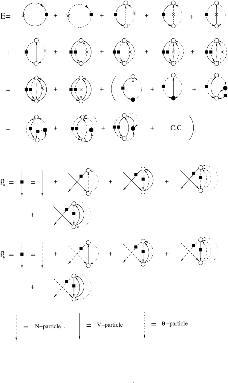
Figure 3.2: The symbols $\times$ and $\circ$ stand for kinetic energy and different parameters of wave function($C,C^{\prime},D,F,F^{\prime}$), respectively. The symbol $\bullet$ denotes the interaction coupling $W$. The out-going arrows form $\circ$ denote $V,N,\theta$-particle and in-coming arrows denote $V,N$-hole and $\bar{\theta}$-particle. The abbreviation C.C implies the complex conjugate terms.

The expectation value of the Hamiltonian is then obtained by and shown in Fig. 3.2

$$E=\frac{\langle\psi|H|\psi\rangle}{\langle\psi|\psi\rangle}=\sum_{a}h_{a}\rho_{a}+\sum_{b}h_{b}\rho_{b}+\sum_{ab}h_{ab}\rho_{a}\rho_{b},$$ (3.17)

where the Hamiltonian cluster integrals have been introduced as

$$h_{a}=\langle\psi_{a}|H|\psi_{a}\rangle,$$

$$h_{b}=\langle\psi_{b}|H|\psi_{b}\rangle,$$

$$h_{ab}=\langle\psi_{ab}|H|\psi_{ab}\rangle-h_{a}n_{b}-h_{b}n_{a},\$$ (3.18)

here $n_{a}$ and $n_{b}$ are the norm of $|\psi_{a}\rangle$ and $|\psi_{b}\rangle$ respectively. We disregard the other cluster integrals like $h_{aa^{\prime}}$ because they would only get contributions from two-mesons intermediate states. This makes sense in consistent one-meson exchange approximation. According to the selective summation made in the expression Eq. (3.17), the occupation numbers $\rho_{a}$ and $\rho_{b}$ should satisfy the following algebraic equations:

$$n_{a}\rho_{a}+\sum_{b}n_{ab}\rho_{a}\rho_{b}=1,$$

$$n_{b}\rho_{b}+\sum_{a}n_{ab}\rho_{b}\rho_{a}=1,\$$ (3.19)

with notation,

$$n_{ab}=\langle\psi_{ab}|\psi_{ab}\rangle-n_{a}n_{b}.$$ (3.20)

The basic idea for the treatment of $\langle\psi|H|\psi\rangle/\langle\psi|\psi\rangle$ is to expand it term by term using the Wick-rule to keep track of all possible contribution. The expansion of $\langle\psi|H|\psi\rangle$ and $\langle\psi|\psi\rangle$ can therefore be characterized by a set of suitable diagrams and one can check that the division by $\langle\psi|\psi\rangle$ cancels out all contribution from disconnected diagrams (the linked-cluster theorem). Now we minimize the quantity $E$ with respect to the constrains given by Eq. (3.3) and denote it $\overline{E}$, thus we multiply Eq. (3.3) by the Lagrange multipliers $\epsilon_{a}$ and $\epsilon_{b}$ and subtract them from Eq. (3.17), then by using the definition Eq. (3.3) we find

$$\overline{E} = \sum_{a}\rho_{a}(E_{a}^{0}-\epsilon_{a})+\sum_{b}\rho_{b}(E_{b}^{0}-\epsilon_{b})+\sum_{a}\rho_{a}\langle a|R_{1}^{{\dagger}}(H_{0}^{0}-\epsilon_{a})R_{1}$$ (3.21)

$$+R_{1}^{{\dagger}}H^{0}_{I}+H^{0}_{I}R_{1}|a\rangle+\sum_{b}\rho_{b}\langle b|R_{2}^{{\dagger}}(H_{0}^{0}-\epsilon_{b})R_{2}+R_{2}^{{\dagger}}H^{0}_{I}+H^{0}_{I}R_{2}|b\rangle$$

$$+\sum_{ab}\rho_{b}\rho_{a}\langle ba|S^{{\dagger}}(H_{0}^{0}-\epsilon_{a}-\epsilon_{b})S+R_{3}^{{\dagger}}(H_{0}^{0}-\epsilon_{a}-\epsilon_{b})R_{3}$$

$$+R_{4}^{{\dagger}}(H_{0}^{0}-\epsilon_{a}-\epsilon_{b})R_{4}+S^{{\dagger}}H^{0}_{I}R+R^{{\dagger}}H^{0}_{I}S|ab\rangle.\$$

It is convenient to treat the $\rho_{a}$ and $\rho_{b}$ as independent variables, therefore we minimize $\overline{E}$ respect to $R^{*}_{aBk},R^{*}_{Abk^{\prime}},S^{*}_{ABab},R^{*}_{BB^{\prime}abk},R^{*}_{AA^{\prime}abk},\rho_{a}$,$\rho_{b}$ which respectively yields:

$$R_{aBk}(E_{B}^{0}+\omega_{k}-\epsilon_{a})+W_{aBk}^{0*}+\sum_{Ab}\rho_{b}S_{ABab}W_{Abk}^{0*}=0,$$ (3.22)

$$R_{Abk^{\prime}}(E_{A}^{0}+\omega_{k^{\prime}}-\epsilon_{b})+W_{Abk^{\prime}}^{0*}+\sum_{Ba}\rho_{a}S_{ABab}W_{aBk^{\prime}}^{0*}=0,$$ (3.23)

$$\langle AB|(H_{0}^{0}-\epsilon_{a}-\epsilon_{b})S+H^{0}_{I}R|ab\rangle=0,$$ (3.24)

$$\langle BB^{\prime}k|(H_{0}^{0}-\epsilon_{a}-\epsilon_{b})R_{3}+H^{0}_{I}S|ab\rangle=0,$$ (3.25)

$$\langle AA^{\prime}k^{\prime}|(H_{0}^{0}-\epsilon_{a}-\epsilon_{b})R_{4}+H^{0}_{I}S|ab\rangle=0,$$ (3.26)

$$\epsilon_{a}=E_{a}^{0}+\langle a|R_{1}^{{\dagger}}(H_{0}^{0}-\epsilon_{a})R_{1}+R_{1}^{{\dagger}}H^{0}_{I}+H^{0}_{I}R_{1}|a\rangle+\sum_{b}\rho_{b}\langle ab|(R_{1}^{{\dagger}}+R_{2}^{{\dagger}})H^{0}_{I}S|ab\rangle,$$

$$\epsilon_{b}=E_{b}^{0}+\langle b|R_{2}^{{\dagger}}(H_{0}^{0}-\epsilon_{b})R_{2}+R_{2}^{{\dagger}}H^{0}_{I}+H^{0}_{I}R_{2}|b\rangle+\sum_{a}\rho_{a}\langle ab|(R_{1}^{{\dagger}}+R_{2}^{{\dagger}})H^{0}_{I}S|ab\rangle.$$

Equations (3.22)-(3.3) represent a set of unrenormalized Variational coupled integral equations for $N-V$ matter, consistent with two-hole-line truncation.

3.4 The renormalized nuclear matter equations

The method that we will use to reformulate Eqs. (3.22)-(3.3) in order to obtain renormalized equations for $N-V$ matter is based on the Feshbach projection operator formalism [56]. Projection operator techniques have also been used to analyze several sectors of the Lee model [77].

The total energy of $N-V$ matter can be obtained by making use of Eq. (3.21) and Eqs. (3.24)-(3.3) and exploiting the constrains Eq. (3.3);

$$E=\sum_{a}\epsilon_{a}+\sum_{b}\epsilon_{b}-\sum_{ab}\rho_{a}\rho_{b}\langle ab|(R_{1}^{{\dagger}}+R_{2}^{{\dagger}})H^{0}_{I}S|ab\rangle.$$ (3.28)

We can now directly add mass counter terms to the bare Hamiltonian in Eqs. (3.22) and (3.23) to dress masses. We expand the last term in the binding energy Eq. (3.28) in terms of the coupling constants and $S$. This form will be used later to achieve full renormalization for the binding energy since there is a subtle relation between $S$ and the renormalized coupling constant,

$$E = \sum_{a}\epsilon_{a}+\sum_{b}\epsilon_{b}-\sum_{abk^{\prime}AB}\rho_{a}\rho_{b}\frac{W^{0*}_{aBk^{\prime}}W^{0}_{Abk^{\prime}}}{\epsilon_{b}-E_{A}-\omega_{k^{\prime}}}S_{ABab}$$

$$- \sum_{abkAB}\rho_{a}\rho_{b}\frac{W^{0*}_{Abk}W^{0}_{aBk}}{\epsilon_{a}-E_{B}-\omega_{k}}S_{ABab}-\sum_{aa^{\prime}bk^{\prime}ABB^{\prime}}\rho_{a}\rho_{b}\rho_{a^{\prime}}\frac{W^{0*}_{aBk^{\prime}}W^{0}_{a^{\prime}B^{\prime}k^{\prime}}}{\epsilon_{b}-E_{A}-\omega_{k^{\prime}}}S^{*}_{AB^{\prime}a^{\prime}b}S_{ABab}$$

$$- \sum_{abb^{\prime}kAA^{\prime}B}\rho_{a}\rho_{b}\rho_{b^{\prime}}\frac{W^{0*}_{Abk}W^{0}_{A^{\prime}b^{\prime}k}}{\epsilon_{a}-E_{B}-\omega_{k}}S^{*}_{A^{\prime}Bab^{\prime}}S_{ABab}.\$$

The last two terms in Eq. (3.4) are a three-hole-line contribution which we ignore, consistent with our aim for a two-hole-line expansion. We introduce the projection operators

$$Q=\sum|AB\rangle\langle AB|,\hskip 42.67912ptQ^{\prime}=1/2\sum|BB^{\prime}k\rangle\langle BB^{\prime}k|,$$ (3.30)

$$Q^{\prime\prime}=1/2\sum|AA^{\prime}k^{\prime}\rangle\langle AA^{\prime}k^{\prime}|.$$

Inspired by the projection technique of feshbach, one can use the above definition to combine Eqs. (3.24)-(3.26),

$$\Big{[}H_{0}^{0}-z+QH^{0}_{I}\Big{(}Q^{\prime}\frac{1}{z-H_{0}^{0}}Q^{\prime}+Q^{\prime\prime}\frac{1}{z-H_{0}^{0}}Q^{\prime\prime}\Big{)}H^{0}_{I}Q\Big{]}S|ab\rangle=-QH^{0}_{I}(R_{1}+R_{2})|ab\rangle,$$ (3.31)

where $z=\epsilon_{a}+\epsilon_{b}$. We can show that the right hand side of Eq. (3.31) can be reduced by using Eqs. (3.22) and (3.23)

$$\langle AB|H^{0}_{I}R_{1}|ab\rangle=\sum_{k}W^{0}_{Abk}R_{aBk}$$

$$=\sum_{k}\frac{W^{0}_{Abk}W^{0*}_{aBk}}{\epsilon_{a}-E_{B}-\omega_{k}}-\sum_{b^{\prime}A^{\prime}k}\rho_{b^{\prime}}\frac{S_{A^{\prime}Bab}W^{0}_{Abk}W^{0*}_{A^{\prime}b^{\prime}k}}{\epsilon_{a}-E_{B}-\omega_{k}},$$ (3.32)

$$\langle AB|H^{0}_{I}R_{2}|ab\rangle=\sum_{k^{\prime}}W^{0}_{aBk^{\prime}}R_{Abk^{\prime}}$$

$$=\sum_{k^{\prime}}\frac{W^{0}_{aBk^{\prime}}W^{0*}_{Abk^{\prime}}}{\epsilon_{b}-E_{A}-\omega_{k^{\prime}}}-\sum_{a^{\prime}B^{\prime}k^{\prime}}\rho_{a^{\prime}}\frac{S_{AB^{\prime}ab}W^{0}_{aBk^{\prime}}W^{0*}_{a^{\prime}B^{\prime}k^{\prime}}}{\epsilon_{b}-E_{A}-\omega_{k^{\prime}}}.\$$ (3.33)

The second term in Eqs. (3.4) and (3.4) are a three-hole-line contribution which are again ignoreable in our approximation. Let us introduce the unrenormalized effective interaction $\overline{U}(z)$

$$\langle\alpha\beta|\overline{U}(z)|\alpha^{{}^{\prime}}\beta^{{}^{\prime}}\rangle=\langle\alpha\beta|H^{0}_{I}\frac{1}{z-\overline{H}_{0}}H^{0}_{I}|\alpha^{{}^{\prime}}\beta^{{}^{\prime}}\rangle_{\text{linked}}$$

$$=-\sum_{k}\frac{W^{0*}_{\alpha\beta^{{}^{\prime}}k}W^{0}_{\alpha^{{}^{\prime}}\beta k}}{z-\epsilon_{\beta}-\epsilon_{\beta^{{}^{\prime}}}-\omega_{k}}-\sum_{k^{\prime}}\frac{W^{0}_{\alpha\beta^{{}^{\prime}}k^{\prime}}W^{0*}_{\alpha^{{}^{\prime}}\beta k^{\prime}}}{z-\epsilon_{\alpha}-\epsilon_{\alpha^{{}^{\prime}}}-\omega_{k^{\prime}}},$$

$$\overline{H}_{0}=\sum_{\alpha}\epsilon_{\alpha}V^{{\dagger}}_{\alpha}V_{\alpha}+\sum_{\beta}\epsilon_{\beta}V^{{\dagger}}_{\beta}V_{\beta}+\sum_{k}\omega_{k}(a_{k}^{{\dagger}}a_{k}+b_{k}^{{\dagger}}b_{k}).\$$ (3.34)

The mass renormalization terms has been taken into account by using renormalized masses in the propagators. (Notice that $\epsilon_{A}=E_{A}$ and $\epsilon_{B}=E_{B}$). This definition correspondences to the quasi-potential in a Lippmann-Schwinger type equation if one replaces $H_{0}\to\overline{H}_{0}$. Having made use of defined effective interaction $\overline{U}(z)$ one can show

$$\langle AB|H^{0}_{I}(R_{1}+R_{2})|ab\rangle\simeq\langle AB|\overline{U}(z)|ab\rangle.$$ (3.35)

This expression is consistent with the two-hole-line approximation. Now we decompose the “p-p” and “n-n” interaction involved in Eq. (3.31) after adding mass counter terms in bare Hamiltonian,

$$QH^{0}_{I}\big{(}Q^{\prime}\frac{1}{z-H_{0}}Q^{\prime}+Q^{\prime\prime}\frac{1}{z-H_{0}}Q^{\prime\prime}\big{)}H^{0}_{I}Q=Q\overline{U}(z)Q+h(z)+\overline{q}(z),$$ (3.36)

where the operator $h(z)$ and $\overline{q}(z)$ are defined via Eqs. (3.2,3.2) as

$$h(z)|AB\rangle=[h_{A}(z-E_{B})+h_{B}(z-E_{A})]|AB\rangle,$$ (3.37)

$$\overline{q}(z)|AB\rangle=-\Big{(}\sum_{bk}\frac{|W^{0}_{Abk}|^{2}}{z-E_{b}-E_{B}-\omega_{k}}+\sum_{ak^{\prime}}\frac{|W^{0}_{aBk^{\prime}}|^{2}}{z-E_{a}-E_{A}-\omega_{k^{\prime}}}\Big{)}|AB\rangle.\$$

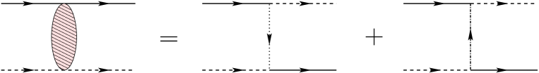
Figure 3.3: The effective two-body interaction, the lines are defined in Fig. 3.1.

In diagrammatic language Eq. (3.36) contains self-energy diagrams which contain unoccupied intermediate states because of the operators $Q^{\prime},Q^{\prime\prime}$, This is achieved by adding $\overline{q}(z)$ to $h(z)$. We now introduce the operator $B(z)$ to accomplish coupling constant renormalization. Its structure emerges from renormalization of finite sectors of ELM,

$$B(z)|\alpha\beta\rangle=Z^{2}_{\alpha}(z-E_{\beta})Z^{2}_{\beta}(z-E_{\alpha})|\alpha\beta\rangle,$$ (3.38)

with notations,

$$Z^{2}_{\alpha}(z)=1+\sum_{\beta k}\frac{|W^{0}_{\alpha\beta k}|^{2}}{(E_{\alpha}-E^{0}_{\beta}-\omega_{k})(z-E^{0}_{\beta}-\omega_{k^{\prime}})},$$

$$Z^{2}_{\beta}(z)=1+\sum_{\alpha k^{\prime}}\frac{|W^{0}_{\alpha\beta k^{\prime}}|^{2}}{(E_{\beta}-E^{0}_{\alpha}-\omega_{k^{\prime}})(z-E^{0}_{\alpha}-\omega_{k^{\prime}})},\$$ (3.39)

here $z=E_{\alpha}+E_{\beta}$. The benefit of $B(z)$ can be manifested by following factorization property

$$Q(z-H_{0}^{0}-h(z))Q=Q(z-H_{0})B(z)Q.$$ (3.40)

One may use $B(z)$ to show that $\overline{U}(z)$ is related to renormalized effective $N-V$ potential

$$U(z)=B(z)^{1/2}\overline{U}(z)B(z)^{1/2}.$$ (3.41)

Therefore, the renormalized effective two-body $N-V$ potential can be readily found ( see Fig. 3.2)

$$\langle\alpha\beta|U(z)|\alpha^{{}^{\prime}}\beta^{{}^{\prime}}\rangle=-\sum_{k}\frac{r_{\alpha}(z-E_{\beta})r_{\beta}(z-E_{\alpha})W^{*}_{\alpha\beta^{{}^{\prime}}k}W_{\alpha^{{}^{\prime}}\beta k}r_{\alpha^{{}^{\prime}}}(z-E_{\beta^{{}^{\prime}}})r_{\beta^{{}^{\prime}}}(z-E_{\alpha^{{}^{\prime}}})}{z-\epsilon_{\beta}-\epsilon_{\beta^{{}^{\prime}}}-\omega_{k}}$$

$$-\sum_{k^{\prime}}\frac{r_{\alpha}(z-E_{\beta})r_{\beta}(z-E_{\alpha})W_{\alpha\beta^{{}^{\prime}}k^{\prime}}W^{*}_{\alpha^{{}^{\prime}}\beta k^{\prime}}r_{\alpha^{{}^{\prime}}}(z-E_{\beta^{{}^{\prime}}})r_{\beta^{{}^{\prime}}}(z-E_{\alpha^{{}^{\prime}}})}{z-\epsilon_{\alpha}-\epsilon_{\alpha^{{}^{\prime}}}-\omega_{k^{\prime}}},$$ (3.42)

where we have introduced twice-subtracted “dressing factor” defining as

$$r_{\alpha}(z)=\frac{Z_{\alpha}(E_{\alpha})}{Z_{\alpha}(z)},\hskip 56.9055ptr_{\beta}(z)=\frac{Z_{\beta}(E_{\beta})}{Z_{\beta}(z)}.$$ (3.43)

Dressing factor appears independent of truncation made and describes off shell correction of a self-energy of $V$ and $N$ particle. In Lee model $r_{\beta}(z)=1$, since $N$-particle stay unrenormalized. Twice-subtracted dressing factors remain finite even without form factor, due to the occurrence of a cubic energy denominator, this can be verified by expanding Eq. (3.43) using relativistic expression for $E_{\alpha},E_{\beta},\omega_{k},\omega_{k^{\prime}}$ and interaction strength. Now one can rewrite Eq. (3.31), by making use of Eqs. (3.35, 3.36) and exploiting the factorization property Eq. (3.40)

$$\big{(}H_{0}-z+q(z)+U(z)\big{)}B(z)^{1/2}S|ab\rangle=-QU(z)B(z)^{1/2}|ab\rangle,$$ (3.44)

where $q(z)$ is renormalized two-body operators obtained from Eq. (3.37)

$$q(z)|AB\rangle =-\Big{(}\sum_{bk}\frac{|W_{Abk}|^{2}r^{2}_{A}(z-E_{B})r^{2}_{B}(z-E_{A})}{z-E_{b}-E_{B}-\omega_{k}}$$ (3.45)

$$+\sum_{ak^{\prime}}\frac{|W_{aBk^{\prime}}|^{2}r^{2}_{A}(z-E_{B})r^{2}_{B}(z-E_{A})}{z-E_{a}-E_{A}-\omega_{k^{\prime}}}\Big{)}|AB\rangle.\$$

It is observed the operator $B(z)$, transfers unrenormalized correlation function to renormalized one. This is due to the simple structure of vertices renormalization in this model. We now turn to Eq. (3.3) for $\epsilon_{a}$ and $\epsilon_{b}$, one may use Eqs. (3.22,3.23) to obtain

$$\epsilon_{a} = E^{0}_{a}+\sum_{Bk}R_{aBk}W^{0}_{aBk}+\sum_{bk^{\prime}AB}\rho_{b}R^{*}_{Abk^{\prime}}W^{0*}_{aBk^{\prime}}S_{ABab}$$

$$= E^{0}_{a}+\sum_{Bk}\frac{|W^{0}_{aBk}|^{2}}{\epsilon_{a}-E^{0}_{B}-\omega_{k}}+\sum_{bkAB}\rho_{b}\frac{W^{0}_{aBk}W^{0*}_{Abk}}{\epsilon_{a}-E^{0}_{B}-\omega_{k}}S_{ABab}$$

$$+ \sum_{bk^{\prime}AB}\rho_{b}\frac{W^{0*}_{aBk^{\prime}}W^{0}_{Abk^{\prime}}}{\epsilon_{b}-E^{0}_{A}-\omega_{k^{\prime}}}S_{ABab}+\sum_{a^{\prime}bk^{\prime}ABB^{\prime}}\rho_{b}\rho_{a^{\prime}}\frac{W^{0*}_{aBk^{\prime}}W^{0}_{a^{\prime}B^{\prime}k^{\prime}}}{\epsilon_{b}-E^{0}_{A}-\omega_{k^{\prime}}}S^{*}_{AB^{\prime}a^{\prime}b}S_{ABab},$$

$$\epsilon_{b} = E^{0}_{b}+\sum_{Ak^{\prime}}R_{Abk^{\prime}}W^{0}_{Abk^{\prime}}+\sum_{akAB}\rho_{a}R^{*}_{aBk}W^{0*}_{bAk}S_{ABab}$$

$$= E^{0}_{b}+\sum_{Ak^{\prime}}\frac{|W^{0}_{Abk^{\prime}}|^{2}}{\epsilon_{b}-E^{0}_{A}-\omega_{k^{\prime}}}+\sum_{ak^{\prime}AB}\rho_{a}\frac{W^{0}_{Abk^{\prime}}W^{0*}_{aBk^{\prime}}}{\epsilon_{b}-E^{0}_{A}-\omega_{k^{\prime}}}S_{ABab}$$

$$+ \sum_{bkAB}\rho_{a}\frac{W^{0*}_{bAk}W^{0}_{aBk}}{\epsilon_{a}-E^{0}_{B}-\omega_{k}}S_{ABab}+\sum_{ab^{\prime}kA^{\prime}AB}\rho_{a}\rho_{b^{\prime}}\frac{W^{0*}_{Abk}W^{0}_{A^{\prime}b^{\prime}k}}{\epsilon_{a}-E^{0}_{B}-\omega_{k}}S^{*}_{A^{\prime}Bab^{\prime}}S_{ABab}.$$

The last term in $\epsilon_{a}(\epsilon_{b})$ in Eq. (3.4) are a three-hole-line contribution. From Eqs. (3.2) and (3.2) it is obvious that the first two terms in $\epsilon_{a}(\epsilon_{b})$ in Eq. (3.4) are the renormalized energy of $N(V)$ particles if we add the contribution of intermediate occupied $a(b)$ states in self-energy. The corresponded terms should be subtracted which contribute to the definition of $\bar{\epsilon_{a}}(\bar{\epsilon_{b}})$. Having introduced mass counter terms, one can eliminate $S$ by using Eq. (3.44) and obtain the renormalized equation for $E$, $\epsilon_{a}$ and $\epsilon_{a}$,

$$E=\sum_{a}\epsilon_{a}+\sum_{b}\epsilon_{b}-\sum_{ab}\rho_{b}\rho_{a}\langle ab|G(\epsilon_{a}+\epsilon_{b})|ab\rangle+\sum_{ab}\rho_{a}\rho_{b}\langle ab|U(\epsilon_{a}+\epsilon_{b})|ab\rangle,$$

(3.47)

$$\epsilon_{a}=E_{a}+\bar{\epsilon_{a}}+\sum_{b}\rho_{b}\langle ab|G(\epsilon_{a}+\epsilon_{b})|ab\rangle,$$ (3.48)

$$\epsilon_{b}=E_{b}+\bar{\epsilon_{b}}+\sum_{a}\rho_{a}\langle ab|G(\epsilon_{a}+\epsilon_{b})|ab\rangle,$$ (3.49)

$$G(z)=U(z)+U(z)\frac{Q}{z-H_{0}-q(z)}G(z),$$ (3.50)

$$\bar{\epsilon_{a}}=-\sum_{bk}\frac{|W_{abk}|^{2}r^{2}_{a}(\epsilon_{a})r^{2}_{b}(\epsilon_{b})}{\epsilon_{a}-E_{b}-\omega_{k}}-\sum_{b}\rho_{b}\langle ab|U(\epsilon_{a}+\epsilon_{b})|ab\rangle,$$ (3.51)

$$\bar{\epsilon_{b}}=-\sum_{ak^{\prime}}\frac{|W_{abk^{\prime}}|^{2}r^{2}_{a}(\epsilon_{a})r^{2}_{b}(\epsilon_{b})}{\epsilon_{b}-E_{a}-\omega_{k^{\prime}}}-\sum_{a}\rho_{a}\langle ab|U(\epsilon_{a}+\epsilon_{b})|ab\rangle,\$$ (3.52)

where $\epsilon_{a}$ and $\epsilon_{b}$ are given by self-consistent equation of the Brueckner type and $G(z)$ is the solution of a Brueckner-Bethe-Goldstone equation [68, 78].

3.5 Conclusion

The correction to the standard many-body scheme emerges in this model in different steps which are connected with the following physical effects. We have to replace the $V^{OBE}$ by $U(z)$, which accounts for the renormalization effects of the boson propagating in the $N-V$ matter system. This can be understood since fermions feel the average potential given by $\epsilon_{a}$ and $\epsilon_{b}$ during the time when a boson is exchanged in $N-V$ matter [78]. In scattering formalism ($T$-matrix) we have $z=E_{\alpha}+E_{\beta}$, the total energy of $N-V$ system, whereas there is a medium effect in $N-V$ matter bringing the $z$-value to $z=\epsilon_{a}+\epsilon_{b}$. The energy denominator of the Brueckner Eq. (3.50) contains the correction $q(z)$ which is not present for standard $N-V$ scattering. This correction is due to the effect of the Pauli principle on the self-energy of the fermions. The comparison between many-body solution in the Lee model [72] and the ELM reveals following distinctions:
The simplest correction in the ELM is due to the self-energy diagrams of $N$-particle and Pauli principle on this diagrams which are manifested through the occurrence of the corresponding dressing factor $r_{\beta}(z)$ and $q(z)$ respectively, whereas these corrections in the Lee model do not appear because $N$-particle remains unrenormalized . In the Lee model the lowest order of $\epsilon_{b}$ would appear in a three-hole-line expansion while in the ELM this term arises in two-hole-line contribution on an equal footing with lowest order of $\epsilon_{a}$.

Figure 3.4: The symbol $\times$ stands for the renormalization counter term which is shown on the left land side.

The $\rho_{b}$ renormalization correction of the Lee model (see Fig. 3.4) goes to contribution of mass renormalization of $N$-particle in the ELM. Therefore the renormalization correction of occupation numbers gets contribution from higher order which are not generated in our approximation. It is notable that the ELM due to possessing the crossing symmetry preserves the symmetry between $V$ and $N$ part of the renormalization correction, whereas this is not the case for many-body problem within Lee model.

This presentation is conclusive that coupled-cluster theory without the decoupling property in systematic truncation scheme leads to derivation of generalized Brueckner ($E$-dependent) theory which includes renormalization correction originating from medium effect. We showed as well that a combination of the coupled-cluster theory and Feshbach projection technique provides a powerful method to renormalize quantum many-body problem in a truncated Fock space.

3.6 Some final remarks

We have employed the coupled-cluster theory in various versions and investigated the merits and short-comings of such techniques for field theoretical applications. We showed that the CCM version introduced by Arponen and Bishop can be easily adopted with Wilsonian renormalization group and provides very strong tools for describing (non)-perturbative phenomena (please see the conclusion of the last chapter 2.11). On the other hand, the CCM version introduced by Schütte and Providencia can be equipped with the Feshbach projection formalism and produces a renormalized generalized Brueckner theory. One should bear in mind that in the latter, the famous “small-energy denominator” problem is not avoidable and is not at all clear how systematically high-energy modes can be integrated out for a very complicated system.

In the rest of this work, we employ an effective QCD model as can be constructed from the techniques of the first part of this thesis and address with greater details, non-perturbative phenomenological phenomena such as nucleon and diquark solutions, confinement and spontaneous chiral symmetry breaking.

Chapter 4 QCD properties and effective quark chiral models

It is believed that the strong interactions are described by a quantum field theory known as quantum chromodynamics (QCD) [50, 79]. QCD from many aspects is an unique theory. Quantum electrodynamics (QED), and its expansion to the electroweak standard model of particle physics, is also a quantum field theory. However, QED breaks down at short distances and is not well-defined. QED is renormalizable theory but it loses all his credibility as we approach to Landau pole. On the other hand if the cutoff goes to infinity, QED becomes trivial. QED is not the only theory with a Landau pole problem, every theory which is not asymptotically free suffers from this problem. The quantum field theory of gravity obtained from general relativity suffers from nonrenormalizability. QCD is the only known theory which is free from such problems. QCD only needs few parameters to be defined completely, one universal coupling strength and one mass for each kind of quark.

In following chapter we introduce part of QCD which is relevant to nuclear physics. We refrain from discussing all details since it can be found in many quantum-field theory textbooks, see e.g., Refs. [50, 79].

4.1 QCD Symmetries

In this section we will introduce the underlying symmetries of QCD. The Lagrangian of QCD is given by [50, 79],

$$\mathcal{L}=\bar{q}(i\gamma^{\mu}\partial_{\mu}-m^{0})q-\frac{1}{4}(F^{a}_{\mu\nu})^{2}+g\bar{q}\gamma^{\mu}A_{\mu}q,$$ (4.1)

where $q$ is the quark field which is defined in the fundamental representation of the color and flavor group, and the conjugate Dirac field is defined as $\bar{q}=q^{{\dagger}}\gamma^{0}$. The gluon field matrix $A^{\mu}=A^{a}_{\mu}\lambda^{a}/2$ is defined in the fundamental $SU(N_{c}=3)$ representation, $\lambda^{a}$ being the generators of the gauge group which satisfies $[\lambda^{a}/2,\lambda^{b}/2]=if^{abc}\lambda^{c}/2$. We define $g$ as strong coupling constant. The field strength $F^{a}_{\mu\nu}$ is given by

$$F^{a}_{\mu\nu}=\partial_{\mu}A^{a}_{\nu}-\partial_{\nu}A^{a}_{\mu}+gf^{abc}A^{b}_{\mu}A^{c}_{\mu}.$$ (4.2)

The non-Abelian nature of QCD is manifested by the quadratic term in the gauge field strength. The color and flavour indices of the quark field are suppressed. $m^{0}$ is the current quark mass which is not directly observable if QCD confines quarks. The current quark mass is color-independent and can be brought diagonal in flavour space. There are six flavours of quarks, each of which has a different mass. The three light quarks are called up (u), down (d) and strange (s), while the three heavy quarks are called charm (c), bottom (b) and top (t). The following values for the light current quark masses are found from the Particle Data group [80],

$$m^{0}_{u}=2~{}~{}\text{to}~{}~{}8~{}~{}\text{MeV},\hskip 28.45274ptm^{0}_{d}=5~{}~{}\text{to}~{}~{}15~{}~{}\text{MeV},\hskip 28.45274ptm^{0}_{s}=100~{}~{}\text{to}~{}~{}300~{}~{}\text{MeV}.$$ (4.3)

Notice that the quark masses are renormalization-scheme dependent. The above values are obtained in a subtraction scheme at a renormalization scale $\mathcal{O}(1\text{GeV})$. In addition to flavour, quarks carry another quantum number known as colour. Each quark comes in three colours, red, green and blue.

The Lagrangian Eq. (4.1) has a large classical symmetry: we have the local gauge symmetry $SU(N_{c})$ by construction,

$$q\to U_{c}q,\hskip 56.9055pt\bar{q}\to\bar{q}U^{{\dagger}}_{c},\hskip 56.9055ptU_{c}(x)=\exp(i\theta^{a}(x)(\frac{\lambda^{a}}{2})_{c}),$$

$$A_{\mu}\to U_{c}A_{\mu}U^{{\dagger}}_{c}-\frac{1}{g}U_{c}i\partial_{\mu}U^{{\dagger}}_{c}.\$$

We have also global flavour symmetry which does not affect the gluon fields,

$$q\to U_{V}q,\hskip 56.9055pt\bar{q}\to\bar{q}U^{{\dagger}}_{V},\hskip 56.9055ptU_{V}=\exp(i\theta^{a}_{V}(\frac{\lambda^{a}}{2})_{F}).$$ (4.4)

where $(\frac{\lambda^{a}}{2})_{F}$ denotes the generators of the flavor group $U(N_{f})$ and $N_{f}$ denotes the number of flavors. The above symmetry is referred to as vector flavor symmetry $U_{V}(N_{f})$. When the generator matrix is taken unit matrix we have $U_{V}(1)$ symmetry associated with conservation of baryon number. There is another global symmetry which is exact at $m^{0}=0$, namely chiral symmetry. This symmetry is very similar to vector flavor symmetry, apart from an extra factor of $\gamma_{5}$ in the generator of the transformation.

$$q\to U_{A}q,\hskip 56.9055pt\bar{q}\to\bar{q}U_{A},\hskip 56.9055ptU_{A}=\exp\left(i\gamma_{5}\theta_{A}^{a}(\frac{\lambda^{a}}{2})_{F}\right).$$ (4.5)

Notice that due to the factor $\gamma_{5}$ the quark field and its conjugate partner are transformed by the same matrix in contrast to vector transformation Eq. (4.4). This transformation is called the axial-vector transformation and can be combined with the vector transformation to define a bigger symmetry at chiral $m^{0}=0$ which is then called chiral symmetry $U_{V}(N_{f})\times U_{A}(N_{f})$. One may alternatively define right- and left-handed quark fields by following transformation

$$q_{L}=\frac{1-\gamma_{5}}{2}q,\hskip 56.9055ptq_{R}=\frac{1+\gamma_{5}}{2}q,$$ (4.6)

The right- and left-handed massless fermions are eigenvalues of the helicity or chirality (with eigenvalue $\pm 1$) and are not mixed together. The chiral symmetry can be equivalently written as $U_{L}(N_{f})\times U_{R}(N_{f})$.

It is believed that intermediate-energy hadronic physics, say over range of energy MeV-GeV is adequately described by the dynamics of the lowest-mass quarks, $u$ and $d$. The overall classical symmetry of the Lagrangian with $N_{f}=2$ becomes

$$SU(N_{c})_{\text{local}}\times(SU(2)_{L}\times SU(2)_{R}\times U(1)_{V}\times U(1)_{A})_{\text{global}},$$ (4.7)

Not all above-mentioned symmetries survive quantization. Particles with opposite helicity are related by a parity transformation, therefore in a chirally symmetric world the hadrons should come in parity doublets. However, in a real life we do not observe such degeneracy. Therefore, one can conclude that chiral symmetry is not realized in the ground state and chiral symmetry is spontaneously broken. The Goldstone theorem tell us that the spontaneous breaking of a continuous global symmetry implies the existence of associated massless spinless particles. This indeed confirmed due to the existence of the light pseudoscalar mesons in nature (pions, kaons and etas) as the corresponding Goldstone bosons [81]. Moreover, the existence of quark condensate $\langle\bar{q}q\rangle$ implies that the $SU(N_{f})_{L}\times SU(N_{f})_{R}$ symmetry is spontaneously broken down to $SU(N_{f})_{V}$. Therefore one may conceive QCD quark condensate as an order parameter for chiral symmetry breaking. The concept of spontaneous broken chiral symmetry is the cornerstone in the understanding of the low-energy hadronic spectrum.

The $U(1)_{A}$ symmetry implies that all hadrons should come with opposite parity partners. However, this is not the case, therefore this symmetry must be broken somehow. If the spontaneous symmetry breaking mechanism works here, then one should observe Goldstone boson associated with $U(1)_{A}$, namely an $I=0$ pseudoscalar meson having roughly the same mass as the pion. Surprisingly there is no such Goldstone boson. This problem is sometime called $U(1)_{A}$ puzzle. It turned out that the $U(1)_{A}$ symmetry is explicitly broken by quantum effects. This effect is known as the axial anomaly [82]. It was shown by ’t Hoof that due to instanton effects, the $U(1)_{A}$ symmetry is not manifested in nature [82].

Finally, at $m^{0}=0$, the QCD Lagrangian is invariant under a scale transformation which is called dilatational symmetry:

$$q(x)\to\epsilon^{3/2}q(\epsilon^{-1}x),\hskip 56.9055ptA^{a}_{\mu}(x)\to\epsilon A^{a}_{\mu}(\epsilon^{-1}x),\hskip 56.9055ptx_{\mu}\to\epsilon^{-1}x_{\mu}.$$ (4.8)

This symmetry is again broken at quantum level due to the trace anomaly [83].

4.2 Non-perturbative features of QCD

In this section we shall recapitulate the most important features of QCD which are not accessible perturbatively. Let us firstly elaborate why perturbation theory in terms of coupling $g$ can not be used in the low-energy regime of the theory. Having introduced the gauge fixing term and an associated ghost term by means of the Faddeev-Popv procedure [50, 79, 84], one can carry out perturbation theory in terms of coupling. Due to the renormalization process, a renormalization scale $\mu$ enters the algebra [85]. Therefore the running coupling is described by the RG equation

$$\frac{dg(\mu)}{d\ln\mu}=\beta(g).$$ (4.9)

Where the coupling is small, the $\beta$ function can be computed perturbatively,

$$\beta(g)=-\frac{\beta_{0}}{(4\pi)^{2}}g^{3}-\frac{\beta_{1}}{(4\pi)^{4}}g^{5}+...,$$ (4.10)

with

$$\beta_{0}=11-\frac{2}{3}N_{f},\hskip 56.9055pt\beta_{1}=102-\frac{38}{3}N_{f}.$$ (4.11)

Therefore, one can readily calculate the effective running coupling

$$\alpha_{s}(\mu)=\frac{g^{2}(\mu)}{4\pi}=\frac{12\pi}{(33-2N_{f})\ln(\mu^{2}/\Lambda^{2})}\times[1-\frac{(918-114N_{f})\ln(\ln(\mu^{2}/\Lambda^{2}))}{(33-2N_{f})^{2}\ln(\mu^{2}/\Lambda^{2})}],$$ (4.12)

where $\Lambda$ is a scale parameter of QCD and depends on the subtraction scheme and the number of active flavours,

$$\Lambda_{\overline{MS}}^{(5)}=(208^{+25}_{-23})\text{MeV},$$ (4.13)

where the symbol $\overline{MS}$ stands for minimal subtraction scheme [79] and the superscripts indicate the number of active flavours. This value is taken from an analysis of the various high energy processes, see Ref. [86]. The most striking feature of the running coupling is that it decreases logarithmically as $\mu$ increases. Therefore perturbation theory works very well for large $\mu$. This phenomenon is called asymptotic freedom [87]. However, if $\mu$ is near $\Lambda_{\overline{MS}}$, perturbation theory does not work anymore and non-perturbative phenomena enter the stage. Admittedly, there is no unambiguous method available to connect small and large distances in QCD.

One of the most important non-perturbative features of QCD is dynamical chiral symmetry breaking which is responsible for generation of a quark mass from nothing. In order to show that this phenomenon is purely non-perturbative, we employ the QCD gap equation [90],

$$S(p)^{-1}=(i\gamma.p+m^{0})+\int\frac{d^{4}q}{(2\pi)^{4}}g^{2}D_{\mu\nu}(p-q)\frac{\lambda^{a}}{2}\gamma_{\mu}S(q)\Gamma^{a}_{\nu}(p,q),$$ (4.14)

where $m^{0}$ and $g$ are the current-quark bare mass and the coupling constant, respectively. $D_{\mu\nu}(p-q)$ is the dressed-gluon propagator and $\Gamma^{a}_{\nu}(p,q)$ is the dressed-quark-gluon vertex. The general solution of the gap equation is a dressed-quark propagator of the form

$$S(p)=\frac{1}{i\gamma.pA(p^{2})+B(p^{2})}=\frac{Z(p^{2})}{i\gamma.p+M(p^{2})}.$$ (4.15)

One may now use the gap equation to work out the fermion self-energy perturbatively [91]. One obtains,

$$B(p^{2})=m^{0}\left(1-\frac{\alpha}{\pi}\ln(p^{2}/m^{2})+...\right).$$ (4.16)

It is observed that at all orders of loop expansion terms are proportional to the current-quark mass and consequently vanish as $m^{0}\to 0$. Therefore, no mass (the quark mass is defined as a pole of the dressed-quark propagator) is generated at current-quark mass equal to zero, i.e. the dynamical chiral symmetry breaking is impossible in perturbation theory and there is no mixing between left- and right-handed quarks “perturbatively”. Notice that apart from the trivial solution $B(p^{2})=0$ at $m=0$, a non-trivial solution $B(p^{2})\neq 0$ can indeed be found at the chiral point, albeit accessible non-perturbatively. The renormalization effect is not included in Eq. (4.14), but it does not change the above argument [91]. As we already mentioned, there is a close relationship between the generation of the quark mass, $B(p^{2})\neq 0$, and the fact that $\langle\bar{q}q\rangle\neq 0$. The quark condensate in QCD is given by the trace of the full quark propagator Eq. (4.15),

$$\langle\bar{q}q\rangle=-i\lim_{y\to x}{\rm Tr}S(x,y).$$ (4.17)

Notice that since $\bar{q}q$ is a gauge invariant object, one may take any gauge to obtain the dressed quark propagator which has a general form as equation (4.15). It is obvious when we have $B(p^{2})=0$, never does the quark condensate take place, simply because of the identity ${\rm Tr}\gamma_{\mu}=0$. It has been shown in Landau gauge that the dynamical quark mass, $M(p^{2})$ is large in infrared, $M(0)\sim 0.5$ GeV, but is power-law suppressed in the ultraviolet [92],

$$M(p^{2})^{\text{large}-p^{2}}=\frac{2\pi^{2}\gamma_{m}}{3}\frac{-\langle\bar{q}q\rangle^{0}}{p^{2}\left(\frac{1}{2}\ln[\frac{p^{2}}{\Lambda_{QCD}}]\right)^{1-\gamma_{m}}},$$ (4.18)

where $\gamma_{m}=12/(33-2N_{f})$ is the mass anomalous dimension and $\langle\bar{q}q\rangle^{0}$ is the renormalization group invariant vacuum quark condensate. The dressed-quark mass-function Eq. (4.18) is a longstanding prediction of the Dyson-Schwinger equation [90] and has been recently confirmed by quenched lattice QCD [93]. It has been shown in many non-perturbative approaches that the emergence of a dynamical quark mass leads to the non-vanishing of quark condensate and vice versa, e.g., see chapter 6.

Another important non-perturbative feature of QCD is color confinement [94]. Loosely speaking, confinement is defined as the absence of any colored object in nature. But it is possible that there exists a composite colored particle which can form colorless bound states with another colored particle like quarks. The color confinement is still not properly understood, and a clear and indisputable mechanism responsible for this effect yet remains to be discovered . Confinement originates non-perturbatively, since it is associated with a linear potential with a string tension $\sigma\propto\Lambda^{2}e^{-\int\frac{dg}{\beta(g)}}$ which is obviously non-perturbative in the coupling.

One may wonder if there is a non-trivial solution for gap equation $B(p^{2})\neq 0$ which gives rise to a pole of the quark propagator, which would contradict QCD confinement since the quark is colored . Indeed this is one of the subtle point in every QCD model and can not be easily resolved. In principle, there will be a long-range force between massive quarks to confine them and also a short range spin-spin interaction between massive dressed quarks. The former will modify the low momentum part of the propagator to remove the quark from being on-shell. Actually, this describes a phenomenologically motivated picture of a constituent quark model based on the dynamical symmetry breaking. Having said that it is very hard to incorporate the dynamical symmetry breaking and the confinement into a QCD model. In fact, many models constructed to describe the low-energy properties of hadrons are assumed to be only dominated by the quark flavor dynamics and dynamical symmetry breaking and are indeed reliable only at intermediate scales, between confinement scale few hundred MeV up to a scale about 1 GeV.

4.3 Effective low-energy quark interaction

Physical hadrons are colorless objects and their properties seem to be determined by the flavor dynamics which is induced by an effective QCD interaction. The first step toward a construction of such effective theory is to integrate out gluonic degrees of freedom, then by standard bozonization and hadronization methods [95] derive the desired effective low-energy theories based on relevant degrees of freedom. There have been many attempts to attack this difficult problem. Two very well established methods are the global color model approach introduced by Cahill and Roberts [96], and the so-called field strength approach introduced by Reinhardt and collaborators [97]. Our main goal in this section is to give a taste of such approaches and focus only on the main themes rather than details. First we rewrite the quark-gluon interaction term in QCD Lagrangian Eq (4.1) by rewriting

$$\bar{q}\gamma^{\mu}A_{\mu}q=A^{a}_{\mu}J^{\mu}_{a},\hskip 56.9055ptJ^{\mu}_{a}=\bar{q}\frac{\lambda^{a}}{2}\gamma^{\mu}q.$$ (4.19)

The full quantum theory of QCD is solved by computing the functional integral describing the vacuum-to-vacuum transition amplitude,

$$Z_{QCD}=\int\mathcal{D}q\mathcal{D}\bar{q}\int\mathcal{D}A^{a}_{\mu}e^{i\int d^{4}x\mathcal{L}_{QCD}}.$$ (4.20)

In order to handle the gluonic part of the QCD functional integral, one first has to define gauge inequivalent orbits by using a standard gauge fixing procedure and the Faddeev-Popov method [50, 79] (in what follows we assume that this procedure has already been carried out). We now split the above generating functional integral as

$$Z_{QCD}=\int\mathcal{D}q\mathcal{D}\bar{q}\exp\left(i\int d^{4}x\bar{q}(i\gamma^{\mu}\partial_{\mu}-m^{0})q+\Gamma[J]\right),$$ (4.21)

where the gluon part of action is defined in

$$\Gamma[J]=\log\int\mathcal{D}A^{a}_{\mu}\exp\left(-\frac{1}{4}\int F^{2}+g\int A^{a}_{\mu}J^{\mu}_{a}\right).$$ (4.22)

If we could evaluate exactly the gluonic part of the functional integral then we would be done. But unfortunately this integration can not be handled unless we resort to some sort of systematic approximation (this is due to the presence of cubic and quartic terms of $A^{a}_{\mu}$ in the Lagrangian). One possibility to proceed is to expand the effective action in powers of the quark current $J^{a}_{\mu}$ as suggested by Cahill and Roberts [96],

$$\Gamma[J] = \Gamma[J=0]+g\int\Gamma^{(1)a}_{\mu}J^{\mu}_{a}dx_{1}+\frac{g^{2}}{2}\int\Gamma^{2}(x_{1},x_{2})^{a_{1}a_{2}}_{\mu_{1}\mu_{2}}J^{\mu_{1}}_{a_{1}}J^{\mu_{2}}_{a_{2}}dx_{1}dx_{2}+...$$ (4.23)

$$+ \frac{g^{n}}{n!}\int\Gamma^{(n)}(x_{1},x_{2},..x_{n})^{a_{1}..a_{n}}_{\mu_{1}...\mu_{n}}J^{\mu_{1}}_{a_{1}}...J^{\mu_{n}}_{a_{n}}dx_{1}...dx_{n},\$$

where the coefficients

$$\Gamma^{(n)}(x_{1},x_{2},...,x_{n})^{a_{1}...a_{n}}_{\mu_{1}...\mu_{n}}=\left(\frac{\partial^{n}\Gamma[J]}{\partial J^{a_{1}}_{\mu_{1}}..\partial J^{a_{n}}_{\mu_{n}}}\right)_{J=0},$$ (4.24)

are defined as one-particle irreducible gluon correlation functions in the absence of quarks,

$$\Gamma^{(1)}(x_{1})^{a_{1}}_{\mu_{1}} = \langle A^{a_{1}}_{\mu_{1}}(x_{1})\rangle,$$

$$\Gamma^{(2)}(x_{1},x_{2})^{a_{1},a_{2}}_{\mu_{1},\mu_{2}} = \langle A^{a_{1}}_{\mu_{1}}(x_{1})A^{a_{2}}_{\mu_{2}}(x_{2})\rangle-\langle A^{a_{1}}_{\mu_{1}}(x_{1})\rangle\langle A^{a_{2}}_{\mu_{2}}(x_{2})\rangle.\$$

In the above expression, the brackets denotes the functional average over the gluon field

$$\langle...\rangle=\frac{\int\mathcal{D}A...\exp\left(-\frac{1}{4}\int F^{2}\right)}{\int\mathcal{D}A\exp\left(-\frac{1}{4}\int F^{2}\right)}.$$ (4.25)

The zeroth order term $\Gamma[J=0]$ does not depend on the quark field and is therefore an irrelevant constant. The first order term $\Gamma^{(1)}$ gives the expectation value of the gluon field and is zero in the absence of external fields. The leading non-trivial term is $\Gamma^{2}(x_{1},x_{2})^{a_{1}a_{2}}_{\mu_{1}\mu_{2}}=D^{ab}_{\mu\nu}(x-y)$ which is the exact gluon propagator and includes all gluon self-interactions and gluon-ghost interactions. Notice that the quark loops are incorporated through the quark current attached as legs to the exact gluon propagator. The main approximation in this approach is to ignore all terms $n\geq 3$. Note that none of the gluon correlation functions is gauge or Lorentz invariant. While each term in the expansion is separately invariant under Lorentz and “global color symmetry”, nevertheless the whole expansion in Eq. (4.23) is invariant under local gauge symmetry. We truncate Eq. (4.23) up to $n=2$, and with this simplification the QCD generating functional is approximated by

$$Z_{QCD}\approx\int\mathcal{D}q\mathcal{D}\bar{q}\exp(iS_{QFD}),$$ (4.26)

where the $S_{QFD}$ is the induced non-local QCD action which describes the quark flavour dynamics,

$$S_{QFD}=\int\bar{q}(i\gamma^{\mu}\partial_{\mu}-m^{0})q+\frac{g^{2}}{2}\int\int\bar{q}(x)\gamma_{\mu}\frac{\lambda^{a}}{2}q(x)D(x-y)\bar{q}(y)\gamma_{\mu}\frac{\lambda^{a}}{2}q(y).$$ (4.27)

The exact form of $D(x)$ is not available at the moment. Hence, the main phenomenology task is to simulate the simplest form of gluon propagator in order to reproduce the confinement and asymptotic freedom of quarks. Although there is no a priori reason to believe that the effective interaction of quarks propagating in the QCD vacuum should retain the form of a one gluon exchange interaction, it has been proved that already this simple approximation reproduces most phenomenological models such as the instanton liquid model [99], Nambu-Jona-Lasinio (NJL) model [98], various chiral bag or topological-soliton models [96] and the Dyson-Schwinger equation approximation [90], etc. As an example, a useful starting point for low energy effective action is to employ a gluon propagator which is reduced to its crudest form,

$$D^{ab}_{\mu\nu}(x-y)=\frac{1}{\Lambda_{\chi}^{2}}\delta(x-y)g_{\mu\nu}\delta^{ab},$$ (4.28)

where $\Lambda_{\chi}$ is a constant with dimension of $(\text{energy})^{2}$. This choice leads to a local NJL type model with interaction:

$$\mathcal{L}_{I}=-\frac{g^{2}}{2\Lambda_{\chi}^{2}}[\bar{q}(x)\gamma_{\mu}\frac{\lambda^{a}}{2}q(x)][\bar{q}(x)\gamma^{\mu}\frac{\lambda^{a}}{2}q(x)].$$ (4.29)

This interaction describes a system of quarks interacting via a two-body-force. The local form of the interaction of course causes ultraviolet divergences, which introduces an energy scale $\Lambda_{\chi}$, breaking the scale invariance of the classical Yang-Mills Lagrangian (at zero current quark mass), in an anomalous fashion. We have sketched how an effective quark theory can be approximately obtained from QCD by eliminating gluonic degrees of freedom. This is slightly different from the RG approach discussed in the first part of the thesis in which our main goal was to eliminate the high-energy degrees of freedom. Having said that, both have the same foundation, namely eliminating the irrelevant degrees of freedom and as we already discussed can be implemented at the same time.

Unfortunately, there is no economic way to derive effective theories from QCD for a given system. Therefore, one may write down the most general Lagrangian based on relevant degrees of freedom, having imposed some general constraints such as symmetry properties. This approach was introduced by Weinberg [100] and later by Gasser and Leutwyler [101]. For an example, an effective chiral quark theory can be presented as

$$\mathcal{L}_{\text{eff}}(x)=\sum_{n}c_{n}\mathcal{O}_{n}(x)\left(\frac{1}{\Lambda}\right)^{\text{dim}\mathcal{O}_{n}-4},$$ (4.30)

where $\mathcal{O}_{n}$ are the local chiral-invariant operators consisting of quark fields and $c_{n}$ are dimensionless coupling constants. The theory is only valid below the scale $\Lambda$, and the momenta of the loop integrals are cut off at $\Lambda$. One may now truncate the above series and by first obtaining the coupling constant through experimental input, calculate other quantities. This EFT approach has been discussed in detail in Ref. [101].

4.4 Fierz-transformation and the effective quark interaction

The NJL model Lagrangian Eq. (4.29) contains the color octet flavor singlet currents of quark. Since hadrons are color singlets, it is desirable to recast the Lagrangian in such to act in color singlet channels. This can be accomplished by a Fierz transformation, see e.g., Ref. [98, 102], using the relation

$$\left(\frac{\lambda^{a}}{2}\right)_{ij}\left(\frac{\lambda^{a}}{2}\right)_{kl}=\frac{1}{2}\left(1-\frac{1}{N^{2}_{c}}\right)\delta_{il}\delta_{kj}-\frac{1}{N_{c}}\left(\frac{\lambda^{a}}{2}\right)_{il}\left(\frac{\lambda^{a}}{2}\right)_{kj},$$ (4.31)

If we take the interaction in $\bar{q}q$ channel, then the first part of the above expression creates color singlet mesons, while the second part is color octet. However, the signs behind the color singlet and the color octet are opposite, therefore if we choose the negative sign for color singlet (in the Lagrangian level), i.e. an attractive interaction, then the interaction for color octet will be repulsive and consequently no bound state exist for this channel consistent with nature. Moreover, at large $N_{c}$ the color octet $\bar{q}q$ can be neglected. In the same fashion one can recast the interaction in the $qq$ channel. In order to make a color-singlet baryon out of three quarks, we first couple two quarks in the fundamental triplet representation $3_{c}$ which leads to either a sextet $6_{c}$ or an antitriplet $\bar{3}_{c}$. But only an antitriplet can be combined with another quark in $3_{c}$ to make a color singlet state. Notice as well that $\bar{3}_{c}$ is antisymmetric and $6_{c}$ is symmetric in color quantum numbers. We can now use the following Fierz transformation,

$$\left(\frac{\lambda^{a}}{2}\right)_{ij}\left(\frac{\lambda^{a}}{2}\right)_{kl}=\frac{1}{2}\left(1-\frac{1}{N^{2}_{c}}\right)\delta_{il}\delta_{kj}+\frac{1}{2N_{c}}\epsilon_{mik}\epsilon_{mlj}.$$ (4.32)

It is obvious that the interaction in the $qq$ $\bar{3}_{c}$ channel becomes attractive, therefore diquark formation in $\bar{3}_{c}$ is in principle possible. In the same way, one can “Fierz” the flavor and Dirac quantum numbers. For the meson channel we use

$$\delta_{ij}\delta_{kl}=2\left(\frac{\lambda^{0}}{2}\right)_{il}\left(\frac{\lambda^{0}}{2}\right)_{kj}+2\sum_{a=1}^{N^{2}_{f}-1}\left(\frac{\lambda^{a}}{2}\right)_{il}\left(\frac{\lambda^{a}}{2}\right)_{kj}.$$ (4.33)

Notice that in contrast to color group $SU(N_{c})$ the flavor group is $U(N_{f})$, hence the flavor generators includes $\lambda^{0}/2=\leavevmode\hbox{\small 1\normalsize\kern-3.30002pt1}/\sqrt{2N_{f}}$. One may immediately read off from the above decomposition that for $N_{f}=3$, mesons occur as nonets under flavor transformation. For the diquark channel we use

$$\delta_{ij}\delta_{kl}=2\sum_{m=1}^{3}\left(\frac{\lambda_{s}^{m}}{2}\right)_{il}\left(\frac{\lambda_{s}^{m}}{2}\right)_{kj}+2\sum_{n=1}^{6}\left(\frac{\lambda_{a}^{n}}{2}\right)_{il}\left(\frac{\lambda_{a}^{n}}{2}\right)_{kj},$$ (4.34)

where $\lambda^{m}_{s}$ denotes the symmetric generators of $U(N_{f})$, i. e. $\lambda^{7},-\lambda^{5}$, and $\lambda^{2}$. The antisymmetric part $\lambda^{n}_{a}$ stands for $\lambda^{0,1,3,4,6,8}$ . Finally the Dirac indices can be rearranged for meson channels by making use of

$$(\gamma_{\mu})_{ij}(\gamma^{\mu})_{kl}=\delta_{il}\delta_{kj}+(i\gamma_{5})_{il}(i\gamma_{5})_{kj}-\frac{1}{2}\left((\gamma_{\mu})_{il}(\gamma^{\mu})_{kj}+(\gamma_{\mu}\gamma_{5})_{il}(\gamma^{\mu}\gamma_{5})_{kj}\right).$$ (4.35)

For the diquark channel we employ

$$(\gamma_{\mu})_{ij}(\gamma^{\mu})_{kl}=C_{ik}C_{lj}+(i\gamma_{5}C)_{ik}(Ci\gamma_{5})_{lj}-\frac{1}{2}\left((\gamma_{\mu}C)_{ik}(C\gamma^{\mu})_{lj}+(\gamma_{\mu}\gamma_{5}C)_{ik}(C\gamma^{\mu}\gamma_{5})_{lj}\right),$$ (4.36)

where $C=i\gamma^{2}\gamma^{0}$ is the charge conjugate matrix. Using all the above transformations, one can now rewrite the gluon exchange Lagrangian Eq. (4.29) (for $N_{f}=N_{c}=3$) in the following compact form

$$\mathcal{L}_{I} = -\frac{g^{2}}{2\Lambda_{\chi}^{2}}\left[\bar{q}\gamma_{\mu}\frac{\lambda^{a}}{2}q\right]\left[\bar{q}\gamma^{\mu}\frac{\lambda^{a}}{2}q\right]=\mathcal{L}_{I}^{\bar{q}q}+\mathcal{L}^{qq}_{I},$$ (4.37)

$$= \frac{g^{2}}{3\Lambda_{\chi}^{2}}\{\left(\bar{q}\mathcal{M}_{\alpha}q\right)\left(\bar{q}\mathcal{M}^{\alpha}q\right)+\left(\bar{q}\Sigma_{\alpha}q^{c}\right)\left(\bar{q}^{c}\Sigma^{\alpha}q\right)\},\$$

where the charge conjugate spinor spinor is given by $q^{c}=C\bar{q}^{T}$ and the other notations are defined as follows

$$\mathcal{M}_{\alpha} = \leavevmode\hbox{\small 1\normalsize\kern-3.30002pt1}_{c}\otimes\left(\frac{\lambda^{A}}{2}\right)_{F}\otimes\Gamma_{\alpha},\hskip 56.9055ptA=0,...8,$$

$$\Sigma_{\alpha} = \left(\frac{i\epsilon^{a}}{\sqrt{2}}\right)_{c}\otimes t^{A}_{F}\otimes\Gamma_{\alpha}\hskip 56.9055pta=1,2,3;\hskip 28.45274ptt^{A}_{F}\in\{\lambda_{a},\lambda_{s}\},$$

$$\Gamma_{\alpha} \in \{\leavevmode\hbox{\small 1\normalsize\kern-3.30002pt1},i\gamma_{5},\frac{i}{\sqrt{2}}\gamma_{\mu},\frac{i}{\sqrt{2}}\gamma_{\mu}\gamma_{5}\}.\$$ (4.38)

We will study with full detail the mesons, diquarks and the baryons structures within a non-local version of the above Lagrangian in the chapter 6.

Here some remarks are in order. First of all, the Fierz transformation does not spoil chiral symmetry. The meson channel $\mathcal{L}^{\bar{q}q}_{I}$ and diquark $\mathcal{L}^{qq}_{I}$ are separately chirally invariant. The main difference between mesonic and diquark interaction stems from the Pauli principle. The diquark $qq$ vertices are antisymmetric in color indices, hence the Pauli principle requires a certain combinations of Dirac and flavor vertices. Notice that for $N_{c}\neq 3$, one has to replace the factor $1/3$ with $(N_{c}-1)/2N_{c}$ and $1/N_{c}$ for meson and diquark channels, respectively. This indicates that in large $N_{c}$ limit, the colored diquark channels are suppressed by a $1/N_{c}$ factor and only color singlet mesons and baryons survive. This is in accordance with Witten’s conjecture that in the large-$N_{c}$ limit, QCD transforms into a theory of weakly interacting mesons and baryons emerging as solitons of this theory [103]. We will elaborate on this conjecture in the next chapter.

Chapter 5 QCD inspired pictures for baryons

5.1 Introduction

Despite all efforts to describe hadron physics in terms of its underlying QCD theory, a unified and unambiguous description of hadrons is still missing. This is due to the complexities and the non-perturbative features of low-energy sector of QCD which prohibits a straightforward computation of hadronic properties in this regime. One well-established method toward understanding the hadronic physics is the use of QCD sum rules [104], which aim to interpolate between the calculable high-energy behaviour of the QCD and low-energy phenomenology. Although this approach has been reasonably successful phenomenologically, there are many uncertainties induced by the choice and formulation of the phenomenological part, and the result can exhibit a significant dependence on the mass scale at which the matching is performed. More importantly, the confinement phenomenon and instanton effects are not incorporated in this formalism. Another method is to simulate QCD on a lattice of spacetime points. Some appreciable progress has been made in ab initio calculations of low-lying baryon resonances using lattice QCD simulation on a computer. This is limited by computational resources. This leads to pion masses of usually more than $400$ MeV (thus, the chiral point is not accessible in lattice QCD) or to simulations within the quenched approximation, where sea quark effects are neglected. Moreover, there is yet incomplete understanding of systematic errors, e.g., finite-size effects .

Therefore, any models which simplify the QCD dynamics and is capable of describing part of the hadronic physics (which might not be accessible to ab initio methods, like lattice QCD) is greatly appreciated.

Our main goal in the following is to study baryon pictures in a relativistic framework by employing only quark degrees of freedom. There are two distinct possibilities to build a model for baryons, one is in the limit of a large number of colors based on the picture of baryons as soliton, the second one is to describe baryons in term of bound state of a finite number of colors. The key ingredient of the former will be introduced in section 5.2, and the latter will be described in sections 5.3,4.

5.2 Baryons as chiral solitons; Skyrme model

The idea to describe baryons as solitons was first introduced by Skyrme [105] before the advent of the quarks and gluons. However, this was not fully appreciated until the conjecture of Witten [103]. It was ’t Hooft’s proposal that the inverse of the number of colors $1/N_{c}$, can be treated as an effective expansion parameter [106]. Later, Witten pursued this idea and showed that QCD is reduced to an effective theory of weakly interacting mesons (with an effective four-meson vertex scaling like $1/N_{c}$), and that baryons emerge as soliton solutions of this meson field without any further reference to their quark content [103]. Since then, this subject has been well studied. Here, we intended to explore this approach in a selective way, following Ref. [107] closely .

At low-energy one expects that the effective meson theory is a type of non-linear $\sigma$ model with pions as the lighter mesons. We shall focus on the massless two flavor model. One can combine the four fields $(\boldsymbol{\pi},\sigma)$ into one unitary $2\times 2$ matrix $U$ (chiral field) with only one isovector field $\varphi(x,t)$,

$$U(x)=\exp\left(\frac{i}{f_{\pi}}\boldsymbol{\tau}.\varphi(x)\right),$$ (5.1)

where the isovector $\boldsymbol{\tau}$ contains the pauli matrices. In terms of $U(x)$ the non-linear $\sigma$ model is defined by the Lagrangian

$$\mathcal{L}^{(2)}=\frac{c^{2}}{4}{\rm tr}\;\left(\partial_{\mu}U\partial^{\mu}U^{{\dagger}}\right),$$ (5.2)

where $c$ is a constant. The elements of chiral $SU(2)\times SU(2)$ transform any chiral field as

$$U(x)\to LU(x)R^{{\dagger}},$$ (5.3)

where $R$ and $L$ are arbitrary $SU(2)$ matrices. The Lagrangian $\mathcal{L}^{(2)}$ is invariant under such transformations. The vacuum configuration ($\varphi=0$ i.e. $U=1$) is only invariant under the coset $L=R$ which reflects the spontaneous breaking of chiral symmetry. One can readily construct the Noether current associated with the symmetry transformation Eq. (5.3). The vector and axial-vector current correspond to $R=L$ and $R^{{\dagger}}=L$, respectively. The matrix element of the axial-vector current between the vacuum and a one pion state relates the unknown coefficient $c$ in Eq. (5.2) to the pion decay constant. It turns out that $c=f_{\pi}=93$ MeV [107, 108].

Now, we want to find a solitonic solution for our meson theory. A fundamental requirement for a solitonic solution of the equation of motion is finiteness of energy. The static soliton configuration $U(r)$ represents mappings $U:\mathcal{R}^{3}\to SU(2)$. A necessary condition is to require the boundary condition

$$\lim_{r\to\infty}U(r)=1.$$ (5.4)

This means that spatial infinity is mapped to one point in flavor space, i.e. $\mathcal{R}^{3}$ is compactified to the hypersphere $S^{3}$.

$$U:S^{3}\to S^{3},$$ (5.5)

which induces a topological invariant, the winding numbers. The associated topological current has been given by Skyrme [105]

$$B^{\mu}=\frac{1}{24\pi^{2}}\epsilon^{\mu\nu\rho\lambda}{\rm Tr}[(U^{{\dagger}}\partial_{\nu}U)(U^{{\dagger}}\partial_{\rho}U)(U^{{\dagger}}\partial_{\lambda}U)],$$ (5.6)

with conservation law $\partial^{\mu}B_{\mu}=0$. The integral over the zero component defines the topological charge

$$B=\int B_{0}d^{3}x,$$ (5.7)

which as we will show, introduces the winding number $n$. A static configuration of the soliton is given by the spherically symmetric hedgehog Ansatz

$$U(r)=\exp\left(i\mathbb{\tau}.\hat{r}\Theta(r)\right).$$ (5.8)

In order to understand the geometrical meaning of the above Ansatz, we use this expression to compute the topological charge from Eq. (5.7).

$$B = \frac{1}{24\pi^{2}}\epsilon^{ijk}\int{\rm Tr}[(U^{{\dagger}}\partial_{i}U)(U^{{\dagger}}\partial_{j}U)(U^{{\dagger}}\partial_{k}U)]d^{3}x,$$ (5.9)

$$= \frac{1}{2\pi^{2}}\int\frac{\sin^{2}(\Theta)}{r^{2}}\partial_{r}\Theta~{}d^{3}x=\frac{2}{\pi}\int_{\Theta(0)}^{\Theta(\infty)}\sin^{2}(\Theta)d\Theta=n,\$$

where we imposed the boundary conditions $\Theta(0)=-n\pi$ and $\Theta(\infty)=0$. Solitons with different winding numbers are topologically distinct, and there thus exists no continuous deformation connecting solitons of different winding number. It has been conjectured by Skyrme [105] that the topological current $B^{\mu}$ can be related to the baryon current and the winding number with the baryon number.

One may scale the spatial coordinate $r$ in $U(r)$ by $\lambda r$ i.e. $U\to U(\lambda r)$, this leads to scaling the potential part of Lagrangian Eq. (5.2): $\mathcal{L}^{(2)}\to\frac{1}{\lambda}\mathcal{L}^{(2)}$. Therefore the minimal energy is only obtained for $\lambda\to\infty$, e. i., no stable solitons can be found and the soliton collapse to zero size. However, if the Lagrangian contains a term containing products of four spatial derivatives (but only quadratic in time derivative for sake of quantization), it will scale as $\mathcal{L}^{(2)}\to\frac{1}{\lambda}\mathcal{L}^{(2)}+\lambda\mathcal{L}^{(4)}$ which stabilizes at $\lambda=\mathcal{L}^{(2)}/\mathcal{L}^{(4)}$. A possible form of $\mathcal{L}^{(4)}$ is given by

$$\mathcal{L}^{(4)}=\frac{1}{32e^{2}}\left(Tr[(U^{{\dagger}}\partial_{\mu}U),(U^{{\dagger}}\partial_{\nu}U)][(U^{{\dagger}}\partial^{\mu}U),(U^{{\dagger}}\partial^{\nu}U)]\right),$$ (5.10)

where $e$ is an extra parameter which determines the size of the particle.

A natural question is how baryons get their half integer spin and isospin within soliton picture since the pion field possesses spin zero and isospin one. An immediate answer is quantization. We refrain to go through details here and concentrate only on main points. The time dependent soliton solution should be obtained as a first step toward quantization. However, such solutions are hardly available and one needs to resort to an approximation. A reasonable Ansatz for such a time-dependent solution is given by [107]

$$U(r,t)=A(t)U_{0}(r)A^{{\dagger}}(t),$$ (5.11)

where $A(t)\in SU(2)$ is referred to as the collective rotation and contains collective coordinates (it can be parametrized in terms of Euler angles). This Ansatz does not change the potential energy of the hedgehog. The time derivative in the Lagrangian, produces terms which represent the rotational energy of a rotating skyrmions. Having used hedgehog properties and a suitable definition of angular velocities as canonical variables, one can show that the absolute values of spin and isospin are equal, $T^{2}=J^{2}$, and the energy eigenvalues of the system forms a rotational spectrum $E_{J}=\frac{1}{2\theta}J(J+1)+M$, where $M$ is the static energy of the soliton and $\theta$ denotes the moment of inertia. One can immediately observe that the quantum numbers of the low energy baryons (e.g. the nucleon with $J=T=1/2$ and delta $J=T=3/2$ ) are consistent with this picture. One of the obvious shortcomings of this presentation is that it does not give any reason in favor or against half-integer or integer values of $J$ for the quantized skyrmions. We will argue later that the fermionic character of the quantized baryon can be revealed in a model with $SU(3)\times SU(3)$ symmetry by inclusion of the Wess-Zumino-Witten term.

An extension of the theory to three flavors with chiral $SU(3)\times SU(3)$ symmetry is essential if one wants to consider the baryon octet and decuplet, see for details Ref.  [107, 108]. We assume the generic form of the underlying Lagrangian remains unchanged $\mathcal{L}=\mathcal{L}^{(2)}+\mathcal{L}^{(4)}$. However, the chiral field $U$ needs to be increased to a $SU(3)$ field with the mesons fields $\phi^{a},a=1,...,8$, which in addition to the pions, contains the kaons and the octet component of the $\eta$

$$U=\exp\left(i\sum_{a=1}^{8}\frac{\phi^{a}}{f_{a}}\lambda^{a}\right),$$ (5.12)

where $\lambda^{a}$ denotes the Gell-Mann matrices. The decay constants $f_{a}$ are defined through the gradient expansion of the axial-vector current, analogous to the case with only two flavors. In a similar fashion to the two flavor case, one can obtain solitonic solutions of the theory and quantization can be done by introducing the collective rotations.

In order to link the effective meson theory to QCD, one should firstly consider if all symmetries of the Lagrangian $\mathcal{L}$ are in accordance with QCD. Witten [109] observed that the Lagrangian Eq. (5.2) possesses an extra discrete symmetry that is not a symmetry of QCD. Under parity transformation $P$, the pseudoscalar meson fields as described by QCD should obey $P\boldsymbol{\pi}(x,t)=-\boldsymbol{\pi}(-x,t)$. In our meson theory this means,

$$P:\boldsymbol{x}\to-\boldsymbol{x},\hskip 14.22636ptt\to t,\hskip 14.22636ptU\to U^{{\dagger}}.$$ (5.13)

But it is obvious that the Lagrangian Eq. (5.2) is invariant under $\boldsymbol{x}\to-\boldsymbol{x}$ and $U\to U^{{\dagger}}$, separately. In order to break this unwanted symmetry, one needs to add some extra term to the meson action. Unfortunately, there exists no local term in four spacetime dimension which can be added to the Lagrangian, so as to get rid of this separate symmetry. However, it is very easy to look for such extra term by considering the equation of motion. Witten [109] suggested that the simplest term (with lowest possible number of derivatives) which needs to be added are as follows

$$\frac{f_{\pi}^{2}}{8}\partial^{\mu}C_{\mu}+\lambda\epsilon^{\mu\nu\rho\sigma}C_{\mu}C_{\nu}C_{\rho}C_{\sigma}=0,$$ (5.14)

where $C_{\mu}=U^{{\dagger}}\partial_{\mu}U$. The new term is odd under $\boldsymbol{x}\to-\boldsymbol{x}$ while the first and similar higher-order terms are even. However, the new term is even under transformation $U\to U^{{\dagger}}$ while the first term is odd. Therefore, Eq. (5.14) is invariant only under the combined action of $P$ Eq. (5.13). The problem now is that the four-dimensional action corresponding to the new extra term can not be written in a chirally invariant form. However, this action can be rewritten in such a form in five dimensions. Therefore, we extend the coordinate space to five-dimensional manifold $M_{5}$ in such a way that our conventional four-dimensional spacetime $M_{4}$ is the boundary of a five-dimensional volume i.e. $\partial M_{5}=M_{4}$. Therefore, one can write

$$\Gamma=\lambda\int_{M_{5}}\epsilon^{ijklm}{\rm Tr}(C_{i}C_{j}C_{k}C_{l}C_{m})d^{5}x.$$ (5.15)

This action indeed leads to the equations of motion Eq. (5.14) where written in four-dimensional spacetime by means of Stokes’theorem. Witten in his remarkable paper [109], argued that the coefficient $\lambda$ in above equation must be integer multiple of a normalization factor,

$$\lambda=n\frac{-i}{240\pi^{2}}.$$ (5.16)

This is comprehensible, since the path-integral formulation requires the action to be changed by a multiple of $2\pi$ when going from $M_{5}$ to its complement, which has the identical boundary with opposite orientation. This is indeed in the same spirit of Dirac’s quantization of a magnetic monopole. The physical meaning of the integer $n$ is fixed through a connection to the Wess-Zumino action [110]. Witten included the photon fields in a gauge invariant way which generates a vertex for the decay $\pi^{0}\to\gamma\gamma$ with

$$\frac{-n}{96\pi^{2}f_{\pi}}\pi^{0}\epsilon_{\mu\nu\rho\sigma}F^{\mu\nu}F^{\rho\sigma},$$ (5.17)

where $F^{\mu\nu}$ is the field strength tensor of the photon. One can immediately compare this result with the well-known triangle anomaly in QCD and find that $n=N_{C}$. In this way, the effects of anomalies in QCD are correctly reproduced by the action Eq. (5.15) which is called Wess-Zumino-Witten (WZW) term. Notice that if one considers an adiabatic $2\pi$ rotation of the soliton, the WZW term produces a contribution $N_{c}\pi$ to the action while other terms do not contribute. Therefore, the soliton acquires a phase $(-1)^{N_{c}}$ for such a rotation as required for fermions with $N_{c}$ odd or bosons with $N_{c}$ even. It is interesting that for two flavours, this conclusion can not be made since the WZW term is zero. Therefore, for three flavors, the WZW term provides some hint about the statistical difference between baryons and mesons (fermions or bosons). The fact that the Skyrme Lagrangian needs to be augmented by the WZW term indicates that the underlying physics of the Skyrme is a model of quarks and gluons which possess QCD properties.

As we discused in the last chapter, one of the simplest but viable quark model at the present is the NJL model. The solitonic solutions of NJL models have been extensively investigated [108]. Notice that, in contrast to Skyrme-like models with infinite energy barriers separating sectors with different winding numbers, chiral quark models, such as the NJL models have finite energy barriers separating the different sectors, and they give rise to so-called non-topological solitons.

Despite all appealing features of soliton models, there are some shortcomings: It is well-known that solitonic models are not very accurate, e.g., in leading order of $N_{c}$, the quasi-classical soliton configuration with quantized collective variables can produce baryonic observables with errors of about $20\%-30\%$, and corrections due to mesonic fluctuations seem to be very important. Another point of weakness is that exotic states are very controversial in these models.

5.3 Bag models

In 1974 MIT group [86] developed a new picture of hadrons based on the simple assumption that the physical vacuum prohibits free quarks and gluons, but instead creates bubbles of hadronic size in which quarks and gluons may propagate ordinarily. This idea has been employed in various models: a hybrid bag model where the nucleon consists of a quark bag surrounded by a meson cloud, the little bag model where in contrast to the hybrid bag, pions are not allowed to propagate inside the bag, a cloudy bag model where the mesons are constrained to the chiral circle and are allowed inside bag, and finally the chiral bag model where the constrained mesons outside bag are described by the Skyrme Lagrangian. In all these models, there is one extra parameter in the model, the bag radius, which provides some hint about the quark and pion distributions. A review of various bag models can be found in Ref. [113].

Chiral bag models seem to interpolate between two different aspects of QCD, the long range-low energy (non-perturbative) and the small distance (perturbative) behaviours. This idea was proposed by Rho et al [114]. The very small volume $V$ represents the perturbative domain of QCD containing quarks and gluons only, as opposed to its complementary piece containing the confined phase of QCD with color-singlet objects such as mesons,

$$\mathcal{L} = \mathcal{L}_{\text{bag}}\theta_{V}+\mathcal{L}_{\text{meson}}(1-\theta_{V})+\mathcal{L}_{\text{boundary}}\delta_{V},$$

$$\mathcal{L}_{\text{bag}} = -i\bar{q}\gamma_{\mu}\partial^{\mu}q,$$

$$\ \mathcal{L}_{\text{boundary}} = -\bar{q}\exp\left(-\gamma_{5}\hat{x}.\hat{\tau}\Theta(r)\right)q,\$$

where inside the bag we have massless quark fields $q$ and outside we have chiral meson fields $U$ which obeys the Skyrme Lagrangian (for simplicity the hedgehog configurations $U=\exp\left(i\tau.\hat{x}\Theta(r)\right)$ with spherical bags of radius $R$ are assumed ). The boundary term cause the full Lagrangian to be invariant under a combined chiral symmetry;

$$q^{\prime}\to\exp\left(i\gamma_{5}\alpha.\tau\right)q,\hskip 56.9055ptU^{\prime}\to\exp\left(-i\alpha.\tau\right)U\exp\left(-i\alpha.\tau\right).$$ (5.18)

We already identified the topological charge carried by the meson field as baryon number. On the other hand, the quarks inside the bag each carry one third amount of baryon charge, therefore, it seems puzzling that the total baryon number is not integral. Goldstone and Jaffe [115] proved that a conjecture of Rho et al [114] that baryon number in the hybrid model remains one is indeed right. The crucial observation they made is that the charge of the vacuum baryon number, inside the bag is changed due to boundary effects. This shows that the baryon number remains one regardless of the profile of the Skyrme fields and the size of bag. It was later proved that the total energy from bag, chiral fields and vacuum (Casimir energy) is insensitive to the bag size as well [116]. Therefore, it is tantalising to assume that observables should not depend on the details of the bag (e.g., its size) also. This statement is called “The Cheshire Cat Principle (CCP)” [117]. Topological quantities, like the baryon number satisfy an exact CCP in (3+1) dimensions while non-topological observables such as masses, static properties and also non-static properties satisfy it approximately well [117].

The main problem with various bag models is that they are not fully covariant and possible large modification of observables due to quantum fluctuations make model prediction less reliable.

5.4 Diquark-quark picture; Relativistic Faddeev approach

In the previous sections, we reviewed the basic foundations of two well established picture of baryons, motivated from QCD properties. Two main shortcomings within these approaches, namely the uncertainty of computed quantities and lack of covariance, make these not viable for phenomenological usage in the intermediate-energy regime where a fully covariant formulation is required. A new generation of continuous beam facilities such as CEBAF at TJNAF, ELSA, COSY, MAMI, etc, which are designed to explore the intermediate energy between non-perturbative and perturbative regime of QCD, needs accurate covariant formulation to describe the forthcoming data. The diquark-quark picture of baryons based on a relativistic Faddeev approach, is a framework for such a fully covariant approach. This approach has been extensively employed during the last decade, and is phenomenologically very successful [118, 119, 120, 121, 122, 123, 124, 125]. In this picture, a bound state of a baryon is obtained as a pole of the three-quark correlation by summing over infinitely many interaction graphs. This process is very similar to obtaining a two-body bound state which leads to the Bethe-Salpeter equation.

In the context of local quantum field theory, the few-body problem seems to be ill-defined, since any restriction on degrees of freedom (e.g., particle numbers) may spoil the Lorentz invariance (e.g., on the equal-time quantization, the boosts generators involve interactions and change the number of particles, therefore limiting the number of particles is against the Lorentz invariance). Nevertheless, we know from a phenomenological point of view that a fixed number of constituent quarks might be enough to describe baryons. Therefore, we introduce the notion of baryon wave functions as matrix elements of three quark operators between the physical vacuum $|\Omega\rangle$ and a (nucleon) bound state $|P_{N}\rangle$; $\Psi\sim\langle\Omega|T(qqq)|P_{N}\rangle$. Having said that, QCD vacuum is non-perturbative and indeed possesses non-trivial condensates, and thus the wave function contains sea quark and gluonic parts. However, it may be reasonable to ignore all other operator matrix elements which involve an arbitrary number of quarks and gluons as irrelevant in comparison to the dominant amplitude $\Psi$. One can now solve the three-body problem by means of the Green’s function formulation of quantum field theory. As we will show, the non-perturbative feature of the vacuum can then be effectively incorporated into the formalism in a systematic fashion.

In the following we introduce an approximation scheme based on the relativistic Faddeev approach to simplify the three-quark problem in form of a diquark and quark interacting via quark exchange. For simplicity, we use a formal presentation; all color, flavor and Dirac indices are implicit in the single particle labels. We use a Euclidean metric in momentum space. We denote a dressed single quark propagator by $S_{i}$, with

$$(2\pi)^{4}\delta^{4}(k_{i}-p_{i})S_{i}(k_{i};p_{i})=\int d^{4}x_{k_{i}}d^{4}x_{p_{i}}e^{i(k_{i}.x_{k_{i}}-p_{i}.y_{p_{i}})}\langle 0|Tq_{i}\left(x_{i})q_{j}(x_{j}\right)|0\rangle.$$ (5.19)

In our definition of Green’s functions and bound state matrix elements, we always take out one $\delta$-function corresponding to conservation of energy-momentum. We define the full quark six-point function (or the three-quark correlation function) as

$$(2\pi)^{4}\delta^{4}\left(\sum_{i=1}^{3}(k_{i}-p_{i})\right)G(k_{i};p_{i})=$$

$$\int\Pi_{i=1}^{3}d^{4}x_{k_{i}}d^{4}y_{p_{i}}\exp\left(i\sum_{i=1}^{3}(k_{i}.x_{k_{i}}-p_{i}.y_{p_{i}})\right)\langle 0|T\Pi_{i=1}^{3}q(x_{k_{i}})\bar{q}(y_{p_{i}})|0\rangle.\$$ (5.20)

The three-quark correlation function satisfies the Dyson equation,

$$G=G_{0}+G_{0}\otimes K\otimes G,$$ (5.21)

where $G_{0}$ denotes the disconnected three dressed quark propagator and $K$ stands for the three-quark scattering kernel containing all two and three-body irreducible diagrams. The symbol ”$\otimes$” denotes summation and integration over all internal and dummy indices. A bound state of mass $M$ with wave function $\Psi$ emerges as a pole of the three-quark correlation function,

$$G(k_{i},p_{i})\sim\frac{\Psi(k_{1},k_{2},k_{3})\Psi(p_{1},p_{2},p_{3})}{P^{2}+M^{2}},$$ (5.22)

where $P=p_{1}+p_{2}+p_{3}$ and we defined $\Psi$ as a three-body wave function which represents the transition matrix element between the vacuum and a bound state with mass $M$,

$$(2\pi)^{4}\delta^{4}\left(\sum_{i=1}^{3}(p_{i}-P)\right)\Psi(p_{1},p_{2},p_{3})=\int\Pi_{i=1}^{3}d^{4}x_{i}\exp\left(i\sum_{i=1}^{3}p_{i}.x_{i}\right)\langle 0|\Pi_{i=1}^{3}q_{i}(x_{i})|P\rangle.$$ (5.23)

We now substitute the bound state parametrization Eq. (5.22) into Eq. (5.21) and compare the residues. This leads to the homogeneous bound state equation,

$$\Psi=G_{0}\otimes K\otimes\Psi,\hskip 28.45274pt\longleftrightarrow\hskip 28.45274ptG^{-1}\otimes\Psi=0.$$ (5.24)

Solving this equation exactly is almost impossible since neither the detail of all two- and three-particle irreducible graphs appearing in $K$, nor the full dressed quark propagator contained in $G_{0}$ are known. It is well known that the problem becomes more tractable if one employs the Faddeev approximation, by discarding all three-body irreducible graphs from the interaction kernel $K$. In this way one can write the kernel as a sum of three two-body interaction kernels,

$$K=K_{1}+K_{2}+K_{3},$$ (5.25)

where $K_{i}$ with $i=1,2,3$ refers to the interactions of quark pairs $(jk)$ with a spectator quark $(i)$. The two-quark propagators $g_{i}$ satisfy their own Dyson equation with kernel $K_{i}$,

$$g_{i}=G_{0}+G_{0}\otimes K_{i}\otimes g_{i},$$ (5.26)

where $g_{i}$ and $K_{i}$ are defined in three-body space, since $G_{0}$ is defined in three-body space. Hence, the former contains a factor $S_{i}$ (the propagator of the spectator quark), and the latter contains a factor $S^{-1}_{i}$ i.e., $K_{i}=k_{qq}\otimes S^{-1}_{i}$. One may associate a disconnected scattering amplitude to every spectator quark $(i)$, i.e. $T_{i}=t_{i}\otimes S^{-1}_{i}$, where $t_{i}$ describes the scattering between the quarks $(j)$ and $(k)$ in two-quark subspace. The matrix $T_{i}$ is obtained by amputating all incoming and outgoing quark legs from the connected part of $g_{i}$,

$$g_{i}=G_{0}+G_{0}\otimes T_{i}\otimes G_{0}.$$ (5.27)

By combining the two previous equations, the Dyson equation for $T_{i}$ can be found as

$$T_{i}=K_{i}+K_{i}\otimes G_{0}\otimes T_{i}.$$ (5.28)

Now we define Faddeev components $\Psi_{i}$ via Eqs. (5.24,5.25)

$$\Psi_{i}=G_{0}\otimes K_{i}\otimes\Psi,$$ (5.29)

where we have $\Psi=\sum\Psi_{i}$. We rewrite the Eqs. (5.27) as $g_{i}\otimes G_{0}^{-1}=1+G_{0}\otimes T_{i}$ and plug this expression into Eq. (5.29) and make use of Eq. (5.26). We then find the well-known Faddeev bound state equations,

$$\Psi_{i}=G_{0}\otimes T_{i}\otimes(\psi_{j}+\Psi_{k})=S_{j}S_{k}\otimes t_{i}\otimes(\Psi_{j}+\Psi_{k}).$$ (5.30)

We have shown that the complicated three-quark problem can be systematically simplified by employing the full two-quark correlation function $t_{i}$, instead of the kernel $K$. In this way the eight dimensional Eq. (5.24) is reduced to a set of coupled four-dimensional equations (5.30). A further simplification of this equation can be achieved by approximating the full two-quark correlation $t_{i}$ as a sum of separable correlations,

$$t_{i}(k_{1},k_{2};p_{1},p_{2})=\sum_{a}\chi_{i}^{a}(k_{1},k_{2})D^{a}_{i}(k_{1}+k_{2})\bar{\chi}_{i}^{a}(p_{1},p_{2}),$$ (5.31)

where the function $\chi_{i}^{a}$ is the vertex function of two-quark with a diquark and $\bar{\chi}_{j}^{a}$ denotes its complex conjugate. The index “$a$” denotes the different channels of the diquarks, and $D^{a}_{i}$ is the corresponding diquark propagator. Note that separability implies that $t_{i}$ does not depend on any of the scalar products $k_{i}.p_{j}$. The diquarks parametrization to some extend contains the unknown non-perturbative physics within the baryon structure. A natural Ansatz for the Faddeev component $\Psi_{i}$ is given by

$$\Psi^{\alpha\beta\gamma}_{i}(p_{i},p_{j},p_{k})=\sum_{a}S^{\alpha\alpha^{\prime}}_{i}S^{\beta\beta^{\prime}}_{j}S^{\gamma\gamma^{\prime}}_{k}\chi_{i,\beta^{\prime}\gamma^{\prime}}^{a}(p_{i},p_{k})D^{a}_{i}(p_{j}+p_{k})\Phi^{a}_{i\alpha^{\prime}}(p_{i},p_{j}+p_{k}),$$ (5.32)

where summation over repeated indices is assumed. The Greek multi-indices $\alpha,\beta,..$ denote color, flavor and Dirac indices, and $i,j,k$ indicate the type of quarks. The quark $(i)$ and diquark labels $(jk)$ are fixed. The quantity $\Phi$ is the baryon-quark-diquark vertex function and depends only on the relative momentum between the momentum of the spectator quark, $p_{i}$ and the momentum of the diquark quasi-particle, $P_{j}+P_{k}$. In a relativistic formulation of a few-body system there is no unique definition of the momentum transfered between individual particles. Therefore, we introduce a new parameter $\eta$ which parametrises this ambiguity and shows the distribution of the total momentum within the system (diquark and quark). We define a relative momentum between the quark $(i)$ and the diquark consisting of the quarks $(jk)$ by

$$p=(1-\eta)p_{i}-\eta(p_{j}+p_{k})=p_{i}-\eta P,$$ (5.33)

where $P=p_{1}+p_{2}+p_{3}$. The physical properties of the baryons will indeed not depend on $\eta$. One can employ the definition of (5.32) to rewrite the Faddeev equation (5.30) in terms of a vertex function $\Phi$,

$$\Phi^{a}_{i,\alpha}=\sum_{b}[\bar{\chi}^{a}_{i,\beta\gamma}S^{\gamma\gamma^{\prime}}_{k}\chi^{b}_{j,\gamma^{\prime}\alpha}][D^{b}S^{\beta\beta^{\prime}}_{j}\Phi^{b}_{j\beta^{\prime}}]+(j\longleftrightarrow k).$$ (5.34)

In the above derivation we assumed that the quark-diquark vertex function is antisymmetric under the exchange of the quark labels ($\chi^{a}_{i,\beta\gamma}=-\chi^{a}_{i,\gamma\beta}$) as a consequence of the Pauli exclusion principle. Eq. (5.34) resembles a Bethe-Salpeter equation; the first bracket can be conceived as a quark-diquark interaction kernel since it contains the exchange of a single quark between a quark and a diquark, the second term couples the interaction kernel to baryon-quark-diquark vertex via diquarks and quarks propagator.

Figure 5.1: The coupled Bethe-Salpeter equations for the vertex function $\Phi$.

For identical quarks the antisymmetrization of the vertex functions is essential, we can now sum over the type of particle and drop the index like $(i)$. Therefore, equation (5.34) can be rewritten as,

$$\Phi^{a}_{\alpha}(p,P) = \sum_{b}\int\frac{d^{4}k}{(2\pi)^{4}}K_{\alpha\gamma}(k,p,P)G_{0,\gamma\beta}(k,P)\Phi^{b}_{\beta}(k,P),$$

$$G_{0,\gamma\beta}(k,P) = 2S_{\gamma\beta}(k_{q})D^{b}(k_{d}),$$

$$K_{\alpha\gamma}(k,p,P) = \bar{\chi}^{a}_{\beta^{\prime}\gamma}(k,q)S_{\beta^{\prime}\gamma^{\prime}}\chi^{b}_{\alpha\gamma^{\prime}}(q,p_{q}),\$$ (5.35)

where we define the spectator quark and diquark momenta as $k_{q}(p_{q})=\eta P+k(p)$, $k_{d}(p_{d})=(1-\eta)P-k(p)$, respectively. Momentum conservation fixes the momentum of exchanged quark $q=-k-p+(1-2\eta)P$, see fig. 5.1. The factor of two in the above presentation originates from the summation over the type of quarks and can be absorbed into the definition of diquark propagator.

In conclusion, we managed to recast the three-body Faddeev equation in the form of an effective two-body Bethe-Salpeter equation between the diquarks and the quarks, having summed over the ladder-type quark exchange diagrams between the quarks and the diquarks. The only assumptions we have made are; 1) we neglect all three-particle irreducible contributions 2) we model the connected two-body correlation as a sum of separable terms which are identified by diquark channels, see Eq. (5.31). In order to obtain an equation for physical baryons, we have to project Eq. (5.34) onto the baryon quantum numbers. This will be carried out for a model in the next section.

Chapter 6 Baryons structure in a non-local quark confining NJL model

6.1 Introduction

The NJL model is a successful (low-energy) phenomenological field theory inspired by QCD [98]. The model is constructed to obey the basic symmetries of QCD in the quark sector, but unlike the case of low-energy QCD, quarks are not confined. The basic ingredient of the model, apart from the standard bilinear Lagrangian in the quark fields, is a zero-range interaction containing four fermion fields. This means that the model is not renormalizable. If we make the standard one over the number of colours ($1/N_{C}$) loop expansion, already at one-loop level an ultraviolet subtraction (usually implemented by a cut-off) supplemented with a regularisation method is required. The value of the cut-off can be related to the scale of physical processes not included in the model, and thus determines its range of validity. Consequently, processes involving a large momentum transfer, such as anomalous decay, can not be described by the model. At higher orders in the loop expansion, which are necessary for calculating mesonic (baryonic) fluctuations [126, 127], one needs extra cut-off parameters. It is hard to determine these parameters from independent physics, and thus to build a viable phenomenology. A similar problem appears in the diquark-quark picture of baryons where an additional cut-off parameter is required to regularise the diquark-quark loops [127]. It has been shown that a renormalizable extension of the NJL model (at least to one-loop level) [128] can be constructed by matching the NJL-contact interaction at low energy with a one-gluon exchange type interaction above the Landau pole. Another way to cope with the non-renormalisability of the model is to embed this model into a renormalizable theory such as the linear $\sigma$-model and apply a renormalisation group approach [129, 130]. However, all these approaches add extra complexity which make them difficult to apply for anything but very simple problems.

Another drawback of the model is the absence of confinement, which makes it questionable for the description of few-quark states and for quark matter. If energetically allowed, the mesons of the model can decay into free quark-antiquark pairs, and the presence unphysical channel is another limitation of the applicability of NJL model. At the same time, it is also known that the NJL model exhibits a zero-temperature phase transition at unrealistically low baryon density [102]. This problem is caused by the formation of unphysical coloured diquark states. These may be explicitly excluded at zero density by a projection onto the physical channels, but dominate the behaviour at finite density. The model is not able to describe nuclear matter, even in the low-density regime [131].

We do not know how to implement colour confinement in the model and, anyway, the exact confining mechanism of QCD is still unknown. In the context of an effective quark theory, a slightly different mechanism of “quark confinement” can be described by a quark propagator which vanishes due to infra-red singularities [132] or when it does not produce any poles corresponding to asymptotic quark states [133, 90]. Another realisation of quark confinement can be found in Ref. [134]. It has been shown that a non-local covariant extension of the NJL model inspired by the instanton liquid model [99] can lead to quark confinement for acceptable values of the parameters [135]. Here the quark propagator has no real pole, and consequently quarks do not appear as asymptotic states. The quark propagator has infinitely many pairs of complex poles corresponding to quarks which have a finite lifetime. This phenomenon was also noticed in Schwinger-Dyson equation studies in QED and QCD [136, 137, 138].

We can simply accept the appearance of these poles as an artifact of the naive truncation scheme involved. However, it has been recently suggested that it might be a genuine feature of the full theory, and be connected with the underlying confinement mechanism [137, 138]. For example, it has been shown by Maris that if we remove the confining potential in QED in 2+1D the mass singularities are located almost on the time axis, and if there is a confining potential, the mass-like singularities move from the time axis to complex momenta [138]. In this chapter, we study this kind of confinement from another viewpoint. We show that when we have quark confinement in the non-local NJL model, the baryons become more compact, compared to a situation where we have only real poles for quark propagator.

There are several other advantages of the non-local version of the model over the local NJL model: the dynamical quark mass is momentum-dependent and also found in lattice simulations of QCD [139]. More importantly, the non-locality regularises the model preserving anomalies [135], and the regulator makes the theory finite to all orders in the $1/N_{c}$ expansion, and leads to small next-to-leading order corrections [140]. As a result, the non-local version of the NJL model may have more predictive power.

The instanton-liquid model is only one way to motivate such a model [99]. Many effective field theories constructed by the Wilsonian renormalisation group approach lead to a non-locality, at least as irrelevant terms in the renormalisation group sense. Non-locality also emerges naturally in the Schwinger-Dyson resummation [90]. Considerable work has been done on these nonlocal NJL models including applications to the mesonic sector [135, 141], phase transitions at finite temperature and densities [142], and the study of chiral solitons [143].

In this chapter we present our first results from a calculation of the relativistic Faddeev equation for a non-local NJL model [144], based on the covariant diquark-quark picture of baryons [118, 119, 120, 121, 122, 123, 124, 125]. Such an approach has been extensively employed to study baryons in the local NJL model, see, e.g., Refs. [118, 119, 120, 121]. We include both scalar and the axial-vector diquark correlations. We do not assume a special form for the interaction Lagrangian, but we rather treat the coupling in the diquark channels as free parameters and consider the range of coupling strengths which lead to a reasonable description of the nucleon. We construct diquark and nucleon solutions and study the possible implications of the quark confinement in the solutions. Due to the separability of the non-local interaction, the Faddeev equations can be reduced to a set of effective Bethe-Salpeter equations. This makes it possible to adopt the numerical method developed for such problems in Refs. [122, 123, 124, 125].

6.2 A non-local NJL model

We consider a non-local NJL model Lagrangian with $SU(2)_{f}\times SU(3)_{c}$ symmetry.

$$\mathcal{L}=\bar{\psi}(i\partial\kern-4.49997pt/-m_{c})\psi+\mathcal{L}_{I},$$ (6.1)

where $m_{c}$ is the current quark mass of the $u$ and $d$ quarks and $\mathcal{L}_{I}$ is a chirally invariant non-local interaction Lagrangian. Here we restrict the interaction terms to four-quark interaction vertices.

There exist several versions of such non-local NJL models. Regardless of what version is chosen, by a Fierz transformation one can rewrite the interaction in either the $q\bar{q}$ or $qq$ channels, and we therefore use the interaction strengths in those channels as independent parameters. For simplicity we truncate the mesonic channels to the scalar ($0^{+},T=0$) and pseudoscalar ($0^{-},T=1$) ones. The $qq$ interaction is truncated to the scalar ($0^{+},T=0$) and axial vector ($1^{+},T=1$) colour $\overline{3}$ $qq$ channels (the colour $6$ channels do not contribute to the colourless three-quark state considered here). We parametrise the relevant part of interaction Lagrangian as

$$\mathcal{L}_{I} = \frac{1}{2}g_{\pi}j_{\alpha}(x)j_{\alpha}(x)+g_{s}\overline{J}_{s}(x)J_{s}(x)+g_{a}\overline{J}_{a}(x)J_{a}(x),$$

$$j_{\alpha}(x) = \int d^{4}x_{1}d^{4}x_{3}f(x-x_{3})f(x_{1}-x)\overline{\psi}(x_{1})\Gamma_{\alpha}\psi(x_{3}),$$

$$\overline{J}_{s}(x) = \int d^{4}x_{1}d^{4}x_{3}f(x-x_{3})f(x_{1}-x)\overline{\psi}(x_{1})\big{[}\gamma_{5}C\tau_{2}\beta^{A}\big{]}\overline{\psi}^{T}(x_{3}),$$

$$J_{s}(x) = \int d^{4}x_{2}d^{4}x_{4}f(x-x_{4})f(x_{2}-x)\psi^{T}(x_{2})\big{[}C^{-1}\gamma_{5}\tau_{2}\beta^{A}\big{]}\psi(x_{4}).$$

$$\overline{J}_{a}(x) = \int d^{4}x_{1}d^{4}x_{3}f(x-x_{3})f(x_{1}-x)\overline{\psi}(x_{1})\big{[}\gamma_{\mu}C\tau_{i}\tau_{2}\beta^{A}\big{]}\overline{\psi}^{T}(x_{3}),$$

$$J_{a}(x) = \int d^{4}x_{2}d^{4}x_{4}f(x-x_{4})f(x_{2}-x)\psi^{T}(x_{2})\big{[}C^{-1}\gamma^{\mu}\tau_{2}\tau_{i}\beta^{A}\big{]}\psi(x_{4}),\$$ (6.2)

where $\Gamma_{\alpha}=(1,i\gamma_{5}\tau)$. The matrices $\beta^{A}=\sqrt{3/2}\lambda^{A}(A=2,5,7)$ project onto the colour $\overline{3}$ channel with normalisation ${\rm tr}\;(\beta^{A}\beta^{A^{\prime}})=3\delta^{AA^{\prime}}$ and the ${\tau_{i}}$’s are flavour $SU(2)$ matrices with ${\rm tr}\;(\tau_{i}\tau_{j})=2\delta_{ij}$. The object $C=i\gamma_{2}\gamma_{5}$ is the charge conjugation matrix.

Since we do not restrict ourselves to specific choice of interaction, we shall treat the couplings $g_{s}$, $g_{a}$ and $g_{\pi}$ as independent parameters. We assume $g_{\pi,s,a}>0$, which leads to attraction in the given channels (and repulsion in the $q\bar{q}$ colour octet and $qq$ colour antisextet channels). The coupling parameter $g_{\pi}$ is responsible for the pions and their isoscalar partner $\sigma$. The coupling strengths $g_{s}$ and $g_{a}$ specify the behaviour in the scalar and axial-vector diquark channel, respectively.

For simplicity, we assume the form factor $f(x-x_{i})$ to be local in momentum space, since it leads to a separable interaction

$$f(x-x_{i})=\int\frac{d^{4}p}{(2\pi)^{4}}e^{-i(x-x_{i})\cdot p}f(p).$$ (6.3)

It is exactly this separability that is also present in the instanton liquid model [145]. The dressed quark propagator $S(k)$ is now constructed by means of a Schwinger-Dyson equation (SDE) in the rainbow-ladder approximation. Thus the dynamical constituent quark mass, arising from spontaneously broken chiral symmetry, is obtained in Hartree approximation (the symbol ${\rm Tr}$ denotes a trace over flavour, colour and Dirac indices and ${\rm tr}\;_{D}$ denotes a trace over Dirac indices only)

$$M(p)=m_{c}+ig_{\pi}f^{2}(p)\int\frac{d^{4}k}{(2\pi)^{4}}{\rm Tr}[S(k)]f^{2}(k),$$ (6.4)

where

$$S^{-1}(k)=k\kern-4.49997pt/-M(k),$$ (6.5)

one can simplify this equation by writing $M(p)$ in the form

$$M(p)=m_{c}+(M(0)-m_{c})f^{2}(p).$$ (6.6)

The non-linear equation can then be solved iteratively for $M(0)$.

Following Ref. [135], we choose the form factor to be Gaussian in Euclidean space, $f(p_{E})=\exp(-p_{E}^{2}/\Lambda^{2})$, where $\Lambda$ is a cutoff of the theory. If one assumes that $\Lambda$ is related to the average inverse size of instantons $1/\bar{\rho}$, then its value parametrises aspects of the non-perturbative properties of the QCD vacuum [99]. This choice respects Poincaré invariance and for certain values of the parameters it leads to quark, but not colour, confinement. For values of $M(0)$ satisfying

$$\frac{M(0)-m_{c}}{\sqrt{m^{2}_{c}+\Lambda^{2}}-m_{c}}>\frac{1}{2}\exp\left(-\frac{(\sqrt{m^{2}_{c}+\Lambda^{2}}+m_{c})^{2}}{2\Lambda^{2}}\right)$$ (6.7)

the dressed quark propagator has no poles at real $p^{2}$ in Minkowski space ($p^{2}+M^{2}(p^{2})\neq 0$). The propagator has infinitely many pairs of complex poles, both for confining and non-confining parameter sets. This is a feature of these models and due care should be taken in handling such poles, which can not be associated with asymptotic states if the theory is to satisfy unitarity. One should note that the positions of these poles depend on the details of the chosen form factor and the cut-off, hence one may regard them as a pathology of the regularisation scheme. Since the choice of the cut-off is closely related to the truncation of the mesonic channels, (for example, if one allows mixing of channels, the cut-off and the positions of poles will change. In Fig.  6.5 we have shown the positions of the first poles of the quark propagator for various cutoff. We have examined that in the presence of $\pi a_{1}$ mixing, these positions will change, but it follows very similar trend). Even though the confinement in this model has no direct connection to the special properties of the pion, there is an indirect connection through the determination of the parameters from the pionic properties.

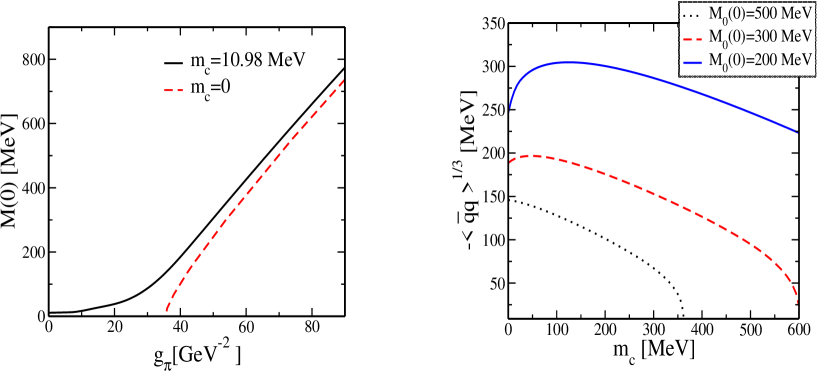
Figure 6.1: Quark condensate for various sets of parameters as a function of current quark mass (right). The dynamical quark mass at zero momentum as a function of coupling (left) for parameter set: $M_{0}(0)=300$ MeV, $\Lambda=860.58$ MeV $m_{c}=10.98$, the mass generation occur at critical coupling $g^{cr}_{\pi}=27.0$ [GeV^-2].

From the gap equation Eq. (6.4) one can show that dynamical symmetry breaking occurs for $1/g_{\pi}-1/g^{cr}_{\pi}<0$, where $1/g^{cr}_{\pi}=\frac{N_{c}N_{f}\Lambda^{2}}{12\pi^{2}}$, $N_{c}$ and $N_{f}$ are the number of colours and flavours, respectively. For $g_{\pi}>g_{\pi}^{cr}$ fermions become massive and the vacuum accommodates a non-vanishing condensate $\langle\bar{\psi}\psi\rangle$, and consequently there exists a massless Nambu-Goldstone boson, see Fig 6.1.

6.3 Meson channel

The quark-antiquark $T$-matrix in the pseudoscalar channel can be solved by using the Bethe-Salpeter equation in the random phase approximation (RPA), as shown in Fig. 6.2, see Ref. [135].

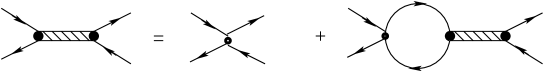
Figure 6.2: A graphical representation of the Bethe-Salpeter equation for the $\bar{q}q$ $T$-matrix in RPA approximation. The solid lines denote the dressed quark propagators Eq. (6.5) and shaded boxes denote meson propagators.

$$T(p_{1},p_{2},p_{3},p_{4}) = f(p_{1})f(p_{2})\big{[}i\gamma_{5}\tau_{i}\big{]}\frac{g_{\pi}i}{1+g_{\pi}J_{\pi}(q^{2})}\big{[}i\gamma_{5}\tau_{i}\big{]}f(p_{3})f(p_{4})$$ (6.8)

$$\times\delta(p_{1}+p_{2}-p_{3}-p_{4}),\$$

where

$$J_{\pi}(q^{2}) = i{\rm Tr}\int\frac{d^{4}k}{(2\pi)^{4}}f^{2}(k)\gamma_{5}\tau_{i}S(k)\gamma_{5}\tau_{i}S(q+k)f^{2}(q+k),$$ (6.9)

$$= 6i\int\frac{d^{4}k}{(2\pi)^{4}}{\rm tr}\;_{D}[\gamma_{5}S(k)\gamma_{5}S(k+q)]f^{2}(k)f^{2}(q+k),\$$

where $q$ denotes the total momentum of the $\bar{q}q$ pair. The pion mass $m_{\pi}$ corresponds to the pole of $T$-matrix. One immediately finds that $m_{\pi}=0$ if the current quark mass $m_{c}$ is zero, in accordance with Goldstone’s theorem. The residue of the $T$-matrix at this pole has the form

$$V^{\pi}(p_{1},p_{2})=ig_{\pi qq}[\leavevmode\hbox{\small 1\normalsize\kern-3.30002pt1}_{c}\otimes\tau^{a}\otimes\gamma_{5}]f(p_{1})f(p_{2}),$$ (6.10)

where $g_{\pi qq}$ is the pion-quark-antiquark coupling constant and is related to the corresponding loop integral $J_{\pi}$ by

$$g^{-2}_{\pi qq}=\left.\frac{dJ_{\pi}}{dq^{2}}\right|_{q^{2}=m^{2}_{\pi}}.$$ (6.11)

Notice that $Z=g^{2}_{\pi qq}$ can be regarded as a pion wavefunction renormalisation constant. For space-time dimension $D=4$, one can show $Z^{-1}\varpropto\Lambda^{2}$ (for the local NJL model we have $Z^{-1}\varpropto{\rm Ln}\Lambda$), therefore in the continuum limit $\Lambda\to\infty$ we have $Z=0$ which is precisely the compositeness condition [146]. In this extreme limit pions become pointlike. The cutoff for spacetime $D=4$ can be removed only at the expense of making the theory trivial in the continuum limit. It has been shown that for four-fermion theories the renormalisability, nontriviality and compositeness are intimately related [130, 147].

Figure 6.3: One-pion-to-vacuum matrix element in RPA, contributing to the weak pion decay. The lines are as defined in Fig. 6.2. The wavy line denotes a weak decay.

The pion decay constant $f_{\pi}$ is obtained from the coupling of the pion to the axial-vector current. Notice that due to the non-locality the axial-vector current is modified [135, 148] and consequently the one-pion-to-vacuum matrix element gets the additional contribution shown in Fig. 6.3. This new term is essential in order to maintain Gell-Mann-Oakes-Renner relation [135] and makes a significant contribution. The pion decay constant is given by

$$f_{\pi} = \frac{ig_{\pi\bar{q}q}}{m_{\pi}^{2}}\int\frac{d^{4}k}{(2\pi)^{4}}{\rm Tr}[q\kern-4.49997pt/\gamma_{5}\frac{\tau_{a}}{2}(S(p_{-}))\gamma_{5}\tau_{a}(S(p_{+}))]f(p_{-})f(p_{+})$$ (6.12)

$$+ \frac{ig_{\pi}}{2m^{2}_{\pi}}\int\frac{d^{4}k}{(2\pi)^{4}}{\rm Tr}[S(k)]\int\frac{d^{4}k}{(2\pi)^{4}}{\rm Tr}[V^{\pi}(p_{-},p_{+})S(p_{-})\gamma_{5}\tau_{a}S(p_{+})]$$

$$\times[f^{2}(k)\left(f^{2}(p_{+})+f^{2}(p_{-})\right)-f(p_{+})f(p_{-})f(k)\left(f(k+q)+f(k-q)\right)],\$$

where $V_{\pi}(p_{-},p_{+})$ is defined in Eq. (6.10), with notation $p_{\pm}=p\pm\frac{1}{2}q$.

Table 6.1: The parameters for the sets $A$ and $B$, fitted to $f_{\pi}=92.4$ MeV and $m_{\pi}=139.6$ MeV. Resulting values of the dynamical quark mass $M(0)$ are also shown.

Parameter	set A	set B
$M(0)$ (MeV)	297.9	351.6
$M_{0}(0)$ (MeV)	250	300
$m_{c}$ (MeV)	7.9	11.13
$\Lambda$ (MeV)	1046.8	847.8
$g_{\pi}(\text{GeV}^{-2})$	31.6	55.80

Table 6.2: The first two sets of poles of the quark propagator (in magnitude) in the Minkowski frame.

set A	set B
$\pm 391$ MeV	$\pm 408\pm 238i$ MeV
$\pm 675$ MeV	$\pm 1575\pm 307i$ MeV

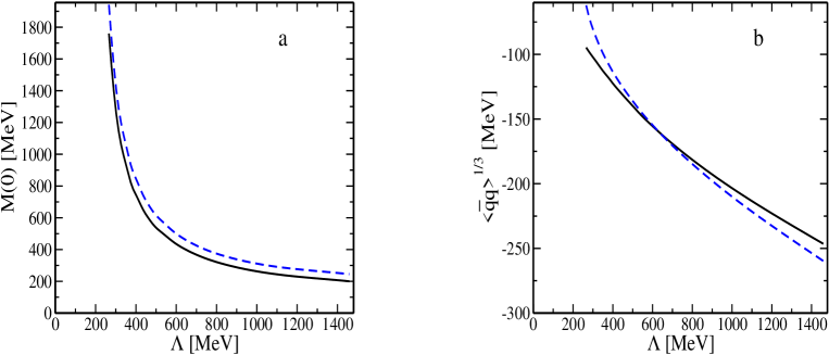
Figure 6.4: The dynamical quark mass at zero momentum (a) and quark condensate (b) with respect to the cutoff for fixed $f_{\pi}=93$ MeV and $m_{\pi}=140$ MeV. The solid line denotes the result when $m_{c}$ is not zero and the dashed line denotes the chiral limit $m_{c}=0$.

Our model contains five parameters: the current quark mass $m_{c}$, the cutoff ($\Lambda$), the coupling constants $g_{\pi}$ , $g_{s}$ and $g_{a}$. We first fix $g_{\pi}$ and the current quark mass $m_{c}$ for arbitrary values of $\Lambda$ by fitting $f_{\pi}$ and $m_{\pi}$ to their empirical values. In this way, we can consider the entire parameter space of the model. The corresponding solution of gap equation are shown in Fig. 6.4. In the left panel the constituent mass $M$ at zero momentum is shown as a function of the cutoff. It is obvious that for very small cutoff, there is no solution for the gap equation. On the right panel of Fig. 6.4, we show the corresponding values of the quark condensate. The quark condensate $\langle\bar{\psi}\psi\rangle=i{\rm Tr}S(0)$ is closely related to the gap equation Eq (6.4). In the latter there appears an extra form factor inside the loop integral. The quark condensate with non-zero current-quark mass is quadratically divergent and is regulated by a subtraction of its perturbative value. These values can fall within the limits extracted from QCD sum rules $190\text{MeV}\lesssim-\langle\bar{q}q\rangle^{1/3}\lesssim 260\text{MeV}$ at a renormalisation scale of $1$ GeV [149] and lattice calculation [150], having in mind that QCD condensate is a renormalised and scale-dependent quantity. In right-hand side of Fig. 6.1 we show the quark condensate with respect to current quark mass for various parameter sets, it is seen that for large coupling (or large $M(0)$), the magnitude of quark condensate decreases as the current quark mass increases. This feature is consistent with the behaviours of lattice and sum rule results.

We analyse two sets of parameters, see Table 6.1. The set $A$ is a non-confining parameter set, while set $B$ leads to quark confinement (i.e., it satisfies the condition Eq. (6.7). The quark condensate in the chiral limit is $-(207\text{ MeV})^{3}$ and $-(186\text{ MeV})^{3}$ for sets A and B, respectively. At non-zero current quark mass one obtains $-(215\text{MeV})^{3}$ and $-(191\text{MeV})^{3}$ for sets A and B respectively. The position of the quark poles are given in Table 6.2 for two sets of parameters. In Fig. 6.5 we show the position of the first pole of quark propagator with respect to various cutoff, which indicates that for large cutoff, we have only real poles and we have indeed complex poles for reasonable range of cutoff. The real part of the first pole of dressed quark propagator can be considered in much the same as the quark mass in the ordinary NJL model. Since we do not believe in on-shell quarks or quark resonances, this is also a measure for a limit on the validity of the theory. The real part of the first quark propagator pole $m^{\text{q}}_{R}$ is larger than the constituent quark mass at zero momentum $M(0)$, as can be seen in Table 6.1.

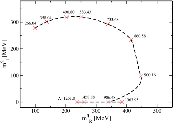
Figure 6.5: the position of the first poles of quark propagator in complex plane for various cutoff $\Lambda$ (MeV) for fixed $f_{\pi}=93$ MeV and $m_{\pi}=140$ MeV. For every point, there is a complex conjugate partner. The imaginary part and real part denote $m^{q}_{I}$ and $m^{q}_{R}$, respectively. Some values of cutoff are given on the plot.

As we will see the mass $m^{\text{q}}_{R}$ appears as an important parameter in diquark and nucleon solution rather than the constituent quark mass. The same feature has been seen in the studies of the soliton in this model, where $m^{\text{q}}_{R}$ determines the stability of the soliton [143]. In contrast to the local NJL model, here the dynamical quark mass Eq. (6.6) is momentum dependent and follows a trend similar to that estimated from lattice simulations [139]. Although this is less fundamental since one is free to choose the form factor, nevertheless the quark mass is a gauge dependent object and is not directly observable.

The parameters $g_{s}$ and $g_{a}$ are yet to be determined, we shall treat them as free parameters, which allows us to analyse baryon solutions in terms of a complete set of couplings. The coupling-constant dependence appears through the ratios $r_{s}=g_{s}/g_{\pi}$ and $r_{a}=g_{a}/g_{\pi}$.

6.4 Diquark channels

In the rainbow-ladder approximation the scalar $qq$ $T$-matrix can be calculated from a very similar diagram to that shown in Fig. 6.2 (the only change is that the anti-quark must be replaced by a quark with opposite momentum). It can be written as

$$T(p_{1},p_{2},p_{3},p_{4}) = f(p_{1})f(p_{2})\big{[}\gamma_{5}C\tau_{2}\beta^{A}\big{]}\tau(q)\big{[}C^{-1}\gamma_{5}\tau_{2}\beta^{A}\big{]}f(p_{3})f(p_{4})$$ (6.13)

$$\times\delta(p_{1}+p_{2}-p_{3}-p_{4}),\$$

with

$$\tau(q)=\frac{2g_{s}i}{1+g_{s}J_{s}(q^{2})},$$ (6.14)

where $q=p_{1}+p_{2}=p_{3}+p_{4}$ is the total momentum of the $qq$ pair, and

$$J_{s}(q^{2}) = i{\rm Tr}\int\frac{d^{4}k}{(2\pi)^{4}}f^{2}(-k)\big{[}\gamma_{5}C\tau_{2}\beta^{A}\big{]}S(-k)^{T}\big{[}C^{-1}\gamma_{5}\tau_{2}\beta^{A}\big{]}S(q+k)f^{2}(q+k),$$ (6.15)

$$= 6i\int\frac{d^{4}k}{(2\pi)^{4}}{\rm tr}\;_{D}[\gamma_{5}S(k)\gamma_{5}S(k+q)]f^{2}(k)f^{2}(q+k).$$

In the above equation the quark propagators $S(k)$ are the solution of the rainbow SDE Eq. (6.5). The denominator of Eq. (6.14) is the same as in the expression for the pion channel, Eq. (6.8), if $g_{s}=g_{\pi}$. One may thus conclude that at $r_{s}=1$ the diquark and pion are degenerate. This puts an upper limit to the choice of $r_{s}$, since diquarks should not condense in vacuum.

One can approximate $\tau(q)$ by an effective diquark exchange between the external quarks, and parametrise $\tau(q)$ around the pole as

$$\tau(q)\equiv 2ig^{2}_{dsqq}V^{s}(q)D(q),\hskip 56.9055ptD^{-1}(q)=q^{2}-M^{2}_{ds},$$ (6.16)

where $M_{ds}$ is the scalar diquark mass, defined as the position of the pole of $\tau(q)$. The strength of the on-shell coupling of scalar diquark to quarks, $g_{dsqq}$ is related to the polarisation operator $J_{s}$ by

$$g^{-2}_{dsqq}=\frac{dJ_{s}}{dq^{2}}|_{q^{2}=M^{2}_{ds}},$$ (6.17)

and $V^{s}(q)$ is the ratio between the exact $T$-matrix and on-shell approximation. It is obvious that we should have $V^{s}(q)|_{q^{2}=M^{2}_{ds}}=1$.

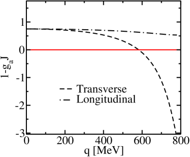
Figure 6.6: The denominator of the diquark $T$ matrix for the longitudinal and transverse axial vector channel. for parameter set A at $r_{a}=0.44$. Note that there is no longitudinal pole.

Here, there is no mixing between the axial-vector diquark channel with others, therefore in the same way one can write the axial-vector diquark $T$-matrix in a similar form

$$T(p_{1},p_{2},p_{3},p_{4}) = f(p_{1})f(p_{2})\big{[}\gamma_{\mu}C\tau_{i}\tau_{2}\beta^{A}\big{]}\tau^{\mu\nu}(q)\big{[}C^{-1}\gamma_{\nu}\tau_{2}\tau_{i}\beta^{A}\big{]}f(p_{3})f(p_{4})$$ (6.18)

$$\times\delta(p_{1}+p_{2}-p_{3}-p_{4}),\$$

with

$$\tau^{\mu\nu}(q)=2g_{a}i\Big{[}\frac{g^{\mu\nu}-q^{\mu}q^{\nu}/q^{2}}{1+g_{a}J^{T}_{a}(q^{2})}+\frac{q^{\mu}q^{\nu}/q^{2}}{1+g_{a}J^{L}_{a}(q^{2})}\Big{]}.$$ (6.19)

Here we prefer to decompose the axial polarisation tensor into longitudinal and transverse channels as well,

$$J^{\mu\nu}_{a}(q^{2}) = i{\rm Tr}\int\frac{d^{4}k}{(2\pi)^{4}}f^{2}(-k)\big{[}\gamma^{\mu}C\tau_{i}\tau_{2}\beta^{A}\big{]}S(-k)^{T}\big{[}C^{-1}\gamma^{\nu}\tau_{2}\tau_{i}\beta^{A}\big{]}S(q+k)f^{2}(q+k),$$ (6.20)

$$= 6i\int\frac{d^{4}k}{(2\pi)^{4}}{\rm tr}\;_{D}[\gamma^{\mu}S(k)\gamma^{\nu}S(k+q)]f^{2}(k)f^{2}(q+k)$$

$$= J^{T}_{a}(q^{2})(g^{\mu\nu}-q^{\mu}q^{\nu}/q^{2})+J^{L}_{a}(q^{2})q^{\mu}q^{\nu}/q^{2}.\$$

We find that the longitudinal channel does not produce a pole (see Fig. 6.6), and thus the bound axial-vector diquark solution corresponds to a pole of the transverse $T$-matrix. The transverse component of $\tau^{\mu\nu}(q)$ matrix is now approximated by $M_{da}$ as,

$$\tau^{\mu\nu}(q)\equiv 2ig^{2}_{daqq}V^{a}(q)D^{\mu\nu}(q),\hskip 56.9055ptD^{\mu\nu}(q)=\frac{g^{\mu\nu}-q^{\mu}q^{\nu}/q^{2}}{q^{2}-M^{2}_{da}},$$ (6.21)

where $V^{a}(q)$ includes the off-shell contribution to the $T$-matrix. The coupling constant $g_{daqq}$ is related to the residue at the pole of the $T$-matrix,

$$g^{-2}_{daqq}=\frac{dJ^{T}_{a}}{dq^{2}}|_{q^{2}=M^{2}_{da}}.$$ (6.22)

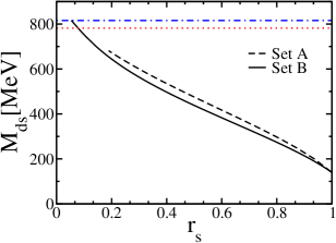
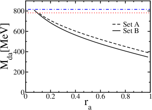
Figure 6.7: The scalar and axial-vector diquark mass as a function of $r_{s}$ and $r_{a}$, respectively, for both parameter sets. The dotted and broken-dotted lines lines denote the quark-quark pseudo-threshold for set A and B, respectively.

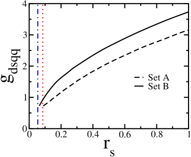
Figure 6.8: The scalar diquark-quark-quark coupling as a function of $r_{s}$. The dotted and broken-dotted lines indicate the quark-quark pseudo-threshold for set A and B, respectively.

6.4.1 Diquark Solution

The loop integrations in Eq. (6.15, 6.20) are evaluated in Euclidean space. For the current model, the usual analytic continuation of amplitudes from Euclidean to Minkowski space can not be used. This is due to the fact that quark propagators of the model contain many poles at complex energies leading to opening of a threshold for decay of a diquark (or meson) into other unphysical states. Any theory of this type need to be equipped with an alternative continuation prescription consistent with unitarity and macrocausality. Let us define a fictitious two-body threshold as twice $m^{\text{q}}_{R}$. For a confining parameter set, each quark propagator has a pair of complex-conjugate poles. Above the two-body pseudo-threshold $q^{2}<-4(m^{\text{q}}_{R})^{2}$, where $q$ is meson (diquark) momentum, the first pair of complex poles of the quark propagator has a chance to cross the real axis. According to the Cutkosky prescription [151], if one is to preserve the unitarity and the microcausality, the integration contour should be pinched at that point. In this way, one can ensure that there is no spurious $\bar{q}q$ (or $qq$) production threshold, for energies below the next pseudo-threshold, i.e. twice the real part of the second pole of the quark propagator. Note that it has been shown [152] that the removal of the $\bar{q}q$ pseudo-threshold is closely related to the existence of complex poles in the form of complex-conjugate pairs. Since there is no unique analytical continuation method available for such problems, any method must be regarded as a part of the model assumptions [135, 141, 152]. Here, we follow the method used in Ref. [135].

We use the parameter sets determined in the mesonic sector shown in table 6.1. Our numerical computation is valid below the first $qq$ pseudo-threshold. Note that the longitudinal polarisability $J^{L}_{a}(q)$ defined in Eq. (6.20) does not vanish here. However this term can probably be ignored since it does produce any poles in the $T$-matrix, and moreover there is no conserved current associated to this channel. We find that for a wide range of $r_{s}$ and $r_{a}$, for all parameter sets, a bound scalar and axial-vector diquark exist (the results for additional sets can be found in [32]). This is in contrast to the normal NJL model where a bound axial-vector diquark exists only for very strong interaction [120]. The diquark masses for various values of $r_{s}$ and $r_{a}$ are plotted in Fig. 6.7. As already pointed out, the scalar diquark mass is equal to the pion mass at $r_{s}=1$. It is obvious from Fig. 6.7 that for $r_{s}=r_{a}$ the axial-vector diquark is heavier than the scalar diquark, and consequently is rather loosely bound. For very small $r_{s}$ and $r_{a}$ one finds no bound state of either diquark. This kind of diquark confinement is due to the screening effect of the ultraviolet cutoff and can not be associated with confinement in QCD which originates from the infrared divergence of the gluon and ghost propagators. Having said that, it is possible that real diquark confinement may arise beyond the ladder approximation [154]. There, in order to preserve Goldstone’s theorem at every order, we must include additional terms in the interaction. Although these new terms should have minimal impact on the solutions for the colour-singlet meson channels, they can provide a repulsive contribution to the colour-antitriplet diquark channels which removes the asymptotic-diquark solutions from the spectrum. This would indicate that diquark confinement is an independent phenomenon and is not related to the particular realisation of quark confinement.

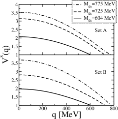
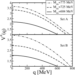
Figure 6.9: The ratio of the on-shell approximation compared to the exact diquark $T$-matrix for the various scalar and axial diquark masses.

One should note that the nucleon bound state in the diquark-quark picture does not require asymptotic-diquark states since the diquark state is merely an intermediate device which simplifies the three-body problem. Nevertheless, evidence for correlated diquark states in baryons is found in deep-inelastic lepton scatterings and in hyperon weak decays [157]. At the same time, diquarks appear as bound states in many phenomenological models. It is puzzling that diquarks are even seen in lattice calculations [155, 156]. In contrast to our perception of QCD colour confinement, the corresponding spectral functions for these supposedly confined objects in the colour anti-triplet channel are very similar to mesonic ones [156].

In Fig. 6.8, we show the scalar diquark-quark-quark coupling defined in Eq. (6.17) with respect to various scalar diquark couplings. A pronounced change in behaviour around the quark-quark pseudo-threshold is observed in the confining set $B$, and this seems to justify our emphasis on the pseudo-threshold defined by twice the real part of the quark pole.

Next we study the off-shell behaviour of the diquark $T$-matrix. In Fig. 6.9 we show the discrepancy between the exact $T$-matrix and the on-shell approximation $V^{s,a}(q)$. At the pole we have by definition that $V^{s,a}(q)|_{q^{2}=M^{2}_{s,a}}=1$. We see that elsewhere the off-shell contribution is very important due to the non-locality of our model. We find that the bigger the diquark mass is, the bigger the off-shell contribution. The off-shell behaviour of the scalar and the axial-vector channel for both parameter sets $A$ and $B$ are rather similar.

6.5 Three-body sector

In order to make three-body problem tractable, we discard any three-particle irreducible graphs (this is sometimes called the Faddeev approximation). The relativistic Faddeev equation can be then written as an effective two-body BS equation for a quark and a diquark due to the locality of the form factor in momentum space (see Eq. (6.3)) and accordingly the separability of the two-body interaction in momentum-space. We adopt the formulation developed by the Tübingen group [122, 123, 124] to solve the resulting BS equation. In the following we work in momentum space with Euclidean metric. The BS wave function for the octet baryons can be presented in terms of scalar and axialvector diquarks correlations,

$$\psi(p,P)u(P,s)=\left(\begin{array}[]{c}\psi^{5}(p,P)\\ \psi^{\mu}(p,P)\end{array}\right)u(P,s),$$ (6.23)

where $u(P,s)$ is a basis of positive-energy Dirac spinors of spin $s$ in the rest frame. The parameters $p=(1-\eta)p_{i}-\eta(p_{j}+p_{k})$ and $P=p_{i}+p_{j}+p_{k}$ are the relative and total momenta in the quark-diquark pair, respectively. The Mandelstam parameter $\eta$ describes how the total momentum of the nucleon $P$ is distributed between quark and diquark.

One may alternatively define the vertex function associated with $\psi(p,P)$ by amputating the external quark and diquark propagators (the legs) from the wave function;

$$\phi(p,P)=S^{-1}(p_{q})\tilde{D}^{-1}(p_{d})\left(\begin{array}[]{c}\psi^{5}(p,P)\\ \psi^{\nu}(p,P)\end{array}\right),$$ (6.24)

with

$$\tilde{D}^{-1}(p_{d})=\left(\begin{array}[]{cc}D^{-1}(p_{d})&0\\ 0&(D^{\mu\nu}(p_{d}))^{-1},\end{array}\right)$$ (6.25)

where $D(p),D^{\mu\nu}(p)$ and $S(p)$ are Euclidean versions of the diquark and quark propagators which are obtained by the standard transcription rules from the expressions in Minkowski space, Eqs. (6.16,6.21) and Eq. (6.5), respectively. The spectator quark momentum $p_{q}$ and the diquark momentum $p_{d}$ are given by

$$p_{q} = \eta P+p,$$ (6.26)

$$p_{d} = (1-\eta)P-p,\$$ (6.27)

with similar expressions for $k_{q,d}$, where we replace $p$ by $k$ on the right-hand side. In the ladder approximation, the coupled system of BS equations for octet baryon wave functions and their vertex functions takes the compact form,

$$\phi(p,P)=\int\frac{d^{4}k}{(2\pi)^{4}}K^{BS}(p,k;P)\psi(k,P),\\$$ (6.28)

where $K^{BS}(p,k;P)$ denotes the kernel of the nucleon BS equation representing the exchange quark within the diquark with the spectator quark (see Fig. 5.1), and in the colour singlet and isospin $\frac{1}{2}$ channel we find (see Ref. [120])

$$K^{BS}(p,k;P)=-3\left(\begin{array}[]{cc}\chi^{5}(p_{1},k_{d})S^{T}(q)\bar{\chi}^{5}(p_{2},p_{d})&-\sqrt{3}\chi^{\alpha}(p_{1},k_{d})S^{T}(q)\bar{\chi}^{5}(p_{2},p_{d})\\ -\sqrt{3}\chi^{5}(p_{1},k_{d})S^{T}(q)\bar{\chi}^{\mu}(p_{2},p_{d})&-\chi^{\alpha}(p_{1},k_{d})S^{T}(q)\bar{\chi}^{\mu}(p_{2},p_{d})\end{array}\right),$$ (6.29)

where $\chi$ and $\chi^{\mu}$ (and their adjoint $\bar{\chi}$ and $\bar{\chi}^{\mu}$) stand for the Dirac structures of the scalar and the axial-vector diquark-quark-quark vertices and can be read off immediately from Eqs. (6.13, 6.16) and Eqs. (6.18, 6.21), respectively. Therefore we have

$$\chi^{5}(p_{1},k_{d}) = g_{dsqq}(\gamma^{5}C)\sqrt{2V^{s}(k_{d})}f(p_{1}+(1-\sigma)k_{d})f(-p_{1}+\sigma k_{d}),$$

$$\chi^{\mu}(p_{1},k_{d}) = g_{daqq}(\gamma^{\mu}C)\sqrt{2V^{a}(k_{d})}f(p_{1}+(1-\sigma)k_{d})f(-p_{1}+\sigma k_{d}).\$$ (6.30)

We have used an improved on-shell approximation for the contribution of diquark $T$-matrix occurring in the Faddeev equations. Instead of the exact diquark $T$-matrices we use the on-shell approximation with a correction of their off-shell contribution through $V^{s,a}(p)$. What is neglected is then the contribution to the $T$-matrix beyond the pseudo-threshold. As we will see this approximation is sufficient to obtain a three-body bound state. In order to evaluate the structure of the diquark $T$-matrix completely, one normally employs the dispersion relation, however, this is not applicable here, due to non-analyticity of the diquark $T-$ matrix. Notice, as we already pointed out for the confining set B, we do not have $qq$ continuum, however, there exists many complex poles beyond the pseudo-threshold which might be ignored, provided that they lie well above the energies of interest.

The relative momentum of quarks in the diquark vertices $\chi$ and $\chi^{\mu}$ are defined as $p_{1}=p+k/2-(1-3\eta)P/2$ and $p_{2}=-k-p/2+(1-3\eta)P/2$, respectively. The momentum $k_{d}$ of the incoming diquark and the momentum $p_{d}$ of the outgoing diquark are defined in Eq. (6.27) (see Fig. 5.1). The momentum of the exchanged quark is fixed by momentum conservation at $q=-p-k+(1-2\eta)P$.

It is interesting to note the non-locality of the diquark-quark-quark vertices naturally provides a sufficient regularisation of the ultraviolet divergence in the diquark-quark loop. In the expressions for the momenta we have introduced two independent Mandelstam parameters $\eta,\sigma$, which can take any value in $[0,1]$. They parametrise different definitions of the relative momentum within the quark-diquark ($\eta$) or the quark-quark system ($\sigma$). Observables should not depend on these parameters if the formulation is Lorentz covariant. This means that for every BS solution $\psi(p,P;\eta_{1},\sigma_{1})$ there exists a equivalent family of solutions. This provides a stringent check on calculations, see the next section for details.

We now constrain the Faddeev amplitude to describe a state of positive energy, positive parity and spin $s=1/2$. The parity condition can be immediately reduced to a condition for the BS wave function:

$$\mathcal{P}\left(\begin{array}[]{c}\psi^{5}(p,P)\\ \psi^{\mu}(p,P)\end{array}\right)=\left(\begin{array}[]{c}\gamma^{4}\psi^{5}(\bar{p},\bar{P})\gamma^{4}\\ \gamma^{4}\Lambda^{\mu\nu}_{\mathcal{P}}\psi^{\nu}(\bar{p},\bar{P})\gamma^{4}\end{array}\right)=\left(\begin{array}[]{c}\psi^{5}(p,P)\\ -\psi^{\mu}(p,P)\end{array}\right),$$ (6.31)

where we define $\bar{p}=\Lambda_{\mathcal{P}}p$ and $\bar{P}=\Lambda_{\mathcal{P}}P$, with $\Lambda^{\mu\nu}_{\mathcal{P}}=\text{diag}(-1,-1,-1,1)$. In order to ensure the positive energy condition, we project the BS wave function with the positive-energy projector $\Lambda^{+}=(1+\hat{P\kern-6.49994pt/})$, where the hat denotes a unit four vector (in rest frame we have $\hat{P}=P/iM$). Now we expand the BS wave function $\psi(p,P)$ in Dirac space $\Gamma\in\{\textbf{1},\gamma_{5},\gamma^{\mu},\gamma_{5}\gamma^{\mu},\sigma^{\mu\nu}\}$. The above-mentioned conditions reduce the number of independent component from sixteen to eight, two for the scalar diquark channel, $S_{i},(i=1,2)$ and six for the axial-diquark channel, $A_{i},(i=1,...6)$. The most general form of the BS wave function is given by

$$\psi^{5}(p,P) = \left(S_{1}-i\hat{p\kern-4.49997pt/}_{T}S_{2}\right)\Lambda^{+},$$

$$\psi^{\mu}(p,P) = \Big{(}i\hat{P}^{\mu}\hat{p\kern-4.49997pt/}_{T}A_{1}+\hat{P}^{\mu}A_{2}-\hat{p}^{\mu}_{T}\hat{p\kern-4.49997pt/}_{T}A_{3}+i\hat{p}^{\mu}_{T}A_{4}+\left(\hat{p}^{\mu}_{T}\hat{p\kern-4.49997pt/}_{T}-\gamma^{\mu}_{T}\right)A_{5}$$ (6.32)

$$-(i\gamma^{\mu}_{T}\hat{p\kern-4.49997pt/}_{T}+i\hat{p}^{\mu}_{T})A_{6}\Big{)}\gamma_{5}\Lambda^{+}.\$$

Here we write $\gamma^{\mu}_{T}=\gamma^{\mu}-\hat{P\kern-6.49994pt/}\hat{P}^{\mu}$. The subscript $T$ denotes the component of a four-vector transverse to the nucleon momentum, $p_{T}=p-\hat{P}(p.\hat{P})$. In the same way, one can expand the vertex function $\phi$ in Dirac space, and since the same constraints apply to the vertex function, we obtain an expansion quite similar to Eq. (6.32), with new unknown coefficients $\mathbb{S}_{i}$ and $\mathbb{A}_{i}$ which are substituted the coefficients $S_{i}$ and $A_{i}$, respectively. The unknown scalar function $S_{i}(\mathbb{S}_{i})$ and $A_{i}(\mathbb{A}_{i})$ depend on the two scalars which can be built from the nucleon momentum $P$ and relative momentum $p$, $z=\hat{P}.\hat{p}=\cos\omega$ (the cosine of the four-dimensional azimuthal angle of $p^{\mu}$) and $p^{2}$.

In the nucleon rest frame, one can rewrite the Faddeev amplitude in terms of tri-spinors each possessing definite orbital angular momentum and spin [122]. It turns out that these tri-spinors can be written as linear combinations of the eight components defined in Eq. (6.32). Thus from knowledge of $S_{i}$ and $A_{i}$, a full partial wave decomposition can be immediately obtained [122]. Notice that although the diquarks are not pointlike objects here, they do not carry orbital angular momentum i. e. $L^{2}\chi^{5,\mu}(q)=0$. This is due to the fact that the off-shell contribution $V^{s,a}(q)$ is a function of scalar $q^{2}$. Moreover, the form factor in our model Lagrangian is also scalar, hence the total momentum dependent part of the diquark-quark-quark vertices are scalar functions and carry no orbital angular momentum. Therefore, the partial wave decomposition obtained in Ref. [122] for pointlike diquarks can be used here. Note that no such partial wave decomposition can be found if one uses the BS vertex function $\phi^{5,\mu}$ since the axial-vector diquark propagator mixes the space component of the vertex function and time component of the axial-vector diquark.

6.5.1 Numerical method for the coupled BS equations

For solving the BS equations we use the algorithm introduced by Oettel et al [125]. The efficiency of this algorithm has already been reported in several publications, see for example Refs. [122, 123, 124]. We will focus here only on the key ingredients of this method. The momentum dependence of quark mass in our model increases the complexity of the computation significantly.

As usual, we work in the rest frame of the nucleon $P=(0,iM_{N})$. In this frame we are free to chose the spatial part of the relative momentum $p$ parallel to the third axis. Thus the momenta $p$ and $k$ are given by

$$p^{\mu} = |p|(0,0,\sqrt{1-z^{2}},z),$$

$$k^{\mu} = |k|(\sin\theta^{\prime}\sin\phi^{\prime}\sqrt{1-z^{\prime 2}},\sin\theta^{\prime}\cos\phi^{\prime}\sqrt{1-z^{\prime 2}},\cos\theta\sqrt{1-z^{\prime 2}},z^{\prime}),\$$ (6.33)

where we write $z=\cos\omega$ and $z^{\prime}=\cos\omega^{\prime}$. The wave function Eq. (6.32) consists of $2\times 2$-blocks in Dirac space can be simplified to

$$\psi^{5}(p,P) = \left(\begin{array}[]{cc}S_{1}(p^{2},z)&0\\ \sigma_{3}\sqrt{1-z^{2}}S_{2}(p^{2},z)&0\end{array}\right),\hskip 34.14322pt\psi^{4}(p,P)=\left(\begin{array}[]{cc}\sigma_{3}\sqrt{1-z^{2}}A_{1}(p^{2},z)&0\\ A_{2}(p^{2},z)&0\end{array}\right),$$ (6.38)

$$\psi^{3}(p,P) = \left(\begin{array}[]{cc}i\sigma_{3}A_{3}(p^{2},z)&0\\ i\sqrt{1-z^{2}}A_{4}(p^{2},z)&0\end{array}\right),\hskip 42.67912pt\psi^{2}(p,P)=\left(\begin{array}[]{cc}i\sigma_{2}A_{5}(p^{2},z)&0\\ -\sigma_{1}\sqrt{1-z^{2}}A_{6}(p^{2},z)&0\end{array}\right),$$ (6.43)

$$\psi^{1}(p,P) = \left(\begin{array}[]{cc}i\sigma_{1}A_{5}(p^{2},z)&0\\ \sigma_{2}\sqrt{1-z^{2}}A_{6}(p^{2},z)&0\end{array}\right).\$$ (6.46)

The great advantage of this representation is that the scalar and the axial-vector components are decoupled. Therefore the BS equation decomposes into two sets of coupled equations, two for the scalar diquark channel and six for the axial diquark channel. We expand the vertex (wave) functions in terms of Chebyshev polynomials of the first kind, which are closely related to the expansion into hyperspherical harmonics. This decomposition turns out to be very efficient for such problems [122, 123, 124, 125]. Explicitly,

$$F^{\psi}_{i}(p^{2},z) = \sum^{n_{max}}_{n=0}i^{n}F^{\psi(n)}_{i}(p^{2})T_{n}(z),$$

$$F^{\phi}_{i}(p^{2},z) = \sum^{m_{max}}_{m=0}i^{n}F^{\phi(m)}_{i}(p^{2})T_{m}(z),\$$ (6.47)

where $T_{n}(z)$ is the Chebyshev polynomial of the first kind. We use a generic notation, the functions $F^{\psi}_{i}$( and $F^{\phi}_{i}$) substituting the function $S_{i},~{}A_{i}$ (and $\mathbb{S}_{i},~{}\mathbb{A}_{i}$),

$$S_{1,2}\to F^{\psi}_{1,2},\hskip 56.9055ptA_{1...6}\to F^{\psi}_{3...8},$$

$$\mathbb{S}_{1,2}\to F^{\phi}_{1,2},\hskip 56.9055pt\mathbb{A}_{1...6}\to F^{\phi}_{3...8}.$$ (6.48)

We truncate the Chebyshev expansions involved in $F^{\psi}_{i}$ and $F^{\phi}_{i}$ at different orders $n_{max}$ and $m_{max}$, respectively. We also expand the quark and diquark propagators into Chebyshev polynomials. In this way one can separate the $\hat{P}\cdot\hat{p}$ and $\hat{P}\cdot\hat{k}$ dependence in Eqs. (6.28–6.24). Using the orthogonality relation between the Chebyshev polynomials, one can reduce the four dimensional integral equation into a system of coupled one-dimensional equations. Therefore one can rewrite Eqs. (6.24, 6.28) in the matrix form

$$F^{\psi(n)}_{i}(p^{2}) = \sum_{j=1}^{8}\sum_{m=0}^{m_{max}}g_{ij}^{nm}(p^{2})F^{\phi(m)}_{j}(p^{2}),$$

$$F^{\phi(m)}_{i}(p^{2}) = \sum_{j=1}^{8}\sum_{n=0}^{n_{max}}\int^{\infty}_{0}d|k||k|^{3}H_{ij}^{mn}(k^{2},p^{2})F^{\psi(n)}_{j}(k^{2}).\$$ (6.49)

Here $g_{ij}^{nm}$ and $H_{ij}^{mn}$ are the matrix elements of the propagator and the quark exchange matrices, respectively. The indices $n,m$ give the Chebyshev moments and $i,j$ denote the individual channels. To solve Eq. (6.49), we first rewrite it in the form of linear eigenvalue problem. Schematically

$$\lambda(P^{2})\varphi=K(P^{2})\varphi,$$ (6.50)

with the constraint that $\lambda(P^{2})=1$ at $P^{2}=-M^{2}_{N}$. This can be used to determine the nucleon mass $M_{N}$ iteratively.

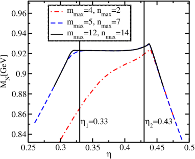
Figure 6.10: The dependence of the nucleon mass on the Mandelstam parameter $\eta$ for a few values of the cut-off on the expansion. Here we use set B, with $M_{ds}=725$ MeV and $M_{da}=630$ MeV. The variables $\eta_{1}$ and $\eta_{2}$ denote the position of the singularities.

As already pointed out the BS solution should be independent of the Mandelstam parameters $\eta,\sigma$. As can be seen in Fig. 6.10, there is indeed a large plateau for the $\eta$ dependence if we use a high cut-off on the Chebyshev moments. The limitations on the size of this area of stability can be understood by considering where the calculation contains singularities due to quark and diquark poles,

$$\eta \in \left[1-\frac{M_{ds}}{M_{N}},\frac{m^{\text{q}}_{R}}{M_{N}}\right],\hskip 56.9055pt\text{if}\hskip 28.45274ptM_{ds}<M_{da},$$

$$\eta \in \left[1-\frac{M_{da}}{M_{N}},\frac{m^{\text{q}}_{R}}{M_{N}}\right],\hskip 56.9055pt\text{if}\hskip 28.45274ptM_{da}<M_{ds}.$$ (6.51)

A similar plateau has been found in other applications [122, 123, 124]. [Other complex poles lies out side the minimal region given in Eq. (6.51).] The singularities in the quark-exchange propagator put another constraint on the acceptable range of $\eta$; $\eta>\frac{1}{2}(1-\frac{m^{\text{q}}_{R}}{M_{N}})$. No such constraint exists for $\sigma$, which relates to the relative momentum between two quarks. To simplify the algebra we take $\sigma=1/2$.

In what follows we use a momentum mesh of $60\times 60$ for $p,k$, mapped in a non-linear way to a finite interval. In the non-singular regime of Mandelstam parameter $\eta$ Eq. (6.51), the Faddeev solution is almost independent of the upper limit on the Chebyshev expansion, and for $m_{max}=10,n_{max}=12$, see the Fig. 6.10, this seems to be satisfied. This limit is some higher than the reported values for simple models [122, 123, 124, 125].

6.5.2 Nucleon Solution

In order to understand the role of the axial diquark in nucleon solution, we first consider the choice $r_{a}=0$. For this case we find that the non-confining set A can not generate a three-body bound state in this model without the inclusion of the off-shell contribution. For the confining set B one also has to enhance the diquark-quark-quark coupling $g_{dsqq}$ by a factor of about $1.73$ over the value defined in Eq. (6.17) (as we will show, this extra factor is not necessary when the axial-vector is included). The situation is even more severe in the on-shell treatment of the local NJL model, since one needs to include the full $qq$ continuum contribution in order to find a three-body bound state when the axial-vector diquark channel is not taken into account [118].

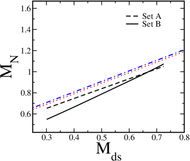
Figure 6.11: The nucleon mass without inclusion of the axial diquark channel. The dotted lines indicate the diquark-quark threshold. All values are given in GeV.

As can be seen from Fig. 6.7 a decrease in $r_{s}$ leads to a larger diquark mass, and an increase in the off-shell contribution to the $qq$ $T$-matrix (see Fig. 6.9). It is this off-shell correction is need for a bound nucleon.

The nucleon result is shown in Fig. 6.11. We also show a fictitious diquark-quark threshold defined as $M_{ds}+m^{\text{q}}_{R}$. The nucleon mass can be seen to depend roughly linearly on the scalar diquark mass. A similar behaviour is also seen in the local NJL model [119]. Increasing the diquark mass (or decreasing $r_{s}$) increases the nucleon mass, i.e. the scalar diquark channel is attractive. In order to obtain a nucleon mass of $940$ MeV, we need diquark mases of $608$ MeV and $623$ MeV for set A and B, respectively. The corresponding nucleon binding energy measured from the diquark-quark threshold are $56$ MeV and $91$ MeV for set A and B, respectively, compared to the binding of the diquarks (relative to the $qq$ pseudo threshold) of about $174$ and $193$ MeV for set A and B, respectively. Such diquark clustering within the nucleon is also observed in the local NJL model [119], and is qualitatively in agreement with a instanton model [158] and lattice simulations [159]. The nucleon solutions for sets A and B behave rather differently with respect to the diquark-quark threshold, see Fig. 6.12. This indicates that for non-confining set A, the nucleon solution is rather sensitive to the diquark-quark threshold and tends not avoid it. However, for confining set, since there is no well-defined threshold, this tendency is absent and as we approach to the diquark-quark threshold, the nucleon binding energy decreases and can approach to zero.

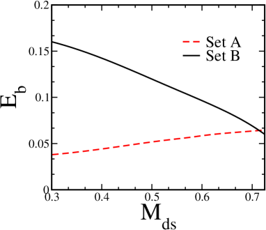
Figure 6.12: The nucleon binding energy measured from the diquark-quark threshold with respect to scalar diquark mass. Only scalar diquarks are included in the calculation The smooth behaviour of solid line indicates the absence of threshold effects for the confining case.

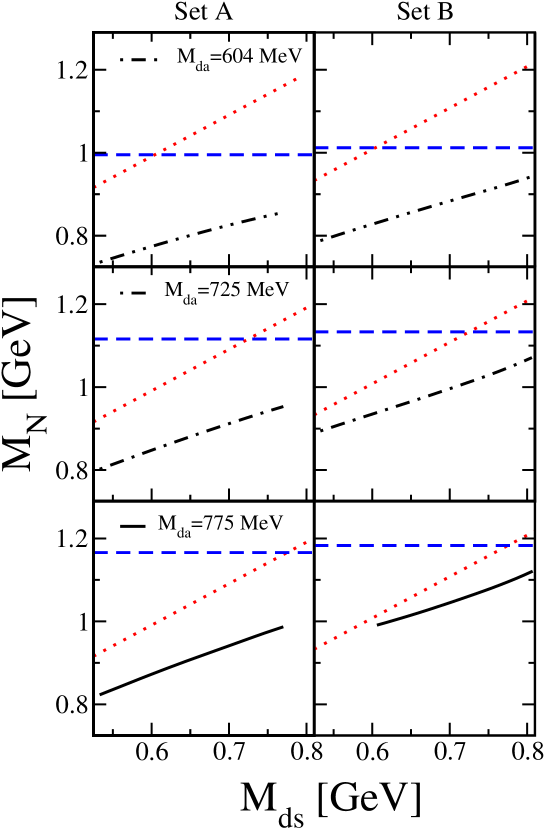
Figure 6.13: The nucleon mass as a function of the scalar diquark mass. The dotted lines are the scalar diquark-quark threshold, the broken lines are the axial vector diquark-quark threshold. All values are given in GeV.

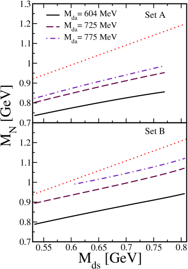
Figure 6.14: The nucleon mass as a function of the scalar diquark mass for various axial vector diquark masses for both parameter sets. The scalar diquark-quark threshold are shown by the doted lines.

Next we investigate the effect of the axial-vector diquark channel on nucleon solution. We find that the axial-vector diquark channel contributes considerably to the nucleon mass and takes away the need for the artificial enhancement of the coupling strength for set B. In Figs. 6.13, 6.14 we show the nucleon mass as a function of the scalar and axial-vector diquark mass. Similar to the scalar diquark channel, we define the axial-vector diquark-quark threshold as $M_{da}+m^{\text{q}}_{R}$. We see that as one increase the axial-vector diquark (and scalar diquark) masses, the $qq$ interaction is weakened and consequently the nucleon mass is increases. Therefore the contribution of the axial-vector channel to the nucleon mass is also attractive.

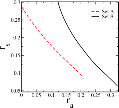
Figure 6.15: Range of parameters $(r_{s},r_{a})$ where we find a nucleon mass of $940$ MeV.

In Fig. 6.15 we plot the parameter space of the interaction Lagrangian with variable $r_{s}$ and $r_{a}$ which leads to the nucleon mass $M_{N}=0.940$ GeV. The trend of this plot for the non-confining set A is very similar to the one obtained in the local NJL model [120] (although we use a different parameter set) and roughly depends linearly on the ratios $r_{s}$ and $r_{a}$,

$$M_{N}[0.940\text{GeV}]=-r_{s}-0.94r_{a}+1.2.$$ (6.52)

Therefore, any interaction Lagrangian with $r_{s}$ and $r_{a}$ which satisfies the relation $r_{s}+0.94r_{a}=0.30$ gives a nucleon mass at about the experimental value. This relation shows how interaction is shared between scalar and axial-vector channels. If the scalar diquark interaction $r_{s}$ is less than $0.14$, we need the axial-vector interaction to be stronger than the scalar diquark channel $r_{a}>r_{s}$ in order to get the experimental value of nucleon mass. For set B, as we approach to $r_{a}=0$, the curve bends upward, reflecting the fact that we have no bound state with only scalar diquark channel. In Fig. 6.15 we see for the confining set B that the interaction is again shared between the scalar and the axial-vector diquark and for small $r_{s}<0.19$ one needs a dominant axial-vector diquark channel $r_{a}>r_{s}$. It is obvious that the axial-vector diquark channel is much more important in the confining than the non-confining phase of model.

Table 6.3: Diquark masses and coupling of diquarks to quarks obtained for $M_{N}=0.940$. All masses are given in MeV. $E_{ds}(E_{da})$ denote the binding energy of diquarks in the nucleon, $E^{ds}_{N}(E^{da}_{N})$ denote the binding energy of the nucleon measured from scalar (axial) diquark mass.

	Set A			Set B
	Set A1	Set A2	Set A3	Set B1	Set B2	Set B3
$M_{ds}$	775	748	698	802	705	609
$g_{dsqq}$	0.74	0.83	1.04	0.73	1.31	1.79
$r_{s}$	0.09	0.12	0.17	0.06	0.14	0.24
$E_{ds}$	7	34	84	14	111	207
$E^{ds}_{N}$	226	199	149	270	173	77
$M_{da}$	705	725	775	604	660	725
$g_{daqq}$	1.08	0.98	0.79	1.99	1.67	1.28
$r_{a}$	0.20	0.17	0.11	0.32	0.23	0.15
$E_{da}$	77	57	7	212	156	91
$E^{da}_{N}$	156	176	226	72	123	193
$p_{\bot}^{\text{RMS}}$	194.88	181.51	163.70	283.99	232.86	209.95

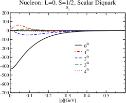
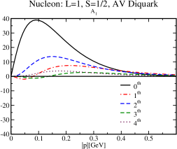
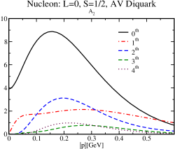
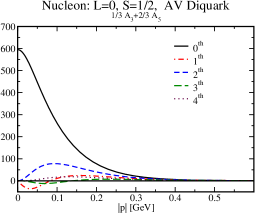
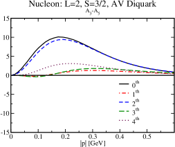
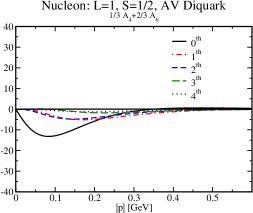
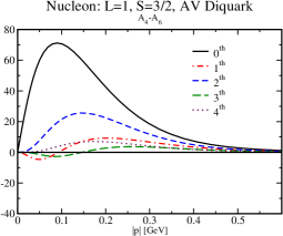
Figure 6.16: Different Chebyshev moments (labeled by $n^{th}$) of scalar and axialvector (AV) diquark amplitudes of the nucleon BS wave function given by Set A1.

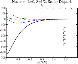
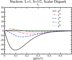
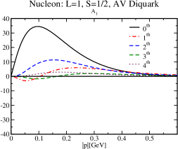
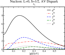
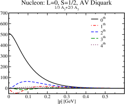
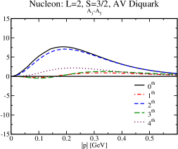
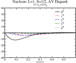
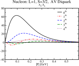
Figure 6.17: Different Chebyshev moments (labeled by $n^{th}$) of scalar and axialvector diquark amplitudes of the nucleon wave function given by Set A2.

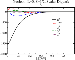
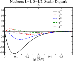
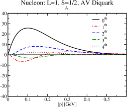
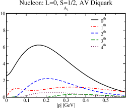
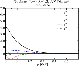
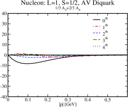
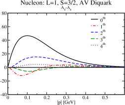
Figure 6.18: Different Chebyshev moments (labeled by $n^{th}$) of scalar and axialvector diquark amplitudes of the nucleon wave function given by Set A3.

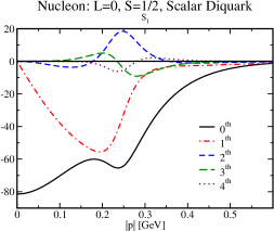
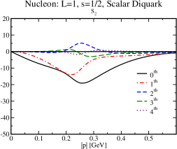
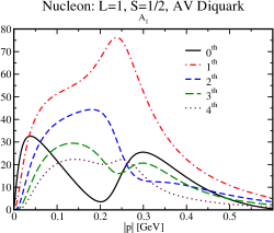
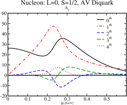
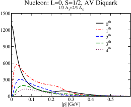
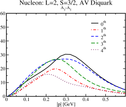
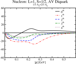
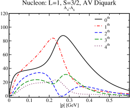
Figure 6.19: Different Chebyshev moments (labeled by $n^{th}$) of scalar and axialvector (AV) diquark amplitudes of the nucleon BS wave function given by Set B1.

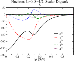
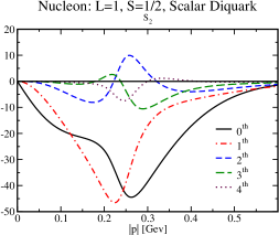
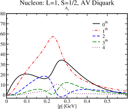
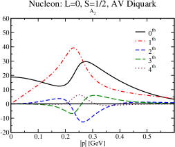
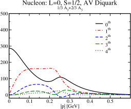
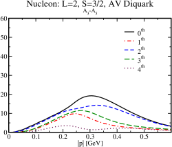
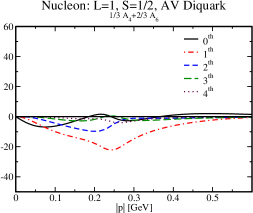
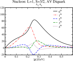
Figure 6.20: Different Chebyshev moments (labeled by $n^{th}$) of scalar and axialvector diquark amplitudes of the nucleon wave function given by Set B2.

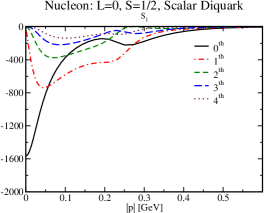
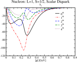
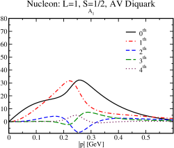
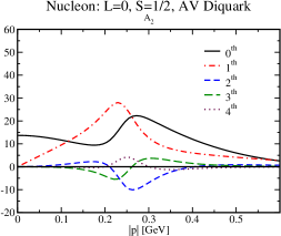
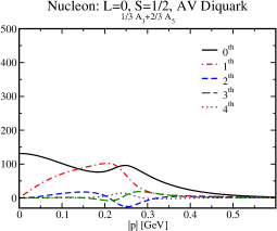
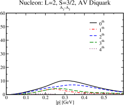
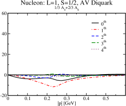
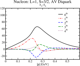
Figure 6.21: Different Chebyshev moments (labeled by $n^{th}$) of scalar and axialvector diquark amplitudes of the nucleon wave function given by Set B3.

In order to study the implications of the quark confinement for the description of the nucleon, we compare in Table 6.3 three representative cases for both the non-confining and confining parameter sets, which all give nucleon mass about $940$ MeV. The first three columns contain results for set $A$, and the last three columns for the confining set $B$.

Given the definition of diquark-quark thresholds, in the presence of both scalar and axial-vector diquark channels, the diquarks in the nucleon can be found much more loosely bound, although one obtains a very strongly bound nucleon solution near its experimental value, see table 6.3. Next we study the nucleon BS wave function for the various sets given in Table 6.3. The nucleon wave and vertex function are not physical observables, but rather they suggest how observables in this model will behave. In Figs. 6.16-21 we show the leading Chebyshev moments of the scalar functions of the nucleon BS wave function for various sets (A1-3 and B1-3) which describes the strengths of the quark-diquark partial waves with $S$ as a total quark-diquark spin and $L$ as a total orbital angular momentum. They are normalised to $F_{1}^{\phi(0)}(p_{1})=1$, where $p_{1}$ is the first point of the momentum mesh. It is seen that the contribution of higher moments are considerably small, indicating a rapid convergence of the wave function amplitudes in terms of Chebyshev polynomials. In the confining case Figs. 6.19-21 there is a clear interference which is not present in the non-confining Figs. 6.16-19. Therefore in the confining case, all wave function amplitudes are somehow shifted to higher relative four-momenta between diquark and quark. In order to understand the role of this interference we obtain a mass density for the various channels. This density is defined as

$$\rho(p_{\bot},P)=\int dp_{4}\psi^{{\dagger}}(p_{\bot},p_{4},P)\tilde{D}^{-1}(p_{d})\psi(p_{\bot},p_{4},P)$$ (6.53)

where $p_{\bot}$ stands for space component of relative momentum $p$ and $\tilde{D}^{-1}(p_{d})$ defined in Eq. (6.25). This definition corresponds to a diagram occurring for the calculation of the isoscalar quark condensate in the impulse approximation [121]. In the above definition of the density function, we have integrated over the time component of the relative momentum. In this way the density function becomes very similar to its counterpart in Minkowski space. Although the above definition of density is not unique, it does provide a useful measure of the spatial extent of the wave function (we have examined the possibility of taking matrix elements of other operators between the BS wave function, since this does not lead to any significant effect, the results are not presented here). The results are plotted in Figs. 6.22 and 6.23.

It is noticeable that in various sets, the $s$-wave is the dominant contribution to the ground state. The relative importance of the scalar and the axial diquark amplitude in the nucleon changes with the strength of the diquark-quark couplings $g_{dsqq}(g_{daqq})$ and accordingly with $r_{s}(r_{a})$. We see that in the confining sets, the nucleon density extends to higher relative momentum between the diquark and the quark. This indicates a more compact nucleon in the confining case. In order to find a qualitative estimation of the confinement effect in our model, we calculate $p_{{\bot}}^{\text{RMS}}=(\langle p^{2}_{\bot}\rangle-\langle p_{\bot}\rangle^{2})^{1/2}$, the results can be found in table 6.3. This can be related to the mean-square radius of the nucleon, if we assume minimal uncertainty. We see in the both confining and non-confining cases a decrease in $p_{{\bot}}^{\text{RMS}}$ with weakening axial-vector diquark interaction (and consequently increasing the scalar diquark interaction strength). If we compare $p_{{\bot}}^{\text{RMS}}$ for the two sets $A2,B2$, which have very similar interaction parameters $r_{s}(r_{a})$, an increase about $25\%$ is found. This effect can not only be associated with the non-locality of our interaction, since that is present in both confining and non-confining cases.

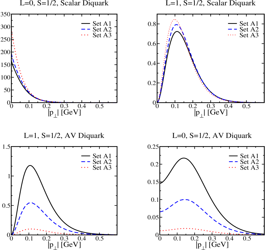
Figure 6.22: Shows the nucleon density ($M=0.940$ GeV, Set $A$) with respect to relative momentum between diquark and quark for different set of $A1,A2$ and $A3$.

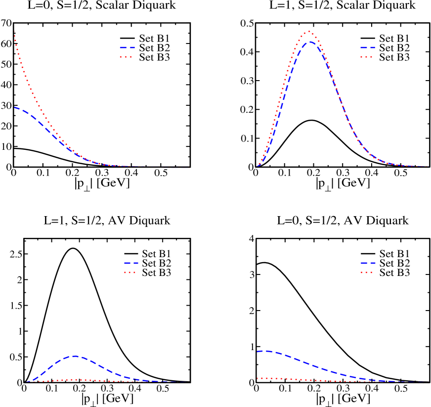
Figure 6.23: Shows the nucleon density ($M=0.940$ GeV, Set $B$) with respect to relative momentum between diquark and quark for different set of $B1,B2$ and $B3$.

6.6 Summary and Outlook

In this chapter we investigated the two- and three-quark problems in a non-local NJL model. We have truncated the diquark sector to the bound scalar and the axial-vector channels. We have solved the relativistic Faddeev equation for this model and have studied the behaviour of the nucleon solutions with respect to various scalar and the axial-vector interactions. We have also investigated a possible implication of the quark confinement of our model in the diquark and the baryon sector.

Although the model is quark confining, it is not diquark confining (at least in the rainbow-ladder approximation). A bound diquark can be found in both scalar and the axial-vector channel for a wide range of couplings. We have found that the off-shell contribution to the diquark $T$-matrix is crucial for the calculation of the structure of the nucleon: without its inclusion the attraction in the diquark channels is too weak to form a three-body bound state. We have also found that both the scalar and the axial-vector contribute attractively to the nucleon mass. The role of axial-vector channel is much more important in the confining phase of model. The nucleon in this model is strongly bound although the diquarks within nucleon are loosely bound. The confining aspects of the model are more obvious in three-body, rather than the two-body sector. By investigating the nucleon wave function we showed that quark confinement leads to a more compact nucleon. The size of nucleon is reduced by about $25\%$ in confining phase.

For both confining and non-confining phases, an increase in the scalar diquark channel interaction $r_{s}$ leads to a lower nucleon mass, see Figs. 6.13 and 6.14, but the mass of the $\Delta$ remains unchanged since it does not contain scalar diquarks. In the standard NJL model where the axial-vector diquark does not contribute significantly to the nucleon binding [127, 161, 162], the difference between the $\Delta$ and nucleon mass is directly related to the scalar diquark interaction. In the current model where the axial-vector diquark makes a larger contribution to the nucleon mass, therefore a detailed calculation for the delta states is needed to understand the mechanism behind the $\Delta$-$N$ mass difference. In the standard NJL model this leads to a contradiction, since for an axial-vector interaction which gives a reasonable description of nucleon properties, both the axial-vector diquark and more importantly the $\Delta$ are unbound [162]. The crucial role of the axial-vector diquark correlation in the non-local NJL model, especially in the confining phase of the model, indicate that this model might do better.

In order to understand the implications of this model in baryonic sector fully one should investigate properties of the nucleon such as the axial vector coupling constant, the magnetic moment, etc. On the other hand, the role of quark confinement in this model can be better clarified by investigating quark and nuclear matter in this model. One of the long standing problem in four-Fermi chiral quark models is the fact that quark/nuclear matter does not saturate [163], mainly due to the strongly attractive quark interactions responsible for the spontaneous chiral symmetry breaking. Recently, Bentz and Thomas [164] have shown that a sufficient strong repulsive contribution can arise if confinement effects are incorporated, albeit in the cost of introducing a new parameter into model. It was shown that such repulsive contribution can lead to saturation of nuclear matter equation of state. It is indeed of interest to investigate the stability of nuclear matter within this quark confining model. Such problems can be studied based on the Faddeev approach, see e. g., Ref. [131].

Bibliography

- [1] F. Coester, Nucl. Phys. 7, 42 (1957); F. Coester and H. Kümmel, Nucl. Phys. 17, 477 (1960).
- [2] For example: R. F. Bishop and H. G. Kümmel, Phys. Today 40, No. 3, 52, (1987).
- [3] J. Arponen, Ann, Phys. (N.Y) 151, 311 (1983); J. S. Arponen, R. F. Bishop and E. Pajanne, Phys. Rev. A36, 2519 (1987); A36, 2539 (1987); J. Arponen, R. F. Bishop, E. Pajanne and N. I. Robinson, Phys. Rev. A37, 1065 (1988); N. I. Robinson and R. F. Bishop, Phys. Rev A40, 4256 (1989); J. S. Arponen and R. F. Bishop, Phys. Rev. Lett. 64, 111 (1990); J. S. Arponen and R. F. Bishop, Ann. Phys (N.Y) 227, 334 (1993).
- [4] J. S. Arponen and R. F. Bishop, Ann. Phys (N.Y) 207, 171 (1991); 227, 275 (1993).
- [5] R. F. Bishop in: Microscopic Quantum many body theories and their applications, edited by J. Navarro and A. Polls. Lecture notes in Physics 510, 1 (1997); R. F. Bishop, Theor. Chim. Acta. 80, 95 (1991).
- [6] J. Goldstone, Proc. Roy. Soc. (London) A239, 267 (1957).
- [7] M. Gell-mann and F. Low , Phys. Rev 84, 350 (1951).
- [8] U. Kaulfuss, Phys. Rev D32, 1421 (1985).
- [9] R. Hagg, K. Dan, Vidensk. selsk. Mat. Fys. Medd. 29, 12 (1955).
-
[10]
R. Offerman, H. Kümmel and W. Ey, Nucl. Phys A273, 349 (1976);
W. Ey, Nucl. Phys A296, 189 (1978). - [11] W. Pauli, Phys. Rev 58, 716 (1940).
- [12] V. A. Kostelecky and R. Lehnert, Phys. Rev D63, 065008, (2001).
- [13] H. Blum and R. Brockmann, Phys. Rev C59, 2546 (1999).
- [14] J. Thouless, The Quantum Mechanics of Many Body System, New York (1961).
- [15] H. Kümmel, Phys. Rev C27, 765 (1983).
- [16] B. Brandow, Rev. Mod. Phys 39, 771 (1967).
- [17] A. S. Wightman, Phys. Rev. 101, 860 (1956).
- [18] R. Hagg, Local Quantum physics, fields, particles, Algebras, Springer-Verlag, (1992). N. N. Bogolubov, A. A. Logunov, I. T. Todorov, Introduction to axiomatic quantum field theory, Benjamin (1975).
- [19] T. J. Hollowood, V. V. Khoze, W. Lee and M. P. Mattis, Nucl. Phys. B570, 241 (2000).
- [20] R. Alkofer and L. von Smekal, Phys. Rept. 353, 281 (2001).
- [21] F. Strocchi, Phys. Rev. D17, 2010 (1978).
- [22] I. Ojima, Nucl. Phys. B143, 340 (1978); Z. Phys. C5,227 (1980).
- [23] M. Nakahara, Geometry, Topology and Physics, IOP (1990).
- [24] L. von Smekal and R. Alkofer, Phys. Rev. Lett. 79, 3591 (1997); K. Buttner, M. R. Pennington, Phys. Rev. D52, 5220 (1995); UKQCD collaboration (Derek B. Leinweber et al.), Phys. Rev. D58, 031501 (1998).
- [25] K. G. Wilson and J. B. Kogut, Phys. Rep. 12C, 75 (1974); K. G. Wilson, Rev. Mod. Phys. 47, 773 (1975); C. Bagnuls and C. Bervillier, Phys. Rept. 348, 91 (2001).
- [26] S. Weinberg, Phys. Rev. 166, 1568 (1968); J. Gasser and H. Leutwyler, Ann. Phys. (N.Y.) 158, 142 (1984).
- [27] R. J. Perry, A. Harindranath and K. G. Wilson, Phys. Rev. Lett. 65, 24, 2959 (1990).
- [28] For example: G. Hasberg and H. Kümmel, Phys. Rev. C33, 1367 (1986); H. G. Kümmel, Phys. Rev. D50, 6556 (1993).
- [29] S. D. Glazek and K. G. Wilson, Phys. Rev. D48, 5863 (1993); S. D. Glazek and K. G. Wilson, Phys. Rev. D49, 4218 (1994).
- [30] F. Wegner, Ann. Physik (Berlin) 3, 77 (1994).
- [31] For example: A. P. Szczepaniak and E. S. Swanson, Phys. Rev. D55, 1578 (1997); E. L. Gubankova and F. Wegner, Phys. Rev. D58, 025012 (1998); T. Maslowski and M. Wieckowski, Phys. Rev. D57, 4976 (1998); T. S. Walhout, Phys. Rev. D59, 065009 (1999); D. G. Robertson, E. S. Swanson, A. P. Szczepaniak and C. R. Ji, S. R. Cotanch, Phys. Rev. D59, 074019 (1999); G. Alexanian and E. F. Moreno, Phys. Lett. B450, 149 (1999); D. Chakrabarti and A. Harindranath, Phys. Rev. D65, 045001 (2002).
- [32] A. H. Rezaeian and N. R. Walet, JHEP 0312, 040 (2003).
- [33] A. H. Rezaeian and N. R. Walet, Phys. Lett. B570,129 (2003); A. H. Rezaeian and N. R. Walet, hep-th/0310205.
- [34] For example: F. J. Dyson, Phys. Rev. 102, 1217 (1956); 1230 (1956); D. Janssen, F. D nau, S. Frauendorf and R. V. Jolos, Nucl. Phys. A172, 145 (1971).
- [35] J. Arponen, Phys. Rev. A55, 2686 (1997).
- [36] K. Suzuki and S. Y. Lee, Prog. Theor. Phys. 64, 209 (1980).
- [37] K. Suzuki and R. Okamoto, Prog. Theor. Phys. 75, 1388 (1986); 76, 127 (1986); 92, 1045 (1994).
- [38] K. Suzuki, Prog. Theor. Phys. 87, 937 (1992); H. Kümmel, Phys. Rev. C27, 765 (1983); K. Suzuki, R. Okamoto and H. Kumaga, Nucl. Phys. A580, 213 (1994) and references therein.
- [39] K. Suzuki, Prog. Theor. Phys. 68, 246 (1982); T. T. S. Kuo, P. J. Ellis, J. Hao, Z. Li, K. Suzuki, R. Okamoto and H. Kumagai, Nucl. Phys. A560, 621 (1993).
- [40] K. Suzuki, R. Okamoto, P. J. Ellis, J. Hao, Z. Li, T. T. S. Kuo, Phys. Lett. B308, 1 (1993).
- [41] C. S. Hsue, H. Kümmel and P. Ueberholz, Phys. Rev. D32, 1435 (1985).
- [42] I. Tamm, J. Phys. USSR 9, 499(1945); S. M. Dancoff, Phys. Rev. 78, 382 (1950).
- [43] K. G. Wilson, Phys. Rev. 140, B445 (1965); K. G. Wilson, Phys. Rev. D2, 1438 (1970).
- [44] C. Bloch, Nucl. Phys. 6, 329 (1958).
- [45] J. P. Vary and A. Harindranath, In Nuclear and Particle Physics on the light cone, edited by M. B. Johnson and L. S. Kisslinger, World Scientific, Singapore, (1989), and references therein.
- [46] Weinberg, Phys. Rev. 150, 1313 (1966).
- [47] For example: R. J. Perry and A. Harindranath, Phys. Rev. D43, 4051 (1991); K. G. Wilson, T. S. Walhout, A. Harindranath, W. M. Zhang, R. J. Perry and S. D. Glazek, Phys. Rev. D49, 6720 (1994); M. Brisudova and R. Perry, Phys. Rev. D54, 1831 (1996).
- [48] U. Kaulfuss, Phys. Rev. D32, 6, 1421 (1985).
- [49] For example: R. J. Perry, Ann. Phys.(N.Y) 232, 166 (1994).
- [50] C. Itzykson and J. Zuber, Quantum Field Theory, McGraw-Hill, New York (1980).
- [51] R. J. Perry and K. G. Wilson, Nucl. Phys. B403, 587 (1993); R. Oehme, K. Sibold and W. Zimmermann, Phys. Lett. B147, 115 (1984).
- [52] R. J. Perry, Phys. Rept. 348, 33 (2001).
- [53] M. Gell-Mann, F. E. Low, Phys. Rev. 95, 1300 (1954).
- [54] P. Navratil, H. B. Geyer and T. T. S. Kuo, Phys. Lett. B315, 1 (1993).
- [55] C. Bloch and J. Horowitz, Nucl. Phys. 8, 91 (1958).
- [56] H. Feshbach, Ann. Phys. (N.Y) 19, 287 (1962).
- [57] P. J. Ellis and E. Osnes, Rev. Mod. Phys. 49, 777 (1977).
- [58] K. Suzuki and R. Okamoto, Prog. Theor. Phys. 71, 1221 (1984).
- [59] H. Osborn, Nucl. Phys. B294, 595 (1987); G. M. Shore, Nucl .Phys. B362, 85 (1991); J. Polonyi and K. Sailer, Phys. Rev. D63 105006 (2001).
- [60] M. Lassig, Nucl. Phys. B334, 652 (1990); B. P. Dolan, Int. J. Mod. Phys. A10, 2439 (1995); A10, 2703 (1995); A12, 2413 (1997); B. P. Dolan and A. Lewis, Phys. Lett. B460, 302 (1999);
- [61] M. Henneaux and C. Teitelboim, Quantization of Gauge Systems, Princeton University press, Princeton, NJ, (1992).
- [62] T. R. Morris, Int. J. Mod. Phys. A9, 2411 (1994).
- [63] M. T. Vaughn, R. Aaron and R. D. Amado, Phys. Rev. 124, 15, 1258 (1961).
- [64] C. M. Bender and C. Nash, Phys. Rev. D10, 1753 (1974).
- [65] J. R. Morris, R. Acharya and B. P. Nigan, Phys. Rev. D21, 2429 (1980).
- [66] M. G. Fuda, Phys. Rev. C26, 204 (1982).
- [67] C. Callan and D. Gross, Phys. Rev. D8, 4383 (1973).
- [68] K. A. Brueckner, Phys. Rev. 100, 36 (1955); H. A. Bethe, B. H. Brandow and A. G. Petschek, Phys. Rev. 129, 225 (1963). R. Machleidt, Int. J. Mod. Phys. B15, 1535 (2001).
- [69] T. Mizutani and D. S. Koltun, Ann. Phys. 109, 1 (1977).
- [70] M. G. Fuda, Phys. Rev C31, 1365 (1985).
- [71] S. Okubo, Prog. Theor. Phys. 12, 603 (1954).
- [72] D. Schütte, J. D. Providencia, Nucl. Phys. A338, 463 (1980).
- [73] S. S. Schweber, An introduction to relativistic quantum field theory, Peterson and Co., Evanstone (1961); J. Denschlag, L. Tiator and D. Drechsel, Eur. Phys. J. A3, 171 (1998).
- [74] G. Wentzel, Helv. Phys. Acta 15, 111 (1942).
- [75] J. D. Providencia, Nucl. Phys 54, 572 (1963); J. D. Providencia and C. M. Shakin, Phys. Rev. C4, 1560 (1971).
- [76] J. D. Providencia, C. M. Shakin, Phys. Rev. C4, 1560 (1971).
- [77] M. Stingl and A. T. Stelbovics, J. Phys. G4, 1371 (1978); M. Sawicki and D. Schütte, Z. Naturforsch. 36A, 1261 (1981).
- [78] D. Schütte, Nucl. Phys. A221, 450 (1974); K. Kottoff, Nucl. Phys. A221, 450 (1974).
- [79] M. E. Peskin and D. V. Schroeder,An Introduction to quantum field theory, Addison-Wesley, Reading, USA (1995).
- [80] Particle Data Group, Phys. Rev. D54, 1 (1996).
- [81] H. Pagels, Phys. Rep. 16, 219 (1976).
- [82] G. ’t Hooft, Phys. Rep. 142, 357 (1986).
- [83] R. T. Crewther, Phys. Rev. lett. 28, 1421 (1972); M. S. Chanowitz and J. ellis, Phys. Lett. B40, 397 (1972).
- [84] L. D. Fadeev and V. N. Popov, Phys. Lett. B25, 29 (1967).
- [85] J. C. Collins, Renormalization, Cambridge Univ. Press, UK (1984).
- [86] D. E. Groom, et. at., Eur. Phys. J. C15, 1 (2000).
- [87] D. J. Gross and F. Wilczek, Phys. Rev. Lett. 30, 1343 (1973).
- [88] G. Plunien, B. Muller and W. Greiner, Phys. Rept. 134, 87 (1986).
- [89] For example: A. H. Rezaeian and A. A. Saharian, Class. Quant. Grav. 19, 3625 (2002); M. R. Setare, A. H. Rezaeian, Mod. Phys. Lett. A15, 2159 (2000).
- [90] C. D. Roberts and A. G. Williams, Prog. Part. Nucl. Phys. 33, 477 (1994); C. D. Roberts and S. M. Schmidt, Prog. Part. Nucl. Phys. 45, S1 (2000).
- [91] P. Maris, A. Raya, C. D. Roberts and S.M. Schmidt, Eur. Phys. J. A18, 231 (2003); C. D. Roberts, nucl-th/0007054.
- [92] K. D. Lane, Phys. Rev. D10, 2605 (1974); H. D. Politzer, Nucl. Phys. B117, 397 (1976).
- [93] P. O. Bowman, U. M. Heller, A. G. Williams, Phys. Rev. D66, 014505 (2002).
- [94] Edited by N. Isgur, Quark confinement and the Hadron spectrum III, USA (1998).
- [95] R. Alkofer, P. G. Reinhard and H. Reinhardt, Chiral quark dynamics,Berlin, Springer (1995); D. Ebert, H. Reinhardt and M. K. Volkov, Prog. Part. Nucl. Phys. 33,1 (1994).
- [96] R. T. Cahill, C. D. Roberts, Phys. Rev. D32, 2419 (1985).
- [97] M. Schaden, H. Reinhardt, P. A. Amundsen and M. J. Lavelle, Nucl. Phys. B339, 595 (1990).
- [98] For reviews see: U. Vogl and W. Weise, Prog. Part. Nucl. Phys. 27, 195 (1991); S. P. Klevansky, Rev. Mod. Phys. 64, 649 (1992); J. Bijnens, Phys. Rept. 265, 369 (1996).
- [99] D. Diakonov, V. Yu. Petrov, Sov. Phys. JETP 62, 204 (1985); Nucl. Phys. B245, 259 (1984); D. Diakonov, V. Yu. Petrov, P. V. Pobylitsa, Nucl. Phys. B306, 809 (1988); I. V. Anikin, A. E. Dorokhov, L. Tomio, Phys. Part. Nucl. 31, 509 (2000).
- [100] S. Weinberg, Physica, 96A, 327 (1979).
- [101] J. Gasser and H. Leutwyler, Ann. Phys. 158, 142 (1984).
- [102] For example: M. Buballa, hep-ph/0402234 and references therein.
- [103] E. Witten, Nucl. Phys. 160, 57 (1979).
- [104] L. J. Reinders, H. Rubinstein and S. Yazaki, Phys. Rept. 127, 1 (1985).
- [105] T. H. R. Skyrme, Proc. Roy. Soc. A260, 127 (1961).
- [106] G. ’t Hooft, Nucl. Phys. B72, 461 (1974).
- [107] G. Holzwarth and B. Schwesinger,Rept. Prog. Phys. 49, 825 (1986).
- [108] H. Weigel, Int. J. Mod. Phys. A11, 2419 (1996); R. Alkofer, H. Reinhardt and H. Weigel, Phys. Rept. 265, 139 (1996).
- [109] E. Witten, Nucl. Phys. B223, 422 (1983).
- [110] J. Wess and B. Zumino, Phys. Lett. B37, 95 (1971).
- [111] T. D. Cohen, hep-ph/0312191.
- [112] P. Hasenfratz and J. Kuti, Phys. Rept. 40, 75 (1978).
- [113] R. K. Bhaduri, Models of the Nucleon: From Quarks to Soliton, Addison Wesley, Redwood City, USA (1988).
- [114] M. Rho, A. S. Goldhaber, G. E. Brown, Phys. Rev. Lett. 51, 747 (1983).
- [115] J. Goldestone and R. L. Jaffe, Phys. Rev. Lett. 51, 1518 (1983).
- [116] G. E. Brown, A. D. Jackson and M. Rho and V. Vento, Phys. Lett. B140, 285 (1984).
- [117] M. Rho, Phys. Rept. 240, 1 (1994).
- [118] A. Buck, R. Alkofer and H. Reinhardt, Phys. Lett. B286, 29 (1992).
- [119] S. Huang and J. Tjon, Phys. Rev. C49, 1702 (1994).
- [120] W. Bentz, H. Mineo, H. Asami, K. Yazaki, Nucl. Phys. A587,617 (1995).
- [121] C. Hanhart and S. Krewald, Phys. Lett. B344, 55 (1995); H. Asami, N. Ishii, W. Bentz and K. Yazaki, Phys. Rev. C51, 3388 (1995).
- [122] M. Oettel, G. Hellstern, R. Alkofer, H. Reinhardt, Phys. Rev. C58, 2459, (1998).
- [123] G. Hellstern, R. Alkofer, M. Oettel and H. Reinhardt, Nucl. Phys. A627, 679 (1997); M. Oettel, R. Alkofer, L. von Smekal, Eur. Phys. J. A8, 553 (2000).
- [124] S. Ahlig, R. Alkofer, C.S. Fischer, M. Oettel, H. Reinhardt, H. Weigel, Phys. Rev. D64, 014004 (2001).
- [125] M. Oettel, L. V. Smekal, R. Alkofer, Comput. Phys. Commun. 144, 63 (2002).
- [126] M. Oertel, M. Buballa and J. Wambach, Phys. Lett. B477, 77 (2000); Nucl. Phys. A676, 247 (2000); G. Ripka, Nucl. Phys. A683 463, 486 (2001).
- [127] G. Hellstern and C. Weiss, Phys. Lett. B351, 64 (1995).
- [128] K. Langfeld, C. Kettner and H. Reinhardt, Nucl. Phys. A608, 331 (1996).
- [129] J. Meyer, K. Schwenzer, H.-J. Pirner and A. Deandrea, Phys. Lett. B526, 79 (2002).
- [130] K. Shizuya, Phys. Rev. D21, 2327 (1980).
- [131] S. Pepin, M. C. Birse, J. A. McGovern and N. R. Walet, Phys. Rev. C61, 055209 (2000).
- [132] L. V. Smekal, P. A. Amundsen and R. Alkofer, Nucl. Phys. A529, 633 (1991).
- [133] J. M. Cornwall, Phys. Rev. D22, 1452 (1980); M. Stingl, Phys. Rev. D34, 3863 (1986); D36, 651 (1987); V. Sh. Gogoghia and B. A. Magradze, Phys. lett. B217, 162 (1989).
- [134] K. Langfeld and M. Rho, Nucl. Phys. A596, 451 (1996); D. Ebert, T. Feldmann and H. Reinhardt, Phys. Lett. B388, 154 (1996).
- [135] R. D. Bowler and M. C. Birse, Nucl. Phys. A582, 655 (1995); R. S. Plant and M. C. Birse, Nucl. Phys. A628, 607 (1998).
- [136] D. Atkinson and D. W. E. Blatt, Nucl. Phys. B151, 342 (1979).
- [137] P. Maris and H. A. Holties, Int. J. Mod. Phys. A7, 5369 (1992); S. J. Stainsby and R. T. Cahill, Int. J. Mod. Phys. A7, 7541 (1992); P. Maris, Phys. Rev. D50, 4189 (1994).
- [138] P. Maris, Phys. Rev. D52, 6087 (1995).
- [139] J. Skullerud, D. B. Leinweber and A. G. Williams, Phys. Rev. D64, 074508 (2001).
- [140] R. S. Plant and M. C. Birse, Nucl. Phys.A703, 717 (2002).
- [141] A. Scarpettini, D. G. Dumm and N. N. Scoccola, Phys. Rev. D69, 114018 (2004).
- [142] I. General, D. G. Dumm and N. N. Scoccola, Phys .Lett. B506, 267 (2001); D. G. Dumm and N. N. Scoccola, Phys. Rev. D65, 074021 (2002).
- [143] W. Broniowski, B. Golli and G. Ripka, Nucl. Phys. A703, 667 (2002), B. Golli, W. Broniowski and G. Ripka, Phys. Lett. B437, 24 (1998).
- [144] A. H. Rezaeian, N. R. Walet and M. C. Birse, Phys. Rev. C70, 065203 (2004).
- [145] T. Schäfer and E. V. Schuryak, Rev. Mod. Phys. 70, 323 (1998); D. Diakonov, Prog. Part. Nucl. Phys. 36, 1 (1996).
- [146] S. Weinberg, Phys. Rev. 130, 776 (1963).
- [147] S. Hands, A. Kocic and J. B. Kogut, Phys. Lett. B273, 111 (1991); Annals Phys. 224, 29 (1993).
- [148] J. W. Bos, J. H. Koch and H. W. L. Naus, Phys. Rev. C44, 485 (1991); W. Broniowski, hep-ph/9909438.
- [149] H. G. Dosch and S. Narison, Phys. Lett.B417,173 (1998).
- [150] L. Giusti, F. Rapuano, M. Talevi and A. Vladikas, Nucl. Phys. B538, 249 (1999).
- [151] R. E. Cutkosky, P. V. Landshoff, D. I. Olive and J. C. Polkinghorne, Nucl. Phys. B12, 281 (1969).
- [152] M. S. Bhagwat, M. A. pichowsky and P. C. Tandy, Phys. Rev. D67, 054019 (2003).
- [153] A. H. Rezaeian, N. R. Walet and M. C. Birse, hep-ph/0310013.
- [154] A. Bender, C. D. Roberts and L. V. Smekal, Phys. Lett B380, 7 (1997); G. Hellstern, R. Alkofer and H. Reinhardt, Nucl. phys. A625, 697 (1997).
- [155] M. Hess, F. Karsch, E. Laermann and I. Wetzorke, Phys. Rev. D58, 111502 (1998).
- [156] I. Wetzorke and F. Karsch, hep-lat/0008008.
- [157] M. Anselmino, E. Predazzi, S. Ekelin, S. Fredriksson and D. B. Lichtenberg, Rev. Mod. Phys. 65, 1199 (1993) and references therein.
- [158] T. Schafer, E. V. Shuryak, J. J. M. Verbaarschot, Nucl. Phys. B412, 143 (1994).
- [159] M. C. Chu, J.M. Grandy, S. Huang and J. W. Negele, Phys. Rev. D49, 6039 (1994).
- [160] M. B. Hecht, M. Oettel, C. D. Roberts, S. M. Schmidt, P. C. Tandy and A. W. Thomas, Phys. Rev. C65, 055204 (2002); N. Ishii, Phys. Lett. B431, 1 (1998).
- [161] C. Weiss, A. Buck, R. Alkofer and H. Reinhardt, Phys. Lett. B312, 6 (1993); V. Keiner, Z. Phys. A354, 87 (1996).
- [162] H. Mineo, W. Bentz, N. Ishii and K. Yazaki, Nucl. Phys. A703, 785 (2002).
- [163] for example: M. Buballa, Nucl. Phys. A611, 393 (1996).
- [164] W. Bentz, A. W. Thomas, Nucl. Phys.A696, 138 (2001).