Factorization and polarization in two charmed-meson B decays

Abstract

We provide a comprehensive test of factorization in the heavy-heavy $B$ decays motivated by the recent experimental data from BELLE and BABAR collaborations. The penguin effects are not negligible in the $B$ decays with two pseudoscalar mesons. The direct CP asymmetries are found to be a few percent. We give estimates on the weak annihilation contributions by analogy to the observed annihilation-dominated processes. The $N_{c}$ insensitivity of branching ratios indicates that the soft final state interactions are not dominant. We also study the polarizations in $B\to D^{*}D_{(s)}^{*}$ decays. The power law shows that the transverse perpendicular polarization fraction is small. The effects of the heavy quark symmetry breaking caused by the perturbative QCD and power corrections on the transverse polarization are also investigated.

I Introduction

The study of $B$ meson weak decays is of high interest in heavy flavor physics and CP violation. In particular, much attention has been paid to the two-body charmless hadronic $B$ decays, but there are relatively less discussions on the decays with charmful mesons, such as the modes with two charmed-meson in which the final states are both heavy. However, the two charmed-meson decays can provide some valuable and unique information which is different from the light meson productions. For example, CP asymmetries in the decays of $B\to D^{(*)+}D^{(*)-}$ play important roles in testing the consistency of the standard model (SM) as well as exploring new physics SX . Moreover, these decays are ideal modes to check the factorization hypothesis as the phenomenon of color transparency for the light energetic hadron is not applicable. Since the decay branching ratios (BRs), CP asymmetries (CPAs) and polarizations of $B\to D^{(*)}D^{(*)}(D^{(*)}D^{(*)}_{s})$ have been partially observed in experiments PDG04 ; BELLE_DD ; BABAR_DD , it is timely to examine these heavy-heavy $B$ decays in more detail.

At the quark level, one concludes that the two charmed-meson decays are dominated by tree contributions since the corresponding inclusive modes are $b\to qc\bar{c}$ with $q=s$ and $d$. It is known that the factorization has been tested to be successful in the usual color-allowed processes. However, the mechanism of factorization in heavy-heavy decays is not the same as the case of the light hadron productions. The color transparency argument Bjorken for light energetic hadrons is no longer valid to the modes with heavy-heavy final states. The reason can be given as follows. Due to the intrinsic soft dynamics in the charmed-meson, non-vanishing soft gluon contributions are involved in the strong interactions between an emission heavy meson with the remained $BD^{(*)}$ system. Since the corresponding divergences may not be absorbed in the definition of the hadronic form factor or hadron wave function, the decoupling of soft divergences is broken. This means that the mechanism of factorization has to be beyond the perturbative frameworks, such as QCD factorization BBNS and soft-collinear effective theory SCET . The large $N_{c}$ limit is another mechanism to justify factorization BGR , corresponding to the effective color number $N_{c}=\infty$ in the naive factorization approach BSW . The understanding of factorization in heavy-heavy decays requires some quantitative knowledge of non-perturbative physics which is not under control in theory. In this paper, we will assume the factorization hypothesis and apply the generalized factorization approach (GFA) GFA1 ; GFA2 to calculate the hadronic matrix elements.

It is known that annihilation contributions and nonfactorizable effects with final state interactions (FSIs) play important role during the light meson production in $B$ meson decays. For instance, to get large strong phases for CP asymmetries (CPAs) in $B\to K\pi$ and $B\to\pi\pi$ decays, these effects are included inevitably KLS_PRD63 ; CCS_PRD71 . Moreover, they are also crucial to explain the anomaly of the polarizations in $B\to\phi K^{*}$ decays, measured by BABAR babar_pol and BELLE belle_pol recently. By the naive analysis in flavor diagrams, one can easily see that the decay modes of $B\to D^{(*)0}\bar{D}^{(*)0}$ and $D^{(*)0}_{s}\bar{D}^{(*)0}_{s}$ are annihilation-dominated processes. Therefore, measurements of these decays will clearly tell us the importance of annihilation contributions in the production of two charmed-meson modes.

For the color-allowed decays, since the short-distant (SD) nonfactorizable parts are associated with the Wilson coefficient (WC) of $C_{1}/N_{c}$, where $C_{1}$ is induced by the gluon-loop and it is much smaller than $C_{2}\sim 1$, we can see that the effects arising from the SD non-spectator contributions should be small LM . Nevertheless, long-distant (LD) nonfactorizable contributions governed by rescattering effects or FSIs may not be negligible. Inspired by the anomaly of the large transverse perpendicular polarization, denoted by $R_{\perp}$, in $B\to\phi K^{*}$ decays, if there exist significant LD effects, we believe that large values of $R_{\perp}$ may appear in $B\to D^{*}D^{*}$ and $B\to D^{*}D^{*}_{s}$ too. As we will discuss, the power-law in the two-vector charmed-meson decay leads to a small $R_{\perp}$. The recent measurement of the polarization fraction by the BELLE collaboration gives $R_{\perp}=0.19\pm 0.08\pm 0.01$ BELLE_DD in which the central value is about a factor of three comparing with the model-independent prediction within the factorization approach and heavy quark symmetry. Clearly, to get the implication from the data, we need a detailed analysis in two charmful final states of $B$ decays.

To estimate the relevant hadronic effects for two-body decays in the $B$ system, we use the GFA, in which the leading effects are factorized parts, while the nonfactorized effects are lumped and characterized by the effective number of colors, denoted by $N^{\rm eff}_{c}$. Note that the scale and scheme dependences in effective WCs $C^{\rm eff}_{i}$ are insensitive. In the framework of the GFA, since the formulas for decay amplitudes are associated with the transition form factors, we consider them based on heavy quark effective theory (HQET) NeubertHQET . We will also study their $\alpha_{s}$ NeubertQCD and power corrections which break heavy quark symmetry (HQS) NR . In our analysis, we will try to find out the relationship between the HQS and its breaking effects for $R_{\perp}$. In addition, we will reexamine the influence of penguin effects, neglected in the literature LR . We will show that sizable CPAs in $\bar{B}^{0}\to D^{+}D^{-}$ and $B^{-}\to D^{0}D^{-}$ decays may rely on FSIs.

This paper is organized as follows. In Sec. II, we give the effective Hamiltonian for the heavy-heavy B decays. The definition of heavy-to-heavy form factors are also introduced. In Sec. III, we show the general formulas for B to two charmful states in the framework of the GFA. The effects of the heavy quark symmetry breaking on the transverse perpendicular polarization are investigated. In Sec. IV, we provide the numerical predictions on the BRs, direct CPAs and the polarization fractions. Conclusions are given in Sec. V. We collect all factorized amplitudes for $B\to PP,~{}PV(VP)$ and $VV$ decays in Appendixes.

II Effective interactions and parametrization of form factors

The relevant effective Hamiltonian for the $B$ meson decaying to two charmful meson states is given by BBL ,

$$H_{\rm eff}(\Delta B=1) = \frac{G_{F}}{\sqrt{2}}\left\{V_{ub}V_{uq}^{*}[C_{1}(\mu)O^{u}_{1}+C_{2}(\mu)O^{u}_{2}]+V_{cb}V_{cq}^{*}[C_{1}(\mu)O^{c}_{1}+C_{2}(\mu)O^{c}_{2}]\right.$$ (1)

$$\left.-V_{tb}V_{tq}^{*}\sum_{k=3}^{10}C_{k}(\mu)O_{k}\right\}+H.c.\;,$$

where $q=s$ and $d$, $V_{ij}$ denote the Cabibbo-Kobayashi-Masikawa (CKM) matrix elements, $C_{i}(\mu)$ are the Wilson coefficients (WCs) and $O_{i}$ are the four-fermion operators, given by

$$O^{u}_{1}=(\bar{q}_{i}u_{j})_{V-A}(\bar{u}_{j}b_{i})_{V-A},\;\;\;\;\;\;\;\;O^{u}_{2}=(\bar{q}_{i}u_{i})_{V-A}(\bar{u}_{j}b_{j})_{V-A},$$

$$O^{c}_{1}=(\bar{q}_{i}c_{j})_{V-A}(\bar{c}_{j}b_{i})_{V-A},\;\;\;\;\;\;\;\;\;O^{c}_{2}=(\bar{q}_{i}c_{i})_{V-A}(\bar{c}_{j}b_{j})_{V-A},$$

$$O_{3(5)}=(\bar{q}_{i}b_{i})_{V-A}\sum_{q^{\prime}}(\bar{q}^{\prime}_{j}q^{\prime}_{j})_{V\mp A},\;\;\;\;\;\;\;\;O_{4(6)}=(\bar{q}_{i}b_{j})_{V-A}\sum_{q^{\prime}}(\bar{q}^{\prime}_{j}q^{\prime}_{i})_{V\mp A},$$

$$O_{7(9)}=\frac{3}{2}(\bar{q}_{i}b_{i})_{V-A}\sum_{q^{\prime}}e_{q^{\prime}}(\bar{q}^{\prime}_{j}q^{\prime}_{j})_{V\pm A},\;\;O_{8(10)}=\frac{3}{2}(\bar{q}_{i}b_{j})_{V-A}\sum_{q^{\prime}}e_{q^{\prime}}(\bar{q}^{\prime}_{j}q^{\prime}_{i})_{V\pm A}.$$ (2)

with $i$ and $j$ being the color indices, $O_{3-6}$ ($O_{7-10}$) the QCD (electroweak) penguin operators and $(\bar{q}_{1}q_{2})_{V\pm A}=\bar{q}_{1}\gamma_{\mu}(1\pm\gamma_{5})q_{2}$. In order to cancel the renormalization scale and scheme dependence in the WCs of $C_{i}(\mu)$, the effective WCs are introduced by

$$C(\mu)\langle O(\mu)\rangle\equiv C^{\rm eff}\langle O\rangle_{\rm tree}.$$ (3)

Since the matrix element $\langle O\rangle_{\rm tree}$ is given at tree level, the effective WCs are renormalization scale and scheme independent. To be more useful, we can define the effective WCs as

$$a^{\rm eff}_{1} = C_{2}^{\rm eff}+\frac{C_{1}^{\rm eff}}{(N_{c}^{\rm eff})_{1}},~{}~{}~{}~{}~{}~{}a^{\rm eff}_{2}=C_{1}^{\rm eff}+\frac{C_{2}^{\rm eff}}{(N_{c}^{\rm eff})_{2}},$$

$$a^{\rm eff(q)}_{3,4} = C_{3,4}^{\rm eff}+\frac{C_{4,3}^{\rm eff}}{(N_{c}^{\rm eff})_{4,3}}+\frac{3}{2}e_{q}\left(C_{9,10}^{\rm eff}+\frac{C_{10,9}^{\rm eff}}{(N_{c}^{\rm eff})_{10,9}}\right),$$

$$a^{\rm eff(q)}_{5,6} = C_{5,6}^{\rm eff}+\frac{C_{6,5}^{\rm eff}}{(N_{c}^{\rm eff})_{6,5}}+\frac{3}{2}e_{q}\left(C_{7,8}+\frac{C_{8,7}^{\rm eff}}{(N_{c}^{\rm eff})_{8,7}}\right),$$ (4)

where

$$\frac{1}{(N_{c}^{\rm eff})_{i}}\equiv\frac{1}{N_{c}}+\chi_{i}.$$ (5)

with $\chi_{i}$ being the non-factorizable terms. In the GFA, $1/(N_{c}^{\rm eff})_{i}$ are assumed to be universal and real in the absence of FSIs. In the naive factorization, all effective WCs $C_{i}^{\rm eff}$ are reduced to the corresponding WCs of $C_{i}$ in the effective Hamiltonian and the non-factoziable terms are neglected, i.e., $\chi_{i}=0$.

Under the factorization hypothesis, the tree level hadronic matrix element $\langle O\rangle_{\rm tree}$ is factorized into a product of two matrix elements of single currents, which are represented by the decay constant and form factors. The $B\rightarrow H\left(H=D,\ D^{*}\right)$ transition form factors are crucial ingredients in the GFA for the heavy-heavy decays. To obtain the transition elements of $B\rightarrow H$ with various weak vertices, we first parameterize them in terms of the relevant form factors under the conventional forms as follows:

$$\langle D|V_{\mu}|\bar{B}\rangle = F_{1}(q^{2})\Big{\{}P_{\mu}-\frac{P\cdot q}{q^{2}}q_{\mu}\Big{\}}+\frac{P\cdot q}{q^{2}}F_{0}(q^{2})\,q_{\mu},$$ (6)

$$\langle D^{*}(\epsilon)|V_{\mu}|\bar{B}\rangle = \frac{V(q^{2})}{m_{B}+m_{D^{*}}}\varepsilon_{\mu\alpha\beta\rho}\epsilon^{*\alpha}P^{\beta}q^{\rho},$$

$$\langle D^{*}(\epsilon)|A_{\mu}|\bar{B}\rangle = i\left[2m_{D^{*}}A_{0}(q^{2})\frac{\epsilon^{*}\cdot q}{q^{2}}q_{\mu}+(m_{B}+m_{D^{*}})A_{1}(q^{2})\Big{(}\epsilon_{\mu}^{*}-\frac{\epsilon^{*}\cdot q}{q^{2}}q_{\mu}\Big{)}\right.$$ (7)

$$\left.-A_{2}(q^{2})\frac{\epsilon^{*}\cdot q}{m_{B}+m_{D^{*}}}\Big{(}P_{\mu}-\frac{P\cdot q}{q^{2}}q_{\mu}\Big{)}\right],$$

where $V_{\mu}=\bar{q}\gamma_{\mu}b$, $A_{\mu}=\bar{q}\gamma_{\mu}\gamma_{5}b$, $m_{B,D,D^{*}}$ are the meson masses, $\epsilon_{\mu}$ denotes the polarization vector of the $D^{*}$ meson, $P=p_{B}+p_{D^{(*)}}$, $q=p_{B}-p_{D^{(*)}}$ and $P\cdot q=m^{2}_{B}-m^{2}_{D^{(*)}}$. According to the HQET, it will be more convenient to define the form factors in terms of the velocity of the heavy quark rather than the momentum. The definition of these form factors can be found in Ref. NR and the relation with the conventional ones are given by

$$F_{1}(q^{2}) = \frac{m_{B}+m_{D}}{2\sqrt{m_{B}m_{D}}}\left[\xi_{+}(w)-\frac{m_{B}-m_{D}}{m_{B}+m_{D}}~{}\xi_{-}(w)\right],$$

$$F_{0}(q^{2}) = \frac{m_{B}+m_{D}}{2\sqrt{m_{B}m_{D}}}\zeta_{D}(q^{2})\left[\xi_{+}(w)-\frac{m_{B}+m_{D}}{m_{B}-m_{D}}\left(\frac{w-1}{w+1}\right)\xi_{-}(w)\right],$$

$$V(q^{2}) = \frac{m_{B}+m_{D^{*}}}{2\sqrt{m_{B}m_{D^{*}}}}~{}\xi_{V}(w),\ \ \ A_{1}(q^{2})=\frac{m_{B}+m_{D^{*}}}{2\sqrt{m_{B}m_{D^{*}}}}\zeta_{D^{*}}~{}\xi_{A_{1}}(w),$$

$$A_{2}(q^{2}) = \frac{m_{B}+m_{D^{*}}}{2\sqrt{m_{B}m_{D^{*}}}}\left[\xi_{A_{1}}(w)+\frac{m_{D^{*}}}{m_{B}}~{}\xi_{A_{2}}(w)\right],$$

$$A_{3}(q^{2}) = \frac{m_{B}+m_{D^{*}}}{2\sqrt{m_{B}m_{D^{*}}}}\Bigg{\{}\frac{m_{B}}{m_{B}+m_{D^{*}}}(w+1)\xi_{A_{1}}(w)$$

$$~{}~{}~{}~{}~{}~{}~{}~{}~{}~{}~{}~{}~{}~{}~{}-\frac{m_{B}-m_{D^{*}}}{2m_{D^{*}}}\left[\xi_{A_{3}}(w)+\frac{m_{D^{*}}}{m_{B}}~{}\xi_{A_{2}}(w)\right]\Bigg{\}},$$

$$A_{0}(q^{2}) = A_{3}(q^{2})+\frac{q^{2}}{4m_{B}m_{D^{*}}}\sqrt{\frac{m_{B}}{m_{D^{*}}}}\left[\xi_{A_{3}}(w)-\frac{m_{D^{*}}}{m_{B}}~{}\xi_{A_{2}}(w)\right].$$ (8)

with $\omega=(m^{2}_{B}+m^{2}_{H}-q^{2})/(2m_{B}m_{H})$ and $\zeta_{H}(q^{2})=1-q^{2}/(m_{B}+m_{H})^{2}$. It is known that under the HQS, $\xi_{+}=\xi_{V}=\xi_{A_{1}}=\xi_{A_{3}}=\xi(w)$ and $\xi_{-}=\xi_{A_{2}}=0$. In our numerical estimations, we will base on the results of the HQS and include $\alpha_{s}$ and $1/m_{B}$ power corrections as well.

III Generalized Factorization formulas and polarization fractions of VV modes

By the effective interactions and the form factors defined in the previous chapter, the decay amplitude could be described by the product of the effective WCs and the hadronic matrix elements in the framework of the GFA. For the hadronic matrix elements in $B\to PP$ decays, we will follow the notation of Ref. GFA2 , given by

$$X^{(BP_{1},P_{2})}_{1} \equiv \langle P_{2}|(\bar{q}_{2}q_{3})_{V-A}|0\rangle\langle P_{1}|(\bar{q}_{1}b)_{V-A}|\bar{B}\rangle=if_{P_{2}}(m^{2}_{B}-m^{2}_{P_{1}})F^{BP_{1}}_{0}(m^{2}_{P_{2}}),$$

$$X^{(BP_{1},P_{2})}_{2} \equiv \langle P_{2}|(\bar{q}_{2}q_{3})_{S+P}|0\rangle\langle P_{1}|(\bar{q}_{1}b)_{S-P}|\bar{B}\rangle=-i\frac{m^{2}_{P_{2}}}{m_{2}+m_{3}}f_{P_{2}}\frac{m^{2}_{B}-m^{2}_{P_{1}}}{m_{b}-m_{1}}F^{BP_{1}}_{0}(m^{2}_{P_{2}}),~{}~{}~{}~{}$$ (9)

where $(\bar{q}_{1}b)_{S-P}=\bar{q}_{1}(1-\gamma_{5})b$, $(\bar{q}_{2}q_{3})_{S+P}=\bar{q}_{2}(1+\gamma_{5})q_{3}$ and $m_{b,1,2,3}$ correspond to the masses of quarks. The vertex $(S-P)\otimes(S+P)$ is from the Fierz transformation of $(V-A)\otimes(V+A)$. To get the decay constant and form factors for scalar vertices, we have utilized equation of motion for on-shell quarks. Moreover, we use

$$X^{(BP,V)}_{1} \equiv \langle V|(\bar{q}_{2}q_{3})_{V-A}|0\rangle\langle P|(\bar{q}_{1}b)_{V-A}|\bar{B}\rangle=2f_{V}\,m_{V}F_{1}^{BP}(m_{V}^{2})(\varepsilon^{*}\cdot p_{{}_{B}}),$$

$$X^{(BV,P)}_{1} \equiv \langle P|(\bar{q}_{2}q_{3})_{V-A}|0\rangle\langle V|(\bar{q}_{1}b)_{V-A}|\bar{B}\rangle=2f_{P}\,m_{V}A_{0}^{BV}(m_{P}^{2})(\varepsilon^{*}\cdot p_{{}_{B}}),$$

$$X^{(BV,P)}_{2} \equiv \langle P|(\bar{q}_{2}q_{3})_{S+P}|0\rangle\langle V|(\bar{q}_{1}b)_{S-P}|\bar{B}\rangle=\frac{2m^{2}_{P}}{m_{2}+m_{3}}f_{P}\frac{m_{V}}{m_{b}+m_{1}}A_{0}^{BV}(m_{P}^{2})(\varepsilon^{*}\cdot p_{{}_{B}}),~{}~{}~{}~{}$$ (10)

and

$$X^{(BV_{1},V_{2})} \equiv \langle V_{2}|(\bar{q}_{2}q_{3})_{V-A}|0\rangle\langle V_{1}|(\bar{q}_{1}b)_{V-A}|\bar{B}\rangle$$ (11)

$$= -if_{V_{2}}m_{V_{2}}\Bigg{[}(\varepsilon^{*}_{1}\cdot\varepsilon^{*}_{2})(m_{B}+m_{V_{1}})A_{1}^{BV_{1}}(m_{V_{2}}^{2})-(\epsilon^{*}_{1}\cdot p_{{}_{2}})(\epsilon^{*}_{2}\cdot p_{{}_{1}}){2A_{2}^{BV_{1}}(m_{V_{2}}^{2})\over(m_{B}+m_{V_{1}})}$$

$$+i\epsilon_{\mu\nu\alpha\beta}\varepsilon^{*\mu}_{2}\varepsilon^{*\nu}_{1}p^{\alpha}_{{}_{2}}p^{\beta}_{1}\,{2V^{BV_{1}}(m_{V_{2}}^{2})\over(m_{B}+m_{V_{1}})}\Bigg{]},$$

for $B\to PV(VP)$ and $B\to VV$, respectively. We note that the sign difference of $X^{(BP_{1},P_{2})}_{1}$ and $X^{(BP_{1},P_{2})}_{2}$ in Eq. (9) will make the penguin effects become non-negligible. On the other hand, the same sign of $X^{(BV,P)}_{1}$ and $X^{(BV,P)}_{2}$ in Eq. (10) leads to the penguin effects negligible. Since the time-like form factors for annihilation contributions are uncertain, we take $Y^{(B,M_{1}M_{2})}_{1(2)}\equiv\langle M_{1}M_{2}|(\bar{q}_{2}q_{3})_{V\mp A}|0\rangle\,\langle 0|(\bar{q}_{1}b)_{V-A}|\bar{B}\rangle$ and $Y^{(B,M_{1}M_{2})}_{3}\equiv\langle M_{1}M_{2}|(\bar{q}_{2}q_{3})_{S+P}|0\rangle\,\langle 0|(\bar{q}_{1}b)_{S-P}|\bar{B}\rangle$ to represent them, where $M$ can be pseudoscalar or vector bosons. Note that due to the identity of $\varepsilon_{i}(p_{i})\cdot p_{i}=0$, we have used $\langle V|(\bar{q}_{2}q_{3})_{S+P}|0\rangle=0$. With these notations and associated effective WCs, one can display the decay amplitude for the specific decay mode. We summary the relevant decay amplitudes in Appendixes. Once we get the decay amplitude, denoted by $A(B\to M_{1}M_{2})$, the corresponding decay rate of the two-body mode could be obtained by

$$\Gamma(B\to M_{1}M_{2})=\frac{G_{F}p}{16\pi m^{2}_{B}}|A(B\to M_{1}M_{2})|^{2}.$$ (12)

with $p$ being the spatial momentum of $M_{1,2}$. Consequently, the direct CPA is defined by

$$A_{CP}=\frac{\bar{\Gamma}(\bar{B}\to\bar{M}_{1}\bar{M}_{2})-\Gamma(B\to M_{1}M_{2})}{\bar{\Gamma}(\bar{B}\to\bar{M}_{1}\bar{M}_{2})+\Gamma(B\to M_{1}M_{2})}.$$ (13)

Besides the BRs and CPAs, we can also study the polarizations of the vector mesons in $B\to VV$ decays. To discuss the polarizations, one can write the general decay amplitudes in the helicity basis to be

$$A^{(\lambda)} = \epsilon_{1\mu}^{*}(\lambda)\epsilon_{2\nu}^{*}(\lambda)\left[a\,g^{\mu\nu}+\frac{b}{m_{V_{1}}m_{V_{2}}}\;p_{2}^{\mu}p_{1}^{\nu}+i\,\frac{c}{m_{V_{1}}m_{V_{2}}}\;\epsilon^{\mu\nu\alpha\beta}p_{1\alpha}p_{2\beta}\right].$$ (14)

In this basis, the amplitudes with various helicities can be given as

$$H_{0}=-ax-b(x^{2}-1),~{}~{}~{}~{}~{}~{}~{}H_{\pm}=a\pm\sqrt{x^{2}-1}~{}c.$$

where $x=(m^{2}_{B}-m^{2}_{V_{1}}-m^{2}_{V_{2}})/(2m_{V_{1}}m_{V_{2}})$. In addition, we can define the polarization amplitudes as

$$A_{0}=H_{0},~{}~{}~{}~{}~{}~{}A_{\parallel}=\frac{1}{\sqrt{2}}(H_{+}+H_{-})=\sqrt{2}\,a,$$

$$A_{\perp}=\frac{1}{\sqrt{2}}(H_{+}-H_{-})=\sqrt{2}\sqrt{x^{2}-1}\,c.$$ (15)

Accordingly, the decay rate expressed by helicity amplitudes for the VV mode can be written as

$$\Gamma=\frac{G_{F}p}{16\pi m^{2}_{B}}\left(|A_{0}|^{2}+|A_{\parallel}|^{2}+|A_{\perp}|^{2}\right),$$

and the polarization fractions can be defined as

$$R_{i}=\frac{|A_{i}|^{2}}{|A_{0}|^{2}+|A_{\parallel}|^{2}+|A_{\perp}|^{2}}.$$ (16)

where $i=0$ and $\parallel$ ($\perp$), representing the longitudinal and transverse parallel (perpendicular) components, respectively, with the relation of $R_{0}+R_{\parallel}+R_{\perp}=1$. Under CP parities, $R_{0,\parallel}$ are CP-even while $R_{\perp}$ is CP-odd.

From the hadronic matrix element in Eq. (11), the amplitudes $a$, $b$ and $c$ in the framework of the GFA are expressed by

$$a = -\tilde{C}_{eff}(m_{B}+m_{V_{1}})m_{V_{2}}f_{V_{2}}A_{1}^{BV_{1}}(m_{V_{2}}^{2}),$$

$$b = \tilde{C}_{eff}\frac{2m_{V_{1}}m_{V_{2}}^{2}}{m_{B}+m_{V_{1}}}f_{V_{2}}A_{2}^{BV_{1}}(m_{V_{2}}^{2}),$$

$$c = -\tilde{C}_{eff}\frac{2m_{V_{1}}m_{V_{2}}^{2}}{m_{B}+m_{V_{1}}}f_{V_{2}}V^{BV_{1}}(m_{V_{2}}^{2}).$$ (17)

where $\tilde{C}_{eff}$ represents the involved WCs and CKM matrix elements. With the form factors in Eq. (8) and the heavy quark limit, we get that the ratios $r_{b}=b/a$ and $r_{c}=c/a$ are related. Explicitly, we have

$$r_{b}=r_{c}=\frac{m_{D^{*}}}{m_{B}}\frac{1}{(1+w)}\approx 0.16,$$ (18)

which are small. From Eqs. (15) and (16), we find that the polarization fractions behave as

$$R_{0}\sim R_{\parallel},\ \ \ R_{\perp}\sim{\cal O}\left(\frac{m_{D^{*}}^{2}}{m^{2}_{B}}\right),$$ (19)

which indicate that the power law in the heavy-heavy decays is different from the light-light ones, which are expected to be $R_{0}\sim 1$, $R_{\parallel}\sim R_{\perp}\sim{\cal O}(m^{2}_{V}/m^{2}_{B})$. Moreover, $R_{\perp}$ is directly related to $c$ and can be written as

$$R_{\perp} = \frac{1}{\Gamma_{0}}(x^{2}-1)|r_{c}|^{2},$$ (20)

with $\Gamma_{0}=1+(x^{2}-1)|r_{c}|^{2}+\left|x+(x^{2}-1)r_{b}\right|^{2}/2$. By comparing to the result in the HQS, we find an interesting relation

$$\frac{R_{\perp}}{R_{\perp}^{HQS}}\approx\left[\zeta_{D^{*}}\frac{V(q^{2})}{A_{1}(q^{2})}\right]^{2}.$$ (21)

where $R^{HQS}_{\perp}=0.055$ denotes the transverse perpendicular fraction under the HQS. As a good approximation, the form factor $A_{2}$-dependent of $R_{\perp}$ is decoupled. By the relationship, we can clearly understand the influence of the HQS breaking effects.

IV Numerical analysis and discussions

IV.1 Estimations on the annihilation contributions

Since the annihilation contributions relate to time-like form factors and there are no direct experimental measurements, we shall neglect them in our calculations. However, to make sure that the neglected parts are small, we can connect the processes of $B\to D^{0}\bar{D}^{0}$ and $B\to D^{+}_{s}D^{-}_{s}$ to the decays $B^{0}\to D_{s}^{-}K^{+}$ and $B^{0}\to J/\psi\bar{D}^{0}$, which are directly associated with annihilation topologies, with the experimental data of $Br(B^{0}\to D_{s}^{-}K^{+})=(3.8\pm 1.3)\times 10^{-5}$ PDG04 and $Br(B^{0}\to J/\psi\bar{D}^{0})<1.3\times 10^{-5}$ JD , respectively. By the flavor-diagram analysis, shown in Fig. 1,

Figure 1: Flavor diagrams for (a) $\bar{B}_{d}\to D^{+}_{s}K^{-}(J/\Psi\bar{D}^{0})$ decays while $q^{\prime}=s(c)$ and (b) $B\to D^{0}\bar{D}^{0}(D^{+}_{s}D^{-}_{s})$ decay while $q=u(s)$. The gluon attached denotes the nonfactorized effects.

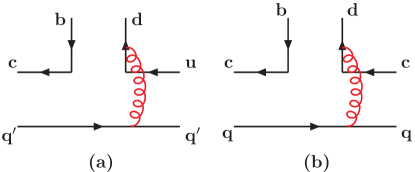
except there appears a CKM suppressed factor $V_{cd}\approx\lambda$ (see Fig.1a) for $D^{0}\bar{D}^{0}$ and $D^{+}_{s}D^{-}_{s}$ modes, the four modes have the same decay topologies. Hence, by assuming that they have similar hadronic effects, the BRs of $B^{0}\to D^{0}\bar{D}^{0}(D^{+}_{s}D^{-}_{s})$ could be estimated to be less than ${\cal O}(10^{-6})$.

To give a detailed analysis, we can include the character of each mode, governed by the meson distribution amplitudes. For simplicity, we will concentrate on the leading twist effects and take the meson wave functions to be $\Phi_{D}\propto f_{D}x(1-x)(1+0.8(1-2x))$ PQCD , $\Phi_{D_{s}}\propto f_{D_{s}}x(1-x)(1+0.3(1-2x))$ LU , $J/\Psi\propto f_{J/\Psi}x(1-x)(x(1-x)/(1-2.8x(1-x)))^{0.7}$ BC and $\Phi_{K}\propto f_{K}x(1-x)(1+0.51(1-2x)+0.3[5(1-2x)^{2}-1])$ BBKT , where $x$ is the momentum fraction of the parton inside the meson and $f_{D,D_{s},J/\Psi,K}$ are the decay constants of $D$, $D_{s}$, $J/\Psi$ and $K$ mesons, respectively. From these wave functions, we know that the maximum contributions are from $x_{0}\approx(0.35,0.43,0.5,0.5)$ for $(D,D_{s},J/\Psi,K)$. With the information, we can estimate the decay amplitudes in order of magnitude for $\bar{B}_{d}\to D^{+}_{s}K^{-}(J/\Psi D^{0})$ and $\bar{B}_{d}\to D^{0}\bar{D}^{0}(D^{+}_{s}D^{-}_{s})$ as shown in Figs. 1a and 1b with $q^{\prime}=s(c)$ and $q=u(s)$, respectively. Note that there exists a chiral suppression in the factorized parts in annihilation contributions. However, we just consider the nonfactorized effects in the estimations. Therefore, by Fig. 1 with the gluon exchange, the decay amplitude is related to the propagators of the gluon and the light quark, described by $1/(k_{2}+k_{3})^{2}/(k_{2}+k_{3})^{2}$, where $k_{2(3)}$ denote the momenta carried by the spectators. For simplicity, we have neglected the momentum carried by the light quark of the $B$ meson. By the momentum fraction, the decay amplitude could satisfy that $A\propto 1/(x_{2}x_{3})^{2}$. Hence, the relative size of the decay amplitudes could be given approximately as

$$A(D^{+}_{s}K^{-}):A(J/\Psi D^{0}):A(D^{0}\bar{D}^{0}):A(D^{+}_{s}\bar{D}^{-}_{s})\sim\frac{f_{D_{s}}f_{K}}{(x_{2}x_{3})^{2}}:\frac{f_{J/\Psi}f_{D}}{(x_{2}x_{3})^{2}}:\frac{\lambda f^{2}_{D}}{(x_{2}x_{3})^{2}}:\frac{\lambda f^{2}_{D_{s}}}{(x_{2}x_{3})^{2}}\;.$$

With the information of maximum contributions, characterized by $x_{0}$ for each mode, we get

$$A(D^{+}_{s}K^{-}):A(J/\Psi D^{0}):A(D^{0}\bar{D}^{0}):A(D^{+}_{s}\bar{D}^{-}_{s})\sim$$

$$1:\frac{f_{D}f_{J/\Psi}}{f_{D_{s}}f_{K}}\left(\frac{0.43}{0.65}\right)^{2}:\frac{\lambda f^{2}_{D}}{f_{D_{s}}f_{K}}\left(\frac{0.5\cdot 0.43}{0.35^{2}}\right)^{2}:\frac{\lambda f_{D_{s}}}{f_{K}}\left(\frac{0.5}{0.43}\right)^{2}.$$ (22)

With the kinetic effects, the ratios of BRs are roughly to be $BR(D^{+}_{s}K^{-}):BR(J/\Psi D^{0}):BR(D^{0}\bar{D}^{0}):BR(D^{+}_{s}\bar{D}^{-}_{s})\sim 1:0.25:0.39:0.16$. That is, the BRs of $\bar{B}\to D^{0}\bar{D}^{0}(D^{+}_{s}D^{-}_{s})$ could be as large as ${\cal O}(10^{-6})$, which implies that annihilation effects could be neglected in the discussions on the BR of the production for color-allowed two charmful mesons. We note that our estimations are just based on SD effects and at the level of order of magnitude. Clearly, direct experimental measurements are needed to confirm our results.

IV.2 $\alpha_{s}$, power corrections and the parametrization of Isgur-Wise function

In the HQS limit, the form factors could be related to a single Isgur-Wise function $\xi(\omega)$ by $\xi_{+}=\xi_{V}=\xi_{A_{1}}=\xi_{A_{3}}=\xi(w)$ and $\xi_{-}=\xi_{A_{2}}=0$. We now include the perturbative QCD corrections induced by hard gluon vertex corrections of $b\to c$ transitions and power corrections in orders of $1/m_{Q}$ with $Q=b$ and $c$. Consequently, the form factors can be written as

$$\xi_{i}(w)=\left\{\alpha_{i}+\beta_{i}(w)+\gamma_{i}(w)\right\}~{}\xi(w).$$ (23)

where $\xi(w)$ is the Isgur-Wise function, $\alpha_{+}=\alpha_{V}=\alpha_{A_{1}}=\alpha_{A_{3}}=1$, $\alpha_{-}=\alpha_{A_{2}}=0$ and $\beta_{i}(\omega)$ and $\gamma_{i}(\omega)$ stand for effects of $\alpha_{s}$ and power corrections, respectively. Explicitly, for the two-body decays in our study, $\omega\sim 1.3$ and the values of the other parameters are summarized as follows NeubertQCD ; NR :

$$\begin{array}[]{lll}\beta_{+}=-0.043,{}{}{}{}{}&\beta_{-}=0.069,{}{}{}{}{}&\beta_{V}=0.072,\\ \beta_{A_{1}}=-0.067,{}{}{}{}{}&\beta_{A_{2}}=-0.114,{}{}{}{}{}&\beta_{A_{3}}=-0.028,\\ \gamma_{+}=0.015,{}{}{}{}{}&\gamma_{-}=-0.122,{}{}{}{}{}&\gamma_{V}=0.224,\\ \gamma_{A_{1}}=0.027,{}{}{}{}{}&\gamma_{A_{2}}=-0.093,{}{}{}{}{}&\gamma_{A_{3}}=0.014.\end{array}$$ (28)

Clearly, the range of their effects is from few percent to 20% level. In particular, the power corrections to the form factor $\xi_{V}$ (or say $V(q^{2})$) are the largest, about 20%. The resultant is also consistent with other QCD approaches, such as the constitute quark model (CQM) MS and the light-front (LF) QCD CCH .

After taking care of the corrections, the remaining unknown is the Isgur-Wise function. To determine it, we adopt a linear parametrization to be $\xi(w)=1-\rho^{2}_{H}(w-1)$ for the transition $B\to H$, where $\rho^{2}_{H}$ is called the slope parameter. We use the BRs of semileptonic $B\to D^{(*)}\ell^{-}\bar{\nu}_{\ell}$ decays to determine $\rho^{2}_{H}$. We note that the values of $\rho^{2}_{D}$ and $\rho^{2}_{D^{*}}$ are not the same as those in $D$ and $D^{*}$ decays. In our approach, the difference is from higher orders and power corrections. Hence, with $V_{cb}=0.0416$ and $BR(B\to D^{(*)}\ell^{-}\bar{\nu}_{\ell})=2.15\pm 0.22(6.5\pm 0.5)\%$ PDG04 , we obtain $\rho^{2}_{D}=0.90\pm 0.06$ and $\rho^{2}_{D^{*}}=1.09\pm 0.05$. Since the errors of $\rho^{2}_{H}$ are small, we will only use the central values in our numerical results.

IV.3 Results for BRs and polarization fractions

To get the numerical estimations, the input values for the relevant parameters are taken to be as follows PDG04 ; NS ; CKM :

$$f_{D}=0.20,~{}~{}\ f_{D^{*}}=0.23,~{}~{}f_{D_{s}}=0.24,~{}~{}f_{D_{s}^{*}}=0.275~{}{\rm GeV};$$

$$V_{cd}=-\lambda,~{}~{}~{}~{}~{}~{}~{}~{}~{}~{}V_{cs}=1-\lambda^{2}/2,~{}~{}~{}~{}~{}~{}~{}~{}~{}V_{cb}=A\lambda^{2},$$

$$V_{td}=\lambda|V_{cb}|R_{t}e^{-i\phi_{1}},~{}~{}~{}~{}~{}V_{ts}=-A\lambda^{2},~{}~{}~{}~{}~{}V_{tb}=1,$$

$$A=0.83,~{}~{}~{}~{}~{}\lambda=0.224,~{}~{}~{}~{}~{}\phi_{1}=23.4^{\rm o},~{}~{}~{}~{}~{}R_{t}=0.91;$$

$$m_{u}=0.005,\ m_{d}=0.01,\ m_{s}=0.15,\ m_{c}=1.5,\ m_{b}=4.5~{}{\rm GeV}.$$ (29)

Note that the numerical results are insensitive to light quark masses. As to the WCs, we adopt the formulas up to one-loop corrections presented in Ref. GFA2 and set $\mu=2.5$ GeV. As mentioned early, since the nonfactorized contributions are grouped into $N^{\rm eff}_{c}$, the color number in Eq. (4) will be regarded as a variable. To display their effects, we take the values of $N^{\rm eff}_{c}=2,\;3,\;5$ and $\infty$.

By following the factorized formulas shown in Appendixes, we present the BRs with various $N^{\rm eff}_{c}$ in Tables 1, 2 and 3 for $PP$, $PV(VP)$ and $VV$ modes, respectively. In order to accord with the experimental data, our predictions of the BRs are given as the CP-averaged values. For comparisons, we also calculate the results in terms of the form factors given by the CQM and LF, which are displayed in Table 4. Since the CPAs are quite similar in different models, in Table 4 we just show the results in our approach. As to the polarization fractions, we present them in Table 5. Therein, to understand the influence of the HQS breaking effects, we separate the results to be HQS and HQS_I(II), representing the HQS results and those with $\alpha_{s}$ ($\alpha_{s}$+power) corrections, respectively.

Table 1: BRs (in unit of $10^{-3}$) for $B\to PP$ decays with $\rho^{2}_{D}=0.90$.

mode	$N^{\rm eff}_{c}=2$	$N^{\rm eff}_{c}=3$	$N^{\rm eff}_{c}=5$	$N^{\rm eff}_{c}=\infty$	Exp.
$\bar{B}^{0}\to D^{+}D_{s}^{-}$	7.26	8.25	9.06	10.46	$8\pm 3$ PDG04
$B^{-}\to D^{0}D_{s}^{-}$	7.85	8.94	9.82	11.34	$13\pm 4$ PDG04
$\bar{B}^{0}\to D^{+}D^{-}$	0.28	0.31	0.34	0.40	$0.321\pm 0.057\pm 0.048$ BELLE_DD
$B^{-}\to D^{0}D^{-}$	0.30	0.33	0.37	0.43	$0.562\pm 0.082\pm 0.065$ BELLE_DD

Table 2: BRs (in unit of $10^{-3}$) for $B\to PV(VP)$ decays with $\rho^{2}_{D^{(*)}}=0.90(1.09)$.

mode	$N^{\rm eff}_{c}=2$	$N^{\rm eff}_{c}=3$	$N^{\rm eff}_{c}=5$	$N^{\rm eff}_{c}=\infty$	Exp.
$\bar{B}^{0}\to D^{+}D_{s}^{*-}$	9.52	10.80	11.84	13.62	$10\pm 5$ PDG04
$\bar{B}^{0}\to D^{*+}D_{s}^{-}$	6.78	7.67	8.41	9.66	$10.7\pm 2.9$ PDG04
$B^{-}\to D^{0}D_{s}^{*-}$	10.35	11.73	12.87	14.79	$9\pm 4$ PDG04
$B^{-}\to D^{*0}D_{s}^{-}$	7.37	8.34	9.14	10.49	$12\pm 5$ PDG04
$\bar{B}^{0}\to D^{*+}D^{-}$	0.25	0.29	0.32	0.36
$\bar{B}^{0}\to D^{+}D^{*-}$	0.37	0.42	0.46	0.53
$\bar{B}^{0}\to D^{*+}D^{-}$	0.62	0.71	0.78	0.89	$0.93\pm 0.15$ PDG04
$~{}~{}~{}~{}~{}+D^{+}D^{*-}$
$B^{-}\to D^{0}D^{*-}$	0.40	0.45	0.50	0.57	$0.459\pm 0.072\pm 0.056$ BELLE_DD
$B^{-}\to D^{*0}D^{-}$	0.28	0.31	0.34	0.39

Table 3: BRs (in unit of $10^{-3}$) for $B\to VV$ decays with $\rho^{2}_{D^{*}}=1.09$.

mode	$N^{\rm eff}_{c}=2$	$N^{\rm eff}_{c}=3$	$N^{\rm eff}_{c}=5$	$N^{\rm eff}_{c}=\infty$	Exp.
$\bar{B}^{0}\to D^{*+}D_{s}^{*-}$	22.52	25.51	27.98	32.19	$19\pm 5$ PDG04 ;
					$18.8\pm 0.9\pm 1.7$ BABAR_DD
$B^{-}\to D^{*0}D_{s}^{*-}$	24.44	27.69	30.37	34.93	$27\pm 10$ PDG04
$\bar{B}^{0}\to D^{*+}D^{*-}$	0.87	0.91	0.99	1.14	$0.81\pm 0.08\pm 0.11$ BELLE_DD ;
					$0.87\pm 0.18$ PDG04
$B^{-}\to D^{*0}D^{*-}$	0.81	0.98	1.08	1.24

Table 4: BRs (in unit of $10^{-3}$) with $N^{\rm eff}_{c}=3$ and the form factors calculated in the CQM, LF and HQSC, while the CPA is only shown in our approach (HQSC).

Mode	CQM	LF	HQSC	$A_{CP}(\%)$
$\bar{B}^{0}\to D^{+}D_{s}^{-}$	9.70	10.33	8.25	$-0.2$
$B^{-}\to D^{0}D_{s}^{-}$	10.58	11.26	8.94	$-0.2$
$\bar{B}^{0}\to D^{+}D^{-}$	0.38	0.40	0.31	$2.5$
$B^{-}\to D^{0}D^{-}$	0.42	0.44	0.33	$2.5$
$\bar{B}^{0}\to D^{+}D_{s}^{*-}$	12.49	11.42	10.80	$-0.1$
$\bar{B}^{0}\to D^{*+}D_{s}^{-}$	9.19	8.50	7.67	$0.0$
$B^{-}\to D^{0}D_{s}^{*-}$	13.65	12.47	11.73	$-0.1$
$B^{-}\to D^{*0}D_{s}^{-}$	10.02	9.27	8.34	$0.0$
$\bar{B}^{0}\to D^{*+}D^{-}$	0.36	0.33	0.29	$0.2$
$\bar{B}^{0}\to D^{+}D^{*-}$	0.37	0.45	0.42	$0.9$
$\bar{B}^{0}\to D^{*+}D^{-}$	0.73	0.78	0.71	$0.6$
$~{}~{}~{}~{}~{}+D^{+}D^{*-}$
$B^{-}\to D^{0}D^{*-}$	0.54	0.49	0.45	$0.9$
$B^{-}\to D^{*0}D^{-}$	0.39	0.36	0.31	$0.2$
$\bar{B}^{0}\to D^{*+}D_{s}^{*-}$	28.78	27.09	25.51	$-0.1$
$B^{-}\to D^{*0}D_{s}^{*-}$	31.37	29.52	27.69	$-0.1$
$\bar{B}^{0}\to D^{*+}D^{*-}$	1.06	0.99	0.91	$0.9$
$B^{-}\to D^{*0}D^{*-}$	1.16	1.08	0.98	$0.9$

Table 5: Polarization fractions in various QCD approaches, where HQS_I and HQS_II denote the results with $\alpha_{s}$ and $\alpha_{s}$ + power corrections, respectively.

Mode	CQM	LF	HQS	HQSI	HQSII
$\bar{B}^{0}\to D^{*-}D_{s}^{*+}$	$R_{0}=0.523$	$R_{0}=0.512$	$R_{0}=0.515$	$R_{0}=0.517$	$R_{0}=0.512$
	$R_{\perp}=0.069$	$R_{\perp}=0.077$	$R_{\perp}=0.055$	$R_{\perp}=0.070$	$R_{\perp}=0.093$
$B^{-}\to D^{*0}D_{s}^{*-}$	$R_{0}=0.524$	$R_{0}=0.512$	$R_{0}=0.515$	$R_{0}=0.517$	$R_{0}=0.512$
	$R_{\perp}=0.070$	$R_{\perp}=0.078$	$R_{\perp}=0.055$	$R_{\perp}=0.070$	$R_{\perp}=0.093$
$\bar{B}^{0}\to D^{*+}D^{*-}$	$R_{0}=0.547$	$R_{0}=0.535$	$R_{0}=0.538$	$R_{0}=0.540$	$R_{0}=0.535$
	$R_{\perp}=0.069$	$R_{\perp}=0.077$	$R_{\perp}=0.055$	$R_{\perp}=0.070$	$R_{\perp}=0.092$
$B^{-}\to D^{*0}D^{*-}$	$R_{0}=0.547$	$R_{0}=0.535$	$R_{0}=0.538$	$R_{0}=0.541$	$R_{0}=0.535$
	$R_{\perp}=0.069$	$R_{\perp}=0.077$	$R_{\perp}=0.055$	$R_{\perp}=0.070$	$R_{\perp}=0.092$

We now present our discussions on the results as follows:

(1) The non-factorizable contributions are not dominant for color-allowed two charmed-meson decays. According to the classification in Refs. GFA1 ; GFA2 , the decay modes displaced in Tables 1, 2 and 3 belong to class I, which are dominated by the external $W$-emission. The leading decay amplitudes are proportional to the effective coefficient $a_{1}$, which is stable against the variation of $N_{c}^{\rm eff}$. Thus, the predicted branching ratios are insensitive to $N_{c}^{\rm eff}$. This means that annihilation contributions and FSIs, neglected in the GFA, are sub-leading contributions. On the other hand, by varying $N_{c}^{\rm eff}$ from $3$ to $2$, or $3$ to $\infty$, the branching ratios change by about 10-20%, which should be the same order as annihilation and FSI effects. From Tables 1, 2 and 3, there are no obvious deviations of the theoretical predictions from the experimental data within the present errors. It is also interesting to note that $N_{c}^{\rm eff}=\infty$ is not excluded by experiments if considering the uncertainties of decay constants and from factors. Thus, the large $N_{c}$ limit as a mechanism of factorization is not disfavored yet.

(2) The main uncertainties of theory come from the decay constants and form factors. Because the decay amplitudes are proportional to decay constants, it is clear that the theoretical predictions can be changed with different values of the decay constants. For instance, the branching ratio is ${\rm BR(our~{}result)}\times\left(\frac{f_{D_{s}}}{0.24}\right)^{2}$ for $\bar{B}^{0}\to D^{+}D_{s}^{-}$. The recent experiment ${\rm BR}(\bar{B}^{0}\to D^{*+}D_{s}^{*-})=18.8\pm 0.9\pm 1.7$ seems to favor a lower $f_{D_{s}^{*}}\approx 0.24$ than our choice of $0.275$. However, this point has to be checked by other processes. For the form factors, the predictions of BRs in our approach are slightly lower than those in other two approaches (CQM and LF). The present experiment data can not distinguish which model is more preferred. More precise data are necessary. Another place to test different approaches is through the transverse polarization $R_{\perp}$. From Table 5, $R_{\perp}$ is predicted to be $0.07,~{}0.08$ and $0.09$ in the CQM, LF and HQET, respectively. The larger prediction in the HQET is due to $\alpha_{s}$ corrections. Except the model-dependent calculation of power corrections in different approaches, one advantage of the HQET is that it permits the calculations of perturbative QCD corrections systematically.

(3) The penguin effects can not be neglected in $B\to PP$ decays. By using the decay amplitudes in Appendixes, the definitions of hadronic effects in Eqs. (9) and (10) and the condition of $\varepsilon_{i}(p_{i})\cdot p_{i}=0$, we know that the effects of penguin ($P$) to tree ($T$) level, denoted by $P/T$, for $PP$, $VP$ and $VV$ modes are proportional to $(a^{\rm eff(c)}_{4}+2a^{\rm eff(c)}_{6}{\cal R})/a^{\rm eff}_{1}$, $(a^{\rm eff(c)}_{4}-2a^{\rm eff(c)}_{6}{\cal R^{\prime}})/a^{\rm eff}_{1}$ and $a^{\rm eff(c)}_{4}/a^{\rm eff}_{1}$, respectively, where ${\cal R}=m^{2}_{D}/[(m_{c}+m_{d})(m_{b}-m_{c})]$ and ${\cal R^{\prime}}=m^{2}_{D}/[(m_{c}+m_{d})(m_{b}+m_{c})]$ and the CKM matrix elements have been canceled due to $|V_{tb}V^{*}_{ts}|\approx|V_{cb}V^{*}_{cs}|$ and $|V_{tb}V^{*}_{td}|\approx|V_{cb}V^{*}_{cd}|$. The situations in the $PV$ modes are the same as those in the $VV$ modes due to the vector meson being factorized out from the $B\to P$ transition. Since the WCs $a^{\rm eff(c)}_{4}$ and $a^{\rm eff(c)}_{6}$ have the same sign, we see clearly that penguin effects in the $PP$ modes are larger than those in the $VV$ modes; however, due to the cancelation between $a^{\rm eff(c)}_{4}$ and $a^{\rm eff(c)}_{6}$, penguin effects could be neglected in $B\to VP$ decays. Hence, the ratios $|P/T|$ for $PP$, $VP$ and $VV(PV))$ are around $15\%$, $0\%$ and $4\%$, respectively. For the $PP,VV(PV)$ modes, our predictions are consistent with the results in Refs. CY ; KKLM . Note that an 4% penguin contribution was obtained for the $VP$ modes in CY . The difference is due to that they used a lower charm quark mass ($m_{c}=0.95~{}{\rm GeV}$) than ours. For all the decay modes, the electroweak penguin contributions can be negligible (less than 1%).

(4) Without FSIs, we find that the BRs in the neutral and charged modes have the following relationships:

$$\frac{1}{\tau_{B^{0}}}BR(D^{(*)+}D^{(*)-}_{s}) \approx \frac{1}{\tau_{B^{+}}}BR(D^{(*)0}D^{(*)-}_{s}),$$

$$\frac{1}{\tau_{B^{0}}}BR(D^{(*)+}D^{(*)-}) \approx \frac{1}{\tau_{B^{+}}}BR(D^{(*)0}D^{(*)-}).$$

In addition, the decays with nonstrangeness charmed mesons are Cabibbo-suppressed compared to the decays with the $D^{(*)}_{s}$ emission and they satisfy

$$BR(B\to D^{(*)}D^{(*)})\approx\frac{f^{2}_{D^{(*)}}}{f^{2}_{D^{(*)}_{s}}}\lambda^{2}BR(B\to D^{(*)}D^{(*)}_{s}).$$ (30)

Clearly, if large deviations from the equalities in Eq. (30) are observed in experiments, they should arise from FSIs. Of course, if the BRs of $\bar{B}^{0}\to D^{(*)0}\bar{D}^{(*)0}$ and $\bar{B}^{0}\to D^{(*)+}_{s}D^{(*)-}_{s}$ with ${\cal O}(10^{-4})$ are seen, it will be another hint for FSIs EFP .

(5) For the decay amplitude, we write

$$A=T+Pe^{i\theta_{W}}e^{i\delta},$$ (31)

where $T$ and $P$ represent tree and penguin amplitudes, and we have chosen the convention such that $T$ and $P$ are real numbers and $\theta_{W}$ and $\delta$ are the CP weak and strong phases, respectively. From Eq. (13), the CPA can be described by

$$A_{CP}={2(P/T)\sin\delta\sin\theta_{W}\over 1+(P/T)^{2}+2(P/T)\cos\delta\cos\theta_{W}}.$$ (32)

According to the discussions in (1), the maximum CPAs in $PP$, $PV$ and $VV(VP)$ are expected to be around $26\%$, $0\%$ and $8\%$, respectively. However, in $B\to D^{(*)}D^{(*)}$ decays, due to $|\theta_{W}|=|\phi_{1}|$, if we take $\delta=90^{o}$ and $\phi=23.4^{o}$, the maximum CPAs for $PP$ and $VV(VP)$ modes are $10.3\%$ and $1.6\%$, respectively. Clearly, in the SM, the CPA with ${\cal O}(10\%)$ can be reached in $B\to DD$ decays. Due to the associated CKM matrix element being $V_{ts}\approx-A\lambda^{2}$, there are no CPAs in $B\to D^{(*)}D^{(*)}_{s}$ decays. In the GFA, since the strong phases mainly arise from the one-loop corrections which are usually small, our results on CPAs, shown in Table 4, are all at a few percent level. Therefore, if the CPAs of ${\cal O}(10\%)$ are found in $\bar{B}^{0}\to D^{+}D^{-}$ and $\bar{B}^{+}\to D^{0}D^{-}$ decays, we can conclude the large effects of the strong phase are from FSIs.

(6) As discussed before, we know that in two charmful decays the polarization fractions satisfy $R_{\perp}<<R_{0}\sim R_{\parallel}$. The current experimental data are: $R_{0}=0.52\pm 0.05$ PDG04 for $B^{0}\to D^{*+}D_{s}^{*-}$ and $R_{0}=0.57\pm 0.08\pm 0.02$, $R_{\perp}=0.19\pm 0.08\pm 0.01$ BELLE_DD and $R_{\perp}=0.063\pm 0.055\pm 0.009$ BABAR_DD for $B^{0}\to D^{*+}D^{*-}$. We can see that the experimental measurements support the power-law relation. To estimate how large $R_{\perp}$ can be in theory, we use the relationship in Eq. (21) and the form factors in Eq. (7) and we obtain

$$\frac{R_{\perp}}{R_{\perp}^{HQS}}\approx\left[\frac{1+\beta_{V}+\gamma_{V}}{1+\beta_{A_{1}}+\gamma_{A_{1}}}\right]^{2}.$$ (33)

With the values in Eq. (28) and $R^{HQS}_{\perp}=0.055$, we get $R_{\perp}\approx 10\%$. The detailed numerical values can be found in Table 5. Interestingly, for the $\bar{B}^{0}\to D^{*+}D^{*-}$ decay, the estimated result is close to the upper limit of $R_{\perp}=0.063\pm 0.055\pm 0.009$ observed by BABAR BABAR_DD but close to the lower limit of $R_{\perp}=0.19\pm 0.08\pm 0.01$ observed by BELLE BELLE_DD . We note that our results are different from the PQCD predictions in which $R_{\perp}\sim 0.06$ LM . From our results, we can conjecture that if large $R_{\perp}$, say around $20\%$, is observed, large contributions should arise from FSIs.

V Conclusions

We have presented a detailed study of B decaying into two charmed-mesons in the generalized factorization approach. The penguin contributions have also been taken into account. If the final states are both pseudoscalar mesons, the ratio of penguin and tree contributions is about 10% in the decay amplitude. The direct CP violating asymmetries have been estimated to be a few percent. For the $B^{0}\to D^{*+}D^{-},~{}D^{+}D^{*-},~{}D^{*+}D^{*-}$ decays, the “penguin pollution” is weaker than that in the $D^{+}D^{-}$ mode. Thus, these modes provide cleaner places to cross-check the value of $sin2\beta$ measured in the $B^{0}\to J/\psi K$ decays. The weak annihilation contributions have been found to be small. We have proposed to test the annihilation effects in annihilation-dominated processes of $B^{0}\to D^{(*)0}\bar{D}^{(*)0}$ and $D^{(*)+}_{s}D^{(*)-}_{s}$.

We have performed a comprehensive test of the factorization in the heavy-heavy B decays. The predictions of branching ratios in theory are consistent with the experimental data within the present level. The variations of branching ratios with the effective color number $N_{c}^{\rm eff}$ show that the soft FSIs are not dominant. However, we cannot make the conclusion that they are negligible. Their effects can be of order 10-20% for branching ratios as indicated from the variation of $N_{c}^{\rm eff}$. Since the soft divergences are not canceled in the non-factorizable corrections, this may indicate that the strong interactions at low energy either become weak or are suppressed by some unknown parameters (such as $N_{c}$ in the large $N_{c}$ theory). If the factorization is still a working concept in the heavy-heavy decays, there must be some non-perturbative mechanisms which prefer the factorization of a large-size charmed-meson from an environment of “soft cloud”. A relevant comment on the necessity of non-perturbative QCD justification can be found in LLW .

The polarization structure in the heavy-heavy decays has shown that the transverse perpendicular polarization fraction $R_{\perp}$ is the smallest while the other two are comparable in size. This structure follows from the QCD dynamics in the heavy quark limit. We have found one relation between the transverse perpendicular polarization fraction and the ratios of form factors, in particular $V(q^{2})/A_{1}(q^{2})$. The corrections to the heavy quark limit give an enhancement of $R_{\perp}$ from 0.055 to about 0.09. Since the FSIs are not significant, we do not expect that FSIs can change our prediction of $R_{\perp}$ substantially. If future measurements confirm $R_{\perp}\sim 0.2$ as the recent measurement by BELLE, it will be difficult to explain within the HQET and the factorization hypothesis.

In conclusion, our study has shown that the factorization works well in B meson heavy-heavy decays at present. More precise experimental data are desired to give a better justification. For theory, to explain the mechanism of factorization in the heavy-heavy decays is of high interest. The measurement of the transverse perpendicular polarization provides important information on the size of the heavy quark symmetry breaking or the possibility of large non-factorizable effects.

Acknowledgments
We thank Hai-Yang Cheng and Yu-Kuo Hsiao for many valuable discussions. This work is supported in part by the National Science Council of R.O.C. under Grant #s: NSC-93-2112-M-006-010 and NSC-93-2112-M-007-014.

$B\to PP$ decays

$$A(\bar{B}^{0}\to D^{+}D^{-}_{s}) = V_{cb}V^{*}_{cs}a^{\rm eff}_{1}X^{(BD,D_{s})}_{1}-V_{tb}V^{*}_{ts}\left[\left(a^{\rm eff(c)}_{4}X^{(BD,D_{s})}_{1}-2a^{\rm eff(c)}_{6}X^{(BD,D_{s})}_{2}\right)\right.$$ (34)

$$+\left.\left(a^{\rm eff(d)}_{4}Y^{(B,DD_{s})}_{1}-2a^{\rm eff(d)}_{6}Y^{(B,DD_{s})}_{3}\right)\right],$$

$$A(\bar{B}^{0}\to D^{+}_{s}D^{-}_{s}) = V_{cb}V^{*}_{cd}a^{\rm eff}_{2}Y^{(B,D_{s}D_{s})}_{1}-V_{tb}V^{*}_{td}\left[(a^{\rm eff(s)}_{3}+a^{\rm eff(c)}_{3})Y^{(B,D_{s}D_{s})}_{1}\right.$$ (35)

$$+\left.(a^{\rm eff(s)}_{5}+a^{\rm eff(c)}_{5})Y^{(B,D_{s}D_{s})}_{2}\right],$$

$$A(B^{-}\to D^{0}D^{-}_{s}) = V_{cb}V^{*}_{cs}a^{\rm eff}_{1}X^{(BD,D_{s})}_{1}+V_{ub}V^{*}_{us}a^{\rm eff}_{1}Y^{(B,DD_{s})}_{1}-V_{tb}V^{*}_{ts}\left[\left(a^{\rm eff(c)}_{4}X^{(BD,D_{s})}_{1}\right.\right.$$ (36)

$$-\left.\left.2a^{\rm eff(c)}_{6}X^{(BD,D_{s})}_{2}\right)+\left(a^{\rm eff(u)}_{4}Y^{(B,DD_{s})}_{1}-2a^{\rm eff(u)}_{6}Y^{(B,DD_{s})}_{3}\right)\right],$$

$$A(\bar{B}^{0}\to D^{+}D^{-}) = V_{cb}V^{*}_{cd}\left[a^{\rm eff}_{1}X^{(BD,D)}_{1}+a^{\rm eff}_{2}Y^{(B,DD)}_{1}\right]-V_{tb}V^{*}_{td}\left[\left(a^{\rm eff(c)}_{4}X^{(BD,D)}_{1}\right.\right.$$ (37)

$$-\left.2a^{\rm eff(c)}_{6}X^{(BD,D)}_{2}\right)+(a^{\rm eff(d)}_{4}+a^{\rm eff(d)}_{3}+a^{\rm eff(c)}_{3})Y^{(B,DD)}_{1}$$

$$+\left.(a^{\rm eff(d)}_{5}+a^{\rm eff(c)}_{5})Y^{(B,DD)}_{2}-2a^{\rm eff(d)}_{6}Y^{(B,DD)}_{3}\right],$$

$$A(\bar{B}^{0}\to D^{0}\bar{D}^{0}) = \left(V_{cb}V^{*}_{cd}+V_{ub}V^{*}_{ud}\right)a^{\rm eff}_{2}Y^{(B,DD)}_{1}-V_{tb}V^{*}_{td}\left[(a^{\rm eff(u)}_{3}+a^{\rm eff(c)}_{3})Y^{(B,DD)}_{1}\right.$$ (38)

$$+\left.(a^{\rm eff(u)}_{5}+a^{\rm eff(c)}_{5})Y^{(B,DD)}_{2}\right],$$

$$A(B^{-}\to D^{0}D^{-}) = V_{cb}V^{*}_{cd}a^{\rm eff}_{1}X^{(BD,D)}_{1}+V_{ub}V^{*}_{ud}a^{\rm eff}_{1}Y^{(B,DD)}_{1}-V_{tb}V^{*}_{td}\left[\left(a^{\rm eff(c)}_{4}X^{(BD,D)}_{1}\right.\right.$$ (39)

$$-\left.\left.2a^{\rm eff(c)}_{6}X^{(BD,D)}_{2}\right)+a^{\rm eff(d)}_{4}Y^{(B,DD)}_{1}-2a^{\rm eff(d)}_{6}Y^{(B,DD)}_{3}\right].$$

Appendix A $B\to PV(VP)$ decays

$$A(\bar{B}^{0}\to D^{+}D^{*-}_{s}) = V_{cb}V^{*}_{cs}a^{\rm eff}_{1}X^{(BD,D^{*}_{s})}_{1}-V_{tb}V^{*}_{ts}\left[a^{\rm eff(c)}_{4}X^{(BD,D^{*}_{s})}_{1}\right.$$ (40)

$$+\left.\left(a^{\rm eff(d)}_{4}Y^{(B,DD^{*}_{s})}_{1}-2a^{\rm eff(d)}_{6}Y^{(B,DD^{*}_{s})}_{3}\right)\right],$$

$$A(\bar{B}^{0}\to D^{*+}D^{-}_{s}) = V_{cb}V^{*}_{cs}a^{\rm eff}_{1}X^{(BD^{*},D_{s})}_{1}-V_{tb}V^{*}_{ts}\left[\left(a^{\rm eff(c)}_{4}X^{(BD^{*},D_{s})}_{1}-2a^{\rm eff(c)}_{6}X^{(BD^{*},D_{s})}_{2}\right)\right.$$ (41)

$$+\left.\left(a^{\rm eff(d)}_{4}Y^{(B,D^{*}D_{s})}_{1}-2a^{\rm eff(d)}_{6}Y^{(B,D^{*}D_{s})}_{3}\right)\right],$$

$$A(\bar{B}^{0}\to D^{+}_{s}D^{*-}_{s}) = V_{cb}V^{*}_{cd}a^{\rm eff}_{2}Y^{(B,D_{s}D^{*}_{s})}_{1}-V_{tb}V^{*}_{td}\left[(a^{\rm eff(s)}_{3}+a^{\rm eff(c)}_{3})Y^{(B,D_{s}D^{*}_{s})}_{1}\right.$$ (42)

$$+\left.(a^{\rm eff(s)}_{5}+a^{\rm eff(c)}_{5})Y^{(B,D_{s}D^{*}_{s})}_{2}\right],$$

$$A(\bar{B}^{0}\to D^{*+}_{s}D^{-}_{s}) = V_{cb}V^{*}_{cd}a^{\rm eff}_{2}Y^{(B,D^{*}_{s}D_{s})}_{1}-V_{tb}V^{*}_{td}\left[(a^{\rm eff(s)}_{3}+a^{\rm eff(c)}_{3})Y^{(B,D^{*}_{s}D_{s})}_{1}\right.$$ (43)

$$=\left.(a^{\rm eff(s)}_{5}+a^{\rm eff(c)}_{5})Y^{(B,D^{*}_{s}D_{s})}_{2}\right],$$

$$A(B^{-}\to D^{0}D^{*-}_{s}) = V_{cb}V^{*}_{cs}a^{\rm eff}_{1}X^{(BD,D^{*}_{s})}_{1}+V_{ub}V^{*}_{us}a^{\rm eff}_{1}X^{(B,DD^{*}_{s})}_{1}-V_{tb}V^{*}_{ts}\left[\left(a^{\rm eff(c)}_{4}X^{(BD,D^{*}_{s})}_{1}\right.\right.$$ (44)

$$+\left.\left(a^{\rm eff(u)}_{4}Y^{(B,DD^{*}_{s})}_{1}-2a^{\rm eff(u)}_{6}Y^{(B,DD^{*}_{s})}_{3}\right)\right],$$

$$A(B^{-}\to D^{*0}D^{-}_{s}) = V_{cb}V^{*}_{cs}a^{\rm eff}_{1}X^{(BD^{*},D_{s})}_{1}+V_{ub}V^{*}_{us}a^{\rm eff}_{1}Y^{(B,D^{*}D_{s})}_{1}-V_{tb}V^{*}_{ts}\left[\left(a^{\rm eff(c)}_{4}X^{(BD^{*},D_{s})}_{1}\right.\right.$$ (45)

$$-\left.\left.2a^{\rm eff(c)}_{6}X^{(BD^{*},D_{s})}_{2}\right)+\left(a^{\rm eff(u)}_{4}Y^{(B,D^{*}D_{s})}_{1}-2a^{\rm eff(u)}_{6}Y^{(B,D^{*}D_{s})}_{3}\right)\right],$$

$$A(\bar{B}^{0}\to D^{+}D^{*-}) = V_{cb}V^{*}_{cd}\left[a^{\rm eff}_{1}X^{(BD,D^{*})}_{1}+a^{\rm eff}_{2}Y^{(B,DD^{*})}_{1}\right]-V_{tb}V^{*}_{td}\left[a^{\rm eff(c)}_{4}X^{(BD,D^{*})}_{1}\right.$$ (46)

$$+(a^{\rm eff(d)}_{4}+a^{\rm eff(d)}_{3}+a^{\rm eff(c)}_{3})Y^{(B,DD^{*})}_{1}+(a^{\rm eff(d)}_{5}+a^{\rm eff(c)}_{5})Y^{(B,DD^{*})}_{2}$$

$$-\left.2a^{\rm eff(d)}_{6}Y^{(B,DD^{*})}_{3}\right],$$

$$A(\bar{B}^{0}\to D^{*+}D^{-}) = V_{cb}V^{*}_{cd}\left[a^{\rm eff}_{1}X^{(BD^{*},D)}_{1}+a^{\rm eff}_{2}Y^{(B,D^{*}D)}_{1}\right]-V_{tb}V^{*}_{td}\left[\left(a^{\rm eff(c)}_{4}X^{(BD^{*},D)}_{1}\right.\right.$$ (47)

$$-\left.2a^{\rm eff(c)}_{6}X^{(BD^{*},D)}_{2}\right)+(a^{\rm eff(d)}_{4}+a^{\rm eff(d)}_{3}+a^{\rm eff(c)}_{3})Y^{(B,D^{*}D)}_{1}$$

$$+\left.(a^{\rm eff(d)}_{5}+a^{\rm eff(c)}_{5})Y^{(B,D^{*}D)}_{2}-2a^{\rm eff(d)}_{6}Y^{(B,D^{*}D)}_{3}\right],$$

$$A(\bar{B}^{0}\to D^{0}\bar{D}^{*0}) = \left(V_{cb}V^{*}_{cd}+V_{ub}V^{*}_{ud}\right)a^{\rm eff}_{2}Y^{(B,DD^{*})}_{1}-V_{tb}V^{*}_{td}\left[(a^{\rm eff(u)}_{3}+a^{\rm eff(c)}_{3})Y^{(B,DD^{*})}_{1}\right.$$ (48)

$$+\left.(a^{\rm eff(u)}_{5}+a^{\rm eff(c)}_{5})Y^{(B,DD^{*})}_{2}\right],$$

$$A(\bar{B}^{0}\to D^{*0}\bar{D}^{0}) = \left(V_{cb}V^{*}_{cd}+V_{ub}V^{*}_{ud}\right)a^{\rm eff}_{2}Y^{(B,D^{*}D)}_{1}-V_{tb}V^{*}_{td}\left[(a^{\rm eff(u)}_{3}+a^{\rm eff(c)}_{3})Y^{(B,D^{*}D)}_{1}\right.$$ (49)

$$+\left.(a^{\rm eff(u)}_{5}+a^{\rm eff(c)}_{5})Y^{(B,D^{*}D)}_{2}\right],$$

$$A(B^{-}\to D^{0}D^{*-}) = V_{cb}V^{*}_{cd}a^{\rm eff}_{1}X^{(BD,D^{*})}_{1}+V_{ub}V^{*}_{ud}a^{\rm eff}_{1}Y^{(B,DD^{*})}_{1}-V_{tb}V^{*}_{td}\left[a^{\rm eff(c)}_{4}X^{(BD,D^{*})}_{1}\right.$$ (50)

$$+\left.a^{\rm eff(d)}_{4}Y^{(B,DD^{*})}_{1}-2a^{\rm eff(d)}_{6}Y^{(B,DD^{*})}_{3}\right],$$

$$A(B^{-}\to D^{*0}D^{-}) = V_{cb}V^{*}_{cd}a^{\rm eff}_{1}X^{(BD^{*},D)}_{1}+V_{ub}V^{*}_{ud}a^{\rm eff}_{1}Y^{(B,D^{*}D)}_{1}-V_{tb}V^{*}_{td}\left[\left(a^{\rm eff(c)}_{4}X^{(BD^{*},D)}_{1}\right.\right.$$ (51)

$$-\left.\left.2a^{\rm eff(c)}_{6}X^{(BD^{*},D)}_{2}\right)+a^{\rm eff(d)}_{4}Y^{(B,D^{*}D)}_{1}-2a^{\rm eff(d)}_{6}Y^{(B,D^{*}D)}_{3}\right].$$

Appendix B $B\to VV$ decays

$$A(\bar{B}^{0}\to D^{*+}D^{*-}_{s}) = V_{cb}V^{*}_{cs}a^{\rm eff}_{1}X^{(BD^{*},D^{*}_{s})}-V_{tb}V^{*}_{ts}\left[a^{\rm eff(c)}_{4}X^{(BD^{*},D^{*}_{s})}_{1}\right.$$ (52)

$$+\left.\left(a^{\rm eff(d)}_{4}Y^{(B,D^{*}D^{*}_{s})}_{1}-2a^{\rm eff(d)}_{6}Y^{(B,D^{*}D^{*}_{s})}_{3}\right)\right],$$

$$A(\bar{B}^{0}\to D^{*+}_{s}D^{*-}_{s}) = V_{cb}V^{*}_{cd}a^{\rm eff}_{2}Y^{(B,D^{*}_{s}D^{*}_{s})}_{1}-V_{tb}V^{*}_{td}\left[(a^{\rm eff(s)}_{3}+a^{\rm eff(c)}_{3})Y^{(B,D^{*}_{s}D^{*}_{s})}_{1}\right.$$ (53)

$$+\left.(a^{\rm eff(s)}_{5}+a^{\rm eff(c)}_{5})Y^{(B,D^{*}_{s}D^{*}_{s})}_{2}\right],$$

$$A(B^{-}\to D^{*0}D^{*-}_{s}) = V_{cb}V^{*}_{cs}a^{\rm eff}_{1}X^{(BD^{*},D^{*}_{s})}+V_{ub}V^{*}_{us}a^{\rm eff}_{1}Y^{(B,D^{*}D^{*}_{s})}_{1}-V_{tb}V^{*}_{ts}\left[a^{\rm eff(c)}_{4}X^{(BD^{*},D^{*}_{s})}_{1}\right.$$ (54)

$$+\left.\left(a^{\rm eff(u)}_{4}Y^{(B,D^{*}D^{*}_{s})}_{1}-2a^{\rm eff(u)}_{6}Y^{(B,D^{*}D^{*}_{s})}_{3}\right)\right],$$

$$A(\bar{B}^{0}\to D^{*+}D^{*-}) = V_{cb}V^{*}_{cd}\left[a^{\rm eff}X^{(BD^{*},D^{*})}+a^{\rm eff}_{2}Y^{(B,D^{*}D^{*})}_{1}\right]-V_{tb}V^{*}_{td}\left[\left(a^{\rm eff(c)}_{4}X^{(BD^{*},D^{*})}\right.\right.$$ (55)

$$+(a^{\rm eff(d)}_{4}+a^{\rm eff(d)}_{3}+a^{\rm eff(c)}_{3})Y^{(B,D^{*}D^{*})}_{1}+(a^{\rm eff(d)}_{5}+a^{\rm eff(c)}_{5})Y^{(B,D^{*}D^{*})}_{2}$$

$$\left.-2a^{\rm eff(d)}_{6}Y^{(B,D^{*}D^{*})}_{3}\right],$$

$$A(\bar{B}^{0}\to D^{*0}\bar{D}^{*0}) = \left(V_{cb}V^{*}_{cd}+V_{ub}V^{*}_{ud}\right)a^{\rm eff}_{2}Y^{(B,D^{*}D^{*})}_{1}-V_{tb}V^{*}_{td}\left[(a^{\rm eff(u)}_{3}+a^{\rm eff(c)}_{3})Y^{(B,D^{*}D^{*})}_{1}\right.$$ (56)

$$+\left.(a^{\rm eff(u)}_{5}+a^{\rm eff(c)}_{5})Y^{(B,D^{*}D^{*})}_{2}\right],$$

$$A(B^{-}\to D^{*0}D^{*-}) = V_{cb}V^{*}_{cd}a^{\rm eff}X^{(BD^{*},D^{*})}+V_{ub}V^{*}_{ud}a^{\rm eff}_{1}Y^{(B,D^{*}D^{*})}_{1}-V_{tb}V^{*}_{td}\left[a^{\rm eff(c)}_{4}X^{(BD^{*},D^{*})}\right.$$ (57)

$$\left.+a^{\rm eff(d)}_{4}Y^{(B,DD)}_{1}-2a^{\rm eff(d)}_{6}Y^{(B,DD)}_{3}\right].$$

References

• (1) A.I. Sanda, Z.Z. Xing, Phys. Rev. D56, 341 (1997); Z.Z. Xing, ibid. 61, 014010 (1999).
• (2) Particle Data Group 2004, S. Eidelman et al., Phys.Β Lett.Β B 592, 1 (2004).
• (3) BELLE Collaboration, H. Miyake et al., arXiv: hep-ex/0501037; G. Majumder et al., arXiv: hep-ex/0502038.
• (4) BABAR Collaboration, B. Aubert et al., Phys.Β Rev.Β Lett.Β 91, 131801 (2003); arXiv: hep-ex/0502041.
• (5) J. Bjorken, Nucl.Β Phys.Β B (Proc.Β Suppl.) 11, 325 (1989).
• (6) M. Beneke, G. Buchalla, M. Neubert, C.T. Sachrajda, Phys.Β Rev.Β Lett.Β 83, 1914 (1999); Nucl.Β Phys.Β B 591, 313 (2000).
• (7) C.W. Bauer, D. Pirjol, I.W. Stewart Phys.Β Rev.Β Lett.Β 87, 201806 (2001); C.W. Bauer, Dan Pirjol, I.Z. Rothstein, I.W. Stewart, Phys.Β Rev.Β D70, 054015 (2004).
• (8) A.J. Buras, J.M. Gerard, R. Ruckl, Nucl.Β Phys.Β B 268, 16 (1986).
• (9) M. Bauer, B. Stech and M. Wirbel, Z.Β Phys.Β C 34, 103 (1987).
• (10) A. Ali, G. Kramer, C.D. Lu, Phys.Β Rev.Β D58, 094009 (1998).
• (11) Y.H. Chen, H.Y. Cheng, B. Tseng, K.C. Yang, Phys.Β Rev.Β D60, 094014 (1999).
• (12) Y.Y. Keum, H.N. Li, A.I. Sanda, Phys. Rev. D 63, 054008 (2001); C.D. Lu, K. Ukai, M.Z. Yang, Phys.Β Rev.Β D63, 074009 (2001).
• (13) H.Y. Cheng, C.K. Chua, A. Soni, Phys. Rev. D 71, 014030 (2005).
• (14) BABAR Collaboration, B. Aubert et al., Phys. Rev. Lett. 87, 241801 (2001); hep-ex/0408017.
• (15) BELLE Collaboration, K. F. Chen, et al., hep-ex/0503013.
• (16) H.N. Li and S. Mishima, Phys. Rev. D 71, 054025 (2005).
• (17) For a review, see M. Neubert, Phys. Rept. 245, 259 (1994).
• (18) M. Neubert, Phys.Β Rev.Β D46, 2212 (1991).
• (19) M. Neubert, V. Rieckert, Nucl.Β Phys.Β B 382, 97 (1992).
• (20) Z. Luo and J.L. Rosner, Phys.Β Rev.Β D64, 094001 (2001).
• (21) G. Buchalla, A.J. Buras, M.E. Lautenbacher, Rev. Mod. Phys. 68, 1125 (1996).
• (22) BABAR Collaboration, B. Aubert et al., arXiv: hep-ex/0503021; BELLE Collaboration, L.M. Zhang et al., arXiv: hep-ex/0503037.
• (23) Y.Y. Keum, T. Kurimoto, H.N. Li, C.D. Lu, A.I. Sanda, Phys. Rev. D 69, 094018 (2004).
• (24) Y. Li, C.D. Lu, Z.J. Xiao, J. Phys. G 31, 273 (2005).
• (25) A.E. Bondar, V.L. Chernyak, Phys. Lett. B 612, 215 (2005).
• (26) P. Ball, V.M. Braun, Y. Koike, K. Tanaka, Nucl.Β Phys.Β B 529, 323 (1998).
• (27) D. Melikhov, B. Stech, Phys. Rev. D 62, 014006 (2000).
• (28) H.Y. Cheng, C.K. Chua, C.W. Hwang, Phys. Rev. D 69, 074025 (2004).
• (29) M. Neubert, B. Stech, Adv. Ser. Direct. High Energy Phys. 15, 294 (1998), arXiv: hep-ph/9705292.
• (30) M. Battaglia et al., arXiv: hep-ph/0304132.
• (31) H.Y. Cheng, K.C. Yang, Phys.Β Rev.Β D62, 054029 (2000).
• (32) C.S. Kim, Y. Kwon, J. Lee, W. Namgung, Phys. Rev. D 65, 097503 (2002).
• (33) J.O. Eeg, S. Fajfer, A. Prapotnik, arXiv: hep-ph/0501031.
• (34) Z. Ligeti, M.E. Luke, M.B. Wise, Phys.Β Lett.Β B 507, 142 (2001).