Full one-loop supersymmetric electroweak corrections to $t\bar{t}h^{0}$ associated production in $e^{+}e^{-}$ annihilation

Abstract

We present a precise calculation of the lightest neutral Higgs boson production associated with top-quark pair at a linear collider. The full one-loop electroweak ${\cal O}(\alpha_{ew})$ contributions to the process $e^{+}e^{-}\to t\bar{t}h^{0}$ within the minimal supersymmetric standard model (MSSM) are included. We analyze the dependence of the electroweak corrections on the MSSM parameters such as $M_{A^{0}}$, $\tan\beta$, $M_{2}$, $A_{f}$, $M_{SUSY}$ and $\mu$. The results show that the full one-loop electroweak radiative corrections turn out to be about $-20\%$ quantitatively and thus are important for future $e^{+}e^{-}$ linear colliders.

PACS: 12.15.LK, 12.60.Jv, 14.65.Ha, 14.80.Bn

1 Introduction

To search for Higgs boson is one of the most important tasks of the experimental programs at future high-energy colliders. As we know that in the frameworks of the standard model(SM) and its extensions, electroweak symmetry breaking and mass generation of gauge bosons and fermions are induced by the Higgs mechanism[1, 2]. By adopting two Higgs doublets to preserve the supersymmetry in the minimal supersymmetric standard model(MSSM), five Higgs bosons($h^{0},H^{0},A^{0},H^{\pm}$) are predicted. However, none of the Higgs bosons has been directly explored experimentally until now, except that LEP2 experiments provided a lower bound of $114.4~{}{\rm GeV}$ [3] and a upper bound of $260~{}{\rm GeV}$ [4] for the SM Higgs boson mass at the $95\%$ confidence level. In representative scans of the parameters of the MSSM, the mass limit of $m_{h^{0}}>91.0$ GeV is obtained for the lightest CP-even Higgs boson [5].

The present precise experimental data have shown an excellent agreement with the predictions of the SM except the Higgs sector[6]. These data strongly constrain the couplings between gauge boson and fermions, such as ($\lambda_{Zf\bar{f}}$ and $\lambda_{Wf\bar{f^{\prime}}}$), and the gauge self-couplings, but say little about the couplings between the Higgs boson and fermions ($\lambda_{Hf\bar{f}}$). In both theories of the SM and the MSSM the Higgs mechanism predicts the Yukawa coupling, i.e., the coupling between the Higgs boson and fermions, e.g., $\lambda_{h^{0}f\bar{f}}$, its coupling strength is proportional to the mass of fermion, except the coupling $\lambda_{h^{0}f\bar{f}}$ in the MSSM is modified by the mixing angles $\alpha$ and $\beta$. Because of the heavy top-quark mass, the coupling $\lambda_{h^{0}t\bar{t}}$ is the strongest one among all the Higgs-fermion-antifermion couplings, and the cross section of the $t\bar{t}h^{0}$ associated production is dominated by the amplitudes describing Higgs boson radiation off the top or the anti-top- quark. Therefore, the process of $t\bar{t}h^{0}$ associated production at future colliders is not only particularly suitable in discovering the Higgs boson with the intermediate mass, but also helpful in measuring the Yukawa coupling strength. However, to determinate the profile of the Yukawa coupling concretely with clearer background, an $e^{+}e^{-}$ linear collider is necessary. In fact, there are several linear colliders which have been proposed and designed, such as TESLA[7], NLC[8], GLC[9] and CERN CLIC[10]. Base on the experimental precision at the present technique level, the theoretical QCD and electroweak radiative corrections should be taken into account. People believe that the precise test for the Higgs sector can be implemented by means of the future high-energy colliders, such as the CERN large hadron collider (LHC) and linear colliders (LC’s).

Recently, a lot of effort has been invested in improving the precision of the QCD corrections to the process $p\bar{p}/pp\to t\bar{t}h^{0}+X$ theoretically [11, 12, 13, 14]. Considerable progress has been achieved in the calculations of the electroweak corrections and QCD corrections in the SM [15, 16] and MSSM [17, 18, 19] to the process $e^{+}e^{-}\to t\bar{t}h^{0}$. The precise calculations in the SM for the process $\gamma\gamma\to t\bar{t}h^{0}$ at the tree level and the corrections of NLO QCD and one-loop electroweak interactions, have been presented in Refs. [20, 21]. The calculation in Ref.[17] has been done by taking into account the supersymmetric electroweak corrections of the order ${\cal O}(\alpha_{ew}m_{t,b}^{2}/m_{W}^{2})$ and ${\cal O}(\alpha_{ew}m_{t,b}^{3}/m_{W}^{3})$. In this work we present in detail the calculation of the full ${\cal O}(\alpha_{ew})$ electroweak radiative corrections to the process $e^{+}e^{-}\to t\bar{t}h^{0}$ in the framework of the MSSM.

This paper is organized as follows: In Sect.2, we present the calculation of the complete one-loop electroweak radiative corrections to $e^{+}e^{-}\to t\bar{t}h^{0}$ process in the MSSM. The numerical results and discussion are given in Sect.3. Finally, we give a short summary.

2 Calculation

In our calculation, we adopt the ’t Hooft-Feynman gauge. In the calculation of loop diagrams we take the definitions of one-loop integral functions in Ref.[22]. The Feynman diagrams and relevant amplitudes are created by $FeynArts~{}3$ [23] automatically, and the Feynman amplitudes are subsequently reduced by $FORM$ [24]. Our renormalization procedure is implemented in these packages. The numerical calculation of integral functions are implemented by using our Fortran programs, in which the 5-point loop integrals are evaluated by using the approach presented in Ref.[25]

Because of the fact that the Yukawa coupling of Higgs/Goldstone to fermions is proportional to the fermion mass, we ignore the contributions of the Feynman diagrams which involve the Yukawa couplings between any Higgs/Goldstone boson and electrons. There are seven Feynman diagrams relevant to the process $e^{+}e^{-}\to t\bar{t}h^{0}$ at the tree level, which are depicted in Fig.1. The diagrams shown in Fig.1 can be divided into two groups. One contains the diagrams with Higgs boson strahlung from top or anti-top-quark final state and the $t-\bar{t}-h^{0}$ Yukawa coupling is thus involved. Another group involves the diagrams with a Higgs boson radiated via Higgs-gauge boson interactions, such as $Z^{0}-G^{0}-h^{0}$, $Z^{0}-A^{0}-h^{0}$ and $Z^{0}-Z^{0}-h^{0}$ vertexes, but is free from the $t-\bar{t}-h^{0}$ Yukawa coupling. The electroweak one-loop Feynman diagrams can be classified into self-energy, triangle, box and pentagon diagrams. Some of the pentagon diagrams are depicted in Fig.2 as a representation, in which five point tensor integrals of rank 4 are involved in the corresponding amplitudes.

Figure 1: The tree level Feynman diagrams of the process $e^{+}e^{-}\to t\bar{t}h^{0}$.

Figure 2: Some of the pentagon diagrams of the process $e^{+}e^{-}\to t\bar{t}h^{0}$, where $i$, $j$, $k$ are indexes of neutralino/chargino and $s$, $t$, $u$ are indexes of squarks

The ${\cal O}(\alpha_{ew})$ virtual correction to the cross section for the process $e^{+}(p_{1})+e^{-}(p_{2})\to t(k_{1})+\bar{t}(k_{2})+h^{0}(k_{3})$ can be expressed as

$$\sigma_{virtual}=\sigma_{tree}\delta_{virtual}=\frac{(2\pi)^{4}N_{c}}{2|\vec{p}_{1}|\sqrt{s}}\int d\Phi_{3}\overline{\sum_{spin}}Re({\cal M}_{tree}{\cal M}^{{\dagger}}_{virtual})$$ (1)

where $N_{c}=3$ and $\vec{p}_{1}$ is the c.m.s. momentum of the initial positron, $d\Phi_{3}$ is the three-body phase space element, and the bar over summation recalls averaging over initial spins [26]. $\sigma_{tree}$ and ${\cal M}_{tree}$ are the cross section and amplitude at the tree level for process $e^{+}e^{-}\to t\bar{t}h^{0}$ separately. ${\cal M}_{virtual}$ is the renormalized amplitude from all the electroweak one-loop Feynman diagrams and the corresponding counterterms.

As we know, the contributions of the virtual one-loop diagrams contain both ultraviolet (UV) and infrared (IR) divergences. In this paper, we adopt the dimensional reduction ($DR$) regularization scheme to preserve supersymmetry, and use the on-mass-shell conditions (neglecting the finite widths of the particle) to renormalize fields [27]. The electric charge of electron $e$, the physical masses $m_{W}$, $m_{Z}$, $M_{A^{0}}$, $m_{t}$, Higgs mixing angle $\alpha$ and the ratio of the vacuum expectation values $\tan\beta$ are chosen to be the relevant renormalized parameters. The definitions and the explicit expressions of these renormalization constants can be found in Refs. [28]. Here we list them as follow:

$$m_{t,0}~{}=~{}m_{t}+\delta m_{t},~{}~{}~{}~{}~{}~{}~{}~{}~{}~{}~{}~{}~{}~{}W^{\pm}_{0}~{}=~{}(1+\frac{1}{2}\delta Z_{W})W^{\pm},$$ (22)

$$t_{0}^{L}~{}=~{}(1+\frac{1}{2}\delta Z_{t}^{L})t^{L},~{}~{}~{}~{}~{}~{}~{}~{}~{}~{}~{}~{}t_{0}^{R}~{}=~{}(1+\frac{1}{2}\delta Z_{t}^{R})t^{R},$$

$$\left(\begin{array}[]{c}Z^{0({0})}\\ A^{0({0})}\end{array}\right)~{}=~{}\left(\begin{array}[]{cc}1+\frac{1}{2}\delta Z_{ZZ}&\frac{1}{2}\delta Z_{ZA}\\ \frac{1}{2}\delta Z_{AZ}&1+\frac{1}{2}\delta Z_{AA}\end{array}\right)\left(\begin{array}[]{c}Z^{0}\\ A^{0}\end{array}\right),$$

$$m_{W,0}^{2}=m_{W}^{2}+\delta m_{W}^{2},~{}~{}~{}~{}~{}~{}~{}~{}~{}~{}~{}~{}~{}~{}m_{Z,0}^{2}~{}=~{}m_{Z}^{2}+\delta m_{Z}^{2},$$

$$M_{A^{0}}^{({0})2}~{}=~{}M_{A^{0}}^{2}+\delta M_{A^{0}}^{2},~{}~{}~{}~{}~{}~{}~{}~{}~{}~{}\alpha^{({{0}})}~{}=~{}\alpha+\delta\alpha,$$

$$\beta^{({{0}})}~{}=~{}\beta+\delta\beta,~{}~{}~{}~{}~{}~{}~{}~{}~{}~{}~{}~{}~{}~{}~{}~{}~{}~{}~{}~{}~{}e^{({{0}})}=Z_{e}e=(1+\delta Z_{e})e,$$

$$\left(\begin{array}[]{c}H^{0({0})}\\ h^{0({0})}\end{array}\right)~{}=~{}\left(\begin{array}[]{cc}1+\frac{1}{2}\delta Z_{H^{0}H^{0}}&\frac{1}{2}\delta Z_{H^{0}h^{0}}\\ \frac{1}{2}\delta Z_{h^{0}H^{0}}&1+\frac{1}{2}\delta Z_{h^{0}h^{0}}\end{array}\right)\left(\begin{array}[]{c}H^{0}\\ h^{0}\end{array}\right),$$

$$\left(\begin{array}[]{c}A^{0({0})}\\ G^{0({0})}\end{array}\right)~{}=~{}\left(\begin{array}[]{cc}1+\frac{1}{2}\delta Z_{A^{0}A^{0}}&\frac{1}{2}\delta Z_{A^{0}G^{0}}\\ \frac{1}{2}\delta Z_{G^{0}A^{0}}&1+\frac{1}{2}\delta Z_{G^{0}G^{0}}\end{array}\right)\left(\begin{array}[]{c}A^{0}\\ G^{0}\end{array}\right),$$

$$\delta m_{W}^{2} = \widetilde{Re}\Sigma_{T}^{W}(m_{W}^{2}),~{}~{}~{}~{}~{}~{}~{}~{}~{}~{}~{}~{}~{}~{}~{}~{}~{}~{}~{}~{}~{}\delta m_{Z}^{2}~{}=~{}Re\Sigma_{T}^{ZZ}(m_{Z}^{2}),$$

$$\delta Z_{W} = -\widetilde{Re}\frac{\partial\Sigma_{T}^{W}(k^{2})}{\partial k^{2}}|_{k^{2}=m_{W}^{2}},~{}~{}~{}~{}~{}~{}~{}~{}~{}\delta Z_{ZZ}~{}=~{}-Re\frac{\partial\Sigma_{T}^{ZZ}(k^{2})}{\partial k^{2}}|_{k^{2}=m_{Z}^{2}},$$

$$\delta M_{A^{0}}^{2} = \widetilde{Re}\Sigma^{A^{0}A^{0}}(M_{A^{0}}^{2})-b_{AA},~{}~{}~{}~{}~{}~{}~{}~{}\delta Z_{H^{0}H^{0}}~{}=~{}-\widetilde{Re}\frac{\partial\Sigma^{H^{0}H^{0}}(k^{2})}{\partial k^{2}}\mid_{k^{2}=m_{H^{0}}^{2}},$$

$$\delta Z_{h^{0}H^{0}} = \frac{2}{m_{H^{0}}^{2}-m_{h^{0}}^{2}}\widetilde{Re}[b_{Hh}-\Sigma^{H^{0}h^{0}}(m_{H^{0}}^{2})],~{}\delta Z_{h^{0}h^{0}}~{}=~{}-\widetilde{Re}\frac{\partial\Sigma^{h^{0}h^{0}}(k^{2})}{\partial k^{2}}\mid_{k^{2}=m_{h^{0}}^{2}},$$

$$\delta Z_{H^{0}h^{0}} = \frac{2}{m_{h^{0}}^{2}-m_{H^{0}}^{2}}\widetilde{Re}[b_{Hh}-\Sigma^{H^{0}h^{0}}(m_{h^{0}}^{2})],~{}\delta Z_{A^{0}A^{0}}~{}=~{}-\widetilde{Re}\frac{\partial\Sigma^{A^{0}A^{0}}(k^{2})}{\partial k^{2}}\mid_{k^{2}=M_{A^{0}}^{2}},$$

$$\delta Z_{G^{0}G^{0}} = -\widetilde{Re}\frac{\partial\Sigma^{G^{0}G^{0}}(k^{2})}{\partial k^{2}}\mid_{k^{2}=0},~{}~{}~{}~{}~{}~{}~{}~{}\delta Z_{G^{0}A^{0}}~{}=~{}\frac{2}{M_{A^{0}}^{2}}\widetilde{Re}[b_{GA}-\Sigma^{G^{0}A^{0}}(M_{A^{0}}^{2})],$$

$$\delta Z_{A^{0}G^{0}} = -\frac{2}{M_{A^{0}}^{2}}\widetilde{Re}[b_{GA}-\Sigma^{G^{0}A^{0}}(0)].$$ (23)

The Higgs tadpole parameters $b_{AA}$, $b_{GA}$, $b_{Hh}$ are defined and expressed as in Ref. [28]. The operator $\widetilde{Re}$ takes only the real part of the loop integrals and does not affect the possible complex couplings. The renormalization counterterm of nonindependent parameter Higgs mixing angle $\alpha$ can be obtained by satisfying the tree-level relation

$$\tan{2\alpha}=\frac{M_{A^{0}}^{2}+m_{Z}^{2}}{M_{A^{0}}^{2}-m_{Z}^{2}}\tan{2\beta},~{}~{}~{}~{}~{}~{}~{}~{}-\pi/2<\alpha<0,$$ (24)

and has the expression as

$$\delta\alpha=\sin 4\alpha\left[\frac{\delta\beta}{\sin 4\beta}+\frac{M_{A^{0}}^{2}\delta m_{Z}^{2}-m_{Z}^{2}\delta M_{A^{0}}^{2}}{2(M_{A^{0}}^{4}-m_{Z}^{4})}\right].$$ (25)

By imposing $\delta v_{L}/v_{L}=\delta v_{R}/v_{R}$, we get the expression for the renormalization counterterm of the angle $\beta$ as

$$\delta\beta=\frac{\delta Z_{G^{0}A^{0}}}{4}.$$ (26)

As we except, the UV divergence contributed by the one-loop diagrams should be cancelled by the counterterms exactly. Then we get a UV finite cross section including ${\cal O}(\alpha_{ew})$ virtual radiative corrections. We have verified the cancellation of the UV both analytically and numerically in our calculation.

The IR divergence in the process $e^{+}e^{-}\to t\bar{t}h^{0}$ comes from the virtual photonic corrections. It can be exactly cancelled by including the real photonic bremsstrahlung corrections to this process in the soft photon limit. The real photon emission process is denoted as

$$e^{+}(p_{1})+e^{-}(p_{2})\to t(k_{1})+\bar{t}(k_{2})+h^{0}(k_{3})+\gamma(k),$$ (27)

where the real photon radiated from the initial electron/positron and the final top/anti-top-quark, can have either soft or collinear nature. The collinear singularity is regularized by keeping nonzero electron mass. $m_{\gamma}$ is introduced to refer to a mass regulator for the photonic IR divergencies. In order to isolate the soft photon emission singularity in the real photon emission process, we use the general phase-space-slicing method [29]. The bremsstrahlung phase space is divided into singular and nonsingular regions, and the cross section of the real photon emission process (27) is decomposed into soft and hard terms

$$\sigma_{real}=\sigma_{soft}+\sigma_{hard}=\sigma_{tree}(\delta_{soft}+\delta_{hard}).$$ (28)

where both $\sigma_{soft}$ and $\sigma_{hard}$ depend on the arbitrary soft cutoff $\Delta E/E_{b}$, $E_{b}=\sqrt{s}/2$ is the electron beam energy in the c.m.s. frame. The total real cross section $\sigma_{real}$ is independent of the cutoff. Since in our practical calculation of the $\sigma_{soft}$, the soft cutoff $\Delta E/E_{b}$ is set to be very small, the terms of order $\Delta E/E_{b}$ can be neglected and the soft contribution can be evaluated by using the soft photon approximation analytically [30]

$$d\sigma_{soft}=-d\sigma_{tree}\frac{\alpha_{ew}}{2\pi^{2}}\int_{|\vec{k}|\leq\Delta E}\frac{d^{3}k}{2k_{0}}\left[\frac{p_{1}}{p_{1}\cdot k}-\frac{p_{2}}{p_{2}\cdot k}-\frac{e_{t}k_{1}}{k_{1}\cdot k}+\frac{e_{t}k_{2}}{k_{2}\cdot k}\right],$$ (29)

where $\Delta E$ is the energy cutoff of the soft photon and $k_{0}\leq\Delta E\ll\sqrt{s}$, $e_{t}=2/3$ is the electric charge of the top-quark, $k_{0}=\sqrt{|\vec{k}|^{2}+m_{\gamma}^{2}}$ is the energy of the photon, and $p_{1}$ and $p_{2}$ are the four momenta of $e^{+}$ and $e^{-}$ respectively. The IR divergence from the soft contribution cancels exactly that from the virtual corrections. Therefore, the sum of the virtual and soft cross sections is independent of the infinitesimal photon mass $m_{\gamma}$. The hard photon emission cross section $\sigma_{hard}$ is UV and IR finite with the radiated photon energy being larger than $\Delta E$. In this work, The phase space integration of the process $e^{+}e^{-}\to t\bar{t}h^{0}\gamma$ with hard photon emission is performed by using the program $GRACE$ [31]. Finally, the total cross section including the full one-loop electroweak corrections for the process $e^{+}e^{-}\to t\bar{t}h^{0}$, can be obtained by

$$\sigma_{total}=\sigma_{tree}+\sigma_{virtual}+\sigma_{real}=\sigma_{tree}(1+\delta_{total})$$ (30)

where $\delta_{total}=\delta_{virtual}+\delta_{soft}+\delta_{hard}$ is defined as the full ${\cal O}(\alpha_{ew})$ electroweak relative correction.

3 Numerical results and discussions

In the numerical calculation, we use the following SM parameters [26]

$$m_{e} = 0.510998902~{}{\rm MeV},~{}m_{\mu}~{}=~{}105.658369~{}{\rm MeV},~{}m_{\tau}~{}=~{}1776.99~{}{\rm MeV},$$

$$m_{u} = 66~{}{\rm MeV},~{}~{}~{}~{}~{}~{}~{}~{}~{}~{}~{}~{}~{}~{}m_{c}~{}=~{}1.2~{}{\rm GeV},~{}~{}~{}~{}~{}~{}~{}~{}~{}~{}~{}~{}~{}m_{t}~{}=~{}178.1~{}{\rm GeV},$$

$$m_{d} = 66~{}{\rm MeV},~{}~{}~{}~{}~{}~{}~{}~{}~{}~{}~{}~{}~{}~{}m_{s}~{}=~{}150~{}{\rm MeV},~{}~{}~{}~{}~{}~{}~{}~{}~{}~{}~{}~{}m_{b}~{}=~{}4.3~{}{\rm GeV},$$

$$m_{W} = 80.425~{}{\rm GeV},~{}~{}~{}~{}~{}~{}~{}~{}~{}m_{Z}~{}=~{}91.1876~{}{\rm GeV}.$$ (31)

Here we use the effective values of the light quark masses ($m_{u}$ and $m_{d}$) which can reproduce the hardron contribution to the shift in the fine structure constant $\alpha_{ew}(m_{Z}^{2})$ [32]. If we take the electric charge defined in the Thomson limit $\alpha_{ew}\simeq 1/137.036$, we have

$$\delta Z_{e}=-\frac{1}{2}\delta Z_{AA}-\frac{{\rm sin}\theta_{W}}{2~{}{\rm cos}\theta_{W}}\delta Z_{ZA},$$ (32)

and get large radiative corrections for processes at the GeV or TeV energy scale. In our calculation we use an improved scheme to make the perturbative calculation more reliable. That means we use the effective $\overline{MS}$ fine structure constant value at $Q=m_{Z}$ as input parameter, $\alpha_{ew}(m_{Z}^{2})^{-1}|_{\overline{MS}}=127.918$ [26]. This results in the counter-term of the electric charge expressed as[33, 34, 35]

$$\delta Z_{e} = \frac{e^{2}}{6(4\pi)^{2}}\left\{4\sum_{f}N_{C}^{f}e_{f}^{2}\left(\Delta+\log\frac{Q^{2}}{x_{f}^{2}}\right)+\sum_{\tilde{f}}\sum_{k=1}^{2}N_{C}^{f}e_{f}^{2}\left(\Delta+\log\frac{Q^{2}}{m^{2}_{\tilde{f}_{k}}}\right)\right.$$ (33)

$$\left.+4\sum_{k=1}^{2}\left(\Delta+\log\frac{Q^{2}}{m^{2}_{\tilde{\chi}_{k}}}\right)+\sum_{k=1}^{2}\left(\Delta+\log\frac{Q^{2}}{m^{2}_{H_{k}^{+}}}\right)\right.$$

$$\left.-22\left(\Delta+\log\frac{Q^{2}}{m_{W}^{2}}\right)\right\},$$

where we take $x_{f}=m_{Z}$ when $m_{f}<m_{Z}$, and $x_{t}=m_{t}$. $e_{f}$ is the electric charge of (s)fermion and $\Delta=2/\epsilon-\gamma+\log 4\pi$. $N_{C}^{f}$ is color factor and $N_{C}^{f}=1,3$ for (s)leptons and (s)quarks, respectively. The MSSM parameters are determined by FormCalc package [36] with following input parameters:

(i) For the MSSM Higgs sector, we take the CP-odd Higgs boson mass $M_{A^{0}}$ and $\tan\beta$ as the input parameters with the constraint $\tan\beta\geq 2.5$. The radiative corrections to Higgs boson masses up to two-loop contributions have been involved[37], and we take them as physical masses. The tree-level Higgs masses can be obtained by using the equations

$$m_{h^{0},H^{0}}^{2}=\frac{1}{2}\left(M_{A^{0}}^{2}+m_{Z^{0}}^{2}\mp\sqrt{(M_{A^{0}}^{2}+m_{Z^{0}}^{2})^{2}-4M_{A^{0}}^{2}m_{Z^{0}}^{2}\cos^{2}(2\beta)}\right),$$

$$m_{H^{\pm}}^{2}=m_{W}^{2}+M_{A^{0}}^{2}.~{}~{}~{}~{}~{}~{}~{}~{}~{}~{}~{}~{}~{}~{}~{}~{}~{}~{}~{}~{}~{}~{}~{}~{}~{}~{}~{}~{}~{}~{}~{}~{}~{}~{}~{}~{}~{}~{}$$ (34)

Normally it is necessary to use tree-level Higgs masses through out the loop calculation to keep the gauge invariance, while for the phase space integration, the matrix element needs to be expressed in terms of physical masses for the external final-states. The way in Ref. [38] can handle this problem. For the specific process $e^{+}e^{-}\to t\bar{t}h^{0}$ in the MSSM, there is no diagram with exchanging Higgs boson $h^{0}$ at tree-level(see Fig.1), and its amplitude does not contain Higgs mass $m_{h^{0}}$. Therefore, we need only use tree-level Higgs masses in the loop integral calculation, and keep the physical mass $m_{h^{0}}^{phys}$ in the phase space integration.

(ii) For the sfermion sector, we assume the input parameters as $M_{\tilde{Q}}=M_{\tilde{U}}=M_{\tilde{D}}=M_{\tilde{E}}=M_{\tilde{L}}=M_{SUSY}$ and the soft trilinear couplings for sfermions $A_{q}=A_{l}=A_{f}$.

(iii) For the chargino and neutralino sector, we take the $SU(2)$ soft-SUSY-breaking gaugino mass parameter $M_{2}$ and the Higgsino-mass parameter $\mu$ as the input parameters, and the $U(1)$ soft-breaking gaugino mass parameter $M_{1}$ is determined by adopting the grand unification theory (GUT) relation $M_{1}=(5/3)\tan^{2}\theta_{W}M_{2}$ for simplification[39].

Besides the SM and MSSM input parameters mentioned above, some more input parameters should be provided in the numerical calculation, such as the colliding c.m.s. energy $\sqrt{s}$, the IR regularization parameter $m_{\gamma}$ and the soft cutoff $\Delta E/E_{b}$. In our following calculation, we set the photon mass regulator $m_{\gamma}=10^{-2}~{}{\rm GeV}$ and $\Delta E/E_{b}=10^{-4}$, if there is no other statement. In order to show that the full ${\cal O}(\alpha_{ew})$ electroweak relative correction $\delta_{total}$ is independent of the soft cutoff $\Delta E/E_{b}$, we present the relative corrections for the process $e^{+}e^{-}\to t\bar{t}h^{0}$ as the functions of the soft cutoff $\Delta E/E_{b}$ in Fig.3, with $\sqrt{s}=800~{}{\rm GeV}$, $M_{A^{0}}=300~{}{\rm GeV}$, $\tan\beta=40$, $M_{SUSY}=300~{}{\rm GeV}$, $M_{2}=200~{}{\rm GeV}$, $\mu=200~{}{\rm GeV}$ and $A_{f}=200~{}{\rm GeV}$. As shown in the figure, both $\delta_{soft+virtual}$ and $\delta_{hard}$ depend on the soft cutoff $\Delta E/E_{b}$ obviously, but the full ${\cal O}(\alpha_{ew})$ electroweak relative correction $\delta_{total}$ is independent of the soft cutoff value. We have also checked the $m_{\gamma}$ independence numerically.

Figure 3: The ${\cal O}(\alpha_{ew})$ relative corrections to the process $e^{+}e^{-}\to t\bar{t}h^{0}$ as the functions of the soft cutoff $\Delta E/E_{b}$.

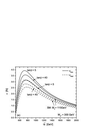
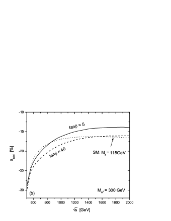
Figure 4: The Born and the full one-loop level electroweak corrected cross sections(shown in Fig.4(a)) as well as the corresponding relative corrections $\delta_{total}$(shown in Fig.4(b)) for the process $e^{+}e^{-}\to t\bar{t}h^{0}$ as the functions of the c.m.s energy $\sqrt{s}$.

By taking the MSSM parameters as $M_{SUSY}=300~{}{\rm GeV}$, $M_{2}=200~{}{\rm GeV}$, $\mu=200~{}{\rm GeV}$, $A_{f}=200~{}{\rm GeV}$ and $M_{A^{0}}=300~{}{\rm GeV}$, we present Fig.4(a) to show the Born cross section $\sigma_{tree}$ and the full ${\cal O}(\alpha_{ew})$ corrected cross section $\sigma_{total}$ as the functions of the c.m.s. energy $\sqrt{s}$ in the SM with $m_{h}=115~{}{\rm GeV}$, and in the MSSM with $\tan\beta=5$ and $\tan\beta=40$, which correspond to $m_{h^{0}}=98.36~{}{\rm GeV}$ for $\tan\beta=5$ and $m_{h^{0}}=105.87~{}{\rm GeV}$ for $\tan\beta=40$, respectively. We also take the same input parameters as in Refs.[15, 16], and get the coincident results for the SM with the corresponding ones in these references. That comparison is a check for the correctness of our calculation. In the figure the c.m.s. energy $\sqrt{s}$ varies from $500~{}{\rm GeV}$ to $2000~{}{\rm GeV}$. It shows that each curve has a peak in the region around the c.m.s. colliding energy $\sqrt{s}\sim 700~{}{\rm GeV}$ due to the phase space feature, and all the curves decrease gently after reaching their maximal values. We can read out from the figure that the $\sigma_{tree}$ can reach their own maximum values of $3.96~{}{\rm fb}$ and $3.59~{}{\rm fb}$ at $\sqrt{s}\sim 700~{}{\rm GeV}$ for $\tan\beta=5$ and $\tan\beta=40$, respectively, but their maximum values are shifted to $3.17~{}{\rm fb}$ and $2.84~{}{\rm fb}$ after including the supersymmetric electroweak radiative corrections. Fig.4(b) shows the dependence of the full ${\cal O}(\alpha_{ew})$ relative correction $\delta_{total}$ on the c.m.s energy $\sqrt{s}$. There the relative correction increases rapidly with the increment of the c.m.s. energy in the vicinity of the threshold energy, but is insensitive to c.m.s. colliding energy when $\sqrt{s}\gtrsim 1200~{}{\rm GeV}$. We present some exact numerical results of $\sigma_{tree}$, $\sigma_{total}$ and $\delta_{total}$ in Table 1 by taking above input parameters.

$\sqrt{{s}}~{}[{\rm GeV}]$	$tan\beta$	$M_{h^{0}}[{\rm GeV}]$	$\sigma_{tree}[{\rm fb}]$	$\sigma_{total}[{\rm fb}]$	$\delta_{total}[\%]$
500	5	98.36	1.070746(1)	0.761(1)	-28.97(9)
	40	105.87	0.7086974(7)	0.4938(6)	-30.33(8)
800	5	98.36	3.808457(3)	3.105(5)	-18.5(1)
	40	105.87	3.515246(3)	2.800(4)	-20.4(1)
1000	5	98.36	3.065664(3)	2.568(4)	-16.2(1)
	40	105.87	2.889250(3)	2.362(4)	-18.2(1)
2000	5	98.36	1.073347(1)	0.924(2)	-13.9(2)
	40	105.87	1.041033(1)	0.874(2)	-16.1(2)

Table 1: Taking $M_{A^{0}}=300~{}GeV$, the Born cross section $\sigma_{tree}$ and the corrected cross section $\sigma_{total}$ as well as the corresponding relative corrections $\delta_{total}$ for different values of $\tan\beta$ and c.m.s. energy $\sqrt{s}$.

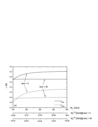
Figure 5: The cross sections at the Born and the one-loop electroweak levels, and their corresponding relative corrections for the process $e^{+}e^{-}\to t\bar{t}h^{0}$ as the functions of $M_{A^{0}}(m_{h^{0}})$ with $\sqrt{s}=800~{}GeV$ and $\tan\beta=5,~{}40$, are shown in Fig.5(a) and Fig.5(b), respectively.

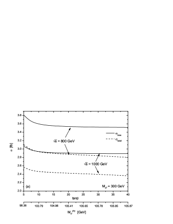
Figure 6: The Born and the one-loop level electroweak corrected cross sections(shown in Fig.6(a)) as well as the corresponding relative corrections(shown in Fig.6(b)) for the process $e^{+}e^{-}\to t\bar{t}h^{0}$ as the functions of $\tan\beta$ with $\sqrt{s}=800~{}GeV$ and $\sqrt{s}=1000~{}GeV$ separately.

In Fig.5(a) we present the Born cross section $\sigma_{tree}$ and the full one-loop electroweak corrected cross section $\sigma_{total}$ for the process $e^{+}e^{-}\to t\bar{t}h^{0}$ as the functions of the mass of the CP-odd Higgs boson $A^{0}$(or $m_{h^{0}}$) on the conditions of $M_{SUSY}=300~{}{\rm GeV}$, $M_{2}=200~{}{\rm GeV}$, $\mu=200~{}{\rm GeV}$, $\sqrt{s}=800~{}GeV$ and $A_{f}=200~{}{\rm GeV}$, for $\tan\beta=5$ and $\tan\beta=40$ respectively. The corresponding relative corrections are depicted in Fig.5(b). As shown in these two figures all the curves of $\sigma_{tree}$, $\sigma_{total}$ and relative correction $\delta$, for both $\tan\beta=5$ and $\tan\beta=40$, are less sensitive to $M_{A^{0}}(m_{h^{0}})$, except the relative correction for $\tan\beta=5$ in the region of $M_{A^{0}}<250~{}GeV$. The behavior for that is due to the fact that when $M_{A^{0}}$ goes from $150~{}GeV$ to $350~{}GeV$, the phase space of this process does not change significantly(especially for $\tan\beta=40$), since the physical mass of $h^{0}$ varies in a small range from $94.69~{}GeV(105.76~{}GeV)$ to $98.6~{}GeV(105.89~{}GeV)$ for $\tan\beta=5(\tan\beta=40)$ as shown in Fig.5(a) and Fig.5(b).

The Born cross section and the one-loop electroweak corrected cross section as the functions of $\tan\beta$ are depicted in Fig.6(a) on the conditions of $M_{A^{0}}=300~{}{\rm GeV}$, $M_{SUSY}=300~{}{\rm GeV}$, $M_{2}=200~{}{\rm GeV}$, $\mu=200~{}{\rm GeV}$ and $A_{f}=200~{}{\rm GeV}$. In this figure both $\sigma_{tree}$ curves for $\sqrt{s}=800~{}{\rm GeV}$ and $\sqrt{s}=1000~{}{\rm GeV}$ decrease slowly with the increment of $\tan\beta$ except in the region of $\tan\beta<10$. To clarify the dependence of the electroweak relative correction corresponding to Fig.6(a) on $\tan\beta$, we plot the relative correction versus $\tan\beta$ in Fig.6(b). One can read from Fig.6(b) that the relative corrections are again negative as shown in Fig.5, and decrease obviously as $\tan\beta$ increasing from $10$ to $40$. The values vary from about $-18.4\%$ to $-20.4\%$ for $\sqrt{s}=800~{}{\rm GeV}$, and from $-16.2\%$ to $-18.2\%$ for $\sqrt{s}=1000~{}{\rm GeV}$ as $\tan\beta$ running from $5$ to $40$.

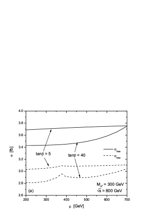
Figure 7: The Born and the one-loop level electroweak corrected cross sections(shown in Fig.7(a)) as well as the corresponding relative corrections(shown in Fig.7(b)) for the process $e^{+}e^{-}\to t\bar{t}h^{0}$ as the functions of the $\mu$ by taking $\tan\beta=5$ and $\tan\beta=40$ separately.

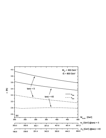
Figure 8: The Born and the one-loop level electroweak corrected cross sections(shown in Fig.8(a)) as well as the corresponding relative corrections(shown in Fig.8(b)) for the process $e^{+}e^{-}\to t\bar{t}h^{0}$ as the functions of the $M_{SUSY}(m_{\tilde{t}_{1}})$ by taking $\tan\beta=5$ and $\tan\beta=40$ separately. The Higgs mass $m_{h^{0}}$ involving up to two-loop level radiative corrections as the functions of $M_{SUSY}$ are plotted in Fig.8(c).

In Fig.7(a) we present the Born cross section $\sigma_{tree}$ and the full ${\cal O}(\alpha_{ew})$ electroweak corrected cross section $\sigma_{total}$ as the functions of Higgsino-mass parameter $\mu$ with the conditions of $\sqrt{s}=800~{}{\rm GeV}$, $M_{A^{0}}=300~{}{\rm GeV}$, $M_{SUSY}=400~{}{\rm GeV}$, $M_{2}=200~{}{\rm GeV}$ and $A_{f}=200~{}{\rm GeV}$. The two full-line curves and two dashed-line curves in the figure are corresponding to $\tan\beta=5$ and $\tan\beta=40$ separately. As shown in Fig.7(a), each curve of $\sigma_{total}$ has a small spike which shows the resonance effect in the vicinity of $\sqrt{s}\simeq 2m_{\tilde{\chi}_{2}^{+}}$. For $\tan\beta=5$, both $\sigma_{tree}$ and $\sigma_{total}$ are less sensitive to $\mu$, while for $\tan\beta=40$, the Born and the electroweak corrected cross sections increase smoothly with the increment of $\mu$ except in the range around the resonance peak on the dashed curve for $\sigma_{total}$. With the same parameter conditions, the dependence of relative correction on $\mu$ is displayed in Fig.7(b). For $\tan\beta=5$, the relative correction is also less sensitive to $\mu$ except in the vicinity of $\mu\sim 377.3~{}{\rm GeV}$ for the resonance effect. But the $\delta_{total}$ curve for $\tan\beta=40$ has a more obvious resonance peak in the vicinity of $\mu\sim 377.3~{}{\rm GeV}$, and after arriving the peak value it decreases rapidly with the increment of $\mu$.

We present the dependence of the Born cross section and the corrected cross section on the sfermion sector parameter $M_{SUSY}$(or $m_{\tilde{t}_{1}}$) in Fig.8(a), on the conditions of $\sqrt{s}=800~{}{\rm GeV}$, $M_{A^{0}}=300~{}{\rm GeV}$, $\mu=200~{}{\rm GeV}$, $M_{2}=200~{}{\rm GeV}$ and $A_{f}=200~{}{\rm GeV}$, with $\tan\beta=5$ and $\tan\beta=40$ respectively. From this figure we find that both Born cross sections and the electroweak corrected cross sections decrease slowly with the increment of $M_{SUSY}$ in the range of $200~{}{\rm GeV}<M_{SUSY}<500~{}{\rm GeV}$, since we take the radiative corrected Higgs mass $m_{h^{0}}$ involving two-loop corrections as its physical mass. The relations between the physical Higgs mass $m_{h^{0}}$ and the soft-SUSY- breaking mass parameter $M_{SUSY}$ are depicted in Fig.8(c). We can see from Fig.8(a) and Fig.8(c) that the dependence of the Born cross-section on $M_{SUSY}$ is due to the Higgs boson mass $m_{h^{0}}$ being related to $M_{SUSY}$ at loop level. The relative corrections as the functions of $M_{SUSY}$ corresponding to Fig.8(a) are depicted in Fig.8(b). In contrast to the case of $\tan\beta=5$, the full ${\cal O}(\alpha_{ew})$ electroweak relative correction for $\tan\beta=40$ is more sensitive to parameter $M_{SUSY}$. The electroweak relative correction for $\tan\beta=40$ varies in the range between $-22.6\%$ and $-16.9\%$ when $M_{SUSY}$ goes from $200~{}GeV$ to $500~{}GeV$.

Figure 9: The electroweak relative corrections for the process $e^{+}e^{-}\to t\bar{t}h^{0}$ as the functions of the $M_{2}$ with $\tan\beta=5$ and $\tan\beta=40$, respectively.

Figure 10: The electroweak relative corrections for the process $e^{+}e^{-}\to t\bar{t}h^{0}$ as the functions of the $A_{f}$ with $\tan\beta=5$ and $\tan\beta=40$, respectively.

In Fig.9 and Fig.10, we depict the dependence of the full ${\cal O}(\alpha_{ew})$ electroweak relative correction on the gaugino mass parameter $M_{2}$ (or neutralino mass $m_{\tilde{\chi}^{0}_{1}}$) and the soft trilinear couplings for sfermions $A_{f}$ (or scalar top-quark mass $m_{\tilde{t}_{1}}$) respectively. There we take the input parameters as $\sqrt{s}=800~{}{\rm GeV}$, $M_{A^{0}}=300~{}{\rm GeV}$, $\mu=200~{}{\rm GeV}$, $M_{SUSY}=200~{}{\rm GeV}$ and $A_{f}=200~{}{\rm GeV}$ for Fig.9 and $\sqrt{s}=800~{}{\rm GeV}$, $M_{A^{0}}=300~{}{\rm GeV}$, $\mu=200~{}{\rm GeV}$, $M_{SUSY}=200~{}{\rm GeV}$ and $M_{2}=200~{}{\rm GeV}$ for Fig.10. In Fig.9, each curve has a small peak at about $M_{2}\sim 370~{}GeV$. That reflects the resonance effect satisfying the condition of $\sqrt{s}\sim 2m_{\tilde{\chi}_{2}^{+}}$. From these two figures we can see that the one-loop electroweak relative correction are less sensitive to $M_{2}$(or $m_{\tilde{\chi}^{0}_{1}}$) and $A_{f}$(or $m_{\tilde{t}_{1}}$) quantitatively. The variation ranges of the relative corrections for both curves in Fig.9 are less than $1\%$ in our chosen parameter space. Fig.10 shows that the variations of the relative corrections for curves of $\tan\beta=40$ and $\tan\beta=5$ are less than $1\%$ and $3\%$ respectively, when $A_{f}$ goes from $100~{}GeV$ to $350~{}GeV$.

4 Summary

In this paper, we present the calculation of the full ${\cal O}(\alpha_{ew})$ electroweak correction to the process $e^{+}e^{-}\to t\bar{t}h^{0}$ at a LC in the MSSM. We analyze the numerical results and investigate the dependence of the cross section and relative correction on $\sqrt{s}$ and several MSSM parameters. We find that these corrections generally reduce the Born cross sections and the relative correction is typically of order $-20\%$. The electroweak relative correction is strongly related to $\tan\beta$, and has obvious dependence on $M_{A^{0}}$ and $M_{SUSY}$ on the conditions of $\tan\beta=5$ and $\tan\beta=40$, respectively. The results also show that the one-loop electroweak relative correction is generally less sensitive to $M_{2}$ and $A_{f}$ in the range of $150~{}{\rm GeV}<M_{2}<500~{}{\rm GeV}$ and $100~{}{\rm GeV}<A_{f}<350~{}{\rm GeV}$, respectively. We conclude that the complete ${\cal O}(\alpha_{ew})$ electroweak corrections to the process $e^{+}e^{-}\to t\bar{t}h^{0}$ are generally significant and cannot be neglected in the precise experiment analysis.

Acknowledgement:

This work was supported in part by the National Natural Science Foundation of China and a special fund sponsored by China Academy of Science.

References

- [1] S. L. Glashow, Nucl. Phys. B22, 579 (1961) ; S. Weinberg, Phys. Rev. Lett. 19, 1264 (1967); A. Salam, in Proceedings of the 8th Nobel Symposium, Stockholm, 1968, edited by N. Svartholm (Almquist and Wiksells, Stockholm, 1968), p.367; H. D. Politzer, Phys. Rep. 14 129 (1974).
- [2] P. W. Higgs, Phys. Lett 12, 132 (1964), Phys. Rev. Lett. 13, 508 (1964); Phys. Rev. 145, 1156 (1966); F. Englert and R. Brout, Phys. Rev. Lett. 13, 321 (1964); G. S. Guralnik, C. R. Hagen, and T. W. B. Kibble, ibid. 13, 585 (1964); T. W. B. Kibble, Phys. Rev. 155, 1554 (1967).
- [3] (ALEPH), (DELPHI), (L3) and (POAL) Collaborations, the LEP working group for Higgs boson searches’LHWG Note 2002-01 (2002), in ICHEP’02 Amsterdam, 2002; and additional updates at http://lephiggs.web.cern.ch/LEPHIGGS/www/Welcome.html; P. A. McNamara and S. L. Wu, Rept. Prog. Phys. 65, 465 (2002).
- [4] The LEP Collaborations: ALEPH Collaboration, DELPHI Collaboration, L3 Collaboration, OPAL Collaboration, the LEP Electroweak Working Group, the SLD Electroweak, Heavy Flavour Groups, CERN-PH-EP/2004-069, LEPEWWG/2004-01, arXiv:hep-ex/0412015.
- [5] (ALEPH), (DELPHI), (L3) and (POAL) Collaborations, the LEP working group for Higgs boson searches’LHWG Note 2002-04, LHWG Note 2002-05.
- [6] The LEP Collaborations: ALEPH Collaboration, DELPHI Collaboration, L3 Collaboration, OPAL Collaboration, the LEP Electroweak Working Group, the SLD Heavy Flavour Working Group, LEPEWWG/2002-02, CERN-EP/2002-091, hep-ex/0212036; S. Alekhin et.al., ’The QCD/SM Working Group: Summary Report’, arXiv:hep-ph/0204316.
- [7] ’TESLA: The superconducting electron positron linear collider with an integrated X-ray laser laboratory. Technical design report, Part 2: The Accelerator’, Report No. DESY-01-11, edited by R. Brinkmann, K. Flottmann, J. Rossbach, P. Schmuser, N. Walker, and H. Weise, 2001 (unpublished).
- [8] C. Adolphsen et al., (International Study Group Collaboration), ’International study group progress report on linear collider development’,Report Nos. SLAC-R-559 and KEK-REPORT-2000-7, 2000 (unpubplished).
- [9] N. Akasaka et al., ’JLC design study’, Report No. KEK-REPORT-97-1.
- [10] ’A 3 TeV Linear Collider Based on CLIC Technology’,Report No. CERN-2000-008, edited by G. Guignard (unpublished).
- [11] L. Reina and S. Dawson, Phys. Rev. Lett. 87, 201804 (2001).
- [12] L. Reina, S. Dawson and D. Wackeroth, Phys. Rev. D65, 053017 (2002).
- [13] W. Beenakker, S. Dittmaier, M. Krämer, B. Plumper, M. Spira and P. M. Zerwas, Phys. Rev. Lett. 87, 201805 (2001); Nucl. Phys. B653, 151 (2003).
- [14] D. Rainwater, M. Spira and D. Zeppenfeld, Report No. MAD-PH-02-1260 (unpublished)..
- [15] Y. You, W.-G. Ma, H. Chen, R.-Y. Zhang, Y.-B. Sun, H.-S. Hou, Phys. Lett. B571 (2003) 85, arXiv:hep-ph/0306036; G. Belanger, F. Boudjema, J. Fujimoto, T. Ishikawa, T. Kaneko, K. Kato, Y. Shimizu and Y. Yasui, Phys. Lett. B571 (2003)163, arXiv:hep-ph/0307029; A. Denner, S. Dittmaier, M. Roth, M. M. Weber, Phys. Lett. B575 (2003)290, arXiv:hep-ph/0307193.
- [16] A. Denner, S. Dittmaier, M. Roth and M. M. Weber, Nucl.Phys. B680 85 (2004); Eur. Phys. J. C33 S635 (2004); C. Farrell, A. H. Hoang, Phys. Rev. D72 (2005) 014007, arXiv:hep-ph/0504220.
- [17] X. H. Wu, C. S. Li and J. J. Liu, arXiv:hep-ph/0308012.
- [18] S. H. Zhu, arXiv:hep-ph/0212273.
- [19] P. Häfliger and M. Spira, arXiv:hep-ph/0501164.
- [20] K. Cheung, Phys. Rev. D47 (1993) 3750.
- [21] H. Chen, W.-G. Ma, R.-Y. Zhang, P.-J. Zhou, H.-S. Hou and Y.-B. Sun, Nucl. Phys. B683 196 (2004).
- [22] G. Passarino and M. Veltman, Nucl. Phys. B160 151 (1979).
- [23] T. Hahn, Comp. Phys. Commun. 140 418 (2001).
- [24] J. A. M. Vermaseren, arXiv:math-ph/0010025.
- [25] A. Denner and S. Dittmaier, Nucl. Phys. B658 175 (2003).
- [26] S. Eidelman, et al., Phys. Lett. B592 1 (2004).
- [27] J. Guasch, W. Hollik, J. Sola, J. High Energy Phys. 10 (2002) 040, arXiv:hep-ph/0207364; W. Hollik, E. Kraus, M. Roth, C. Rupp, K. Sibold and D. Stoecklinger, Nucl.Phys. B639 (2002) 3-65, arXiv:hep-ph/0204350.
- [28] D. Pierce and A. Papadopoulos, Phys. Rev. D47 222 (1993); R.-Y. Zhang, W.-G. Ma, L.-H. Wan and Y. Jiang, Phys. Rev. D65 (2002)075018.
- [29] B.W. Harris and J.F. Owens, Phys. Rev. D 65 (2002) 094032
- [30] G. ’t Hooft and M. Veltman, Nucl. Phys. B153 365 (1979).
- [31] T. Ishikawa, T. Kaneko, K. Kato, S. Kawabata, Y. Shimizu and H. Tanaka, ”GRACE manual”, KEK report 92-19, 1993(unpublished)..
- [32] F. Jegerlehner, Report No. DESY 01-029 (unpublished).
- [33] C. Weber, H. Eberl, W. Majerotto, Phys. Lett. B572 56 (2003).
- [34] H. Eberl, M. Kincel, W. Majerotto and Y. Yamada, Nucl. Phys. B625 372 (2002).
- [35] K. Kovařík, C. Weber, H. Eberl, W. Majerotto, Phys. Lett. B591 242 (2004).
- [36] Thomas Hahn and Christian Schappacher, Comput. Phys. Commun. 143 54 (2002).
- [37] S. Heinemeyer, W. Hollik, G. Weiglein, Phys.Lett. B455, 179 (1999).
- [38] A. Freitas, A. van Manteuffel and P.M. Zerwas, Eur.Phys.J. C40 435 (2005), arXiv:hep-ph/0408341.
- [39] J. F. Gunion, H. E. Haber, Nucl. Phys. B272 1 (1986) .