First Order QED Corrections to the Parity-Violating Asymmetry in Møller Scattering

Abstract

We compute a full set of the first order QED corrections to the parity-violating observables in polarized Møller scattering. We employ a covariant method of removing infrared divergences, computing corrections without introducing any unphysical parameters. When applied to the kinematics of the SLAC E158 experiment, the QED corrections reduce the parity violating asymmetry by $4.5\%$. We combine our results with the previous calculations of the first-order electroweak corrections and obtain the complete $\mathcal{(}O)(\alpha)$ prescription for relating the experimental asymmetry $A_{LR}$ to the low-energy value of the weak mixing angle $\sin^{2}\theta_{W}$. Our results are applicable to the recent measurement of $A_{LR}$ by the SLAC E158 collaboration, as well as to the future parity violation experiments.

I Introduction

Measurements of the parity-violating observables in electron scattering provide information about low-energy structure of weak neutral current processes. Such observables arise from the interference between the weak and electromagnetic amplitudes ref:Zeldovich , and are sensitive to the electroweak couplings. In the Standard Model, the couplings of the $Z^{0}$ boson to the fermions are determined by the weak mixing angle $\theta_{\rm W}$, which has been measured with high precision at the $Z^{0}$ resonance ref:PDG2004 . Precision measurements of the low-energy parity-violating observables provide an independent determination of the weak mixing angle, directly test higher order electroweak corrections, and provide strong independent constraints on the new physics contributions at the TeV scales ref:MarcianoRosner .

The experiment E158 at the Stanford Linear Accelerator Center (SLAC) has measured the parity-violating left-right asymmetry $A_{LR}$ in Møller scattering of polarized 50 GeV electrons off unpolarized atomic electrons in a liquid hydrogen target ref:E158 . The final uncertainty on $A_{LR}$ is about 10%. The measurement of $A_{LR}$ translates into the measurement of $\sin^{2}\theta_{W}$ with a precision of $\sigma(\sin^{2}\theta_{W})\approx 0.001$ at low momentum transfer $Q^{2}\approx 0.03~{}{\rm GeV}^{2}/c^{2}$, and is sensitive to both electroweak one-loop radiative corrections and new physics phenomena at the TeV scales.

A precise comparison of the experimental results with the Standard Model predictions requires detailed understanding of the radiative corrections, including effects of the QED bremsstrahlung. The leading-order electroweak corrections to the Møller scattering have been computed a number of years ago cz-marc ; denn . The authors of Ref. cz-marc factorized out the soft bremsstrahlung contribution, but did not include the effects of hard bremsstrahlung, arguing that their effects are small, and would require the knowledge of experimental kinematics and acceptance. In this paper, improving on the calculation of Ref. zyk , we present a complete calculation of the first order QED corrections. The detailed analysis shows that the QED corrections are indeed small but not insignificant, compared to the systematic uncertainties of E158 and the projected uncertainties of the future parity violation experiments.

Experimentally, Møller scattering is often used to measure polarization of electron beams ref:polarimetry . In such measurements, both beam and target electrons are polarized, and electroweak effects can typically be neglected. QED corrections to the parity-conserving polarized Møller scattering have been computed in Ref. suarez ; IlyichevZykunov and are relatively important, compared to the typical precision of Møller polarimeters. Similar to Ref. suarez ; IlyichevZykunov , we perform our calculations in the covariant framework of Bardin and Shumeiko covar , which allows us to cancel out infrared divergences without introducing unphysical parameters (such as a frame-dependent cutoff $\Delta E$ that separates the soft bremsstrahlung region from the hard bremsstrahlung contributions).

This paper is organized as follows. Section II introduces the kinematics of the Møller scattering and Born cross section and parity-violating asymmetry. Section III explains the regularization of infrared divergences. Section VI presents numerical results applied to the kinematics of SLAC E158 experiment.

II Definitions, Born Cross Section, and Kinematics

The lowest-order (Born) cross section for Møller scattering, defined by the Feynman diagrams in Fig. 1, can be written as

$$\sigma^{0}=\frac{2\pi\alpha^{2}}{s}\sum_{i,j=\gamma,Z}[\lambda_{-}^{ij}(u^{2}D^{i}(t)D^{j}(t)+t^{2}D^{i}(u)D^{j}(u))+\lambda_{+}^{ij}s^{2}(D^{i}(t)+D^{i}(t))(D^{j}(t)+D^{j}(u))],$$ (1)

where the four-momenta of the initial and final electrons $k_{1},\;p_{1}$ and $k_{2},\;p_{2}$ (see Fig.1) are combined to form Mandelstam invariants

$$s=(k_{1}+p_{1})^{2},\ t=(k_{1}-k_{2})^{2},\ u=(k_{2}-p_{1})^{2}\ .$$ (2)

In Eq. (1) and hereafter, we use a short-hand notation $\sigma\equiv d\sigma/dy$.

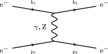
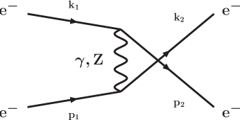
Figure 1: Born-level diagrams for Møller scattering: $t$-channel (left) and $u$-channel (right).

The Born cross section in Eq. (1) is written in terms of the photon and $Z^{0}$ propagators

$$D^{i}(k)\equiv D^{ik}=\frac{1}{k-m_{i}^{2}}\ (i=\gamma,Z)$$ (3)

and the coupling factors

$$\lambda_{\pm}^{ij}={\lambda_{1}}_{B}^{ij}{\lambda_{1}}_{T}^{ij}\pm{\lambda_{2}}_{B}^{ij}{\lambda_{2}}_{T}^{ij}\ .$$ (4)

The latter in turn depend on the polarizations of the beam ($p_{B}$) and target ($p_{T}$) electrons:

$${\lambda_{1}}_{B(T)}^{ij}=\lambda_{V}^{ij}-p_{B(T)}\lambda_{A}^{ij}\ ,\ {\lambda_{2}}_{B(T)}^{ij}=\lambda_{A}^{ij}-p_{B(T)}\lambda_{V}^{ij},$$ (5)

$$\lambda_{V}^{ij}=v^{i}v^{j}+a^{i}a^{j},\ \lambda_{A}^{ij}=v^{i}a^{j}+a^{i}v^{j},$$ (6)

where $v^{i},\ a^{i}$ are the vector and axial-vector coupling constants for the photon and $Z^{0}$:

$$v^{\gamma}=1,\ a^{\gamma}=0,$$ (7)

$$v^{Z} = (-1+4s_{W}^{2})/(4s_{W}c_{W})$$

$$a^{Z} = -1/(4s_{W}c_{W})$$ (8)

and $s_{W}$ ($c_{W}$) is sine (cosine) of the Weinberg angle.

It is convenient to rewrite the cross section in terms of four Born-level matrix elements $M^{0}_{l}$:

$$\sigma^{0}=\frac{\pi\alpha^{2}}{s}\mathrm{Re}\sum_{l=1}^{4}(M^{0}_{l}+{\hat{M}}^{0}_{l}),$$ (9)

where matrix elements $\hat{M}^{0}_{l}$ are obtained from $M^{0}_{l}$ by crossing symmetry $t\leftrightarrow u$. The matrix elements $M^{0}_{l}$ are expressed through the “even” and “odd” functions $M_{e}$ and $M_{o}$:

$$\displaystyle M^{0}_{1} = D^{\gamma t}(D^{\gamma t}M_{e}^{\gamma\gamma\gamma\gamma}-D^{\gamma u}M_{o}^{\gamma\gamma\gamma\gamma}),\$$

$$M^{0}_{2} = D^{\gamma t}(D^{Zt}M_{e}^{\gamma Z\gamma Z}-D^{Zu}M_{o}^{\gamma Z\gamma Z}),\$$

$$M^{0}_{3} = D^{Zt}(D^{\gamma t}M_{e}^{Z\gamma Z\gamma}-D^{\gamma u}M_{o}^{Z\gamma Z\gamma}),\$$

$$M^{0}_{4} = D^{Zt}(D^{Zt}M_{e}^{ZZZZ}-D^{Zu}M_{o}^{ZZZZ})\ .$$ (10)

The matrix elements $M_{e}$ and $M_{o}$ are defined in such a way that they can be used, with minimal modifications, in both Born and first-order matrix elements. They are defined in terms of the couplings $\lambda$

$$M^{ijkl}_{e} = 2(s^{2}+u^{2}){\lambda_{1}}_{B}^{ij}{\lambda_{1}}_{T}^{kl}+2(s^{2}-u^{2}){\lambda_{2}}_{B}^{ij}{\lambda_{2}}_{T}^{kl},$$ (11)

$$M^{ijkl}_{o} = -2s^{2}({\lambda_{1}}_{B}^{ij}{\lambda_{1}}_{T}^{kl}+{\lambda_{2}}_{B}^{ij}{\lambda_{2}}_{T}^{kl})\ .$$ (12)

The kinematic variable $y$ is defined as

$$y=-\frac{t}{s}\approx\frac{1-\cos\Theta}{2}\frac{E^{*^{\prime}}}{E^{*}},$$ (13)

where $\Theta$ is the center of mass (CMS) scattering angle of the detected electron with momentum $k_{2}$. $E^{*}(E^{*^{\prime}})$ is the energy of the initial (detected) electron in CMS, respectively. In the Born approximation, the Møller scattering is elastic and $E^{*}=E^{*^{\prime}}$, therefore

$$y_{\rm Born}=\frac{1-\cos\Theta}{2}=1-\frac{E^{{}^{\prime}}}{E}\$$ (14)

where $E$ and $E^{{}^{\prime}}$ are the initial and scattered electron energies in the Lab frame, respectively. Whenever possible, we ignore the electron mass $m$ (which cannot be done in the collinear singularity regions).

At the Born level, the unpolarized (averaged over helicity states) cross section is given analytically by Moller

$$\sigma^{0}=\frac{2\pi\alpha^{2}}{sy^{2}(1-y)^{2}}\left(1+y^{4}+(1-y)^{4}\right)\,.$$ (15)

Polarization asymmetry $A_{LR}$ is conventionally defined as

$$A_{LR}\equiv\frac{\sigma_{LL}+\sigma_{LR}-\sigma_{RL}-\sigma_{RR}}{\sigma_{LL}+\sigma_{LR}+\sigma_{RL}+\sigma_{RR}}\ ,$$ (16)

where the first helicity index refers to the beam electrons, and the second helicity index corresponds to the target electrons. Since the target helicity is summed over, $A_{LR}$ defined by Eq. (16) is a parity-violating observable. The Born-level asymmetry is given by cz-marc

$$A_{LR}^{0} = \mathcal{A}^{0}(Q^{2},y)\left(1-4\sin^{2}\theta_{W}\right)=\frac{G_{F}s}{\sqrt{2}\pi\alpha}\frac{y(1-y)}{1+y^{4}+(1-y)^{4}}\left(1-4\sin^{2}\theta_{W}\right)\,,$$ (17)

where $\mathcal{A}^{0}(Q^{2},y)$ is an experimental acceptance-dependent analyzing power. Kinematics of the E158 experiment correspond to the laboratory beam energies of $E=45(48)$ GeV and CMS scattering angles $-0.5<\cos\Theta\leq 0$, or average invariants $s=2mE\approx 0.048~{}{\rm GeV}^{2}/c^{2}$, $Q^{2}=-t=0.026~{}{\rm GeV}^{2}/c^{2}$ and $y\approx 0.6$ ref:E158 .

We perform our calculation in the on-shell (OS) renormalization scheme, defining the weak mixing angle to all orders in perturbation theory as $c_{W}\equiv m_{W}/m_{Z}$, where $m_{W}$ and $m_{Z}$ are the physical masses of the $W^{\pm}$ and $Z^{0}$ bosons, respectively. For consistency with the precision electroweak measurements ref:PDG2004 ; ref:EWWG , we use

$$m_{W} = 80.390~{}{\rm GeV}$$ (18)

$$m_{Z} = 91.188~{}{\rm GeV}$$ (19)

which implies

$$\sin^{2}\theta_{W}=0.2228$$ (20)

in the on-shell scheme. As we will note in Section VI, while the absolute value of the Born asymmetry depends on the electron neutral current coupling $1-4\sin^{2}\theta_{W}$, the relative corrections to the experimentally measured asymmetries computed here are quite insensitive to the choice of couplings or the renormalization scheme.

III Radiative Corrections

It is well known that effects of “internal” bremsstrahlung (real photon emission) need to be combined with the contributions from the other one-loop (leading order) electroweak radiative corrections (so-called virtual, or V-contributions). The virtual contributions to Møller scattering have been studied extensively cz-marc ; denn and are not repeated here. However, we need the infrared-divergent part of the V-contributions, which cancels out the corresponding divergences in the bremsstrahlung cross section. Naturally, the extraction of the IR-divergent parts is a somewhat subjective procedure, which may lead to ambiguities similar to the concept of scheme dependence in the ultraviolet renormalization. We follow the framework of Bardin and Shumeiko covar and extract the infrared-divergent contributions that are strictly proportional to the Born cross section. Such contributions cancel in the parity-violating asymmetry, and remain small even after other corrections are taken into account. We take the infrared-divergent parts of the virtual corrections from BSH86 ; Hol90 , which include the vacuum polarization and vertex correction contributions. We also compute the IR-divergent $\gamma\gamma$ and $\gamma Z$ box diagrams.

The virtual contributions to the Møller scattering cross section and asymmetry can be classified into three categories: the vacuum polarizations of the gauge boson propagators, vertex corrections, and box diagrams (see Fig. 2):

$$\sigma^{V}=\sigma^{S}+\sigma^{Ver}+\sigma^{B}\ .$$ (21)

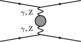
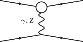
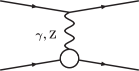
(a)	(b)	(c)
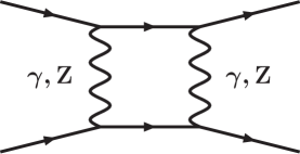
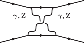
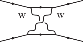
(d)	(e)	(f)

Figure 2: One-loop $t$-channel contributions to Møller scattering. Circles represent vacuum polarization (a) and vertex correction contributions (b,c), given in BSH86 ; Hol90 .

The vacuum polarizations of $\gamma$ and $Z^{0}$ bosons are infrared-convergent, and are not considered in this paper. The infrared-divergent parts of the vertex corrections (Figures 2b and 2c) are obtained from form-factors $\delta F_{V,A}^{je}$ given in BSH86 (for $k^{2}=t,u$). Substituting the coupling constants for the vertex form-factors (e.g. $v^{\gamma}\rightarrow\delta F_{V}^{\gamma e}$) in the expressions for the Born functions $M_{e,o}$, we get the vertex part of the cross section

$$\sigma^{Ver}=\frac{2\pi\alpha^{2}}{s}\mathrm{Re}\sum_{l=1}^{4}(M^{V}_{l}+{\hat{M}}^{V}_{l}),$$ (22)

where

$$\displaystyle M^{V}_{1} = D^{\gamma t}(D^{\gamma t}(M_{e}^{F^{\gamma}\gamma\gamma\gamma}+M_{e}^{\gamma\gamma F^{\gamma}\gamma})-D^{\gamma u}(M_{o}^{F^{\gamma}\gamma\gamma\gamma}+M_{o}^{\gamma\gamma F^{\gamma}\gamma})),$$

$$M^{V}_{2} = D^{\gamma t}(D^{Zt}(M_{e}^{F^{\gamma}Z\gamma Z}+M_{e}^{\gamma ZF^{\gamma}Z})-D^{Zu}(M_{o}^{F^{\gamma}Z\gamma Z}+M_{o}^{\gamma ZF^{\gamma}Z})),$$

$$M^{V}_{3} = D^{Zt}(D^{\gamma t}(M_{e}^{F^{Z}\gamma Z\gamma}+M_{e}^{Z\gamma F^{Z}\gamma})-D^{\gamma u}(M_{o}^{F^{Z}\gamma Z\gamma}+M_{o}^{Z\gamma F^{Z}\gamma})),$$

$$M^{V}_{4} = D^{Zt}(D^{Zt}(M_{e}^{F^{Z}ZZZ}+M_{e}^{ZZF^{Z}Z})-D^{Zu}(M_{o}^{F^{Z}ZZZ}+M_{o}^{ZZF^{Z}Z})).$$ (23)

The box diagrams with at least one photon (i.e. Figures 2d and 2e plus $u$-channel graphs) also contain infrared divergences. The diagrams with two $Z^{0}$ or two $W$ bosons are infrared-convergent and are not considered here. We compute the box diagram contribution as a sum of the infrared-divergent and infrared-finite parts $\sigma^{B}=\sigma^{B}_{F}+\sigma^{B}_{IR}$. The IR-finite parts of the $\gamma\gamma$ and $\gamma Z$ boxes are expressed by

$$\sigma^{B}_{F}=-\frac{2\alpha^{3}}{s}\sum_{k=\gamma,Z}\left(B_{\gamma\gamma}^{k}+B_{\gamma Z}^{k}\right)+\bigl{(}t\leftrightarrow u\bigr{)}\ .$$ (24)

The terms $B$ have the following form:

$$B_{(\gamma\gamma)}^{k} = D^{kt}\lambda_{-}^{\gamma k}\delta^{1}_{(\gamma\gamma)}+(D^{kt}+D^{ku})\lambda_{+}^{\gamma k}\delta^{2}_{(\gamma\gamma)}$$

$$B_{(\gamma Z)}^{k} = D^{kt}\lambda_{-}^{Zk}\delta^{1}_{(\gamma Z)}+(D^{kt}+D^{ku})\lambda_{+}^{Zk}\delta^{2}_{(\gamma Z)}$$ (25)

At low energies ($s,|t|,|u|\;\ll\;m^{2}_{Z}$), $\delta_{(ij)}^{1,2}$ are given by the following expressions:

$$\delta^{1}_{(\gamma\gamma)} = L_{s}^{2}\frac{s^{2}+u^{2}}{2t}-L_{s}u-(L_{x}^{2}+\pi^{2})\frac{u^{2}}{t}$$

$$\delta^{2}_{(\gamma\gamma)} = L_{s}^{2}\frac{s^{2}}{t}+L_{x}s-(L_{x}^{2}+\pi^{2})\frac{s^{2}+u^{2}}{2t}$$ (26)

$$\delta^{1}_{(\gamma Z)} = 8u^{2}(4I_{\gamma Z}-{\hat{I}}_{\gamma Z})$$

$$\delta^{2}_{(\gamma Z)} = 8s^{2}(I_{\gamma Z}-4{\hat{I}}_{\gamma Z})$$

The logs in the electromagnetic box diagrams are

$$L_{s}=\ln\frac{s}{|t|},\ L_{x}=\ln\frac{u}{t}$$ (27)

and the scalar integrals in ${\gamma Z}$-parts are

$$I_{\gamma Z} = \frac{1}{2\sqrt{-u}}\int_{0}^{1}zdz\int_{0}^{1}dx\frac{1}{\sqrt{\beta}}\ln\left|\frac{xz\sqrt{-u}+\sqrt{\beta}}{xz\sqrt{-u}-\sqrt{\beta}}\right|$$

$$\hat{I}_{\gamma Z} = I_{\gamma Z}|_{u\rightarrow-s}$$ (28)

$$\beta = -ux^{2}z^{2}+4(1-z)(tz(x-1)+m_{Z}^{2})$$

Over a fairly broad kinematic range of interest $10^{-4}~{}\mathrm{GeV}^{2}\leq|u|,|t|\leq 1~{}\mathrm{GeV}^{2}$, Eq. (28) can be integrated numerically and approximated by the following expression to better than 1% precision:

$$I_{\gamma Z}\approx\frac{0.123}{m_{Z}^{2}}\left(1.64+\ln\frac{m_{Z}^{2}}{-u}\right)+\frac{0.61t}{m_{Z}^{4}}\left(0.102+\ln\frac{m_{Z}^{2}}{-u}\right)\ .$$ (29)

Separating the infrared-divergent and finite virtual contributions, we can write

$$\sigma^{V}=\sigma_{IR}^{V}+\sigma^{V}(\lambda^{2}\rightarrow s),$$ (30)

where we introduce the finite photon mass $\lambda$ to regulate the IR divergence. The IR-divergent part proportional to the Born cross section is

$$\sigma_{IR}^{V}=-\frac{2\alpha}{\pi}\ln\frac{s}{\lambda^{2}}(\ln\frac{tu}{m^{2}s}-1)\sigma^{0}\ .$$ (31)

IV Bremsstrahlung contribution

The complete leading order radiative corrections need to include the inelastic processes that correspond to the real photon emission $e^{-}e^{-}\to e^{-}e^{-}\gamma$ ($R$-contributions, or real photon bremsstrahlung). The diagrams are shown in Fig. 3 (plus crossed terms for a total of 16 diagrams with $\gamma$ and $Z^{0}$ propagators). Let $k$ be the four-momentum of the emitted photon. The differential cross section is given by

$$\sigma^{R}=-\frac{\alpha^{3}}{4s\pi}\int_{0}^{v^{\max}}dv\int\frac{d^{3}k}{k_{0}}\delta[(k_{1}+p_{1}-k_{2}-k)^{2}-m^{2}]\sum_{j,i=1,4}M_{ij}^{R}(-1)^{i+j}\ ,$$ (32)

where indices $i$ and $j$ refer to a particular contribution to the cross section ($u$ and $t$ channels with $Z^{0}$ or $\gamma$ exchange):

$$i,j=(1;2;3;4)=(\gamma t;\gamma u;Zt;Zu).$$ (33)

We also use a somewhat unconventional set of kinematic variables

$$z = 2kk_{2}$$

$$z_{1} = 2kk_{1}$$

$$t_{1} = (p_{2}-p_{1})^{2}$$

$$v = 2kp_{2}=s+u+t-4m^{2}$$ (34)

$$v_{1} = 2kp_{1}=s+u+t_{1}-4m^{2}$$

$$z_{2} = (k_{1}-p_{2})^{2}=u-v+z_{1}\ ,$$

which satisfy the following relations:

$$v_{1}-v=z-z_{1}=t_{1}-t\ .$$ (35)

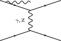
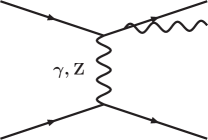
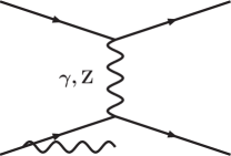
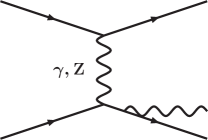
Figure 3: $t$-channel bremsstrahlung contributions to process $e^{-}e^{-}\rightarrow e^{-}e^{-}\gamma$. $u$-channel contributions are obtained by crossing.

The integration variable $v$ in Eq. (32) describes the inelasticity of the reaction, the deviation from the 2-body kinematic constraint $s+u+t=4m^{2}$. The kinematically allowed region for variable $v$ is given by chew-low

$$v\leq v^{\rm lim}=\frac{2(s+t-4m^{2})}{1+\sqrt{(1-4m^{2}/s)(1+4m^{2}/t)}}\approx s+t$$ (36)

The limit $v=v^{\rm lim}$ corresponds to the collinear singularity $u=0$. However, for E158, which only detects scattered electrons with laboratory energy $E^{\prime}\geq E_{\rm cut}\approx 11$ GeV, the integration region is further restricted to $u^{\max}=2m(m-E_{\rm cut})$ and

$$v^{\max}=s+t+u^{\max}-4m^{2}\,.$$ (37)

The squares of the matrix elements $M_{ij}^{R}$ are given by

$$M^{R}_{ij}=(M^{R}_{ij})_{zz}+(M^{R}_{ij})_{zv}+(M^{R}_{ij})_{vz}+(M^{R}_{ij})_{vv}$$ (38)

for $ij=13,31,11,33$, and

$$M^{R}_{ij}=(M^{R}_{ij})_{f}+(M^{R}_{ij})_{l}+(M^{R}_{ij})_{tu}+(M^{R}_{ij})_{s}$$ (39)

for $ij=12,14,32,34$, where the traces of the appropriate $\gamma$-matrix combinations are multiplied by the density matrices and the corresponding propagators

$${(M^{R}_{ij})}_{zz} = {\mbox{T}r}[G_{1}^{\mu\alpha}\rho^{ij}(k_{1}){G_{1}^{\nu\alpha}}^{T}\Lambda(k_{2})]{\mbox{T}r}[\gamma_{\mu}\rho^{ij}(p_{1})\gamma_{\nu}\Lambda(p_{2})]D^{it_{1}}D^{jt_{1}},$$

$${(M^{R}_{ij})}_{zv} = {\mbox{T}r}[G_{1}^{\mu\alpha}\rho^{ij}(k_{1})\gamma_{\nu}\Lambda(k_{2})]{\mbox{T}r}[\gamma_{\mu}\rho^{ij}(p_{1}){G_{2}^{\nu\alpha}}^{T}\Lambda(p_{2})]D^{it_{1}}D^{jt},$$

$${(M^{R}_{ij})}_{vz} = {\mbox{T}r}[G_{2}^{\mu\alpha}\rho^{ij}(p_{1})\gamma_{\nu}\Lambda(p_{2})]{\mbox{T}r}[\gamma_{\mu}\rho^{ij}(k_{1}){G_{1}^{\nu\alpha}}^{T}\Lambda(k_{2})]D^{it}D^{jt_{1}},$$

$${(M^{R}_{ij})}_{vv} = {\mbox{T}r}[G_{2}^{\mu\alpha}\rho^{ij}(p_{1}){G_{2}^{\nu\alpha}}^{T}\Lambda(p_{2})]{\mbox{T}r}[\gamma_{\mu}\rho^{ij}(k_{1})\gamma_{\nu}\Lambda(k_{2})]D^{it}D^{jt},$$

$${(M^{R}_{ij})}_{f} = {\mbox{T}r}[G_{1}^{\mu\alpha}\rho^{ij}(k_{1}){G_{3}^{\nu\alpha}}\Lambda(p_{2})\gamma_{\mu}\rho^{ij}(p_{1})\gamma_{\nu}\Lambda(k_{2})]D^{it_{1}}D^{ju},$$

$${(M^{R}_{ij})}_{l} = {\mbox{T}r}[G_{1}^{\mu\alpha}\rho^{ij}(k_{1})\gamma_{\nu}\Lambda(p_{2})\gamma_{\mu}\rho^{ij}(p_{1}){G_{4}^{\nu\alpha}}\Lambda(k_{2})]D^{it_{1}}D^{jz_{2}},$$

$${(M^{R}_{ij})}_{tu} = {\mbox{T}r}[\gamma_{\mu}\rho^{ij}(k_{1})G_{3}^{\nu\alpha}\Lambda(p_{2})G_{2}^{\mu\alpha}\rho^{ij}(p_{1})\gamma_{\nu}\Lambda(k_{2})]D^{it}D^{ju},$$

$${(M^{R}_{ij})}_{s} = {\mbox{T}r}[\gamma_{\mu}\rho^{ij}(k_{1})\gamma_{\nu}\Lambda(p_{2})G_{2}^{\mu\alpha}\rho^{ij}(p_{1})G_{4}^{\nu\alpha}\Lambda(k_{2})]D^{it}D^{jz_{2}},$$ (40)

where

$$\Lambda(p)=\hat{p}+m,\ \hat{p}=\gamma^{\mu}p_{\mu},$$ (41)

$$G_{1}^{\mu\alpha}=\gamma^{\mu}\frac{2k_{1}^{\alpha}-\hat{k}\gamma^{\alpha}}{-z_{1}}+\frac{2k_{2}^{\alpha}+\gamma^{\alpha}\hat{k}}{z}\gamma^{\mu},$$ (42)

$$G_{2}^{\mu\alpha}=\gamma^{\mu}\frac{2p_{1}^{\alpha}-\hat{k}\gamma^{\alpha}}{-v_{1}}+\frac{2p_{2}^{\alpha}+\gamma^{\alpha}\hat{k}}{v}\gamma^{\mu},$$ (43)

$$G_{3}^{\nu\alpha}=\frac{2k_{1}^{\alpha}-\gamma^{\alpha}\hat{k}}{-z_{1}}\gamma^{\nu}+\gamma^{\nu}\frac{2p_{2}^{\alpha}+\hat{k}\gamma^{\alpha}}{v},$$ (44)

$$G_{4}^{\nu\alpha}=\frac{2p_{1}^{\alpha}-\gamma^{\alpha}\hat{k}}{-v_{1}}\gamma^{\nu}+\gamma^{\nu}\frac{2k_{2}^{\alpha}+\hat{k}\gamma^{\alpha}}{z}.$$ (45)

Expressions for $M^{R}_{ij}$ for other values of $i$ and $j$ (e.g. $\{ij\}=22,44,24,42$, etc.) can be obtained from the symmetry of expressions in Eq. (40):

$${(M^{R}_{24})}_{zz} = \left.{(M^{R}_{13})}_{zz}\right|_{k_{2}\leftrightarrow p_{2}}=\left.{(M^{R}_{13})}_{zz}\right|_{k_{2}\leftrightarrow p_{2},k_{1}\leftrightarrow p_{1}}$$ (46)

$$= \left.{(M^{R}_{13})}_{vv}\right|_{k_{1}\leftrightarrow p_{1}}=\left.{(M^{R}_{13})}_{vv}\right|_{t\leftrightarrow u},$$

and

$${(M^{R}_{24})}_{vv} = \left.{(M^{R}_{13})}_{zz}\right|_{t\leftrightarrow u}.$$ (47)

Cases $\{ij\}=22,44$ are analyzed in a similar manner. The symmetry noted above is less apparent in the interference terms (indices $zv$ and $vz$):

$${(M^{R}_{24})}_{zv}+{(M^{R}_{42})}_{vz} = \left.\Bigl{[}{(M^{R}_{13})}_{vz}+{(M^{R}_{31})}_{zv}\Bigr{]}\right|_{t\leftrightarrow u}$$ (48)

and likewise for other parts in Eq. (32).

IV.1 Infrared Divergences in Bremsstrahlung Contributions

Next we need to address the issue of the infrared divergences in the bremsstrahlung cross section. According to the prescription of Bardin and Shumeiko covar , we find the infrared-divergent parts in the squares of the matrix elements that are proportional to the corresponding Born contributions:

$${(M^{R}_{ij})}_{zz}^{IR} = 4(\frac{m^{2}}{z^{2}}+\frac{m^{2}}{z_{1}^{2}}+\frac{t}{zz_{1}})M_{ij},$$ (49)

$${(M^{R}_{ij})}_{zv}^{IR}+{(M^{R}_{ij})}_{vz}^{IR} = 4(\frac{u}{zv_{1}}+\frac{s}{zv}+\frac{s}{z_{1}v_{1}}+\frac{u}{z_{1}v})M_{ij},$$

$${(M^{R}_{ij})}_{vv}^{IR} = 4(\frac{m^{2}}{v_{1}^{2}}+\frac{m^{2}}{v^{2}}+\frac{t}{v_{1}v})M_{ij},$$

$${(M^{R}_{ij})}_{f}^{IR} = (\frac{4m^{2}}{z_{1}^{2}}+\frac{2u}{z_{1}v}+\frac{2t}{zz_{1}}+\frac{2s}{zv})M_{ij},$$

$${(M^{R}_{ij})}_{l}^{IR} = (\frac{2s}{z_{1}v_{1}}+\frac{2t}{z_{1}z}+\frac{2u}{zv_{1}}+\frac{4m^{2}}{z^{2}})M_{ij},$$

$${(M^{R}_{ij})}_{tu}^{IR} = (\frac{2s}{z_{1}v_{1}}+\frac{2u}{z_{1}v}+\frac{2t}{vv_{1}}+\frac{4m^{2}}{v^{2}})M_{ij},$$

$${(M^{R}_{ij})}_{s}^{IR} = (\frac{4m^{2}}{v_{1}^{2}}+\frac{2u}{v_{1}z}+\frac{2t}{vv_{1}}+\frac{2s}{vz})M_{ij},$$

where

$$M_{11} = D^{\gamma t}D^{\gamma t}M_{e}^{\gamma\gamma\gamma\gamma}$$

$$M_{13} = D^{\gamma t}D^{Zt}M_{e}^{\gamma Z\gamma Z}$$

$$M_{31} = D^{\gamma t}D^{Zt}M_{e}^{Z\gamma Z\gamma}$$

$$M_{33} = D^{Zt}D^{Zt}M_{e}^{ZZZZ}$$

$$M_{12} = D^{\gamma t}D^{\gamma u}M_{o}^{\gamma\gamma\gamma\gamma}$$

$$M_{14} = D^{\gamma t}D^{Zu}M_{o}^{\gamma Z\gamma Z}$$

$$M_{32} = D^{\gamma u}D^{Zt}M_{o}^{Z\gamma Z\gamma}$$

$$M_{34} = D^{Zt}D^{Zu}M_{o}^{ZZZZ}\ .$$ (50)

The complete $R$-contribution to the cross section is infrared-divergent, but can be separated into an infrared-infinite part $\sigma_{IR}^{R}$ and the finite part $\sigma^{R}_{F}$:

$$\sigma^{R}=\sigma^{R}_{IR}+\sigma^{R}_{F}\ .$$ (51)

The IR-divergent part of the bremsstrahlung matrix elements, proportional to the Born contributions, can be constructed from Eq. (49) according to Eq. (32). The finite contribution to the cross section is then obtained by subtraction

$${(M^{R}_{ij})}^{F}={M^{R}_{ij}}-{(M^{R}_{ij})}^{IR},$$ (52)

The infrared-divergent part of Eq. (51), integrated over variables $k$ and $v$ is given in terms of a finite photon mass $\lambda$ by my3

$$\sigma_{IR}^{R}=\frac{2\alpha}{\pi}\ln\frac{(v^{\max})^{2}}{s\lambda^{2}}(\ln\frac{tu}{m^{2}s}-1)\sigma^{0}\ .$$ (53)

The integration over the phase space of the bremsstrahlung photon is performed analytically, and integration over variable $v$ is done numerically due to complexity of the integral expressions. The photon phase space integral can be written as bu-ka

$$I[A] = \frac{1}{\pi}\int\frac{d^{3}k}{k_{0}}\delta[(k_{1}+p_{1}-k_{2}-k)^{2}-m^{2}][A]=\frac{1}{\pi}\int\limits_{t_{1}^{\min}}^{t_{1}^{\max}}\ dt_{1}\int\limits_{{z}^{\min}}^{{z}^{\max}}\frac{dz}{\sqrt{R_{z}}}[A],$$ (54)

where $R_{z}$ is the Gramm determinant (modulo $-1$), and can be parameterized as a second-order polynomial in $z$ as

$$R_{z}=A_{z}z^{2}+2B_{z}z+C_{z}\ .$$ (55)

Coefficients $A_{z}$, $B_{z}$, and $C_{z}$ are given by the following expressions:

$$A_{z} = 4m^{2}t-(v-t)^{2},$$

$$B_{z} = Et_{1}+F$$

$$E = v(u-2m^{2})-st,\ F=t(2m^{2}v+st-sv),$$

$$C_{z} = -(At_{1}^{2}+2Bt_{1}+C),$$ (56)

$$A = (s-v)^{2}-4m^{2}s\ ,$$

$$B = -st(s-v-4m^{2})-2m^{2}v^{2}\ ,$$

$$C = st^{2}(s-4m^{2})\ .$$

Integration limits $z^{\min/\max}$ and $t_{1}^{\min/\max}$ are solutions of the equations $R_{z}=0$ and $z^{\min}=z^{\max}$:

$$z^{\min/\max} = \frac{-{B_{z}}\pm\sqrt{B_{z}^{2}-A_{z}C_{z}}}{A_{z}}$$ (57)

$$t_{1}^{\min/\max} = \frac{v(t-v)+2m^{2}t\mp v\sqrt{-A_{z}}}{2(v+m^{2})}$$ (58)

This set of variables makes integration more convenient.

Expressions for ${(M^{R}_{ij})}^{F}$ are computed using symbolic manipulation program REDUCE reduce but are excessively complex to be listed here. They are available as subroutines in the Fortran program rcAPV. The relevant integrals, listed in the Appendix of Ref. zyk , were computed both analytically and numerically.

V Cancellation of Infrared Singularities

Adding infrared-divergent parts of $V$- and $R$-contributions given in Eq. (31) and Eq. (53)) together with the IR-finite pieces, we obtain the finite expression for the radiatively-corrected cross section, free of non-physical parameters:

$$\sigma = \sigma^{0}+\sigma^{C}$$

$$\sigma^{C} = \sigma_{{IR}}^{V}+\sigma_{{IR}}^{R}+\sigma^{R}_{F}+\sigma^{Ver}_{F}+\sigma^{B}_{F}$$

$$= \frac{\alpha}{\pi}(4\ln\frac{v^{{max}}}{m\sqrt{s}}(\ln\frac{tu}{m^{2}s}-1)+\delta_{1}^{S}+\delta_{1}^{H})\sigma^{0}+\sigma^{Ver}_{F}+\sigma^{B}_{F}+\sigma^{R}_{F}\ ,$$

where

$$\delta_{1}^{S} = \ln\frac{s(s+t)}{m^{4}}-\frac{1}{2}l_{m}\ln\frac{s^{2}(s+t)^{2}}{-tm^{6}}-\frac{1}{2}l_{r}^{2}-2l_{r}l_{m}+l_{m}-l_{m}^{2}-\frac{\pi^{3}}{3}+1,$$

$$\delta_{1}^{H} = \int\limits_{0}^{v^{max}}dv\Bigl{(}-\frac{2}{v}\ln(1-\frac{v}{s})+\frac{2}{v}\ln(1-\frac{v}{t})+\frac{2}{v}\ln(1-\frac{v}{s+t})-\frac{1}{v}\ln(1+\frac{v}{m^{2}})$$ (60)

$$+\frac{2}{s+t-v}\ln\frac{s+t-v}{m^{2}}-\frac{1}{s-v}\ln\frac{(s-v)^{2}}{m^{2}\tau}-\frac{1}{v-t}\ln\frac{(v-t)^{2}}{m^{2}\tau}-\frac{1}{\tau}\Bigr{)},$$

$$l_{m}=\ln\frac{-t}{m^{2}},\ l_{r}=\ln\frac{s+t}{s},\ \tau\equiv v+m^{2},$$

VI Results and Discussion

VI.1 Numerical Results

In the following, we evaluate the effect of the bremsstrahlung radiative corrections on the parity-violating asymmetry $A_{LR}$ in the scattering of the longitudinally polarized electrons off unpolarized target electrons. We consider the kinematic conditions that correspond to the experimental setup of the SLAC E158 experiment E158 , i.e. beam energies of $45$ and $48$ GeV. E158 setup is such that the radiated photon is not detected. Moreover, the scattered electrons are only detected if their energy is above the threshold $E^{\prime}\geq 11$ GeV; this restriction limits the range of integration over variable $v$ as given in Eq. (37).

The relative corrections to the cross section and asymmetry can be defined as

$$\delta\sigma=\frac{\sigma-\sigma^{0}}{\sigma^{0}}\ ,\ \delta A=\frac{A_{LR}-A_{LR}^{0}}{A_{LR}^{0}},$$ (61)

where $A_{0}$ is the Born asymmetry, and $A^{RC}$ is the radiatively corrected asymmetry.

The Born cross section $\sigma^{0}$, the radiatively corrected cross sections $\sigma^{\mathrm{brem}}$ (which includes only soft and hard bremsstrahlung corrections and results of IR cancellation) and $\sigma^{QED}$ (full QED corrections), as well as the asymmetry $A_{LR}$ are shown as a function of variable $y$ in Fig. 4 for beam energy of $E=45$ GeV. Fig. 5 shows the double-differential cross section $d^{2}\sigma/dE^{\prime}/dy$ and the asymmetry $A_{LR}$ as a function of the scattered electron energy in the lab frame $E^{\prime}$ for a fixed $y=0.5$. This double-differential cross section is used to properly average the radiative corrections over the experimental acceptance. The corrections to cross section and asymmetry are shown in Fig. 6. The numerical precision of the corrections is about $0.1\%$.

We find that at fixed value of $y=0.5$ and $E=45$ GeV ($Q^{2}=0.023~{}\mathrm{GeV}^{2}$), hard bremsstrahlung reduces the value of the parity-violating asymmetry by $\approx 1\%$. Contribution from the $\gamma\gamma$ and $\gamma Z$ box diagrams is also negative and reduces the asymmetry by $\approx 5\%$, so that the total QED correction at $y=0.5$ and $E=45$ GeV is $-6.2\%$.

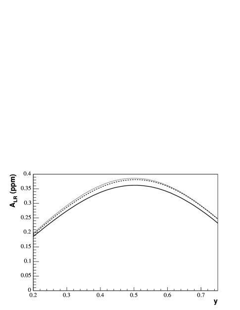
Figure 4: Differential cross section (left) and asymmetry $A_{LR}$ (right) as a function of $y$ for beam energy $E=45$ GeV. Dotted line shows the Born cross section and asymmetry, effects of bremsstrahlung corrections are displayed by dashed lines, and the solid line is the result of the full QED corrections. The plots are cut off at $y\approx 0.75$ by the E158 spectrometer acceptance ($E^{\prime}>11$ GeV).

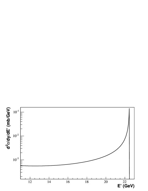
Figure 5: Møller scattering cross section (left) and asymmetry $A_{LR}$ (right) as a function of scattered electron energy $E^{{}^{\prime}}$ for beam energy $E=45$ GeV and $y=0.5$.

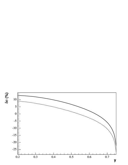
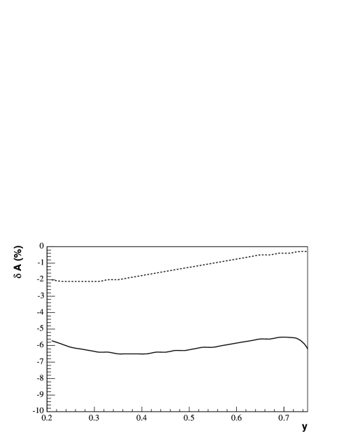
Figure 6: Relative corrections to the Møller scattering cross section (left) and to the parity-violating asymmetry $A_{LR}$ (right) as a function of $y$. Dashed line includes bremsstrahlung corrections, and the solid line is the result of the full first-order QED calculation.

At fixed scattering angles, radiative effects move events towards lower values of $y$. Therefore, even though at a fixed value of $y=0.5$ the hard bremsstrahlung correction is negative, the net change of the asymmetry, integrated over E158 acceptance $-0.5\leq\cos\Theta\leq 0$ at $E=45$ GeV is $\langle\delta A^{\mathrm{brem}}\rangle\approx+1\%$. The full QED correction, including $\gamma\gamma$ and $\gamma Z$ boxes, is $\langle\delta A^{QED}\rangle=-4.5\%$.

VI.2 Factorization of QED Radiative Corrections and NLO Uncertainties

At leading order, corrections to the parity-violating asymmetry from the diagrams involving photons (i.e. soft and hard bremsstrahlung, $\gamma\gamma$ and $\gamma Z$ boxes, and photonic vertex diagrams) are proportional to the product $v^{Z}a^{Z}$. In the OS scheme, these contributions are strictly proportional to the Born asymmetry. In other words, in the OS scheme, the relative corrections to the asymmetry due to QED diagrams are independent of the weak mixing angle, and can be factorized out. We can write

$$A_{LR}^{QED}=\mathcal{A}^{0}(Q^{2},y)(1+\delta A^{QED})\left(1-4\sin^{2}\theta_{W}\right)\,$$ (62)

where $\mathcal{A}^{0}(Q^{2},y)$ is the Born analyzing power defined in Eq. (17) and $\delta A^{QED}$ is the relative radiative correction. For $E=45$ GeV and $y=0.5$, full QED correction is $\delta A^{QED}=-0.061$, and the average over E158 kinematics (beam energies of 45 and 48 GeV and $-0.5\leq\cos\Theta\leq 0$) is $\langle\delta A^{QED}\rangle_{\mathrm{E158}}=-0.043$.

Virtual corrections, such as vacuum polarization and box and vertex diagrams with heavy gauge bosons, are not in general proportional to $v^{Z}a^{Z}$, and spoil the simple factorization of Eq. (62). Nevertheless, one can relate the leading-order asymmetry to the Born-level formula through the set of multiplicative and additive corrections:

$$A_{LR}(Q^{2},y)=\mathcal{A}^{0}(Q^{2},y)\rho(Q^{2})(1+\delta A(Q^{2},y))\left(1-4\sin^{2}\theta_{W}^{\rm eff}(Q^{2})+\Delta(Q^{2})\right)\,.$$ (63)

Here the effective mixing angle relevant for a scattering process at momentum transfer $Q$ is defined through the form-factor $\kappa(Q^{2})$ (in OS scheme) or $\hat{\kappa}(Q^{2},\mu^{2})$ (in $\overline{\mbox{MS}}$ scheme):

$$\sin^{2}\theta_{W}^{\rm eff}(Q^{2})\equiv\kappa(Q^{2})\sin^{2}\theta_{W}^{OS}=\hat{\kappa}(Q^{2},\mu^{2})\sin^{2}\hat{\theta}_{W}(\mu^{2})\ .$$ (64)

In $\overline{\mbox{MS}}$ scheme, one typically chooses $\mu=m_{Z}$.

All corrections in Eq. (63) are of order $\mathcal{O}(\alpha)$ but have a different physical meaning. The form-factor $\kappa=1+\mathcal{O}(\alpha)$ defines the momentum dependence (running) of the effective weak mixing angle. We would like to define it in a process-independent way, such that various experimental measurements could be directly compared in terms of $\sin^{2}\theta_{W}^{\rm eff}$. Typically, $\kappa$ includes contributions from $\gamma-Z$ mixing and anapole moment diagrams (Fig. 2a-c) cz-marc , but may include other terms sirlin ; erler-musolf . In definition of Ref. cz-marc , carried out in $\overline{\mbox{MS}}$ scheme with $\sin^{2}\hat{\theta}_{W}(m_{Z}^{2})\equiv\hat{s}^{2}=0.23120\pm 0.00015$ ref:PDG2004 , $\hat{\kappa}(Q^{2}=0,\mu^{2}=m_{Z}^{2})=1.0298\pm 0.0026$

The form-factor $\rho(Q^{2})=1+\mathcal{O}(\alpha)$ is a low-energy ratio of the neutral weak coupling to the charge coupling. It depends on the choice of the Fermi constant $G_{F}$ in Eq. (17); for $G_{F}$ derived from the muon-decay constant $G_{\mu}$, this correction is cz-marc $\rho=1.0012\pm 0.0005$. $\rho$ contains logarithmic dependence on the Higgs mass (we use $m_{H}=113_{-40}^{+56}$ GeV ref:PDG2004 ) and linear dependence on the top quark mass ($m_{t}=177\pm 4$ GeV ref:PDG2004 ).

The remaining first-order corrections are included in Eq. (63) as factors $\delta A(Q^{2},y)$ and $\Delta(Q^{2})$. $\Delta(Q^{2})$ typically includes box diagrams with two heavy bosons, and $\delta A(Q^{2},y)$ contains the kinematics-dependent factorizable QED corrections computed in Section VI.

The only remaining question is evaluating the next-to-leading order correction uncertainties. Normally, NLO corrections would be of order $\mathcal{O}(\alpha)$ of the LO terms. However, we have to pay special attention to the logarithmically-enhanced contributions in the $\gamma Z$ box diagrams, e.g. terms proportional to $\ln(m_{Z}^{2}/s)$ in Eq. (29).

The effective $Z^{0}$-electron coupling, $Q_{w}=-\rho(1-4\sin^{2}\theta_{W})$ changes by about $40\%$ between zero momentum transfer and $Z^{0}$ pole cz-marc . Since the box diagrams in Fig. 2 involve integration over internal momenta of the photon and $Z^{0}$ propagators, a complete calculation of the box diagrams has to take into account the momentum dependence of $Q_{w}$ and $\alpha$. Strictly speaking, the momentum dependence of the weak or electromagnetic charges in the box integrals is a next-to-leading order effect, and is beyond the scope of this work. However, a judicious choice of the coupling at leading order could reduce the NLO corrections.

Czarnecki and Marciano cz-marc have argued that the NLO errors are reduced if the $\gamma Z$ box diagrams are evaluated in $\overline{\mbox{MS}}$ scheme with the average value of the weak mixing angle

$$\langle\sin^{2}\theta_{W}\rangle\equiv\frac{\sin^{2}\theta_{W}(0)+\sin^{2}\theta_{W}(m_{Z}^{2})}{2}$$ (65)

since the relevant integrals over the internal momentum $k$ are dominated by the poles near $k^{2}\sim 0$ and $k^{2}\sim m_{Z}^{2}$. Similar arguments apply to the value of the fine structure constant in the $\gamma Z$ box diagrams. Thus, following the spirit of this argument, we move the leading logarithmic contribution to the $\gamma Z$ box diagrams cz-marc

$$\Delta_{\gamma Z}(Q^{2})=-\frac{22}{3}\frac{\alpha(Q^{2})}{4\pi}\left(1-4\sin^{2}\theta_{W}(Q^{2})\right)\ln\frac{m_{Z}^{2}}{s}$$ (66)

from the multiplicative correction $\delta A(Q^{2},y)$ to the additive correction $\Delta(Q^{2})$. Moreover, we use the average value $\langle\Delta_{\gamma Z}\rangle\equiv(\Delta_{\gamma Z}(0)+\Delta_{\gamma Z}(m_{Z}))/2$ in the expression for $\Delta(Q^{2})$, and treat the spread $|\Delta_{\gamma Z}(0)-\Delta_{\gamma Z}(m_{Z})|/2$ as an estimate of the NLO uncertainties. This choice keeps all of the experimental acceptance dependence in the multiplicative correction $1+\delta A(Q^{2},y)$, properly propagates the bremsstrahlung corrections, and reduces the overall size of the theoretical uncertainties. For experimental kinematics of the E158 experiment, we find

$$\delta A(Q^{2},y)=0.006\pm 0.005\ ,$$ (67)

where the uncertainty is dominated by the possible variations of the experimental acceptance and numerical precision. Employing the calculation of Ref. cz-marc for the terms $\hat{\kappa}$ and $\rho$, the corresponding contributions from the $WW$ and $ZZ$ box diagrams, and our definition of $\langle\Delta_{\gamma Z}\rangle$ term, the residual additive correction in Eq. (63) is

$$\Delta(Q^{2}) = \langle\Delta_{\gamma Z}\rangle+\frac{\alpha(m_{Z}^{2})}{4\pi\hat{s}^{2}}-\frac{3\alpha(m_{Z}^{2})}{32\pi\hat{s}^{2}(1-\hat{s}^{2})}(1-4\hat{s}^{2})\left[1+(1-4\hat{s}^{2})\right]=-0.0007\pm 0.0009$$ (68)

where the uncertainty is dominated by our conservative estimate of the NLO terms.

The fact that both corrections $\delta A(Q^{2},y)$ and $\Delta(Q^{2})$ are small is somewhat accidental. $\delta A(Q^{2},y)$ is dominated by the bremsstrahlung contributions and the infrared parts of the $\gamma\gamma$ and $\gamma Z$ diagrams that happen to cancel each other for the asymmetric acceptance of the E158 spectrometer. On the other hand, $\Delta(Q^{2})$ is small at the $Q^{2}$ of E158 due to the cancellation between the $WW$ box diagrams and the large logarithmic contribution in the $\gamma Z$ box. Such precise cancellation is not expected at lower momentum transfers, or for other processes, such as elastic $ep$ scattering. For example, at $y=0.5$ and $E=12$ GeV, which corresponds to the idealized kinematics for a proposed Møller scattering experiments at the Jefferson Lab JLab12 , the corrections would be

$$\delta A(Q^{2},y=0.5)_{12~{}\mathrm{GeV}}=-0.024\pm 0.005\ ,\Delta(Q^{2})_{12~{}\mathrm{GeV}}=-0.0011\pm 0.0010\ .$$ (69)

For a 250 GeV fixed target Møller experiment, e.g. at a future Linear Collider MollerLC , one would find

$$\delta A(Q^{2},y=0.5)_{250~{}\mathrm{GeV}}=-0.012\pm 0.005\ ,\Delta(Q^{2})_{12~{}\mathrm{GeV}}=-0.0002\pm 0.0007\ .$$ (70)

VII Conclusions

In conclusion, we have computed the QED corrections to the parity-violating left-right asymmetry $A_{LR}$ in Møller scattering. We used a covariant method for removing infrared divergences without introducing unphysical cutoffs. For the kinematics of SLAC E158 experiment, the overall corrections appear to be small, due to a fortuitous cancellation between electroweak and electromagnetic terms. We reduce the theoretical uncertainties due to higher order logarithmic terms by the appropriate choice of the couplings used to compute the box diagram contributions. Our calculation is applicable to a wide range of fixed target energies, from the proposed Møller scattering experiments at 12 GeV at the Jefferson Lab JLab12 , to the possible fixed target experiments at a future Linear Collider MollerLC .

VIII Acknowledgments

The authors would like to thank Peter Bosted, Stanley Brodsky, Lance Dixon, Krishna Kumar, William Marciano, Michael Peskin, and Frank Petriello for stimulating discussions. VZ and JS would like to thank SLAC staff for the generous hospitality during their visits. This work has been partially supported by the National Science Foundation under grant PHY-0140366.

References

• (1) Ya.B. Zel’dovich, Sov. Phys. JETP 94, 262 (1959).
• (2) Particle Data Group, S. Eidelman et al., Phys. Lett. B592, 2004 (1).
• (3) W.J. Marciano and J.L. Rosner, Phys. Rev. Lett. 65, 2963 (1990).
• (4) SLAC E158 Collaboration, P.L. Anthony et al., Phys. Rev. Lett. 92, 181602 (2004); preprint hep-ex/0504049.
• (5) A. Czarnecki and W.J. Marciano, Phys. Rev. D53, 1066 (1996).
• (6) A. Denner and S. Pozzorini, Eur. Phys. J. C7, 185 (1999).
• (7) V. Zykunov, Yad. Fiz. 67, 1366 (2004).
• (8) J. Arrington et al., Nucl. Instrum. Methods A311, 39 (1992); H.R. Band et al., Nucl. Instrum. Methods A400, 24 (1997).
• (9) N.M. Shumeiko and J.G. Suarez, J. Phys. G. 26, 113 (2000).
• (10) A. Ilyichev and V. Zykunov, preprint hep-ph/0504191.
• (11) D.Yu. Bardin and N.M. Shumeiko, Nucl. Phys. B127, 242 (1977); Sov. J. Nucl. Phys. 29, 969 (1979).
• (12) C. Møller, Ann. Phys. 14, 532 (1932).
• (13) LEP Electroweak Working Group, SLD Electroweak and Heavy Flavor Working groups, preprint hep-ex/0312023.
• (14) C.A. Heush, Int. J. Mod. Phys. A15, 2347 (2000).
• (15) F.J. Petriello, preprint SLAC-PUB-9532, hep-ph/0210259 (2002).
• (16) M. Böhm et al., Forschr. Phys. 34, 687 (1986).
• (17) W. Hollik, Forschr. Phys. 38, 165 (1990).
• (18) M. Böhm and H. Spiesberger, Nucl. Phys. B294, 1081 (1987).
• (19) G.F. Chew and F.E. Low, Phys. Rev. 113, 1640 (1959).
• (20) N.M. Shumeiko, S.I. Timoshin, and V.A. Zykunov, J. Phys. G23, 1593 (1997).
• (21) E. Byckling and K. Kajantie, Particle Kinematics, John Wiley & Sons (1973).
• (22) A.C. Hearn, REDUCE User’s Manual for Version 3.4.1, Santa Monica, CA 90407-2138 (1992)
• (23) P. Anthony et al., Phys. Rev. Lett. 92, 2004 (181602).
• (24) A. Ferroglia, G. Ossola, and A. Sirlin, Eur. Phys. J. C34, 2004 (165).
• (25) J. Erler and M.J. Ramsey-Musolf, preprint hep-ph/0409169.
• (26) J. Arrington et al., Conceptual Design Report for the Science and Experimental Equipment for the 12 GeV Upgrade of CEBAF (2005).
• (27) L. Keller et al., preprint SLAC-PUB-8725, physics/0101070 (2001).